Automated Segmentation and Classification of Aerial Forest Imagery

Abstract

Monitoring the health and safety of forests has become a rising problem with the advent of global wildfires, rampant logging, and reforestation efforts. This paper proposes a model for the automatic segmentation and classification of aerial forest imagery. The model is based on U-net architecture and relies on dice coefficients, binary cross-entropy, and accuracy as loss functions. While models without autoencoder-based structures can only reach a dice coefficient of 45%, the proposed model can achieve a dice coefficient of 79.85%. In addition, for barren adn dense forestry image classification, the proposed model can achieve 82.51%. This paper demonstrates how complex convolutional neural networks can be applied to aerial forest images to help preserve and save the forest environment.

1. Introduction

With the looming threat of climate change growing increasingly fraught in recent times, weather events such as heat waves and gradual temperature increases have become more prominent. These effects are especially apparent in dry parts of the world such as California, which has lately become a hot spot for wildfires of enormous magnitude. Wildfires in the 21st century have not only critically endangered forests but have also polluted the air, displacing thousands of people and even taking human lives [1]. When managing forests, appropriate precautions should be taken against forest fires as they take a heavy toll on lives and the surroundings. To avert or mitigate the damage produced, researchers often use the help of aerial images [2]. This technology has substantial potential value and will be explored throughout this paper.

In the modern world, another issue arises with the logging industry, which has become a common practice amidst the increasing demand for wood. The simplest way to match this new demand is to simply cut down as many trees as needed. As a result, this irrevocably disrupts fragile forest ecosystems and increases pollution, similarly to the effects of the wildfires described above.

However, cutting down trees also has a counterpart—reforestation. In order to combat the decline of rainforests and other naturally formed woodlands, various entities have begun to plant self-sustaining forests. This can be seen as a method of combating the destructive effects of logging and wildfires. At the end of the day, the forests on Earth provide shelter for a wide array of animals and take CO${}_2$ out of the atmosphere, using the process of photosynthesis in order to convert it to precious oxygen.

This presents the issue of keeping track of forest health and safety in order to minimize human casualty and incidents as well as collateral damage to our environment. With the frequent fluctuation of forest sizes, a method to easily track and monitor the border sizes of forests is crucial in this era. Now, with the help of new innovations in computer vision and convolutional neural networks, it is possible to take commonly found satellite images of forest borders or areas and delineate the bounds of the forests. The process for creating masks for images has not yet been perfected; however, it has improved a lot. Despite the rapid development of computer vision algorithms for detecting objects in an image, the task of the segmentation of images for remote sensing applications with respect to the Earth’s surface has not been automated to the same extent as the accuracies observed in manual marking [3]. If this process is expanded over a few years with satellite images taken from the same locations, previous AI-generated masks can be compared and the effect on the size of forests is easily evident [3].

1.1. Literature Review

A deep network U-net [3] produced a deep learning algorithm capable of segmenting forests in high-resolution satellite images. However, the dataset was limited to 17 images in total with an imbalanced training set, and despite image augmentations to try to increase the size, it did not show high results in detection. Ref. [4] performed segmentation with a CNN to segment satellite images into different classifications but suffered from isolated satellite and segmentation photos made at different times leading to inaccuracy. Another segmentation method using a CNN [1] identified forest fires by using aerial images, achieving high fire-detection accuracy with a novel image classification method. Ref. [5] also created a conceptually easy model for the literature, which efficiently segments different types of tissues in breast biopsy images while simultaneously predicting a discriminative map for identifying important areas in an image. Their model, Y-net, improved the diagnostic classification accuracy by 7% over state-of-the-art methods for diagnostic classification [5].

Ref. [6] created a high-resolution dataset of forest aerial imagery for classification and feature identification with deep learning models. Ref. [7] performed segmentation by using a CNN to cluster trees as superpixels and with color-threshold-implemented pixel-based segmentations. Ref. [8] introduced a method to effectively separate forest and dense grass in normalized difference vegetation index (NDVI) images used to analyze satellite photography. Using only spectral information to distinguish forests from grass areas, the proposed method is proved to be an effective way to separate these features but also noted that deploying machine learning algorithms would lead to greater accuracies for complex features.

Although these previous methods provide some solutions to the problem of monitoring forest size, health, and safety, none of them fully address the issue. With forest fires on the rise, climate change destroying these critical ecosystems, and logging devastating the habitats of endangered species and large swathes of forests, it becomes all the more crucial that we accurately monitor the situation of our forests. The key to solving this problem lies in aerial photography, and the novel method proposed in this paper provides an accurate solution for distinguishing forests in aerial imagery. While other papers and studies attempted to address this issue in the past, our paper provides a highly accurate CNN model with a comprehensive dataset and precision in forest detection.

1.2. Major Contributions

The major contribution of this paper is presented below:

1.

This model contributes many advantages because it provides two different results: a mask and a classification. Our segmentation provides a black and white image that is an overlay of the inputted image that determines which parts are forest and which are not. Moreover, our classification output determines whether the input image is more than half the forest or not. By inputting a satellite image into our model, these results can be output simultaneously.

2.

Another crucial aspect to our model is comprehensiveness and explainablity. At its simplest level, the model is taking a satellite image and highlighting the parts that look similar to a forest white, and everything other than a forest is highlighted with black. That is essentially what our model does, taking an image and applying various filters on it to end up with a black and white image depicting which parts contain forests and which do not.

3.

In addition to providing useful results and unlike previous CNN models identifying aerial forest imagery, our model also competes with high accuracies as our classification model has an 82.51 percent accuracy in determining whether the image is 50 percent or more forest. Our mask-generating (segmentation) model additionally has a 79.85 percent accuracy in correctly determining whether each part of the image is a forest or not. This paper presents a novel CNN model with high accuracies that can be used for forest segmentation and can effectively distinguish forest areas.

2. Proposed Model

The motivation of the proposed model is to create masks highlighting regions of dense forests for the Forest Aerial Image dataset as well as to classify the images into two categories: dense and barren. Dense means that the image comprises more than 50 percent of forests, and barren means the image comprises forests at 50 percent or less. The model can take any satellite images with certain portions in the image being forest areas. The model is able to produce two outputs: a generated mask pinpointing the area of the forest and a label showing whether the image is barren or dense.

2.1. Convolutional Operation

It is important to first talk about a concept called the convolutional operation. The convolutional operation plays a huge role in all Convolutional Neural Networks (CNN). The convolutional operation is used to estimate the weighted sum of a pixel of an image along with its neighboring pixels. This weighted sum is calculated by adding the products of individual pixels and their weights using a 2D matrix called a kernel. The kernel’s matrix is composed of weights that will glide over an image by applying the convolutional operation as it proceeds. For any given image, a kernel will start at the top-left part of the image. This sum will represent the chunk that the kernel is currently covering. The kernel moves horizontally by a stride or the number of tiles it shifts, and the operation is then applied to the next set of pixels. If a filter does not fit the input image, zero-padding is used, which sets any values outside the image to zero.

2.2. Convolutional Neural Networks

Consisting of convolutional layers, pooling layers, and a fully-connected layer, CNNs highlight important patterns in images that the model can identify to provide more consistent and accurate predictions. Most basic CNNs are composed of convolutional layers, pooling layers, and a fully connected layer [9]. The convolutional operation plays a major role in CNNs, as it is the backbone for the convolutional layer. Convolutional layers are where most of the work is performed, and they use the convolutional operation to create a map of all the outputs from the different kernels stacked on top of each other. After each convolutional operation, the network applies a rectified linear unit (ReLu). Pooling layers are used after convolutional layers. Pooling layers also use a kernel that slides over the image, but instead of applying a formula, it downsamples the image by simplifying the information in the image. There are two types of pooling layers: max pooling and average pooling. Max pooling chooses the largest number that the kernel is covering. This is the more commonly used type of pooling because it preserves distinct features. In the fully connected layer, nodes from the output layer directly, or linearly, connect to nodes in previous layers.

2.3. U-Net

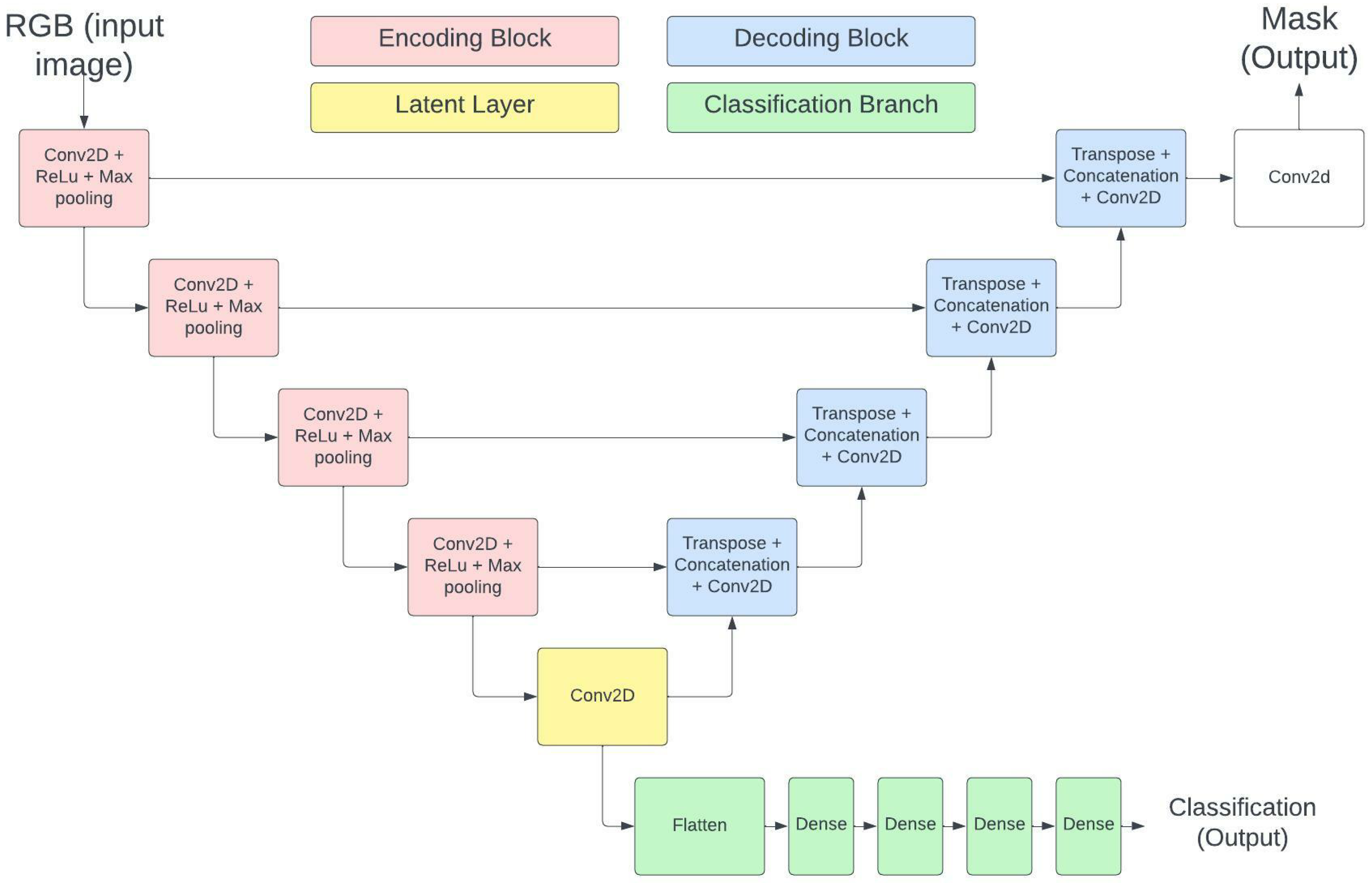
The model we used is a type of Convolutional Neural Network called U-net, which is excellent for distinguishing borders, allowing us to form masks for the Forest Aerial Image dataset well [10]. U-nets are based on an autoencoder structure [11]. Autoencoders follow an encode–decode structure that shrinks and expands the input, respectively. However, these basic autoencoders did not specialize in image segmentation. U-nets utilize the convolutional operation, allowing images to be processed with the autoencoder structure. More specifically, the first half of a U-net, called the contracting path, utilizes the convolutional operation to downsample the image. The contracting path consists of an encoding process that is repeated several times. This process consists of two convolutional layers with a 2 × 2 kernel, ReLu activation, and a max pooling layer. An image put through this process will result in a shrinkage in the image’s width and height but the image’s depth will increase. After the contracting path, a latent layer consisting of two additional convolutional layers with no max pooling is applied to the input. The second half of the U-net, called the expansive path, is symmetric to the contracting path, forming the u-shape the network is named after. The expansive path repeats a decoding process to expand the image back to its original dimensions. This formula is made up with a transposed-convolutional layer, a concatenation layer, and two more convolutional layers. The transposed-convolutional layer up-samples the image, returning the input to its original dimension. The concatenation process combines the current image with its corresponding image from the contracting path to combine the information from both images to obtain a more accurate prediction. Two convolutional layers without max pooling follow transposed convolution and concatenation processes. The decoding process is repeated the same number of times as the encoding process from the contracting path. At the very end of the U-net, a single convolutional layer using a 1 × 1 kernel is applied.

2.4. Multi-Output Classifier and Mask Generator

The standard U-net’s main output is a mask for the input image, meaning that any U-net will achieve half of the model’s purpose. However, in order to obtain a classification estimation as a secondary output from the model, it had to be slightly modified (see Figure 1). The classification branch begins after the latent layer but before the expansive path. The model uses the output image from the latent layer for image segmentation. In addition, the classification branch is created using three dense layers that are fully connected. The resulting image is then analyzed to determine if the image is dense (more than 50 percent forest) or barren (50 percent or less forest).

3. Application

The section starts with introducing the data. From the Introduction section, the motivation should already been discussed. Hence, the focus in this section is show readers how the data are designed in a manner that answers the research question.

3.1. Experiment Design

This application used a large satellite image dataset [10]. The dataset has two portions. First, the dataset has raw satellite images taken of woodlands. Next, the dataset contains a set of masks that correspond to a satellite image. Each mask is hand-drawn in order to represent the border of forests shown within the satellite photo.

The dataset contains 5108 unique satellite images and an additional 5108 unique masks (each of which align with a certain satellite image) [10]. Additionally, each satellite image is size 256 by 256 by 3, where dimension 3 corresponds to the individual RGB (red, green, and blue) layers of the image. Each mask’s image size is 256 by 256 by 1, with 1 corresponding to the black and white nature of the image (i.e., if a pixel is on (white) or off (black)). For image classification, we defined the classes according to the area of forestry contained in the images. This allows us to address the barren or dense level of the forestry area in the image data. Different threshold can be chosen to separate an image into two classes: dense or barren. To ensure balanced classes, the threshold is chosen such that each class contains 50% of the dataset.

In the proposed model, the data images are resized in order to gain more accuracy in the model. Originally, each image was 256 by 256 (the dimension for the number of color pixels), but after resizing the images, the size was changed to 128 by 128 (the dimension for the amount of color pixels). This helped increase the accuracy of the model in the results (Section 3.2).

It is also important to understand the loss function for both the segmentation and classification parts of our model. Segmentation uses the Sorensen–Dice Coefficient [12,13], which can be modified to be a loss function. Given two sets X and Y, masks and images, the Sorensen–Dice Coefficient is defined using Equation (1).

$$\mathcal{D}=\frac{2|X\cap Y|}{\left|X\right|+\left|Y\right|}$$

(1)

The proposed classifier branch uses binary cross-entropy as the main loss function. The binary cross-entropy, or BCE, loss function is defined in Equation (2). As one of the most popular loss function in the literature, the BCE compares the distance between the ground truth of y and prediction $\widehat{y}$. Prediction $\widehat{y}$ is produced from the last layer of the classification branch of the proposed model, which uses softmax as an activation function, to ensure the prediction is in the appropriate probability distribution [14]. The BCE has many more updated versions, which are introduced in this paper [15]. For a simple two-class classification in our paper, we use the BCE directly. The formula of BCE is formally defined in Equation (2).

$$\mathcal{L}(y,\widehat{y})=-\frac{1}{n}\sum _i^n(y_{i}log{\widehat{y}}_i+(1-y_i)log(1-{\widehat{y}}_i))$$

(2)

Classification also uses accuracy as an additional loss function, which can be defined using the confusion matrix. The confusion matrix is a performance measurement consisting of four different values: true positive (TP), false positive (FP), false negative (FN), and true negative (TN) (see Figure 2). “True” means that the network predicted correctly, so TP means that the network predicted true and it was true. “False” means that the network predicted wrong, so FP means that the network predicted the positive but it was false. Accuracy is defined using Equation (3).

$$\mathrm{Accuracy}=\frac{\mathrm{TP}+\mathrm{TN}}{\mathrm{TP}+\mathrm{FN}+\mathrm{FP}+\mathrm{TN}}$$

(3)

3.2. Results

The results of the classification are presented in

Table 1. Classification Results. This table covers the results of a simple CNN consisting of convolutional and dense layers trained only to classify the images.

Model Index	Conv Layers			Dense Layers		-
	Conv1	Conv2	Conv3	Dense1	Dense2	Kernel Size	Classification Accuracy (%)
Model 1	32	64	128	128	512	2 × 2	96
Model 2	128	64	N/A	256	512	1 × 1	92
Model 3	32	64	128	128	512	1 × 1	95

. Table 1 shows three different CNN models, each created using multiple convolutional layers with max pooling as well as a flattened layer and multiple dense layers. The number of dense layers is a tuning parameter. Model 1 consists of three convolutional layers, with 32 filters in the first layer, 64 filters in the second layer, and 128 filters in the third layer. For the dense layers, 128 neurons are used in the first layer and 512 neurons are used in the second. A kernel size of 2 by 2 was used. This model achieved the strongest accuracy of 96% out of the three models listed. Model 2 only uses 2 convolutional layers, with 128 and 64 filters respectively. This model used 256 neurons for the first dense layer and 512 neurons for the second dense layer, and used a kernel size of 1 by 1. It achieved an accuracy of 92%. Model 3 is the same as Model 1 in terms of convolutional layers and dense layers but uses a kernel size of 1 by 1, achieving an accuracy of 95%.

The results for the segmentation results are shown in

Table 2. Segmentation Results. This table covers the results from U-net models purposed to create masks. The third entry comes from another model also using forest aerial Images [3].

Model Index	Encode	Latent	Decode	Optimizer	Epochs	Dice Coef.
Model 4	{32, 64, 128, 256, 512}	1024	{512, 256, 128, 64, 32}	Adam (w. lr scheduler)	100	76.13%
Model 5	{32, 64, 128}	256	{128, 64, 32}	Adam (w. lr scheduler)	100	68.45%
Model 6	N/A	N/A	N/A	Adam	100	45%

. The results were taken from three separate U-nets consisting of only the encoding and decoding passages. Model 4 consists of five encoding operations, each with two convolutional layers and max pooling. The first convolutional layer receives 32 filters, the second receives 64 filters, the third receives 128 filters, the fourth receives 256 filters, and the fifth receives 512 filters. The latent layer receives 1024 filters. The decoding process, consisting of a transposed convolutional layer, concatenation, and two more convolutional layers, repeats five times to mirror the encoding layers. The first layer receives 512 filters, the second layer receives 256 filters, the third layer receives 128 filters, the fourth receives 64 filters, and the fifth receives 32 filters. The optimizer was Adam with a learning rate scheduler. After 100 epochs, the highest dice coefficient the model reached was 76.13%. Model 5 is similar to Model 4, except there are less layers involved. Three encoding operations were used, with the first layer receiving 32 filters, the second receiving 64 filters, and the third receiving 128 filters. The latent layer receives 256 filters. The decoding operation repeats three times, with the first layer receiving 128 filters, the second receiving 64 filters, and the third receiving 32 filters. Adam and a learning rate scheduler was used for the optimizer. After 100 epochs, the highest dice coefficient the model reached was 68.45%. Model 6 was a model created by Vladimir Khryashchev, Anna Ostrovskaya, Vladimir Pavlov, and Roman Larionov in their paper, “Forest Areas Segmentation on Aerial Images by Deep Learning” [3]. Although the number of filters was not specified, their model still followed the standard encode–decode architecture with an additional encoding passage to accommodate their model’s purpose. Their model reached a dice coefficient of 45% after 100 epochs.

In

Table 3. Classifier and Mask Generator U-net Results. This table covers the results from the model presented in this paper. It is important to note that our model outputs accuracies for both the Dice coefficient (mask accuracy) and classification.

Encode	Latent	Dense	Decode	Optimizer	Epochs	Dice Coef.	Classification Accuracy
{32, 64, 128}	256	{128, 64, 32, 2}	{128, 64, 32}	Adam (w. lr scheduler)	100	79.85%	82.51%

, the results for both the classification and segmentation for the proposed model are listed. This model is a U-net with encoding and decoding operations modified with additional dense layers branching from the latent layer, as explained in Section 2.4. The encoding operation is repeated three times, with the first layer using 32 filters, the second using 64 filters, and the third using 128 filters. The latent layer uses 256 filters. Four dense layers begin from the latent layer, with the first dense layer using 128 neurons, the second dense layer using 64 neurons, the third dense layer using 32 neurons, and the fourth dense layer using 2 neurons. The two neurons represent the two classes: dense and barren. The decoding process, branching from the latent layer, begins with 128 filters in the first layer, 64 filters in the second layer, and 32 filters in the third layer. The optimizer is Adam with a learning rate scheduler. After 100 epochs, the model reached a dice coefficient of 79.85%, and a classification accuracy of 82.51%. Our model combines the functions of segmentation and classification into one while maintaining high performance.

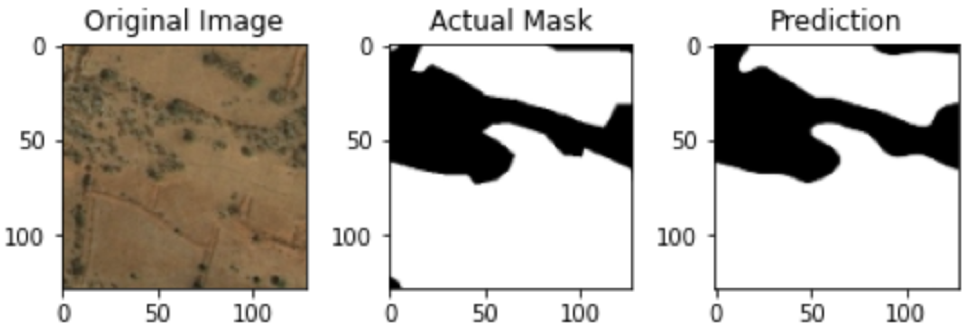
In Figure 3 below, it displays the mask prediction for a barren image from the proposed U-net model. Three images are displayed: The first two images are the original image and the mask given from the image dataset. The third image is the prediction given by the model.

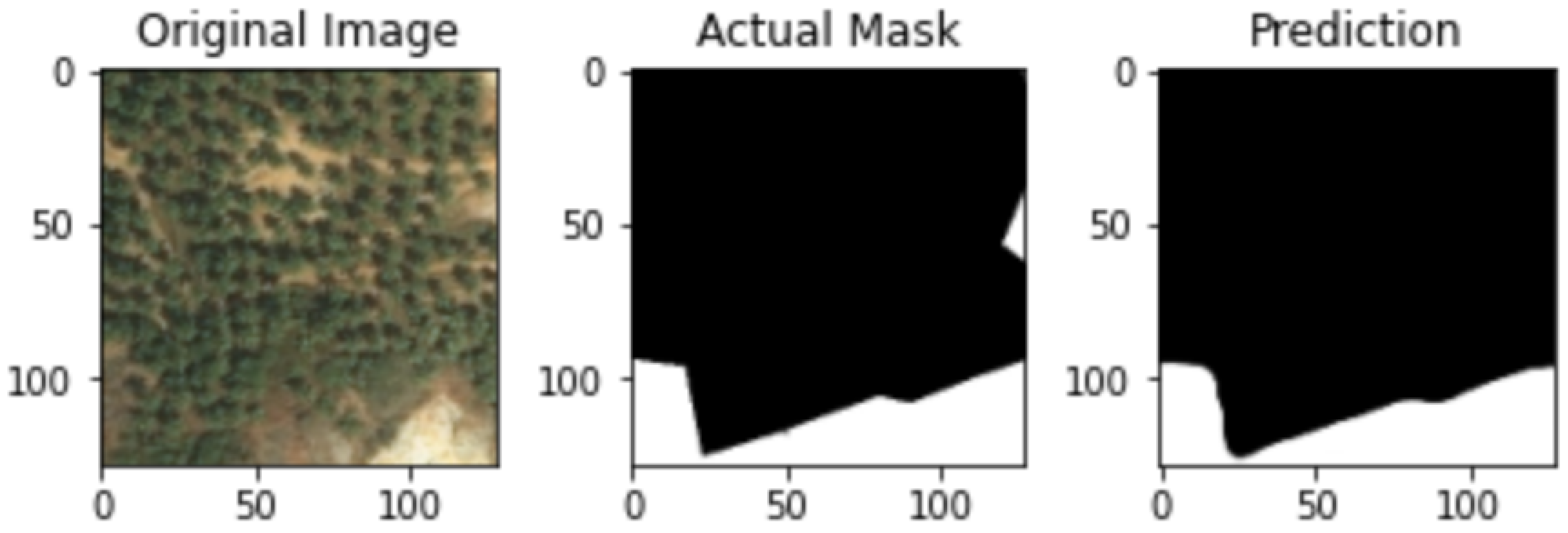
In Figure 4 below, it displays the mask prediction for a dense image from the proposed U-net model. The first two images are the original image and mask from the image dataset and the third image is the prediction given by the model.

4. Discussion and Future Scope

This study looked into the use and application of a novel CNN model to analyze aerial forest imagery in order to distinguish border sizes. Unfortunately, thus far, not a lot of research has been performed on the subject of using AI models to analyze satellite images, and the studies that have been performed suffered from small or limited datasets and insufficient accuracy. Compared to previous studies such as [3], this model provides greater accuracy, reaching a dice coefficient of 79.85% and a classification accuracy of 82.51%. To address the difficulties that previous models [4] have had with datasets, we trained our model on a more comprehensive dataset, as described in Section 3.1. Further research would entail continuing to improve the accuracy of the model as well as providing a larger and more detailed dataset. The classification of terrain into further distinctions would also provide more information and increase the accuracy of tracking borders. The application of this or future models could prove as important tools in tracking wildfires, logging, and reforestation progress.

5. Conclusions

In this study, we provided a solution to the problem of forest border tracking using a novel CNN model with high accuracy in both the segmentation and classification of aerial forest imagery. Via a U-net deep learning model, we combined both the functions of segmentation and classification while maintaining a high accuracy (82.51%) and a dice coefficient of 79.85%. This study provides a benchmark for future case studies and improves upon past ones, opening an avenue for future research in this topic. Our method and model present a innovative solution for monitoring the health of our forests and any threats to our forests.

References

- Guan, Z.; Miao, X.; Mu, Y.; Sun, Q.; Ye, Q.; Gao, D. Forest Fire Segmentation from Aerial Imagery Data Using an Improved Instance Segmentation Model. Remote Sens. 2022, 14, 3159. [Google Scholar] [CrossRef]
- Bhattacharjee, G.; Pujari, S. Aerial Image Segmentation: A Survey. Int. J. Appl. Inf. Syst. 2017, 12, 28–34. [Google Scholar] [CrossRef]
- Khryashchev, V.; Pavlov, V.; Ostrovskaya, A.; Larionov, R. Forest Areas Segmentation on Aerial Images by Deep Learning. In Proceedings of the 2019 IEEE East-West Design & Test Symposium (EWDTS), Batumi, Georgia, 13–16 September 2019; pp. 1–5. [Google Scholar]
- Guérin, E.; Oechslin, K.; Wolf, C.; Martinez, B. Satellite Image Semantic Segmentation. arXiv 2021, arXiv:2110.05812. [Google Scholar]
- Mehta, S.; Mercan, E.; Bartlett, J.; Weaver, D.; Elmore, J.G.; Shapiro, L. Y-Net: Joint segmentation and classification for diagnosis of breast biopsy images. In Proceedings of the International Conference on Medical Image Computing and Computer-Assisted Intervention, Granada, Spain, 16–20 September 2018; pp. 893–901. [Google Scholar]
- Umar, M.; Saheer, L.B.; Zarrin, J. Forest Terrain Identification using Semantic Segmentation on UAV Images. In Proceedings of the ICML 2021 Workshop on Tackling Climate Change with Machine Learning, Online, 23–24 July 2021. [Google Scholar]
- Fikri, M.Y.; Azzarkhiyah, K.; Firdaus, M.J.A.; Winarto, T.A.; Syai’in, M.; Adhitya, R.Y.; Endrasmono, J.; Rahmat, M.B.; Setiyoko, A.S.; Fathulloh; et al. Clustering green openspace using UAV (Unmanned Aerial Vehicle) with CNN (Convolutional Neural Network). In Proceedings of the 2019 International Symposium on Electronics and Smart Devices (ISESD), Badung, Indonesia, 8–9 October 2019; pp. 1–5. [Google Scholar] [CrossRef]
- Sai, S.V.; Mikhailov, E.V. Texture-based forest segmentation in satellite images. J. Phys. Conf. Ser. 2017, 803, 012133. [Google Scholar] [CrossRef]
- Long, J.; Shelhamer, E.; Darrell, T. Fully Convolutional Networks for Semantic Segmentation. In Proceedings of the IEEE Conference on Computer Vision and Pattern Recognition (CVPR), Boston, MA, USA, 7–12 June 2015. [Google Scholar]
- Demir, I.; Koperski, K.; Lindenbaum, D.; Pang, G.; Huang, J.; Basu, S.; Hughes, F.; Tuia, D.; Raskar, R. DeepGlobe 2018: A Challenge to Parse the Earth Through Satellite Images. In Proceedings of the IEEE Conference on Computer Vision and Pattern Recognition (CVPR) Workshops, Salt Lake City, UT, USA, 18–23 June 2018. [Google Scholar]
- Bank, D.; Koenigstein, N.; Giryes, R. Autoencoders. arXiv 2020, arXiv:2003.05991. [Google Scholar]
- Sorensen, T.A. A method of establishing groups of equal amplitude in plant sociology based on similarity of species content and its application to analyses of the vegetation on Danish commons. Biol. Skar. 1948, 5, 1–34. [Google Scholar]
- Dice, L.R. Measures of the amount of ecologic association between species. Ecology 1945, 26, 297–302. [Google Scholar] [CrossRef]
- Zhang, Z.; Sabuncu, M. Generalized cross entropy loss for training deep neural networks with noisy labels. Adv. Neural Inf. Process. Syst. 2018, 31, 1–11. [Google Scholar]
- Abdellatef, E.; Soliman, R.F.; Omran, E.M.; Ismail, N.A.; Abd Elrahman, S.E.; Ismail, K.N.; Rihan, M.; Amin, M.; Eisa, A.A.; El-Samie, F.E.A. Cancelable face and iris recognition system based on deep learning. Opt. Quantum Electron. 2022, 54, 1–21. [Google Scholar] [CrossRef]