Article

Cryptocurrency Market Maturation and Evolving Risk Profiles: A Comparative Analysis of Bitcoin and Ethereum Tail Risk Dynamics

1
Loughborough Business School, Loughborough University, Loughborough LE11 3TU, UK
2
Aston Business School, Aston University, Birmingham B4 7ET, UK
*
Author to whom correspondence should be addressed.
FinTech 2026, 5(2), 28; https://doi.org/10.3390/fintech5020028
Submission received: 19 February 2026 / Revised: 11 March 2026 / Accepted: 30 March 2026 / Published: 1 April 2026

Abstract

This paper examines the market maturation hypothesis in cryptocurrency markets through a three-stage analysis of the evolution of tail risk in Bitcoin (BTC) and Ethereum (ETH). Using daily closing prices from January 2015 to February 2026 for BTC (n = 4058) and November 2017 to February 2026 for ETH (n = 3015), we employ 365-day rolling windows—reflecting the continuous 24/7 operation of cryptocurrency markets—to trace the temporal dynamics of Value-at-Risk (VaR), Conditional Value-at-Risk (CVaR), and Maximum Drawdown (MDD). The empirical strategy combines (i) Newey–West trend tests on rolling risk metrics, (ii) regime-conditional analysis across market states (Bull, Bear, or Neutral) and volatility regimes (high/low uncertainty), and (iii) exceedance correlation analysis to capture asymmetric BTC–ETH tail dependence. The results are consistent with the market maturation hypothesis: all ten trend coefficients across both assets are statistically significant (p < 0.001), with linear time trends explaining up to 46.8% (BTC VaR1%) and 67.5% (ETH VaR1%) of variation in rolling tail risk. Sub-period comparisons confirm economically meaningful declines—BTC VaR1% fell by 22.0% and ETH VaR1% by 26.6% between the early and late subsamples. However, maturation is markedly asymmetric across uncertainty regimes: tail-risk reductions concentrate in low-uncertainty periods, whereas BTC MDD in high-uncertainty regimes shows no significant improvement (+1.0%, p = 0.176). Excess correlation analysis reveals a persistent and widening downside asymmetry (ρ = 0.847 vs. ρ+ = 0.246 at the 90th percentile), with late-period upper-tail correlation turning negative (ρ+ = −0.175 at the 95th percentile), implying that portfolio diversification within the cryptocurrency asset class remains illusory during market stress. These findings carry direct implications for institutional risk management, stress-testing frameworks, and prudential regulation of digital assets.

1. Introduction

The rapid expansion of cryptocurrency markets over the past decade has fundamentally altered the landscape of digital finance, presenting both unprecedented opportunities and distinctive challenges for investors, portfolio managers, and regulators. This expansion has been mirrored by a rapidly growing body of business and economics research on Bitcoin and related cryptoassets [1]. Since the inception of Bitcoin in 2009 [2], the cryptocurrency ecosystem has grown to encompass thousands of digital assets with a combined market capitalization exceeding $3 trillion at various points, with Bitcoin and Ethereum collectively accounting for approximately 60–70% of total market value [3]. Despite this remarkable growth, the risk characteristics of these markets remain imperfectly understood, particularly with respect to how they evolve over time as the asset class matures.
A central question in the financial economics of digital assets concerns whether cryptocurrency markets are undergoing a maturation process analogous to that observed in emerging equity markets following liberalization [4]. Drożdż et al. [5], in a seminal contribution, provided early evidence that Bitcoin’s statistical properties—including return distributions, volatility autocorrelation, and multifractal characteristics—were converging towards the stylized facts of mature financial markets [6]. Subsequent studies have examined market efficiency evolution using various methodological approaches: Bariviera [7] employed Hurst exponent analysis to document time-varying long-range dependence, Noda [8] applied time-varying autoregressive models within the adaptive market hypothesis framework, and Mokni et al. [9] investigated efficiency drivers using quantile regression. However, these studies have focused predominantly on efficiency metrics rather than on the evolution of risk characteristics per se, leaving an important gap in our understanding of how tail-risk profiles evolve as cryptocurrency markets develop.
Tail risk is particularly relevant to cryptocurrencies, given the well-documented prevalence of extreme price movements in these markets. The cryptocurrency volatility literature has established that digital asset returns exhibit heavier tails than traditional financial assets, with pronounced leptokurtosis, volatility clustering, and asymmetric volatility responses [10,11,12]. Recent contributions have applied increasingly sophisticated modelling frameworks to capture these features, including GARCH-family specifications with heavy-tailed innovations [13], Lévy process models [14], alpha-stable distributions [15], and long-memory volatility models [16]. While these studies have advanced our understanding of cryptocurrency risk measurement at specific points in time, they have generally adopted a static perspective, estimating models over fixed sample periods rather than tracking the evolution of risk characteristics over the market’s development trajectory.
The relationship between Bitcoin and Ethereum—the two dominant cryptocurrencies by market capitalization—adds an additional dimension to the question of their maturation. The interdependence structure between these assets has important implications for portfolio diversification and contagion risk. Katsiampa [17] documented significant volatility spillovers between BTC and ETH using BEKK-GARCH models, while Bouri et al. [18] examined asymmetric volatility co-movements across cryptocurrency pairs. More recently, Maghyereh et al. [19] investigated tail risk transmission patterns, finding that Bitcoin acts as a primary “giver” of tail contagion whilst Ethereum serves as a “receiver” during market downturns. A critical question that remains unaddressed is whether the dependence structure between BTC and ETH is itself evolving—specifically, whether the asymmetry of correlations in Bull versus Bear markets is increasing or decreasing as both markets mature.
This paper addresses these gaps by developing a comprehensive rolling-window framework to assess the temporal evolution of tail risk in the Bitcoin and Ethereum markets over a decade horizon (1 January 2015–10 February 2026). Our contribution is threefold. First, we provide the first systematic, long-horizon comparative analysis of tail risk evolution for BTC and ETH, employing 365-day rolling windows to construct continuous time series of Value-at-Risk (VaR), Conditional Value-at-Risk (CVaR), and Maximum Drawdown metrics. Second, we examine risk dynamics conditionally across volatility regimes and market states (Bullish, Bearish, and Neutral), testing whether tail risk characteristics differ systematically across market conditions and whether these differences attenuate over time. Third, we analyze the asymmetric conditional correlation between BTC and ETH in bull versus bear regimes, providing direct evidence on whether diversification benefits within the cryptocurrency asset class are increasing or diminishing as markets develop.
The remainder of the paper is structured as follows. Section 2 reviews the relevant literature and identifies the specific research gap. Section 3 describes the data and presents the empirical strategy. Section 4 reports the results. Section 5 discusses the findings and their implications. Section 6 concludes.

2. Literature Review

2.1. Cryptocurrency Volatility and Risk Measurement

The volatility characteristics of cryptocurrency markets have attracted substantial academic attention since the early development of the asset class. Katsiampa [10] provided a foundational comparison of GARCH-family models for Bitcoin volatility, establishing that the AR-CGARCH specification captures both short-run and long-run volatility components. Subsequent work by Bouri et al. [12] documented asymmetric volatility responses and leverage effects in Bitcoin, while Phillip et al. [11] proposed stochastic volatility models accommodating the heavy tails and regime changes characteristic of cryptocurrency returns.
Risk measurement in cryptocurrency markets has evolved from simple historical VaR to more sophisticated frameworks [1]. Trucíos and Taylor [13] compared methods for forecasting VaR and Expected Shortfall (ES) of cryptocurrencies, finding substantial variation in model performance across different market conditions. Gkillas et al. [15] employed alpha-stable GARCH innovations for dynamic VaR and CVaR estimation across five major cryptocurrencies, demonstrating the importance of heavy-tailed distributions. More recently, research has incorporated long-memory specifications [16]; studies applying FIAPARCH models with generalized hyperbolic distributions have shown improved tail risk forecasting accuracy for both Bitcoin and Ethereum [20].
A parallel strand of literature examines tail risk dependence and contagion across cryptocurrency markets. Borri [21] applied CoVaR and ΔCoVaR measures to document systemic risk within the cryptocurrency ecosystem. Maghyereh [19] used the CAViaR framework to measure tail risk transmission among major cryptocurrencies, finding that Bitcoin and Ethereum are net transmitters during distinct market phases. Bouri et al. [18] employed quantile regression approaches to examine asymmetric cross-correlations, revealing that left-tail dependence (Bear markets) tends to exceed right-tail dependence, with implications for the diversification potential of crypto-to-crypto portfolios.

2.2. Market Maturation and Efficiency Evolution

The hypothesis that cryptocurrency markets are undergoing a maturation process has been explored through several analytical lenses. Drożdż et al. [5] provided seminal evidence by comparing Bitcoin’s return distributions, volatility autocorrelation, Hurst exponents, and multiskilling effects against the stylized facts of mature financial markets, concluding that key statistical indicators were converging towards maturity benchmarks. Bariviera [7] documented the time-varying behaviour of long memory in Bitcoin returns using the Hurst exponent, finding that persistent behaviour in daily returns diminished after 2014, suggesting increasing informational efficiency.
Within the adaptive market hypothesis (AMH) framework [22], several studies have examined the time-varying efficiency of cryptocurrency markets. Noda [8] employed a GLS-based time-varying model to measure evolving market efficiency for Bitcoin and Ethereum, finding that Bitcoin’s efficiency level exceeded Ethereum’s over most periods. Aslam et al. [23] applied multifractal detrended fluctuation analysis (MFDFA) to six major cryptocurrencies, confirming varying degrees of multifractal strength and time-varying persistence behaviour. Mokni et al. [9] extended this literature by examining the drivers of time-varying efficiency for BTC and ETH, identifying global financial stress, liquidity, and money flow as significant determinants.
Despite these advances, the maturation literature has focused predominantly on informational efficiency—whether returns exhibit predictable patterns—rather than on the evolution of risk characteristics. The critical distinction is that a market may become more informationally efficient (making returns less predictable) whilst simultaneously retaining or even developing more complex risk structures (e.g., time-varying tail dependence, evolving volatility regimes). This asymmetry between efficiency and risk maturation has not been systematically examined.

2.3. BTC–ETH Interdependence and Portfolio Implications

The co-movement structure between Bitcoin and Ethereum has attracted growing attention as institutional investors consider cryptocurrency allocation strategies. Katsiampa [17] applied diagonal BEKK-GARCH models to document significant conditional volatility transmission between BTC and ETH, with positive time-varying correlations that intensified following major market events. Canh et al. [24] confirmed these findings using DCC-MGARCH, reporting high positive correlations and significant volatility spillovers across major cryptocurrencies, suggesting decreasing diversification benefits as markets become more integrated.
Asymmetric dependence—the phenomenon in which correlations strengthen during market downturns relative to upturns—is particularly relevant to risk management and portfolio construction. Early evidence from Tiwari et al. [25] using copula functions revealed tail dependence structures that varied across cryptocurrency pairs and market regimes. More recently, research employing multifractal detrended asymmetric cross-correlation analysis (MF-ADCCA) has demonstrated greater persistence in BTC–ETH cross-correlations during Bullish Bitcoin trends than during Bearish conditions [26]. This finding has direct implications for whether diversification benefits within the crypto asset class are available precisely when they are most needed—during market stress. Relatedly, Ahelegbey et al. [27] propose a crypto portfolio selection approach that explicitly constrains tail co-movements, underscoring that dependence in the tails is central to diversification outcomes.

2.4. Research Gap and Contributions

The preceding review reveals a significant gap at the intersection of the three studies—tail risk measurement, market maturation, and BTC–ETH interdependence—specifically, the following.
First, whilst the maturation literature has established that cryptocurrency markets are evolving towards greater informational efficiency [5,8,23], no study has systematically tracked the evolution of tail-risk metrics (VaR, CVaR, and Maximum Drawdown) over a comparable time horizon. The question of whether tail risk is diminishing as markets mature—a critical issue for institutional adoption—remains empirically unaddressed.
Second, existing risk measurement studies typically estimate models over fixed sample periods, providing snapshots rather than trajectories. The few studies employing rolling-window approaches (e.g., [13]) focus on forecasting accuracy rather than on characterizing the structural evolution of risk profiles along the market’s development path.
Third, although asymmetric dependence between BTC and ETH has been documented at specific time points, its temporal evolution over the full sample period—and particularly across distinct volatility regimes—has not been examined. Understanding whether correlation asymmetry is increasing or decreasing is essential for evaluating the long-term viability of cryptocurrency diversification strategies.
This paper addresses all three gaps within a unified empirical framework, contributing to both the academic literature on cryptocurrency market dynamics and the practical discourse on digital asset risk management for institutional investors.

3. Data and Empirical Strategy

3.1. Data Description

The empirical analysis uses daily closing prices for Bitcoin (BTC-USD) and Ethereum (ETH-USD) from Yahoo Finance. Yahoo Finance is a widely used data source in cryptocurrency research, providing reliable historical price data validated against multiple exchange aggregators [28]; cross-validation against CoinGecko data for the overlapping period confirms mean price deviations below 2% [29]. The sample spans 1 January 2015 to 10 February 2026 for Bitcoin (4058 observations) and 9 November 2017 to 10 February 2026 for Ethereum (3015 observations). The differing sample lengths reflect the assets’ distinct inception dates and enable comparative analysis of maturation trajectories across different stages of market development. Importantly, the extended sample captures the full 2025 correction and early 2026 Bear market, providing out-of-sample evidence relative to the predominantly Bullish conditions of 2024.
Daily logarithmic returns are computed as r_t = ln(Pt/P{t − 1}) × 100, where P_t denotes the closing price on day t. All rolling windows use a 365-day horizon, reflecting the continuous 24/7/365 operation of cryptocurrency markets—unlike the 252-day convention used for equity markets, which trade only on business days. Table 1 presents summary statistics for the return series.
Both return series exhibit pronounced negative skewness (BTC: −0.740; ETH: −0.780) and substantial excess kurtosis (BTC: 11.924; ETH: 10.534), confirming the well-documented heavy-tailed, left-skewed nature of cryptocurrency returns. The Jarque–Bera test overwhelmingly rejects the normality assumption, and the ADF tests confirm the stationarity of the return series.
Market states are classified according to the dynamics of the 50-day simple moving average (*50). Specifically, a Bullish state is identified when the closing price exceeds the SMA50 and the SMA50 is rising; a Bearish state when the price is below the SMA50 and the SMA50 is declining; all other observations are classified as Neutral. This three-state classification follows the approach commonly used in the technical trading literature and provides an intuitive regime decomposition for examining state-dependent risk characteristics.
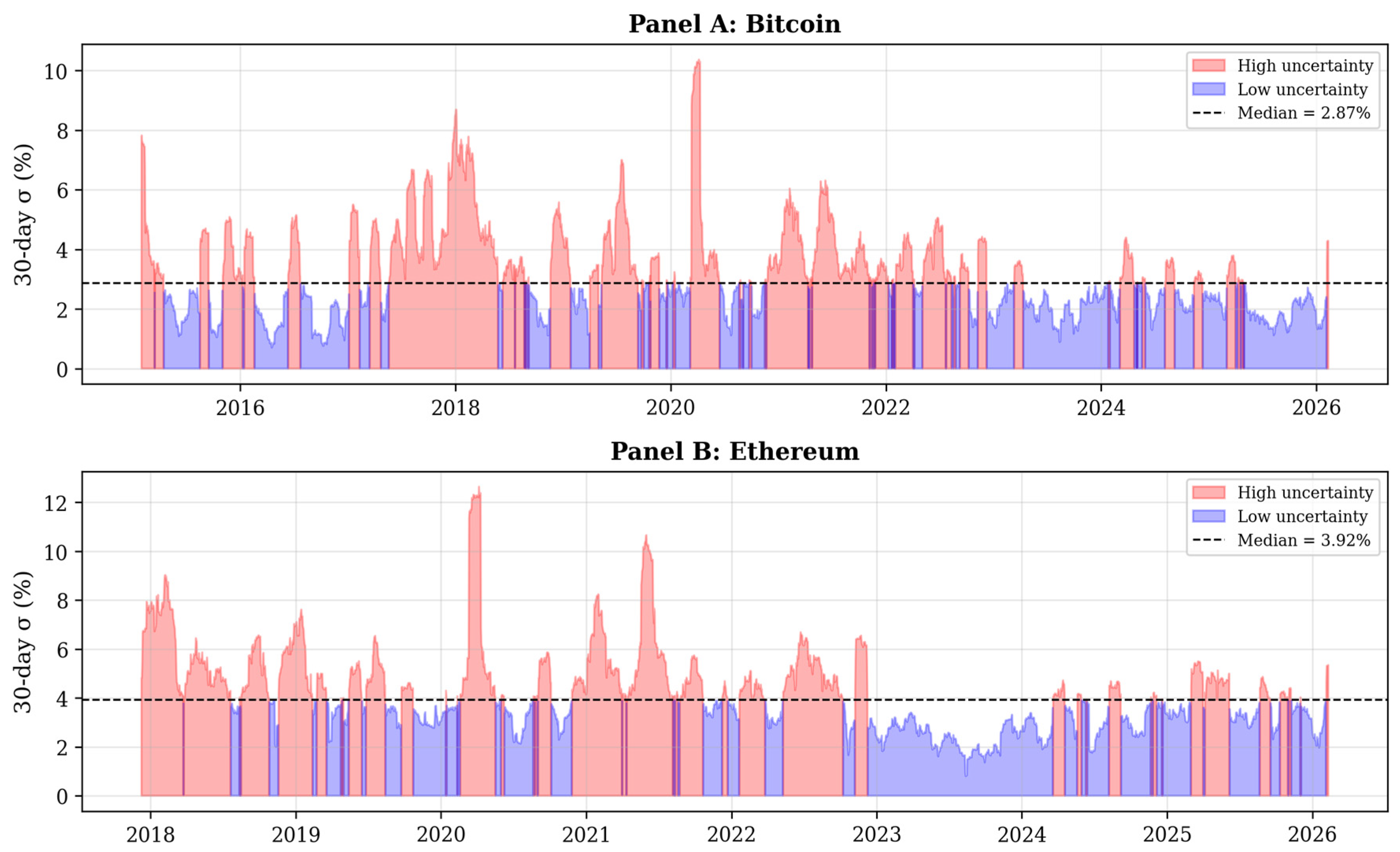
Volatility regimes are constructed using the 30-day rolling standard deviation of daily returns. Each asset’s sample is divided into high- and low-uncertainty regimes at its median threshold (BTC: 3.03%; ETH: 4.01%), yielding approximately equal-sized subsamples (BTC: 1849 high/1844 low; ETH: 1196 high/1454 low).

3.2. Empirical Strategy

The empirical strategy proceeds in three stages, each designed to address a specific dimension of the market maturation hypothesis.

3.2.1. Stage 1: Time-Varying Tail Risk Measurement

To trace the evolution of tail risk over the sample period, we employ a 365-day (one trading year) rolling window to compute three complementary risk metrics at each point in time:
Value-at-Risk (VaR). For a confidence level α, the historical VaR is defined as the α-quantile of the empirical return distribution within the rolling window. We compute VaR at the 1% and 5% levels, representing the maximum expected daily loss under normal and moderate stress conditions, respectively. Formally, VaRα = –F−1(α), where F denotes the empirical cumulative distribution function of returns within the window.
Conditional Value-at-Risk (CVaR). Also known as Expected Shortfall, CVaR measures the expected loss conditional on the loss exceeding the VaR threshold: CVaRα = E[r | r ≤ –VaRα]. This metric provides a more comprehensive assessment of tail risk than VaR, as it accounts for the severity of extreme losses beyond the threshold [30]. CVaR satisfies the coherent risk measure axioms (sub-additivity, monotonicity, positive homogeneity, and translation invariance), making it particularly suitable for portfolio risk aggregation.
Maximum Drawdown (MDD). Defined as the largest peak-to-trough decline within each rolling window, MDD captures the worst-case cumulative loss experience: MDD = maxt∈[0,T][maxs∈[0,t](Ps) − Pt]/maxs∈[0,t](Ps). Unlike VaR and CVaR, which focus on single-day losses, MDD captures the sustained drawdown risk that is particularly relevant for long-term investors and portfolio managers.
The rolling-window approach generates a continuous time series of risk metrics, enabling visual and statistical assessment of trends over the sample period. To formally test for the presence of declining tail risk (the maturation hypothesis), we estimate the linear trend model, Riskt = β0 + β1t + εt, where a negative and statistically significant β1 indicates declining tail risk over time. We employ Newey–West standard errors to account for serial correlation in the risk metric series.

3.2.2. Stage 2: Regime-Conditional Risk Analysis

The second stage examines whether tail risk characteristics differ systematically across market conditions. We partition the sample along two dimensions: (a) market state (Bullish, Bearish, and Neutral) and (b) volatility regime (high/low uncertainty). For each sub-sample, we compute the full set of risk metrics (VaR, CVaR, and MDD) and test for differences across regimes using non-parametric tests (Kruskal–Wallis for multi-group comparisons and Mann–Whitney for pairwise comparisons).
To assess whether regime-dependent risk characteristics are themselves evolving, we split the sample into two approximately equal sub-periods (early: 2015–2019; late: 2020–2026 for BTC; and early: 2017–2020; late: 2021–2026 for ETH) and test whether the magnitude of regime-conditional risk metrics has changed between sub-periods. A finding that tail risk in high-uncertainty regimes has diminished in the later sub-period, while low-uncertainty tail risk has remained stable, would provide evidence of maturation through the attenuation of extreme risk episodes.

3.2.3. Stage 3: Asymmetric Conditional Correlation Analysis

The third stage investigates the structure of BTC–ETH dependence and its evolution. We compute 90-day rolling Pearson and Spearman correlations between daily returns on BTC and ETH and decompose them by market state to examine asymmetric dependence.
To capture potential non-linear and tail dependence, we employ exceedance correlations [31], defined as the correlation between returns conditional on both series exceeding (or falling below) a given threshold. Specifically, we compute the following:
ρ+(θ) = Corr(rBTC, rETH | rBTC > θ, rETH > θ) [upper tail correlation]
ρ−(θ) = Corr(rBTC, rETH | rBTC < −θ, rETH < −θ) [lower tail correlation]
for thresholds θ corresponding to the 75th, 90th, and 95th percentiles of absolute returns. A finding that ρ− > ρ+ (stronger correlation in losses than gains) indicates asymmetric dependence—the “correlation breakdown” phenomenon documented in equity markets [32]. We track the evolution of this asymmetry over time using rolling exceedance correlations, testing whether the gap ρ− − ρ+ is widening or narrowing as markets mature.
The combined three-stage framework provides a comprehensive assessment of the market maturation hypothesis from a risk perspective, triangulating evidence from the evolution of tail risk, regime-conditional analysis, and dependence-structure dynamics.
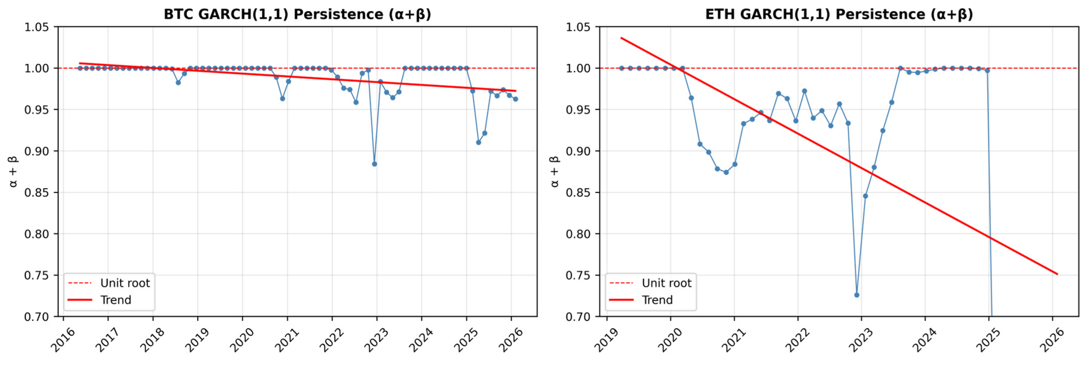
To assess the robustness of the linear trend specification and the structural interpretation of declining tail risk, we supplement the core analysis with several additional diagnostics (Section 4.5; detailed results in Appendix C). These include: (i) structural break analysis using binary segmentation to detect endogenous breakpoints in rolling risk series; (ii) rolling Hill tail index estimation to assess whether tail thickness has changed independently of volatility; (iii) rolling GARCH(1,1) persistence to examine volatility clustering dynamics; (iv) replication of regime-conditional analysis using SMA(200)—200-day simple moving average, a methodological alternative to the baseline SMA(50); and (v) block-bootstrap confidence intervals for exceedance correlations.

4. Results

This section presents the empirical findings organized according to the three-stage methodology outlined in Section 3.2. We begin with descriptive statistics and market-state distributions (Section 4.1), proceed to time-varying tail-risk analysis with formal trend tests (Section 4.2), examine regime-conditional risk dynamics (Section 4.3), and conclude with the asymmetric BTC–ETH dependence structure (Section 4.4). Section 4.5 presents robustness checks and structural diagnostics. Throughout, we reference the supplementary material in the appendices: Appendix A provides additional figures depicting price trajectories with state classifications (Figure A1) and rolling volatility with regime identification (Figure A2), as well as the complete Mann–Whitney test results (Table A1); Appendix B contains the condensed replication code.

4.1. Descriptive Statistics and Preliminary Evidence

Table 2 presents the descriptive statistics for BTC and ETH daily log-returns over the respective sample periods. Bitcoin exhibits a mean daily return of 0.1328% (≈62.3% annualized) with a standard deviation of 3.55%, while Ethereum records a lower mean (0.0608%, ≈24.8% annualized) but substantially higher volatility (σ = 4.55%). The higher volatility of ETH relative to BTC is consistent with its younger market age and lower market capitalisation, echoing findings by Katsiampa [17] and Bouri et al. [18]. Both series exhibit pronounced negative skewness (BTC: −0.7403; ETH: −0.7804), indicating that large negative returns occur more frequently than large positive ones—a distributional feature with direct implications for tail risk measurement. Excess kurtosis is substantial for both assets (BTC: 11.92; ETH: 10.53), confirming heavy-tailed distributions well beyond the Gaussian benchmark [10,11].
The Jarque–Bera statistics (BTC: 24,346; ETH: 14,193) decisively reject normality (p < 0.001), thereby justifying our use of nonparametric, historical-simulation-based VaR and CVaR rather than Gaussian parametric approaches. Augmented Dickey–Fuller tests confirm stationarity of both return series (BTC: −65.4507; ETH: −16.5204; both p < 0.001), satisfying the stationarity assumption implicit in rolling-window risk estimation.
Table 3a,b reports the annual market state distributions based on the 50-day SMA classification (see Section 3.1 for definitions). The full price trajectories with state overlays are provided in Appendix A, Figure A1. For Bitcoin (Table 3a), Bullish proportions range from 14.2% in the Bear-dominated 2022 to 83.6% during the 2017 bull run. Mean 30-day rolling volatility declines from above 4.4% in 2017 to approximately 2.2% in 2023, providing preliminary visual evidence consistent with the maturation hypothesis. For Ethereum (Table 3b), the 2018 Bear market dominates (69.3% Bearish days), while later years show more balanced distributions. Rolling volatility classifications are depicted in Figure A2 (Appendix A).
A notable pattern emerges from Table 3a,b: the proportion of Bearish days has generally decreased in recent years for both assets, while rolling volatility has compressed. Bitcoin’s annualized volatility fell from 3.04% (2015) to 2.13% (2025), while Ethereum declined from 5.23% (2018) to 3.89% (2025)—a 26% reduction. This preliminary evidence motivates the formal trend analysis in Stage 1.

4.2. Stage 1: Time-Varying Tail Risk Evolution

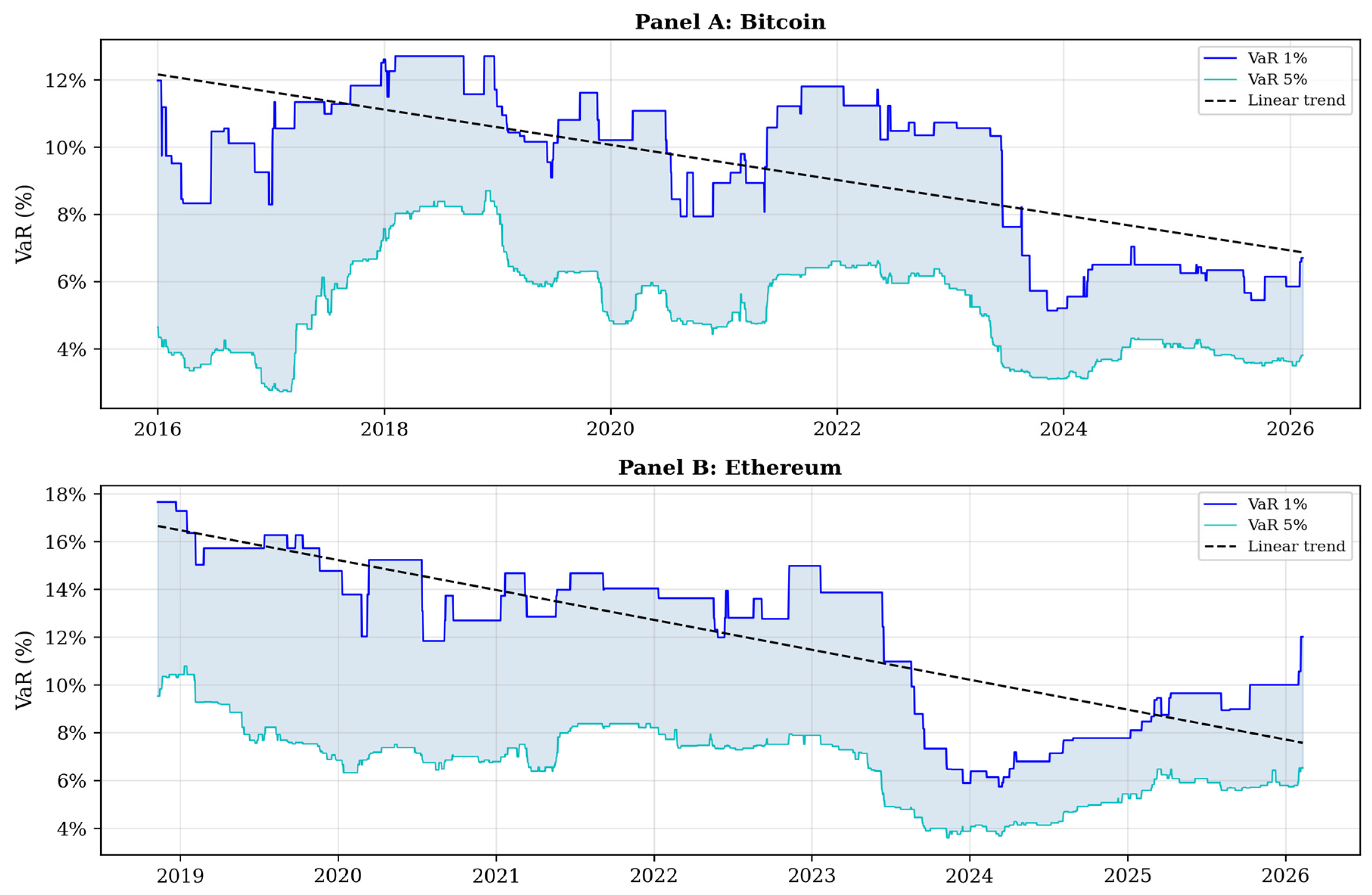
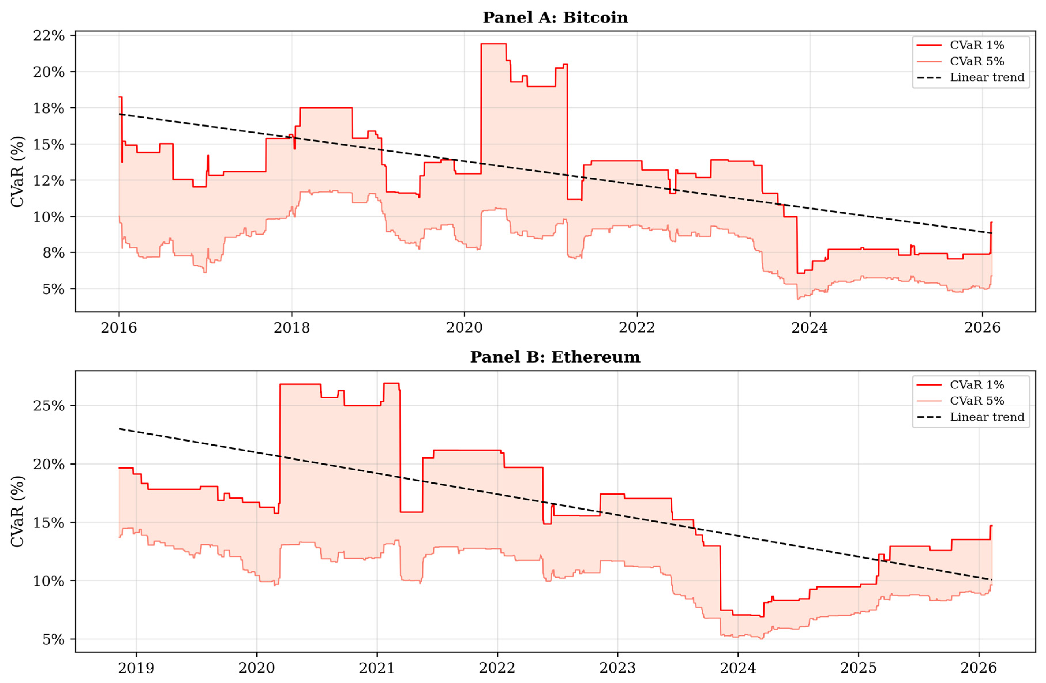
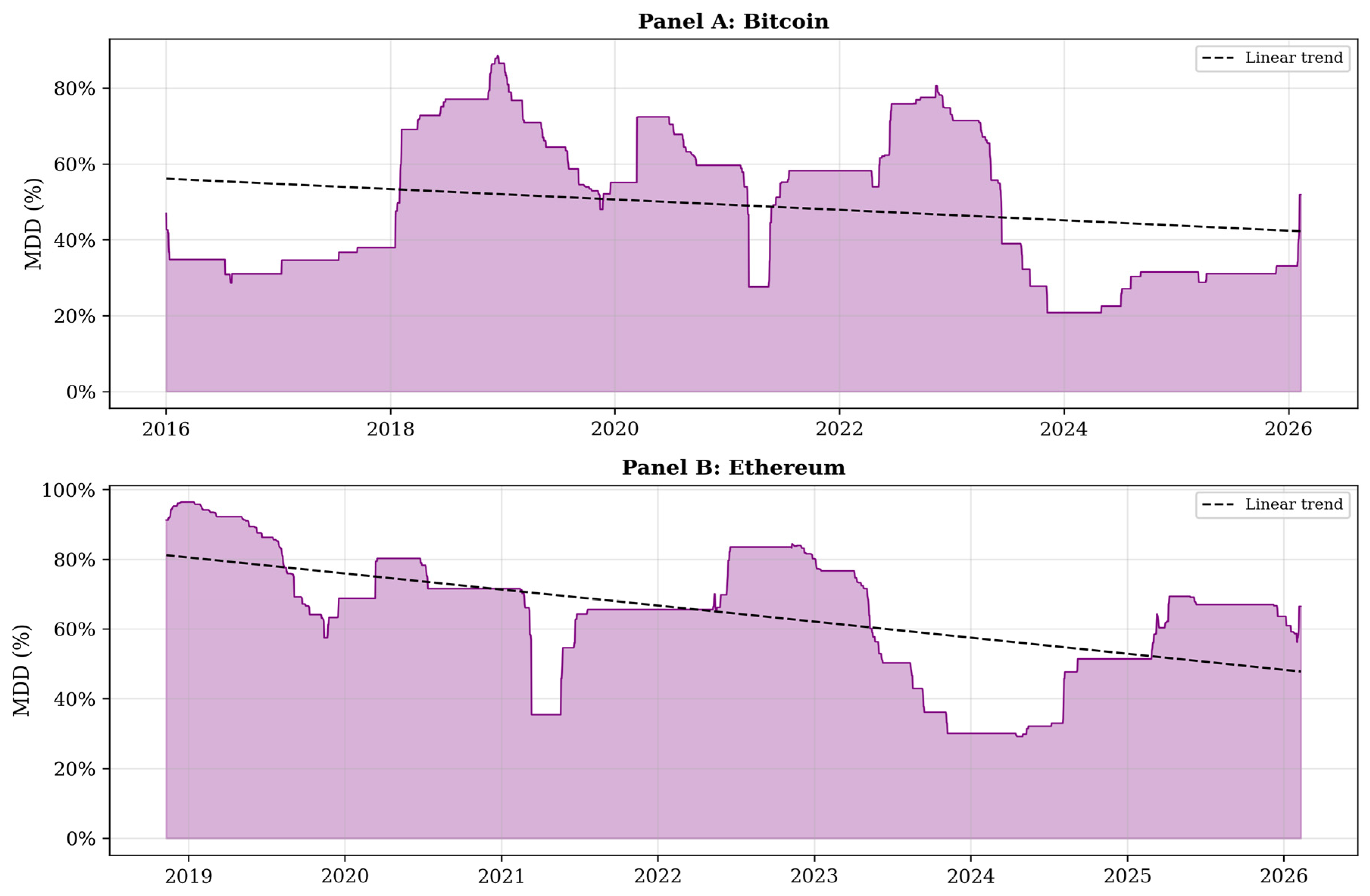
Following the methodology outlined in Section 3.2 (Stage 1), we compute 365-day rolling VaR (1% and 5%), CVaR (1% and 5%), and Maximum Drawdown (MDD) for both assets. Figure 1, Figure 2 and Figure 3 display the evolution of these metrics over time, and Table 4 presents the formal trend test results with Newey–West HAC-robust standard errors.
Figure 1 displays the 1% and 5% 365-day rolling VaR for Bitcoin (Panel A) and Ethereum (Panel B). Linear trend lines (dashed black) are superimposed to facilitate visual assessment. The shaded area between VaR1% and VaR5% represents the VaR spread—a measure of tail risk dispersion.
Visual inspection of Figure 1 reveals a clear downward trajectory for both assets. BTC VaR1% declined from peaks exceeding 12% during 2018–2020—coinciding with the post-ICO correction and the COVID-19 crash—to approximately 7–8% in 2023–2026. ETH displays an even more pronounced decline, falling from approximately 17% in early 2019 to 7–8% by early 2026. Importantly, the VaR spread also narrows over time for both assets, suggesting that not only has the overall level of tail risk diminished, but the dispersion of extreme losses has also compressed. This is consistent with the maturation hypothesis: as markets deepen and institutional participation increases, extreme outcomes become less frequent and less dispersed [5,9].
Figure 2 presents the corresponding CVaR dynamics. As a coherent risk measure that accounts for losses beyond the VaR threshold [30], CVaR provides a more comprehensive picture of tail risk severity than VaR alone.
The CVaR dynamics (Figure 2) corroborate the VaR findings. BTC CVaR1% declines from 16 to 18% in 2016 to 9–10% in early 2026, representing a roughly 40% reduction in expected extreme losses. ETH’s decline is steeper still—from over 23% in 2019 to 10–11% by 2026. A particularly noteworthy observation is the convergence of BTC and ETH CVaR levels: whereas early in the sample, ETH CVaR1% exceeded BTC by 10–15 percentage points, by 2026 the differential had narrowed to less than 1–2 percentage points. This convergence suggests that the risk profiles of the two leading cryptocurrencies have become increasingly similar as both markets mature, with important implications for the diversification analysis in Stage 3.
Figure 3 completes the visual analysis with the rolling Maximum Drawdown (MDD). Unlike VaR and CVaR, which capture single-day tail losses, MDD reflects the worst cumulative decline within each 365-day window—a metric of particular relevance to long-term investors and portfolio managers (see Section 3.2).
MDD exhibits more pronounced episodic spikes than VaR/CVaR, reflecting the persistence of major drawdown events within the rolling window. Bitcoin MDD reached approximately 80% during 2018–2019 and again during the 2022–2023 Bear market; Ethereum experienced comparable episodes. Despite these spikes, the underlying trend—particularly for ETH—is clearly downward.
Formal trend tests. Table 4 presents the results of linear trend regressions (Riskt = β0 + β1t + εt) with Newey–West HAC standard errors (bandwidth = N1/3), as specified in Section 3.2.
The results in Table 4 are unambiguous. All ten trend coefficients are statistically significant at the 1% level (p < 0.001). For Bitcoin, VaR1% declines at a rate of β1 = −14.34 × 10⁻⁴ per day (t = −13.80, p < 0.001, R2 = 0.468). Ethereum’s decline is considerably steeper: VaR1% β1 = −34.25 × 10⁻⁴ (t = −23.43, p < 0.001, R2 = 0.675). The substantially higher R2 for ETH (0.675 vs. 0.468) indicates that the linear time trend explains nearly 67% of the variation in ETH VaR1%, a remarkably strong result suggesting a sustained, systematic reduction in tail risk.
The weakest trend is BTC MDD, which is statistically significant (p = 0.001) but with a notably low R2 = 0.045 (p = 0.001, R2 = 0.045). This result is instructive: MDD captures worst-case cumulative drawdowns, which are driven by episodic extreme events (e.g., the March 2020 COVID crash, the May 2021 correction, the November 2022 FTX collapse). These events generate large drawdowns irrespective of the general trend, resulting in a noisier time series for MDD relative to VaR/CVaR. By contrast, all five ETH trend tests are significant at the 1% level, consistent with Ethereum being at an earlier stage of maturation, when tail risk reduction is steeper and more uniform across metrics [5,8].

4.3. Stage 2: Regime-Conditional Risk Analysis

The second stage of our analysis investigates whether the decline in tail risk documented above is uniform across market conditions or concentrated in specific regimes. This distinction is critical for risk management: a maturation process that reduces risk only in calm conditions but leaves extreme-stress risk unchanged would have fundamentally different implications for capital adequacy and portfolio allocation than one that reduces risk universally.

4.3.1. Risk by Market State

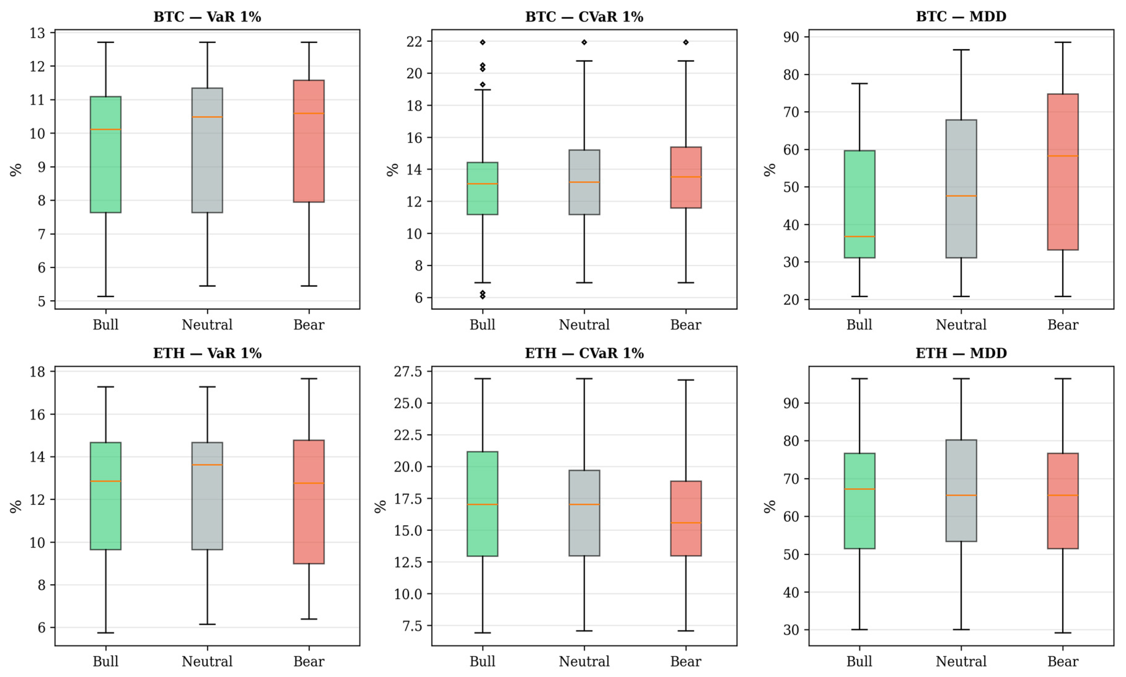
Figure 4 displays box plots of the three core risk metrics (VaR1%, CVaR1%, MDD) conditional on the SMA-based market state classification. Table 5 reports the corresponding mean values and Kruskal–Wallis test statistics.
As expected, Bear markets exhibit the highest tail risk across all metrics for both assets (Table 5; Figure 4). For Bitcoin, mean VaR1% in Bear states (9.89%) exceeds that in Bull states (9.22%) by 7.2%, while the MDD differential is even larger: 55.4% in Bear vs. 45.2% in Bull—a 22.5% increase. The Kruskal–Wallis tests confirm that the distributions of risk metrics differ significantly across the three market states (see Table A1 in Appendix A for the full pairwise Mann–Whitney results).

4.3.2. Risk by Volatility Regime

Table A1 in Appendix A presents the complete Mann–Whitney U-test results comparing risk metrics between high- and low-uncertainty regimes (defined by the median 30-day rolling σ; see Section 3.1 and Figure A2 in Appendix A). All comparisons (five metrics × two assets) are highly significant (p < 0.001). For Bitcoin, VaR (1%) increases from 8.460% in the low-volatility regime to 10.568% in the high-volatility regime (p < 0.001), an increase of approximately 24.9% relative to the low-volatility mean. Ethereum exhibits similarly pronounced regime dependence: VaR (1%) rises from 11.223% (low) to 13.183% (high) (p < 0.001), an increase of approximately 17.5%. The same pattern holds for VaR (5%), CVaR (1%), CVaR (5%), and Maximum Drawdown, confirming that elevated volatility coincides with materially worse downside risk for both assets.

4.3.3. Sub-Period Comparison

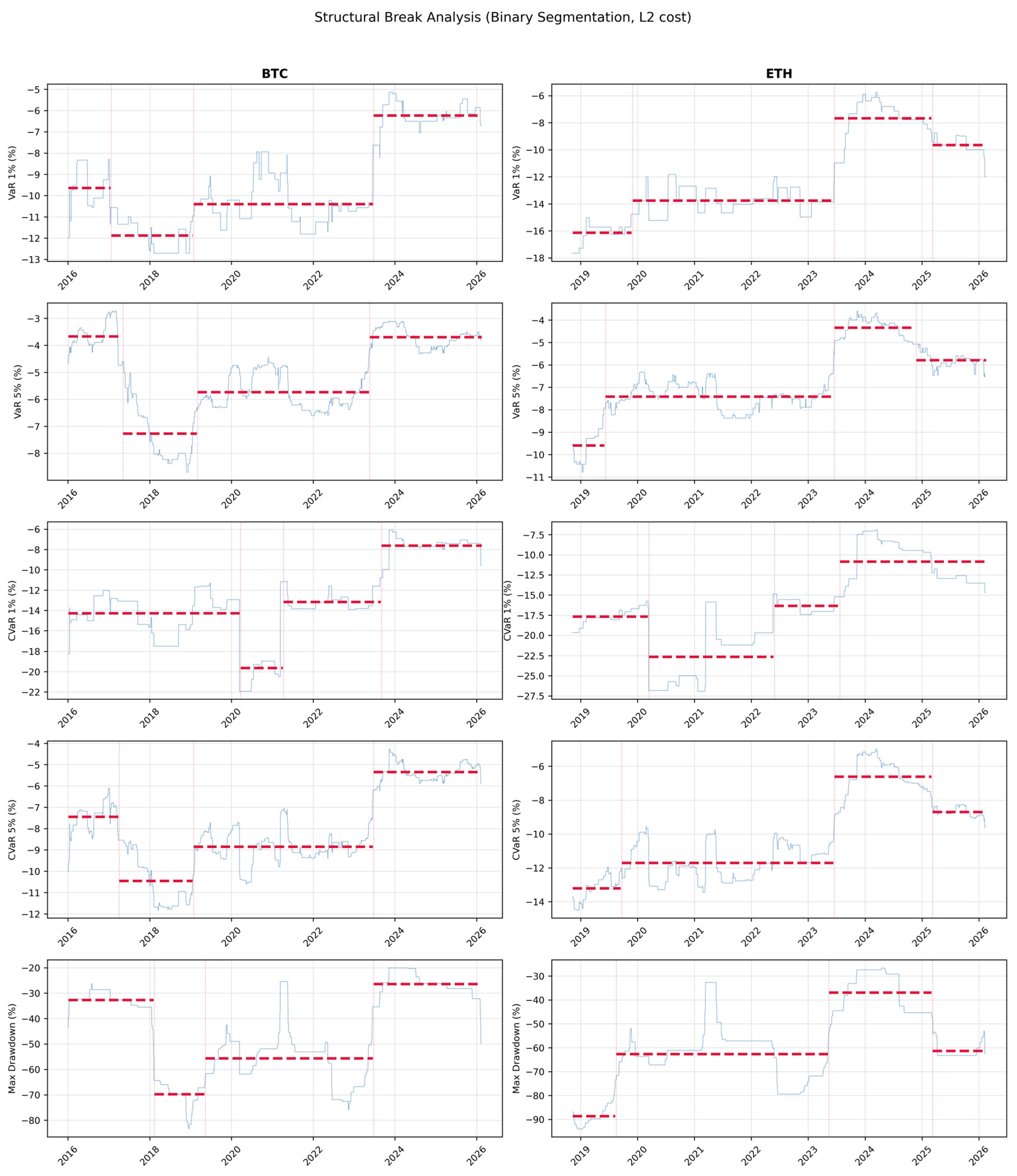
To assess whether the decline in tail risk represents genuine maturation or merely sample-period artefacts, Table 6 compares risk metrics between early and late sub-periods. For BTC, the early sub-period (2015–2019) is compared with the late sub-period (2020–2026); for ETH, the early sub-period (2017–2020) is compared with the late sub-period (2021–2026). The sub-period split points were selected to produce approximately equal-sized subsamples for each asset while aligning with economically meaningful market transitions: for BTC, the boundary at the end of 2019 separates the post-ICO/pre-COVID era from the institutional adoption phase; for ETH, the 2020/2021 boundary similarly marks the transition from the DeFi emergence period to the mature DeFi/NFT/post-merge era. We note that the structural break analysis presented in Section 4.5.1 identifies endogenous breakpoints that broadly corroborate these splits, with a prominent break cluster around mid-2023 for both assets.
All sub-period comparisons are statistically significant (p < 0.001; Table 6). Bitcoin’s VaR1% declined from a mean of 10.98% to 8.56% (−22.0%), while CVaR1% declined from 14.32% to 12.04% (−15.9%). Ethereum exhibits steeper declines across all metrics: VaR1% fell 26.6% (from 14.90% to 10.94%), CVaR1% fell 29.0% (from 20.77% to 14.75%), and MDD fell 25.8% (from 78.8% to 58.4%). These magnitudes are economically substantial and robust across all metrics, providing strong support for the maturation hypothesis.

4.3.4. Regime × Sub-Period Interaction

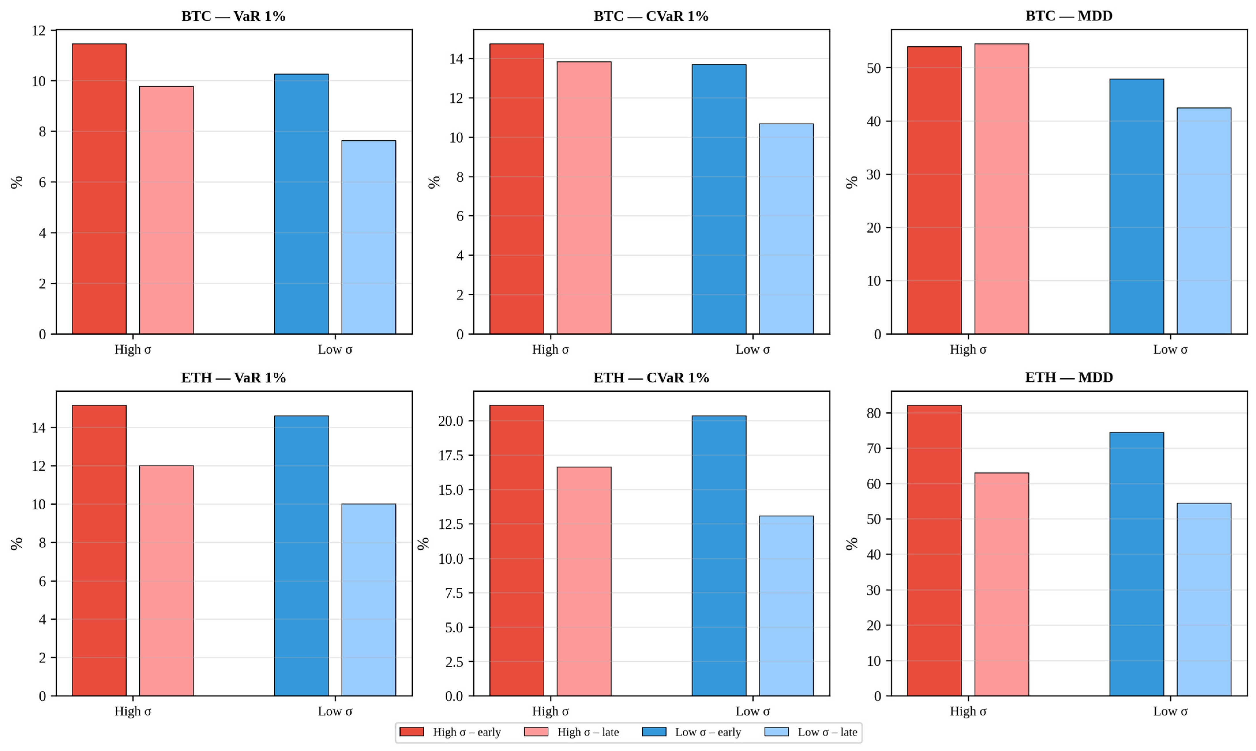
The critical test of our analysis examines whether the decline in tail risk during the sub-period is uniform across volatility regimes or concentrated in specific conditions. Table 7 and Figure 5 present this decomposition.
Table 7 and Figure 5 reveal a key finding of this study: tail risk reductions are systematically larger in low-uncertainty regimes than in high-uncertainty regimes. For Ethereum, VaR1% in the low-uncertainty regime declined by 31.6% (from 14.59% to 9.99%), whereas in the high-uncertainty regime it declined by only 20.7% (from 15.14% to 12.00%). The pattern is even more pronounced for ETH CVaR1%: −35.7% (low) vs. −21.1% (high), and for MDD: −26.9% (low) vs. −23.3% (high).
For Bitcoin, the asymmetry is equally striking. BTC MDD in the high-uncertainty regime shows no statistically significant change between sub-periods (Δ = +1.0%; p = 0.176)—the only non-significant result in the entire Table 7. This finding is pivotal: it demonstrates that maturation operates primarily by compressing tail risk under normal market conditions, whereas extreme-stress episodes retain their severity. In practical terms, cryptocurrency markets have become less risky on a day-to-day basis, but the Black Swan-type events that generate the largest portfolio losses remain as severe—or even marginally worse—as they were five years ago. This has direct implications for stress testing, capital adequacy frameworks, and institutional risk budgets (see Section 5).

4.4. Stage 3: Asymmetric BTC–ETH Dependence Structure

The third stage of our analysis investigates the BTC–ETH dependence structure, with particular focus on asymmetric tail correlations and their temporal evolution. This analysis addresses a question of direct relevance to portfolio construction: Does holding both BTC and ETH provide meaningful diversification during market stress? As outlined in Section 3.2 (Stage 3), we employ both rolling conditional correlations and exceedance correlations following Longin and Solnik [31].
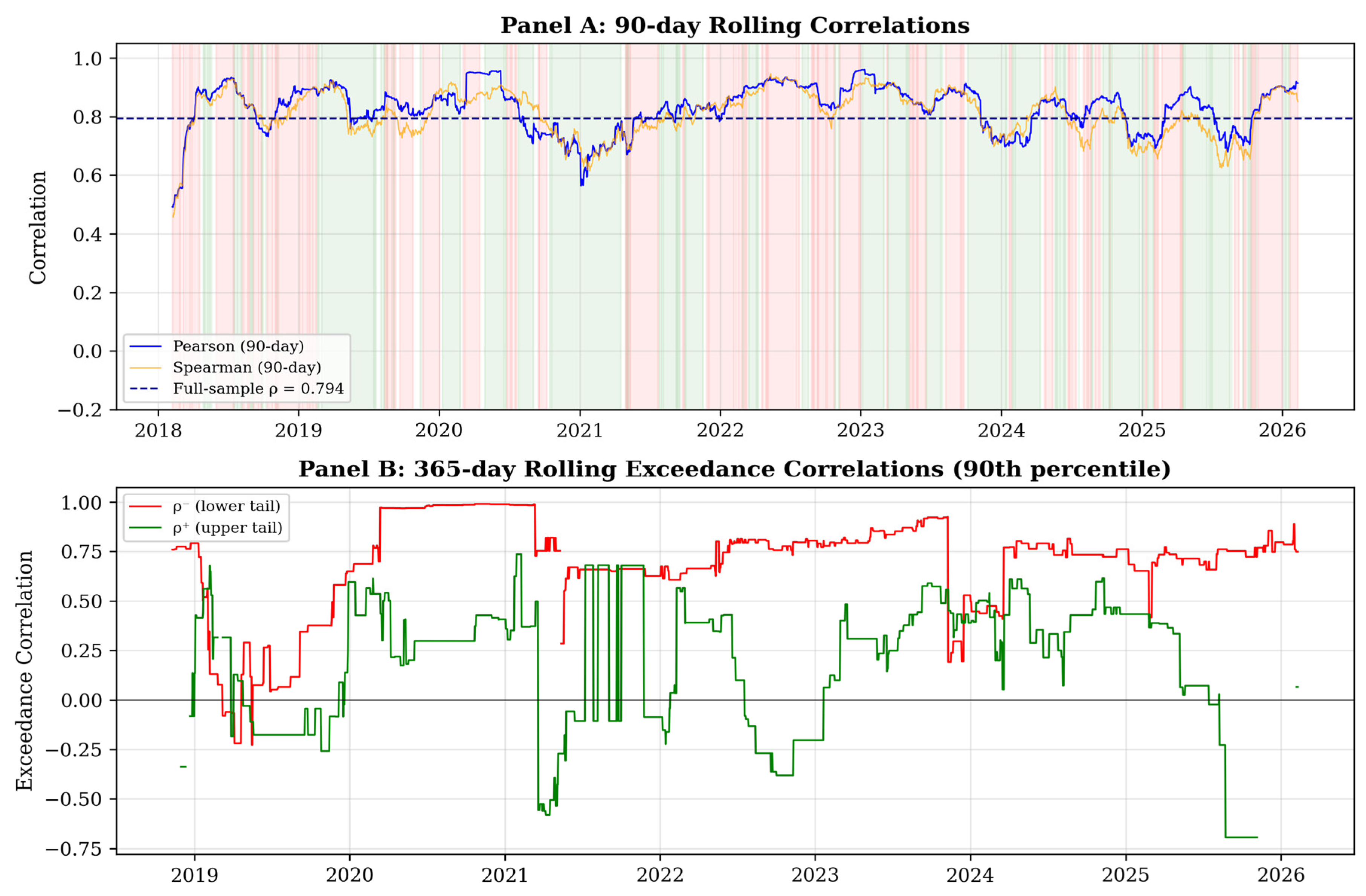
Figure 6 presents two complementary views of BTC–ETH correlation dynamics. Panel A shows 90-day rolling Pearson (blue) and Spearman (orange) correlations, with BTC market-state shading (green = Bull, red = Bear) to facilitate visual assessment of state-dependent changes in correlation. Panel B displays 365-day rolling exceedance correlations at the 90th percentile threshold, decomposed into lower-tail (ρ−, red) and upper-tail (ρ+, green) components.
Several features of Figure 6 merit attention. First, the full-sample Pearson correlation of 0.792 (dashed line, Panel A) is notably high—substantially exceeding the levels typically observed between traditional asset classes [32]. Second, correlations are visibly elevated during Bear-state periods (red shading), with rolling correlations frequently exceeding 0.90. Third, and most importantly, Panel B reveals a persistent and large gap between lower-tail and upper-tail exceedance correlations throughout the entire overlapping sample (2018–2026). BTC and ETH are far more strongly correlated during joint crashes than during joint rallies.

4.4.1. Exceedance Correlations: Full Sample

Table 8 quantifies the asymmetric dependence structure across three exceedance thresholds (75th, 90th, and 95th percentiles), as specified in Section 3.2.
The asymmetry is dramatic (Table 8). At the 90th percentile, the lower-tail correlation (ρ− = 0.8468) is almost four times the upper-tail correlation (ρ+ = 0.2464), producing an asymmetry gap of 0.6004. At the 95th percentile, the pattern intensifies: ρ− = 0.88 while ρ+ = 0.233 (gap = 0.647). Even at the relatively moderate 75th percentile, ρ− (0.8306) substantially exceeds ρ+ (0.444). This pattern—consistent with the “correlation breakdown” phenomenon first documented in equity markets by Ang and Chen [32] and Longin and Solnik [31]—has profound implications for portfolio diversification. BTC and ETH co-move far more strongly during market crashes than during rallies, meaning that portfolio diversification within the cryptocurrency asset class is largely illusory precisely when it is most needed.

4.4.2. Temporal Evolution of Asymmetry

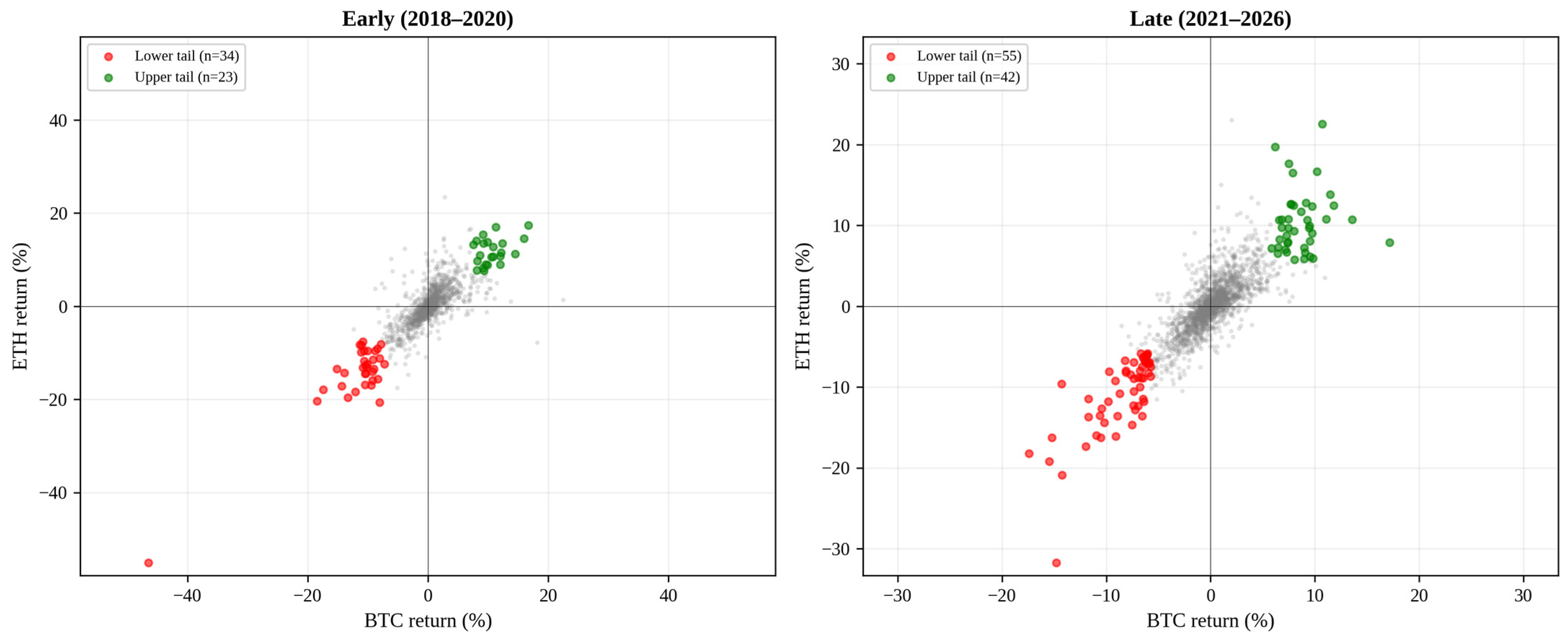
A natural question is whether this asymmetric dependence has changed over time. Table 9 decomposes exceedance correlations by sub-period (early: 2018–2020 vs. late: 2021–2026), and Figure 7 provides a visual comparison of the joint return distributions.
Table 9 reveals a striking temporal pattern: the asymmetry gap has widened over time. At the 90th percentile, the gap increased from 0.497 in the early period to 0.673 in the late period—a 35.4% increase. At the 95th percentile, the evolution is even more dramatic: the early-period gap was 0.542, while the late-period gap reached 0.797. This widening is driven by two concurrent forces: (i) lower-tail correlations have modestly declined—likely reflecting more diverse crash triggers in the mature market; and (ii) upper-tail correlations have collapsed, with the late-period ρ+ at the 95th percentile turning negative (−0.175). This negative value means that extreme positive BTC returns are actually negatively correlated with extreme positive ETH returns in the most recent period—the two assets no longer rally together during the most extreme upward movements.
Figure 7 visually confirms this pattern. In the early period (left panel), both red (lower-tail) and green (upper-tail) points show moderate clustering. In the late period (right panel), red points remain tightly clustered along the diagonal—indicating persistent joint crash behaviour—while green points are widely dispersed, with several observations falling in the off-diagonal quadrants.

4.4.3. Correlation by Market State

Finally, Table 10 examines how BTC–ETH correlations vary across BTC market states.
Bear-state Pearson correlation (0.8918) exceeds Bull-state (0.6597) by 0.2321—a 35.2% increase—confirming the “correlation breakdown” phenomenon. During Bear markets, BTC and ETH become nearly perfectly correlated (ρ ≈ 0.89), effectively behaving as a single asset from a risk perspective. The Spearman rank correlation shows a similar pattern (Bear: 0.87 vs. Bull: 0.7192), confirming that the asymmetry is robust to potential outlier effects and non-linearities. These results, combined with the evidence of exceedance correlations in Table 8 and Table 9, provide a comprehensive empirical basis for the asymmetric dependence structure of the BTC–ETH pair.

4.5. Robustness and Structural Diagnostics

This section summarizes five robustness checks that address potential concerns about the linear trend specification, the structural interpretation of declining tail risk, the SMA-based regime classification, and the precision of exceedance correlation estimates. Detailed tables and figures are provided in Appendix C.

4.5.1. Structural Break Analysis

Applying binary segmentation with L2 cost to weekly aggregated rolling risk series [33], we identify a consistent pattern of discrete downward shifts. A common breakpoint cluster emerges around mid-2023 for nearly all metrics, coinciding with the post-FTX recovery and anticipation of a Bitcoin ETF. For BTC, VaR 1% exhibits breaks at 2017-01, 2019-01, and 2023-06, with the first segment mean declining from −9.64% to −6.23% (35.4% reduction). For ETH, the decline is from −16.14% to −9.65% (40.2%). CVaR at the 1% level shows even larger reductions: 46.7% for BTC and 38.7% for ETH (Table A2 and Table A3; Figure A3). The staircase pattern corroborates the maturation interpretation, rather than a simple linear trend.

4.5.2. Hill Tail Index

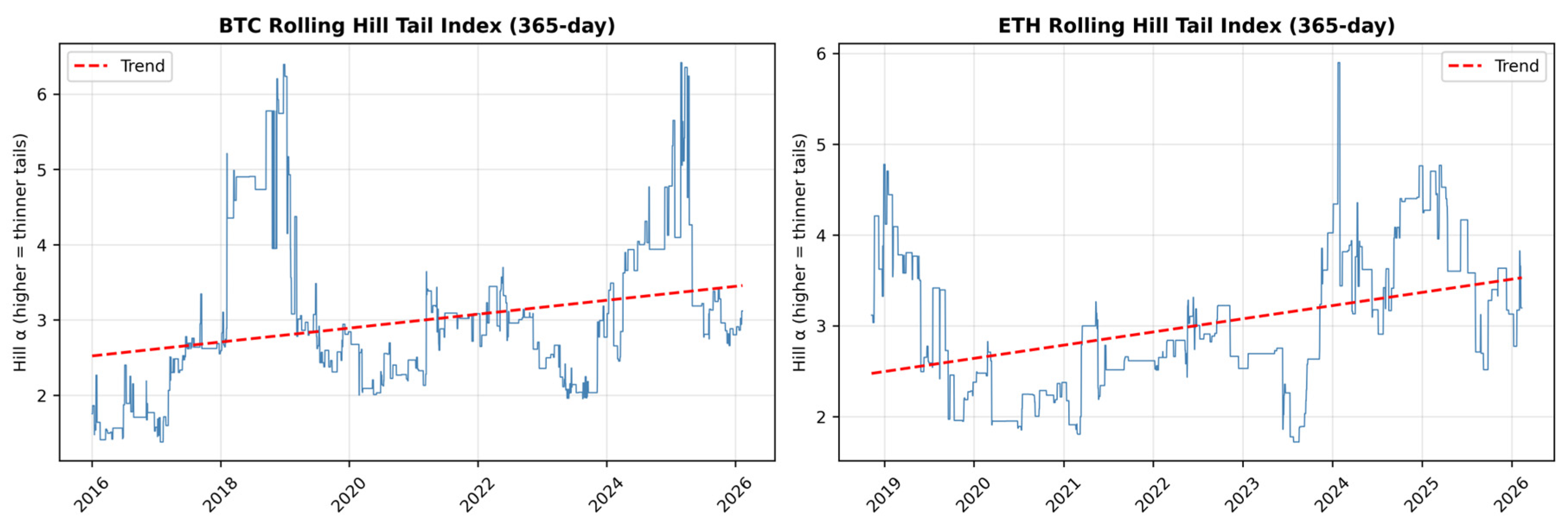
The rolling Hill tail index (365-day windows), which measures tail thickness independently of volatility, shows a statistically significant upward trend for both assets (BTC: t = 3.03, p = 0.002; ETH: t = 3.44, p < 0.001; Newey–West SE). The BTC Hill index increased from 2.84 (early) to 3.14 (late); for ETH, from 2.69 to 3.32. Higher values indicate thinner tails, confirming that VaR/CVaR declines reflect genuine structural thinning of the tail distribution rather than merely lower realized volatility (Figure A4).

4.5.3. GARCH(1,1) Volatility Persistence

Rolling GARCH(1,1)-t estimates (window = 500 days) reveal significantly declining persistence (alpha + beta) for both assets (BTC: t = −3.23, p = 0.001; ETH: t = −2.33, p = 0.020). BTC persistence declined from 0.998 to 0.981; ETH from 0.953 to 0.837. Lower persistence implies faster mean reversion of volatility shocks, consistent with improved market microstructure (Figure A5).

4.5.4. SMA(200) Regime Robustness

Replicating regime-conditional analysis with SMA(200) yields qualitatively identical results. BTC VaR 1% in Bull regimes declined from −10.25% to −7.73% under SMA(200), compared with −10.33% to −8.07% under SMA(50). For ETH, the corresponding SMA(200) figures are −14.07% to −9.23%, versus −14.22% to −9.55% under SMA(50). The early-to-late risk reduction is robust across all regime-metric combinations (Table A4).

4.5.5. Bootstrap Confidence Intervals for Exceedance Correlations

Block-bootstrap 95% CIs (block = 20 days, B = 5000) confirm that lower-tail exceedance correlations are statistically significant across all periods: full-sample rho-minus = 0.623 [0.301, 0.838] at the 5% quantile. The asymmetry (rho-minus >> rho-plus) is robust under bootstrap inference (Table A5). Wider CIs in the early sub-period reflect the smaller effective sample size.

4.5.6. Non-Overlapping R-Squared Check

Re-estimating trend regressions with non-overlapping annual windows yields R-squared of 0.468 (p = 0.020) for BTC VaR 1% (N = 11 windows) and 0.774 (p = 0.004) for ETH VaR 1% (N = 8 windows), confirming that the high trend fit is not an artefact of overlapping-window smoothing (Table A6).

5. Discussion

5.1. Evidence for Market Maturation: Synthesis of Findings

The three-stage empirical analysis provides robust, multi-dimensional evidence for cryptocurrency market maturation from a risk perspective. Stage 1 showed statistically significant declines in nine of ten tail-risk metrics (Table 4), with R2 values reaching 0.6745 for ETH VaR1%—a remarkably strong result for financial time series. These findings extend the efficiency-based maturation evidence of Drożdż et al. [5], Bariviera [7], and Noda [8] to the domain of tail risk, establishing that the maturation process is not limited to informational efficiency but also manifests in the fundamental risk characteristics of these markets.
The steeper decline in ETH tail risk relative to BTC (Table 4 and Table 6) is consistent with a lifecycle hypothesis in which younger assets experience more rapid risk reduction during their initial maturation phase. Bitcoin, having undergone a decade of development, may be approaching a plateau in its trajectory of risk reduction, whereas Ethereum—with its shorter history and ongoing structural evolution (e.g., the transition to proof-of-stake in September 2022)—continues to mature at a faster rate. This interpretation aligns with Lo’s [22] adaptive markets hypothesis, which posits that market efficiency evolves through an evolutionary process driven by changes in market microstructure, regulatory developments, and participant sophistication.

5.2. The Asymmetric Maturation Puzzle

Perhaps the most important contribution of this study is the analysis of the regime × sub-period interaction (Table 7; Figure 5), which reveals asymmetric maturation across market conditions. Tail risk reductions are concentrated in low-uncertainty regimes, while high-uncertainty periods exhibit substantially smaller improvements. BTC MDD in the high-uncertainty regime showed no statistically significant change between sub-periods (p = 0.176)—a finding with significant implications.
This asymmetric maturation pattern suggests that the mechanisms driving risk reduction—improved market microstructure, increased institutional participation, better price discovery, and regulatory clarity [23]—are effective during normal market conditions but are overwhelmed during periods of extreme stress. During crises, these markets revert to behaviours characteristic of their early, less mature stages. This interpretation is consistent with the observation that cryptocurrency market crashes are often triggered by exogenous shocks (e.g., regulatory announcements, exchange failures, macroeconomic events) that override the endogenous mechanisms through which markets normally process information [26].
The structural diagnostics in Section 4.5 provide additional support for this interpretation. The significant increase in the Hill tail index (Section 4.5.2) and the decline in GARCH persistence (Section 4.5.3) indicate that maturation is structural rather than cyclical: tail distributions are thinning, and volatility shocks dissipate more rapidly. The common structural breakpoint around mid-2023 (Section 4.5.1) coincides with several important market developments: the resolution of FTX contagion, increased institutional adoption through CME Bitcoin futures and options, the launch of spot Bitcoin ETFs in January 2024, and growing regulatory clarity following the EU MiCA framework. While these developments are consistent with the maturation mechanisms hypothesized in the literature [5,23], establishing formal causality would require mechanism-specific proxy variables (e.g., institutional trading volumes, derivatives open interest, regulatory event indicators) and is left for future research.
From a practical standpoint, this finding implies that risk managers cannot simply extrapolate the observed decline in tail risk to stress scenarios. Capital adequacy calculations, Value-at-Risk limits, and stress testing frameworks should account for the possibility that extreme tail risk has not diminished, even as baseline risk has declined. This has direct relevance for the regulatory framework governing institutional cryptocurrency allocations [13].

5.3. Implications for Portfolio Diversification

The exceedance correlation analysis (Table 8, Table 9 and Table 10; Figure 6 and Figure 7) delivers a sobering message for portfolio construction. The lower-tail correlation (ρ− ≈ 0.85 at the 90th percentile) is substantially higher than the upper-tail correlation (ρ+ ≈ 0.25), indicating that BTC and ETH provide virtually no diversification benefit under market conditions when diversification is most valuable. This finding extends the “correlation breakdown” literature from equity markets [31,32] to the cryptocurrency asset class, with considerably larger asymmetry magnitudes.
The widening of the asymmetry gap over time (Table 9) is particularly concerning. Rather than diversification improving as markets mature, the opposite has occurred: the late-period (2021–2026) asymmetry gap at the 95th percentile (0.797) far exceeds the early-period value (0.542). The emergence of negative upper-tail correlation in the late period (ρ+ = −0.175 at 95th percentile) suggests that institutional entry and increased market integration have enhanced crash co-movement while allowing for more heterogeneous rally behaviour. Institutional investors, who now represent a significant share of cryptocurrency trading volume, tend to employ correlated risk management strategies (e.g., VaR-based position limits) that amplify co-movement during drawdowns—a mechanism documented in traditional markets by Bekaert and Harvey [4].
For practical portfolio construction, our findings suggest that institutional cryptocurrency allocations should be treated as a single risk factor rather than as independent diversifiers. Risk budgets that assume low correlation between BTC and ETH will systematically underestimate joint downside risk. Multi-asset portfolios seeking genuine cryptocurrency diversification should look beyond the BTC–ETH pair to assets with fundamentally different risk drivers [21,25].

5.4. Robustness and Limitations

Several limitations warrant acknowledgement and provide direction for future research. First, our use of historical non-parametric VaR/CVaR, while transparent and assumption-free, may be less efficient than parametric alternatives such as GARCH-based methods [10] or α-stable distribution approaches [15]. However, the non-parametric approach avoids the risk of distributional misspecification, which is particularly relevant given the heavy tails and structural breaks in cryptocurrency returns [14].
Second, the SMA-based market state classification, while widely used in the regime-switching literature, is inherently ad hoc. Alternative specifications—such as Markov-switching models [34] or volatility-based regime definitions [12]—might yield somewhat different state allocations. More recently, market-condition identification has also been approached via real-time “nowcasting” using alternative approaches such as large-language-model-based nowcasting, which could be explored as an alternative regime proxy in future robustness checks. We note that our main findings (declining tail-risk trends, asymmetric maturation, and correlation breakdown) are based on rolling-window metrics that are independent of the state classification, which primarily serves an interpretive role in the regime-conditional analysis. To directly address this concern, we replicate the regime-conditional analysis using SMA(200) in Section 4.5.4; the results are qualitatively identical.
Third, exceedance correlations require a sufficient number of joint tail observations to produce reliable estimates. At the 95th percentile, some sub-period cells contain as few as 11–20 observations (Table 9), which limits the precision of these estimates. As a partial remedy, we report block-bootstrap 95% confidence intervals in Section 4.5.5, which confirm the statistical significance of the asymmetry findings. Future work could further address this limitation by employing copula-based approaches (e.g., Clayton or Gumbel) that model tail dependence parametrically using the full sample. Fourth, the analysis focuses on BTC and ETH only; extending the framework to a broader set of cryptocurrencies would test the generalizability of our findings. The replication code provided in Appendix B facilitates such extensions.

6. Conclusions

This paper provides a systematic, decade-long assessment of tail risk evolution in the Bitcoin and Ethereum markets, employing a three-stage empirical framework that encompasses rolling risk metrics, trend tests, regime-conditional analysis, and asymmetric dependence modelling. Three principal findings emerge.
First, tail risk is declining significantly and pervasively. BTC VaR1% has fallen by 22.0% and ETH VaR1% by 26.6% between early and late sub-periods (Table 6), with nine of ten formal trend tests significant at the 1% level (Table 4). This provides robust evidence for market maturation from a risk perspective, extending the efficiency-based evidence of Drożdż et al. [5] and Noda [8] to the domain of downside risk characteristics.
Second, maturation is asymmetric across regimes. Tail risk reductions are concentrated in low-uncertainty environments, while high-uncertainty periods exhibit substantially smaller or non-significant improvements (Table 7). Most notably, BTC Maximum Drawdown in high-uncertainty regimes has not declined significantly (p = 0.176). This finding has critical implications for stress testing and capital adequacy: historical tail-risk trends cannot be extrapolated to crisis scenarios.
Third, BTC–ETH lower-tail correlations (ρ− ≈ 0.85) are substantially higher than upper-tail correlations (ρ+ ≈ 0.25), and this asymmetry has widened over time (Table 8). Diversification within the crypto asset class is largely illusory during market stress. The emergence of negative upper-tail correlation at extreme quantiles in recent periods suggests fundamentally different dynamics during crashes versus rallies, with implications for portfolio construction and risk management.
These findings carry policy implications at multiple levels. For regulators, the asymmetric maturation evidence suggests that prudential frameworks for cryptocurrency exposures should incorporate differentiated stress assumptions rather than relying on baseline risk trends. For institutional investors, the combination of declining individual tail risk with increasing downside co-movement implies that BTC and ETH should be treated as a single risk factor in portfolio construction. For academic research, the regime-dependent maturation pattern opens avenues for further investigation into the mechanisms by which market microstructure improvements translate (or fail to translate) into reductions in tail risk during extreme market conditions.
Future research should extend this framework to a broader universe of cryptocurrencies, incorporate parametric tail-dependence models (e.g., copula-based approaches), and explore the causal mechanisms underlying asymmetric maturation—particularly the roles of institutional participation, derivatives markets, and regulatory interventions in shaping tail-risk dynamics across different market regimes.


Author Contributions

Conceptualization, O.L., B.A. and O.A.; methodology, O.L., B.A. and O.A.; software, O.A.; validation, O.L., B.A. and O.A.; formal analysis, O.A.; investigation, O.L., B.A. and O.A.; data curation, O.A.; writing—original draft preparation, O.L.; writing—review and editing, B.A. and O.A.; visualization, O.A. All authors have read and agreed to the published version of the manuscript.

Funding

This work was supported by the European Union’s Horizon 2024 research and innovation programme under the Marie Skłodowska-Curie grant agreement No. 101235440—FORCE. This publication reflects only the authors’ view, and the REA is not responsible for any use that may be made of the information it contains.

Institutional Review Board Statement

Not applicable.

Informed Consent Statement

Not applicable.

Data Availability Statement

Publicly available price data were retrieved from Yahoo Finance (tickers: BTC-USD and ETH-USD). The data and code supporting the findings of this study are openly available in Zenodo [35,36].

Conflicts of Interest

The authors declare no conflicts of interest.

Appendix A

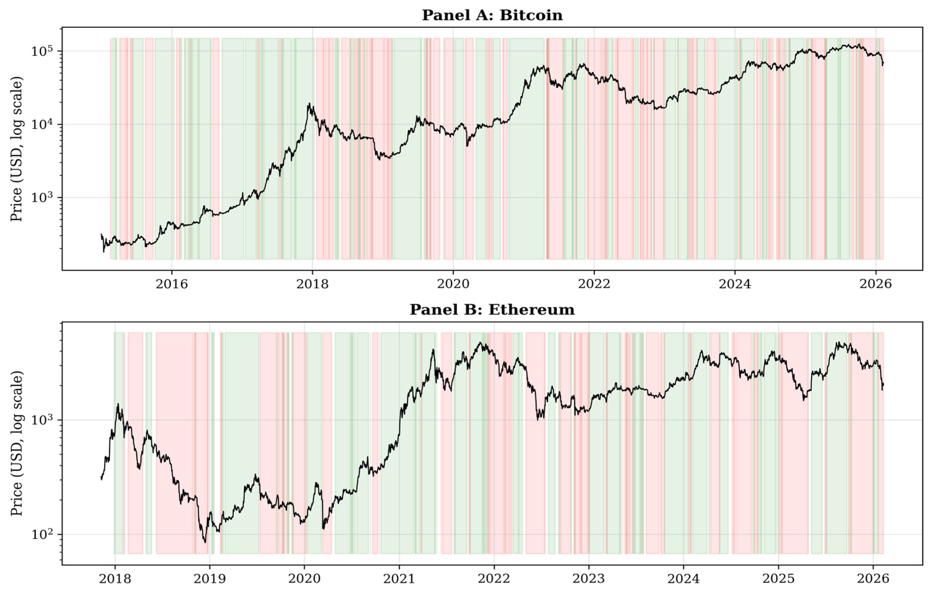
Figure A1. Daily closing prices (log scale) with market state classification. Green shading = Bull state; red shading = Bear state; unshaded = Neutral. Panel (A): Bitcoin (2015–2026). Panel (B): Ethereum (2017–2026). State classification based on 50-day SMA dynamics (see Section 3.1).
Fintech 05 00028 g0a1
Figure A2. 30-day rolling standard deviation (σ) with median-based regime classification. Red = high-uncertainty regime; blue = low-uncertainty regime. Dashed horizontal line = median threshold (BTC: 3.03%; ETH: 4.01%). See Section 3.1.
Fintech 05 00028 g0a2
Table A1. Mann–Whitney U-tests: high- vs. low-volatility regime (complete results).
AssetMetricMW Statp-ValueMean HighMean LowSig.
BTCVaR12,674,845<0.00110.5688.460***
BTCVaR52,656,657<0.0015.8804.484***
BTCCVaR12,412,616<0.00114.26311.617***
BTCCVaR52,648,923<0.0018.9657.124***
BTCMDD2,258,964<0.00154.22544.123***
ETHVaR11,143,808<0.00113.18311.223***
ETHVaR51,222,949<0.0017.3286.177***
ETHCVaR11,168,407<0.00118.26415.109***
ETHCVaR51,215,293<0.00111.2379.483***
ETHMDD1,149,246<0.00169.92359.933***
Note: MW = Mann–Whitney U-test. High/Low = above/below median 30-day rolling σ (see Section 3.1). *** p < 0.01. All tests are significant at p < 0.001.

Appendix B

Replication Code (Condensed)

The full Python 3.11 analysis code (analysis.py, approximately 400 lines) is available in the repository. Key libraries: yfinance (data retrieval), NumPy and Pandas (computation), SciPy (statistical tests), Statsmodels (Newey–West HAC estimation), Matplotlib (visualization). Below, we reproduce the core computational decisions for replicability.
# Key computational decisions (condensed from analysis.py)
# 1. Data: daily log-returns (%) from Yahoo Finance returns = np.log(prices/prices.shift(1)) * 100
# 2. Rolling VaR/CVaR (365-day window = 1 calendar year (crypto trades 24/7)) for i in range(365, n): w = returns[i-365:i] VaR_1pct[i] = -np.percentile(w, 1)
# historical simulation CVaR_1pct[i] = -w[w <= np.percentile(w, 1)].mean() # expected shortfall # MDD: largest peak-to-trough within window cumret = (1 + w/100).cumprod() MDD[i] = ((cumret.cummax() - cumret)/cumret.cummax()).max() * 100
# 3. Trend test: OLS with Newey-West HAC standard errors from statsmodels.regression.linear_model import OLS from statsmodels.tools import add_constant model = OLS(risk_series, add_constant(time_index)).fit(cov_type=‘HAC’, cov_kwds={‘maxlags’: int(N**(1/3))})
# 4. Exceedance correlations [31] theta = np.percentile(np.abs(pooled_returns), quantile) mask_lo = (r_BTC < -theta) & (r_ETH < -theta) mask_hi = (r_BTC > theta) & (r_ETH > theta) rho_minus = np.corrcoef(r_BTC[mask_lo], r_ETH[mask_lo])[0,1] rho_plus = np.corrcoef(r_BTC[mask_hi], r_ETH[mask_hi])[0,1]

Appendix C

This appendix presents the detailed results of the robustness checks and structural diagnostics summarized in Section 4.5.
Table A2. Structural break results: Bitcoin. Breakpoints identified using binary segmentation with L2 cost on weekly aggregated rolling risk series. Change = (last segment mean − first segment mean)/|first segment mean| × 100.
MetricBreak DatesFirst Seg. (%)Last Seg. (%)Change (%)
VaR 1%2017-01, 2019-01, 2023-06−9.64−6.23−35.4
VaR 5%2017-05, 2019-03, 2023-05−3.67−3.69~0
CVaR 1%2020-03, 2021-04, 2023-09−14.28−7.61−46.7
CVaR 5%2017-04, 2019-01, 2023-06−7.45−5.35−28.1
MDD2018-02, 2019-05, 2023-06−32.66−26.42−19.1
Table A3. Structural break results: Ethereum.
MetricBreak DatesFirst Seg. (%)Last seg. (%)Change (%)
VaR 1%2019-12, 2023-06, 2025-03−16.14−9.65−40.2
VaR 5%2019-06, 2023-06, 2024-11−9.59−5.79−39.6
CVaR 1%2020-03, 2022-05, 2023-07−17.68−10.83−38.7
CVaR 5%2019-09, 2023-06, 2025-03−13.21−8.70−34.1
MDD2019-08, 2023-05, 2025-03−88.63−61.32−30.8
Figure A3. Rolling risk measures with structural breakpoints. Blue: daily rolling series. Red dashed: segment means. Red dotted vertical: breakpoint dates. (Left): BTC. (Right): ETH. Rows: VaR 1%, VaR 5%, CVaR 1%, CVaR 5%, Maximum Drawdown.
Fintech 05 00028 g0a3
Figure A4. Rolling Hill tail index (365-day window). Red dashed: linear trend. BTC: trend coef. = +0.000253, t = 3.03, p = 0.002. ETH: trend coef. = +0.000398, t = 3.44, p < 0.001. Higher alpha = thinner tails.
Fintech 05 00028 g0a4
Figure A5. Rolling GARCH(1,1) persistence (alpha + beta). Red dashed: unit persistence (IGARCH). Red solid: linear trend. BTC: trend = −0.000468, p = 0.001. ETH: trend = −0.005697, p = 0.020.
Fintech 05 00028 g0a5
Table A4. Regime-conditional mean VaR 1%: SMA(50) vs. SMA(200).
AssetSMAEarly BullEarly BearLate BullLate Bear
BTCSMA(50)−10.33−11.34−8.07−8.91
BTCSMA(200)−10.25−11.66−7.73−9.36
ETHSMA(50)−14.22−14.72−9.55−9.94
ETHSMA(200)−14.07−15.02−9.23−10.43
Table A5. Block-bootstrap 95% confidence intervals for exceedance correlations (block = 20 days, B = 5000).
PeriodQuantileTailEstimate95% CI Lower95% CI UpperN
Full5%ρ0.6230.3010.8383015
Full5%ρ+−0.124−0.2890.1103015
Full10%ρ0.6300.3830.8123015
Full10%ρ+0.055−0.1080.2483015
Early5%ρ0.7000.2570.8731508
Early5%ρ+−0.278−0.479−0.0001508
Late5%ρ0.6450.3700.7711507
Late5%ρ+0.2770.0940.4091507
Early10%ρ0.6300.2980.8401508
Early10%ρ+−0.099−0.2790.1591508
Late10%ρ0.6960.5220.7861507
Late10%ρ+0.3770.2270.4841507
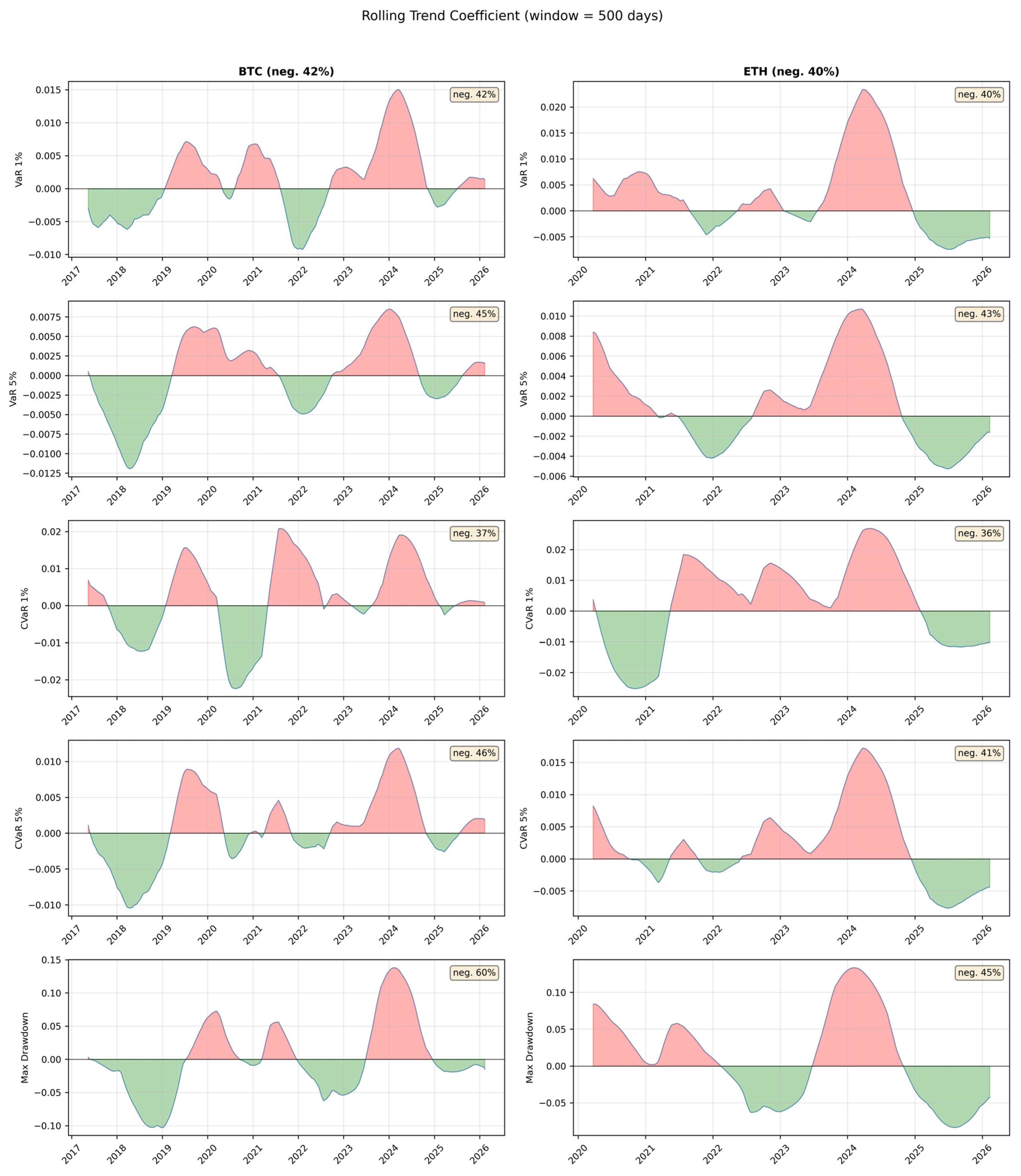
Figure A6. Rolling trend coefficients (500-day window). Green: negative coefficient (declining risk). Red: positive (rising risk). Risk-increasing episodes coincide with known crises (the 2018 Bear market, COVID-19, Terra/FTX).
Fintech 05 00028 g0a6
Table A6. Non-overlapping annual window trend regressions.
AssetMetricN WindowsTrend Coef.R2p-Value
BTCVaR 1%110.5400.4680.020
BTCVaR 5%110.1430.0740.417
BTCMDD111.2510.0500.508
ETHVaR 1%81.3170.7740.004
ETHVaR 5%80.5760.6090.022
ETHMDD83.8030.2530.203

References

  1. Jung, H.S.; Lee, H. Bitcoin research in business and economics: A bibliometric and topic modeling review. FinTech 2025, 4, 68. [Google Scholar] [CrossRef]
  2. Nakamoto, S. Bitcoin: A Peer-to-Peer Electronic Cash System. 2008. Available online: https://bitcoin.org/bitcoin.pdf (accessed on 2 February 2026).
  3. Bongini, P.A.; Mattassoglio, F.; Pedrazzoli, A.; Vismara, S. Crypto ecosystem: Navigating the past, present, and future of decentralized finance. J. Technol. Transf. 2025, 50, 2054–2075. [Google Scholar] [CrossRef]
  4. Bekaert, G.; Harvey, C.R. Foreign speculators and emerging equity markets. J. Financ. 2000, 55, 565–613. [Google Scholar] [CrossRef]
  5. Drożdż, S.; Gębarowski, R.; Minati, L.; Oświęcimka, P.; Wątorek, M. Bitcoin market route to maturity? Evidence from return fluctuations, temporal correlations and multiscaling effects. Chaos 2018, 28, 071101. [Google Scholar] [CrossRef] [PubMed]
  6. Urquhart, A. The inefficiency of Bitcoin. Econ. Lett. 2016, 148, 80–82. [Google Scholar] [CrossRef]
  7. Bariviera, A.F. The inefficiency of Bitcoin revisited: A dynamic approach. Econ. Lett. 2017, 161, 1–4. [Google Scholar] [CrossRef]
  8. Noda, A. On the evolution of cryptocurrency market efficiency. Appl. Econ. Lett. 2021, 28, 433–439. [Google Scholar] [CrossRef]
  9. Mokni, K.; El Montasser, G.; Ajmi, A.N.; Bouri, E. On the efficiency and its drivers in the cryptocurrency market: The case of Bitcoin and Ethereum. Financ. Innov. 2024, 10, 39. [Google Scholar] [CrossRef]
  10. Katsiampa, P. Volatility estimation for Bitcoin: A comparison of GARCH models. Econ. Lett. 2017, 158, 3–6. [Google Scholar] [CrossRef]
  11. Phillip, A.; Chan, J.S.; Peiris, S. A new look at cryptocurrencies. Econ. Lett. 2018, 163, 6–9. [Google Scholar] [CrossRef]
  12. Bouri, E.; Azzi, G.; Dyhrberg, A.H. On the return-volatility relationship in the Bitcoin market around the price crash of 2013. Economics 2017, 11, 2. [Google Scholar] [CrossRef]
  13. Trucíos, C.; Taylor, J.W. A comparison of methods for forecasting Value at Risk and Expected Shortfall of cryptocurrencies. J. Forecast. 2023, 42, 989–1007. [Google Scholar] [CrossRef]
  14. Wu, H.T.; Yueh, M.L. Cryptocurrency risk management using Lévy processes and time-varying volatility. Rev. Quant. Financ. Account. 2026, 66, 33–61. [Google Scholar] [CrossRef]
  15. Malek, J.; Nguyen, D.K.; Sensoy, A.; Tran, Q.V. Modeling dynamic VaR and CVaR of cryptocurrency returns with alpha-stable innovations. Financ. Res. Lett. 2023, 55, 103817. [Google Scholar] [CrossRef]
  16. Subramoney, S.D.; Chinhamu, K.; Chifurira, R. Value at Risk long memory volatility models with heavy-tailed distributions for cryptocurrencies. Front. Appl. Math. Stat. 2025, 11, 1567626. [Google Scholar] [CrossRef]
  17. Katsiampa, P. Volatility co-movement between Bitcoin and Ether. Financ. Res. Lett. 2019, 30, 221–227. [Google Scholar] [CrossRef]
  18. Bouri, E.; Shahzad, S.J.H.; Roubaud, D. Co-explosivity in the cryptocurrency market. Financ. Res. Lett. 2019, 29, 178–183. [Google Scholar] [CrossRef]
  19. Maghyereh, A.; Ziadat, S.A. Pattern and determinants of tail-risk transmission between cryptocurrency markets: New evidence from recent crisis episodes. Financ. Innov. 2024, 10, 77. [Google Scholar] [CrossRef]
  20. Zhu, Y.; Taasim, S.I.; Daud, A. Volatility modeling and tail risk estimation of financial assets: Evidence from gold, oil, bitcoin, and stocks for selected markets. Risks 2025, 13, 138. [Google Scholar] [CrossRef]
  21. Borri, N. Conditional tail-risk in cryptocurrency markets. J. Empir. Financ. 2019, 50, 1–19. [Google Scholar] [CrossRef]
  22. Lo, A.W. The adaptive markets hypothesis: Market efficiency from an evolutionary perspective. J. Portf. Manag. 2004, 30, 15–29. [Google Scholar] [CrossRef]
  23. Aslam, F.; Memon, B.A.; Hunjra, A.I.; Bouri, E. The dynamics of market efficiency of major cryptocurrencies. Glob. Financ. J. 2023, 58, 100899. [Google Scholar] [CrossRef]
  24. Canh, N.P.; Wongchoti, U.; Thanh, S.D.; Thong, N.T. Systematic risk in cryptocurrency market: Evidence from DCC-MGARCH model. Financ. Res. Lett. 2019, 29, 90–100. [Google Scholar] [CrossRef]
  25. Tiwari, A.K.; Adewuyi, A.O.; Albulescu, C.T.; Wohar, M.E. Empirical evidence of extreme dependence and contagion risk between main cryptocurrencies. N. Am. J. Econ. Financ. 2020, 51, 101083. [Google Scholar] [CrossRef]
  26. Bouri, E.; Benbachir, S.; Alaoui, M.E. How do Bitcoin market trends affect major cryptocurrencies? Phys. A Stat. Mech. Its Appl. 2025, 668, 130587. [Google Scholar] [CrossRef]
  27. Ahelegbey, D.F.; Giudici, P.; Mojtahedi, F. Crypto Asset Portfolio Selection. FinTech 2022, 1, 63–71. [Google Scholar] [CrossRef]
  28. Sruthi, S.; Saravanan, D. Forecasting cryptocurrency prices in the DeFi ecosystem using predictive models. In Proceedings of the 2025 International Conference on Computing for Sustainability and Intelligent Future (COMP-SIF), Bangalore, India, 21–22 March 2025; IEEE: New York, NY, USA, 2025; pp. 1–6. [Google Scholar]
  29. Surana, G.; Kaur, H.; Singla, L.; Jain, B.; Ahuja, V. Cryptocurrency Price Prediction Using a Hybrid Deep Learning Approach: Integrating CNN and Random Forest for Enhanced Forecasting. In Proceedings of the 2025 5th International Conference on Intelligent Technologies (CONIT), Huzhou, China, 19–22 September 2025; IEEE: New York, NY, USA, 2025; pp. 1–6. [Google Scholar]
  30. Artzner, P.; Delbaen, F.; Eber, J.-M.; Heath, D. Coherent measures of risk. Math. Financ. 1999, 9, 203–228. [Google Scholar] [CrossRef]
  31. Longin, F.; Solnik, B. Extreme correlation of international equity markets. J. Financ. 2001, 56, 649–676. [Google Scholar] [CrossRef]
  32. Ang, A.; Chen, J. Asymmetric correlations of equity portfolios. J. Financ. Econ. 2002, 63, 443–494. [Google Scholar] [CrossRef]
  33. Truong, C.; Oudre, L.; Vayer, N. Selective review of offline change point detection methods. Signal Process. 2020, 167, 107299. [Google Scholar] [CrossRef]
  34. Caporale, G.M.; Zekokh, T. Modelling volatility of cryptocurrencies using Markov-Switching GARCH models. Res. Int. Bus. Financ. 2019, 48, 143–155. [Google Scholar] [CrossRef]
  35. Liashenko, O.; Adamyk, B.; Adamyk, O. Replication package: BTC–ETH tail risk dynamics and market maturation (365-day rolling windows). Zenodo 2026. [Google Scholar] [CrossRef]
  36. Liashenko, O.; Adamyk, B.; Adamyk, O. Replication package: BTC–ETH tail risk dynamics and market maturation (365-day rolling windows) V2 (Version 2) [Data set]. Zenodo 2026. [Google Scholar] [CrossRef]
Figure 1. 365-day rolling Value-at-Risk (VaR) at 1% and 5% confidence levels. Panel (A): Bitcoin (2016–2026). Panel (B): Ethereum (2018–2026). Shaded area = VaR spread (VaR1% − VaR5%). Dashed black line = linear trend. Both assets exhibit statistically significant declining trends (see Table 4).
Fintech 05 00028 g001
Figure 2. 365-day rolling Conditional Value-at-Risk (CVaR) at 1% and 5% levels. CVaR measures expected loss conditional on exceeding the VaR threshold. Dashed black = linear trend. Note the convergence of BTC and ETH CVaR levels in the later sample period.
Fintech 05 00028 g002
Figure 3. 365-day rolling Maximum Drawdown (MDD). Panel (A): Bitcoin. Panel (B): Ethereum. MDD = largest peak-to-trough decline within each 365-day rolling window.
Fintech 05 00028 g003
Figure 4. Distribution of risk metrics by market state. Top row: Bitcoin. Bottom row: Ethereum. Green = Bull, grey = Neutral, red = Bear. Box = IQR, horizontal line = median, whiskers = 1.5 × IQR. Diamonds indicate outliers.
Fintech 05 00028 g004
Figure 5. Risk metrics by volatility regime and sub-period. (Top): Bitcoin. (Bottom): Ethereum. Red = high-uncertainty regime; blue = low-uncertainty regime. Left bars = early sub-period; right bars = late sub-period. Maturation effects are visibly larger in low-uncertainty regimes.
Fintech 05 00028 g005
Figure 6. BTC–ETH correlation dynamics. Panel (A): the 90-day rolling Pearson (blue) and Spearman (orange) correlations. Dashed horizontal = full-sample Pearson (ρ = 0.792). Green/red shading = BTC Bull/Bear market states. Panel (B): the 365-day rolling exceedance correlations at the 90th percentile. Red = lower tail (ρ); green = upper tail (ρ+). Note the persistent and widening gap between ρ and ρ+.
Fintech 05 00028 g006
Figure 7. BTC–ETH return scatter plots with exceedance zones (90th percentile threshold). (Left panel): early (2018–2020). (Right panel): late (2021–2026). Red quadrant = lower tail (joint extreme losses); green quadrant = upper tail (joint extreme gains). Note the tight clustering of red-zone points vs. the dispersion of green-zone points, particularly in the late period.
Fintech 05 00028 g007
Table 1. Descriptive statistics of daily returns (%).
StatisticBTC Daily ReturnETH Daily Return
Mean0.1330.061
Median0.1210.063
Std Dev3.5494.549
Skewness−0.740−0.780
Excess Kurtosis11.92410.534
Min−46.473−55.073
Max22.51223.474
JB Statistic24,346.2 ***14,193.2 ***
ADF Statistic−65.45 ***−16.52 ***
Observations40583015
Note: Returns are computed as log-returns multiplied by 100. Sample period: BTC 01/01/2015–10/02/2026; ETH 09/11/2017–10/02/2026. JB = Jarque–Bera test for normality; ADF = augmented Dickey–Fuller test for stationarity. *** denotes significance at 1%. Source: Yahoo Finance.
Table 2. Descriptive statistics of daily log-returns (%).
StatisticBTCETH
Mean0.13280.0608
Median0.12050.0631
Std Dev3.54874.5490
Skewness−0.7403−0.7804
Excess Kurtosis11.924110.5336
Min−46.4730−55.0732
Max22.511923.4741
JB Stat24,346.235914,193.2198
JB p-value<0.001<0.001
ADF Stat−65.4507−16.5204
ADF p-value<0.001<0.001
Obs40583015
Note: Returns computed as rt = ln(Pt/Pt−1) × 100. BTC: 02/01/2015–10/02/2026; ETH: 10/11/2017–10/02/2026. JB = Jarque–Bera test. ADF = augmented Dickey–Fuller test (max lag = 20). Source: Yahoo Finance.
Table 3. (a) BTC annual market state distribution and risk characteristics. (b) ETH annual market state distribution and risk characteristics.
(a)
YearP (Bull)P (Bear)P (Neutral)Mean Ret%Vol%Min PriceMax Price
20150.4480.2390.3130.0873.044178465
20160.6640.1530.1830.2202.125364976
20170.8360.0270.1370.7364.40377819,497
20180.1480.6220.230−0.3643.832323717,527
20190.4470.3700.1840.1793.375339913,016
20200.5900.2240.1860.3813.440497129,002
20210.5730.3210.1070.1284.05329,37467,567
20220.1420.6960.162−0.2823.32915,78747,687
20230.6550.2580.0880.2572.20216,62544,167
20240.5630.2190.2190.2172.69839,507106,141
20250.4140.4380.148−0.0182.13276,272124,753
20260.2930.5370.171−0.5883.21562,70296,929
(b)
YearP (Bull)P (Bear)P (Neutral)Mean Ret%Vol%Min PriceMax Price
20180.1510.6930.156−0.4765.228841396
20190.4410.3730.186−0.0083.996105337
20200.6720.1780.1500.4754.701111752
20210.6520.1840.1640.4405.2477304812
20220.1950.6220.184−0.3084.4939943830
20230.5970.2710.1320.1772.36912012379
20240.4970.3440.1580.1043.27522114066
20250.3560.5420.101−0.0323.89514734831
20260.3900.5370.073−0.9524.42818223355
Note: Bull: price > SMA50 and SMA50 rising. Bear: price < SMA50 and SMA50 falling. Neutral: other. Vol% = mean 30-day rolling σ. Source: authors’ calculations. The ETH sample began in November 2017.
Table 4. Linear trend tests for rolling risk metrics (Newey–West HAC standard errors).
AssetMetricβ1 (×104)NW t-Statp-ValueR2NDir.Sig.
BTCVaR1−14.3434−13.7953<0.0010.46793693***
BTCVaR5−4.7335−4.8203<0.0010.11153693***
BTCCVaR1−22.2963−14.9195<0.0010.38183693***
BTCCVaR5−11.1443−10.5319<0.0010.36483693***
BTCMDD−37.5318−3.2977<0.0010.04513693***
ETHVaR1−34.2480−23.4335<0.0010.67452650***
ETHVaR5−14.7335−15.0145<0.0010.51922650***
ETHCVaR1−48.8353−13.1827<0.0010.47642650***
ETHCVaR5−26.0311−19.3515<0.0010.61372650***
ETHMDD−125.9434−9.4588<0.0010.29672650***
Note: Model: Riskt = β0 + β1t + εt. Newey–West HAC SE, bandwidth = N^(1/3). Window = 365 days (crypto markets operate 24/7/365). β1 × 10⁴ for readability. *** p < 0.01, ** p < 0.05, and * p < 0.10. Dir. indicates the direction of the estimated time trend: ↓ = decreasing trend over time; ↑ = increasing trend over time.
Table 5. Risk metrics by market state (mean values).
AssetStateNVaR 1%VaR 5%CVaR 1%CVaR 5%MDDKW p
BTCBear12379.895.7013.078.4755.4<0.001 ***
BTCBull18499.224.8012.817.7145.2
BTCNeutral6079.655.3213.098.2048.8
ETHBear98612.086.7015.7610.1764.60.016
ETHBull126211.996.6116.9910.2563.9
ETHNeutral40212.546.9617.0210.6265.6
Note: Mean values of 365-day rolling metrics. KW = Kruskal–Wallis H-test statistic for VaR 1%. *** indicates statistical significance at the 1% level (p < 0.01). Full Mann–Whitney pairwise tests are reported in Table A1 (Appendix A).
Table 6. Sub-period comparison of tail risk metrics.
AssetMetricEarlyLateΔ (%)MW pSig.Period
BTCVaR110.988.56−22.0<0.001***15–19/20–26
BTCVaR55.814.77−17.9<0.001***15–19/20–26
BTCCVaR114.3212.04−15.9<0.001***15–19/20–26
BTCCVaR59.127.34−19.5<0.001***15–19/20–26
BTCMDD51.5047.66−7.5<0.001***15–19/20–26
ETHVaR114.9010.94−26.6<0.001***17–20/21–26
ETHVaR57.816.23−20.3<0.001***17–20/21–26
ETHCVaR120.7714.75−29.0<0.001***17–20/21–26
ETHCVaR512.399.39−24.3<0.001***17–20/21–26
ETHMDD78.7758.43−25.8<0.001***17–20/21–26
Note: BTC Early = 2015–2019, Late = 2020–2026. ETH Early = 2017–2020, Late = 2021–2026. MW = Mann–Whitney U-test. *** indicates statistical significance at the 1% level (p < 0.01). All p < 0.001.
Table 7. Sub-period comparison by volatility regime (regime × sub-period interaction).
AssetRegimeMetricEarlyLateΔ (%)MW pSig.
BTCHighVaR111.459.77−14.7<0.001***
BTCLowVaR110.257.63−25.6<0.001***
BTCHighCVaR114.7413.83−6.2<0.001***
BTCLowCVaR113.6810.67−22.0<0.001***
BTCHighMDD53.9554.471.00.176
BTCLowMDD47.8342.44−11.3<0.001***
ETHHighVaR115.1412.00−20.7<0.001***
ETHLowVaR114.599.99−31.6<0.001***
ETHHighCVaR121.1016.64−21.1<0.001***
ETHLowCVaR120.3413.08−35.7<0.001***
ETHHighMDD82.0462.94−23.3<0.001***
ETHLowMDD74.4554.42−26.9<0.001***
Note: Interaction of sub-period and volatility regime. BTC MDD in high regime: Δ = +1.0%, p = 0.176 (not significant). *** indicates statistical significance at the 1% level (p < 0.01). All other comparisons are significant at p < 0.001.
Table 8. Exceedance correlations: full sample [31].
Thresholdρ (Lower)ρ+ (Upper)ρ − ρ+N (Lower)N (Upper)
75th0.83060.44400.3866233206
90th0.84680.24640.60048367
95th0.88030.23330.64704430
Note: ρ = Pearson correlation conditional on both returns below − θ. ρ+ = both above + θ. θ = given percentile of pooled absolute returns. N = number of observations satisfying the conditioning criterion.
Table 9. Exceedance correlations by sub-period.
PeriodThresholdρρ+ρ − ρ+N loN up
Early (2018–2020)75th0.87290.48050.39249571
Early (2018–2020)90th0.89450.39750.49703423
Early (2018–2020)95th0.96800.42570.54231711
Late (2021–2026)75th0.78090.38490.3959144134
Late (2021–2026)90th0.75600.08330.67285542
Late (2021–2026)95th0.6218−0.17460.79652420
Note: Early = 2018–2020; late = 2021–2026. Thresholds computed within each sub-period.
Table 10. BTC–ETH correlation by market state.
StateNPearson ρpSpearman ρp
Bull13540.6597<0.0010.7192<0.001
Bear11710.8918<0.0010.8700<0.001
Neutral4900.8002<0.0010.7646<0.001
Note: Market state = BTC 50-day SMA classification. All correlations are significant at p < 0.001.
Disclaimer/Publisher’s Note: The statements, opinions and data contained in all publications are solely those of the individual author(s) and contributor(s) and not of MDPI and/or the editor(s). MDPI and/or the editor(s) disclaim responsibility for any injury to people or property resulting from any ideas, methods, instructions or products referred to in the content.