Article

Offshore Wind Resource Assessment and Wind Farm Optimization Using Machine Learning and CFD Modelling


1
Department of Climate Science and Meteorological Engineering, Istanbul Technical University, Ayazaga, 34469 Istanbul, Türkiye
2
Department of Climate Science and Meteorological Engineering, University of Samsun, 19 Mayis, 55000 Samsun, Türkiye
*
Author to whom correspondence should be addressed.
Submission received: 25 June 2026 / Revised: 31 July 2026 / Accepted: 12 August 2026 / Published: 15 September 2026
(This article belongs to the Special Issue Wind Energy Resource Development and the Sustainable Environment)

Abstract

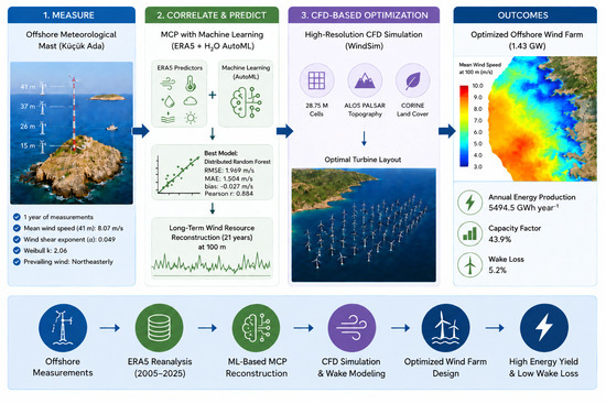
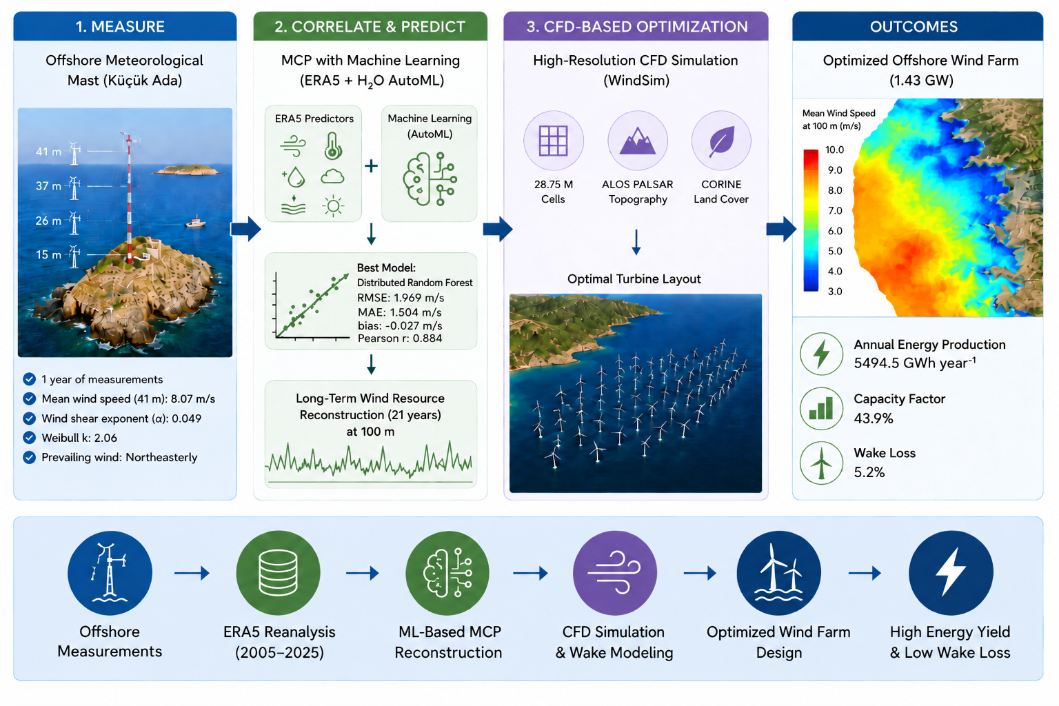
This study presents an integrated framework for offshore wind resource assessment and wind farm micrositing in the Northern Aegean Sea of Türkiye by combining machine learning-assisted measure–correlate–predict (MCP) modelling, long-term reanalysis data and computational fluid dynamics (CFD). One year of measurements from a 41 m meteorological mast on Küçük Ada, offshore Aliağa, İzmir, was analyzed together with a 21-year ECMWF Reanalysis v5 (ERA5) dataset. The measurements indicated a mean annual wind speed of 8.07 m/s, a wind shear exponent of 0.049, a Weibull shape parameter of 2.06 and a persistent northeasterly wind regime. Long-term conditions were reconstructed using 64 meteorological and cyclic predictors derived from four ERA5 grid points and their bilinear interpolation to the mast location. Five H2O algorithm families were evaluated using randomized grid searches and 12-fold temporal cross-validation. Distributed Random Forest provided the best performance for 100 m wind speed, with RMSE = 1.969 m/s, MAE = 1.504 m/s, bias = −0.027 m/s and an out-of-fold Pearson correlation coefficient of r = 0.884. TreeSHAP analysis was applied to interpret predictor contributions. High-resolution WindSim simulations with 28.75 million cells, ALOS PALSAR topography and CORINE land-cover data supported turbine micrositing. The proposed 1.43 GW wind farm yielded 5494.5 GWh/year after wake losses, with a capacity factor of 43.9% and an overall wake loss of 5.2%. The framework provides a robust basis for offshore wind development in Türkiye.

Graphical Abstract

1. Introduction

The transition of the global energy system toward low-carbon and renewable resources has become a fundamental requirement for mitigating climate change, improving energy security and reducing dependence on fossil fuel-based electricity generation [1,2,3]. Within this transformation, wind energy has emerged as one of the most mature and rapidly expanding renewable energy technologies. In recent years, offshore wind energy has gained particular importance because marine environments generally provide stronger, more persistent and less turbulent wind regimes than onshore locations, thereby supporting higher capacity factors and large-scale electricity generation [4,5,6]. According to recent global assessments cited in this study, the worldwide wind power capacity reached approximately 1136 GW by the end of 2024, while offshore wind capacity accounted for nearly 83 GW of this total [7]. These developments indicate that offshore wind energy is no longer a regional renewable energy option, but rather a strategic component of the global decarbonization pathway. The growing importance of offshore wind energy is closely related to the increasing demand for high-capacity renewable energy systems. Global energy-transition scenarios emphasize the central role of large-scale, low-cost renewable electricity systems in achieving a sustainable and low-carbon energy supply [8,9]. Offshore wind farms are particularly suitable for this purpose due to the availability of large marine areas, reduced surface roughness, higher average wind speeds and improved turbine performance under offshore atmospheric conditions [10,11]. In addition, the continuous increase in offshore turbine size, hub height and rotor diameter has significantly improved the technical feasibility and energy yield performance of offshore projects [12,13]. Therefore, offshore wind energy has become an essential technology for supporting long-term carbon neutrality targets, especially in countries with extensive coastlines and favorable marine wind regimes.
Türkiye faces similar challenges in its national energy transition. Although the share of renewable energy in Türkiye’s installed power capacity has increased substantially in recent years, electricity generation still remains significantly associated with fossil fuel resources, particularly natural gas and imported coal [14]. This structure creates important challenges in terms of greenhouse gas emissions, energy import dependency, electricity supply security and economic vulnerability. Türkiye’s long-term climate policy framework, including its 2053 net-zero emission target, requires a strong increase in renewable electricity generation and a gradual reduction in the carbon intensity of the energy sector [15,16]. In this context, offshore wind energy represents a strategic renewable energy option for Türkiye because of the country’s long coastlines, favorable regional wind climatology, proximity of potential offshore wind areas to industrial demand centers, and the possibility of developing large-scale projects beyond the spatial limitations of onshore wind farms.
National and international assessments indicate that Türkiye has considerable offshore wind energy potential. The World Bank offshore wind roadmap for Türkiye identifies an approximate technical offshore wind potential of 75 GW and highlights the Marmara, Aegean and Black Sea regions as promising areas for future offshore wind development [17]. Among these regions, the Northern Aegean Sea is particularly important because of its persistent northerly and northeasterly wind regimes, favorable wind speed characteristics and proximity to industrial and port infrastructure. In addition, the Aegean Sea has been examined in previous wind resource studies using satellite-based and reanalysis approaches, which have emphasized its favorable offshore wind conditions [18,19]. These characteristics indicate that the Northern Aegean offshore region may play an important role in Türkiye’s future offshore wind energy planning.
The academic literature on offshore wind energy in Türkiye has expanded in recent years. Early studies evaluated the offshore wind power potential of Türkiye and identified promising coastal and island regions for future project development [20]. Subsequent studies applied multi-criteria site selection methods and GIS-based spatial analyses to determine suitable offshore wind farm areas in Türkiye’s seas [21,22]. Other studies focused on techno-economic feasibility, regional suitability, or specific project areas such as the Southern Marmara region, Bandırma Bay, Sinop, the Gulf of Edremit, Antakya Gulf, Çanakkale, Bozcaada, Gökçeada and the North Aegean region [23,24,25,26,27,28,29]. These studies have provided valuable contributions to the preliminary understanding of Türkiye’s offshore wind potential and have demonstrated that several coastal and marine regions of the country may be technically suitable for offshore wind development.
However, the existing literature on offshore wind energy in Türkiye is still largely based on reanalysis datasets, satellite-derived products, coastal meteorological stations, land-based measurements, GIS-based suitability analyses and multi-criteria decision-making frameworks [30,31]. Although these approaches are highly useful for regional screening and strategic planning, they may not fully represent the local offshore wind regime, marine atmospheric boundary-layer characteristics, coastal transition effects and site-specific wind variability required for engineering-scale wind farm design. The existing literature indicates that studies based on direct offshore wind measurements remain extremely limited in Türkiye. Furthermore, comprehensive offshore wind farm assessments integrating field observations, long-term wind climate reconstruction, CFD-based microscale flow modelling, wake effect evaluation and energy production analysis within a unified framework are still scarce [32,33,34]. This represents a critical methodological gap for Türkiye’s offshore wind energy development. Reliable offshore wind farm planning requires the integration of short-term site measurements with long-term atmospheric datasets. Reanalysis products such as ERA5 provide spatially and temporally consistent meteorological information over multi-decadal periods and are widely used in wind resource assessment studies [19]. Nevertheless, the relatively coarse spatial resolution of reanalysis datasets may limit their ability to represent local acceleration zones, coastal transition effects, surface roughness contrasts and microscale flow variability. Therefore, MCP approaches are commonly used to reconstruct long-term wind characteristics from short-term measurement campaigns [35]. Recent studies have shown that machine-learning-based MCP and wind reconstruction methods can represent nonlinear relationships between reanalysis predictors and site-specific wind conditions more effectively than conventional regression-based or MCP-corrected reanalysis approaches, thereby improving wind speed reconstruction performance [36,37].
In addition to long-term wind reconstruction, CFD-based microscale modelling is an essential tool for offshore wind farm design and optimization. CFD models allow the detailed representation of terrain-induced flow modification, coastal transition effects, turbulence behavior, spatial wind speed variability and wake interactions between turbines. For large-scale offshore wind farms, wake-aware turbine placement is particularly important because turbine spacing, dominant wind direction and internal flow shadowing directly affect net annual energy production, capacity factor and project efficiency [38,39]. Therefore, the combined use of offshore measurements, long-term reanalysis datasets, machine learning-based MCP modelling and CFD-supported micrositing provides a robust methodological framework for offshore wind resource assessment and wind farm optimization [40,41].
Against this background, this study presents an integrated offshore wind resource assessment and wind farm optimization framework for the Northern Aegean Sea offshore region of Türkiye. The study uses one year of on-site wind measurements obtained from a 41 m meteorological mast installed on Küçük Ada, located offshore of Aliağa, İzmir. These measurements are combined with long-term ERA5 reanalysis data, machine learning-based MCP modelling and CFD simulations performed using WindSim. The methodological framework includes statistical analysis of the measured offshore wind regime, long-term wind reconstruction using multiple ERA5 grid points and atmospheric predictors, microscale CFD-based wind flow simulation, turbine layout assessment, wake-loss evaluation and annual energy production estimation.
This study bridges the gap between offshore field measurements, long-term wind climate reconstruction, machine learning-based MCP modelling, CFD-driven micrositing and utility-scale offshore wind farm assessment within a unified framework. To the authors’ knowledge, this study represents one of the first comprehensive offshore wind energy assessments in Türkiye based on direct offshore on-site wind measurements. In this respect, the study addresses an important data and methodology gap in Türkiye’s offshore wind literature and provides a scientifically grounded engineering framework for future offshore wind energy planning, investment assessment and renewable energy policy development.
The main objectives of this study are therefore: (i) to characterize the offshore wind regime of the Northern Aegean study area using direct on-site measurements; (ii) to reconstruct the long-term offshore wind climate using ERA5 reanalysis data and machine learning-based MCP techniques; (iii) to simulate microscale offshore wind flow patterns using CFD modelling; (iv) to evaluate the energy production potential, wake-loss behavior and capacity factor performance of a large-scale offshore wind farm configuration. By integrating offshore measurements, machine learning-based wind climate reconstruction, CFD modelling and wind farm energy assessment within a unified framework, this study contributes to the scientific and technical foundation for future offshore wind development in Türkiye.

2. Materials and Methods

2.1. Study Area and Wind Measurement Campaign

The study area is located offshore of the Aliağa district in the Northern Aegean region of Türkiye, where offshore wind conditions are characterized by persistent northeasterly to northerly Etesian-related flow regimes and relatively high annual wind speeds [42]. The offshore measurement campaign was conducted using a fixed meteorological mast installed on Küçük Ada, close to the coastal transition zone, to directly represent the marine wind regime of the project area. The measurement campaign covered a one-year period from 30 March 2024 at 00:00 to 30 March 2025 at 00:00. The offshore meteorological mast was located at 38.8630° N latitude and 26.8811° E longitude. All timestamps were recorded in Coordinated Universal Time (UTC + 00:00) and the measurements were stored as 10 min averages. The wind measurement sensors were supported by valid calibration certificates issued by Deutsche WindGuard Wind Tunnel Services GmbH (Varel, Germany), an IECRE- and MEASNET-approved test laboratory accredited by the German Accreditation Body (DAkkS; Berlin, Germany), thereby ensuring documented measurement traceability and compliance with internationally recognized calibration procedures. The measurement system achieved an overall data availability of 95.25%, providing a reliable observational basis for offshore wind resource assessment. Missing data in the in situ time series were handled using a strict quality-control approach. A complete 10 min UTC timestamp sequence was used as reference and only valid measurements were included in the analysis. Missing or invalid records were excluded without interpolation or gap filling to preserve the natural variability of the wind field. Accordingly, all statistical analyses and MCP modelling were performed using only concurrent valid observations from the relevant sensors and ERA5 data. The geographical location of the study area, the position of the offshore meteorological mast on Küçük Ada and the surrounding topographic characteristics are illustrated in Figure 1. The detailed statistical outcomes derived from the in situ measurement campaign are presented in Section 3.1.
These characteristics indicate favorable offshore wind conditions for large-scale energy production and provide an advantageous basis for turbine layout optimization and wake-interaction assessment.
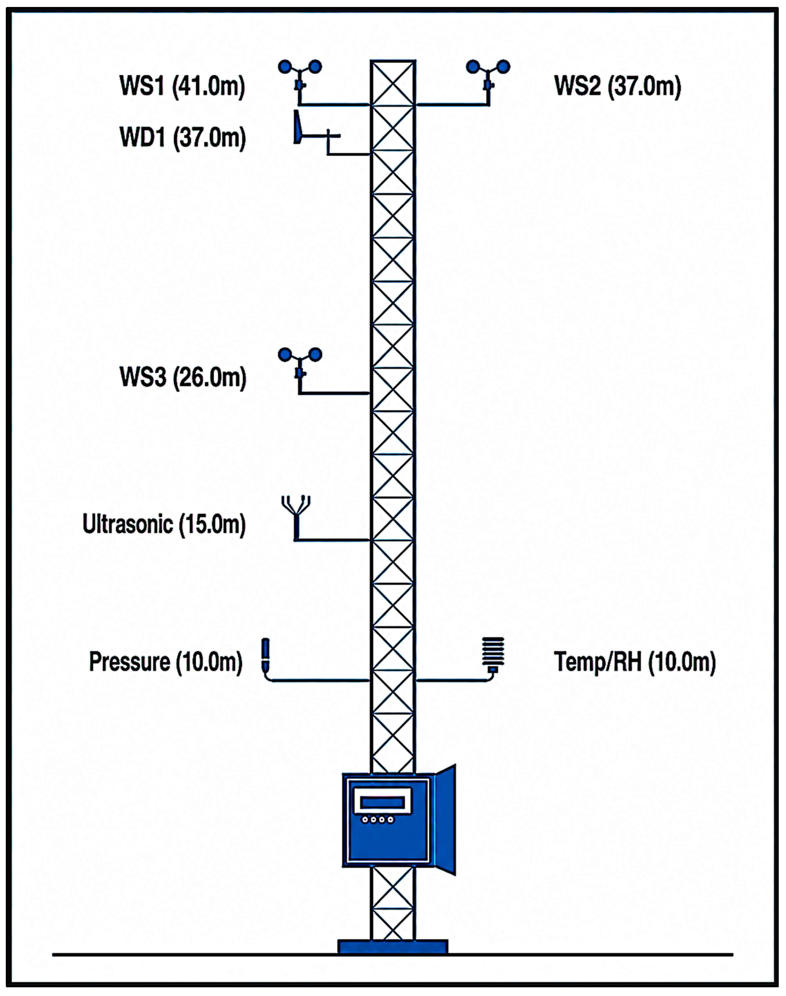
The measurement campaign was designed to characterize the offshore atmospheric boundary layer and to provide reliable meteorological input data for long-term wind reconstruction, machine learning-based MCP modelling and CFD-supported wind farm optimization analyses. The measurement mast included multiple wind speed sensors positioned at different elevations together with wind direction sensors and auxiliary atmospheric instrumentation. This multi-level measurement configuration enabled the assessment of vertical wind speed variation, wind shear behavior and directional consistency under offshore atmospheric conditions. A summary of the measurement system, including sensor specifications, measurement heights, recorded parameters and data recovery rates, is presented in Table 1. The use of calibrated measurement devices with high temporal continuity and a data availability ratio exceeding 95% provided a robust observational basis for offshore wind resource assessment and engineering-scale energy production analyses.
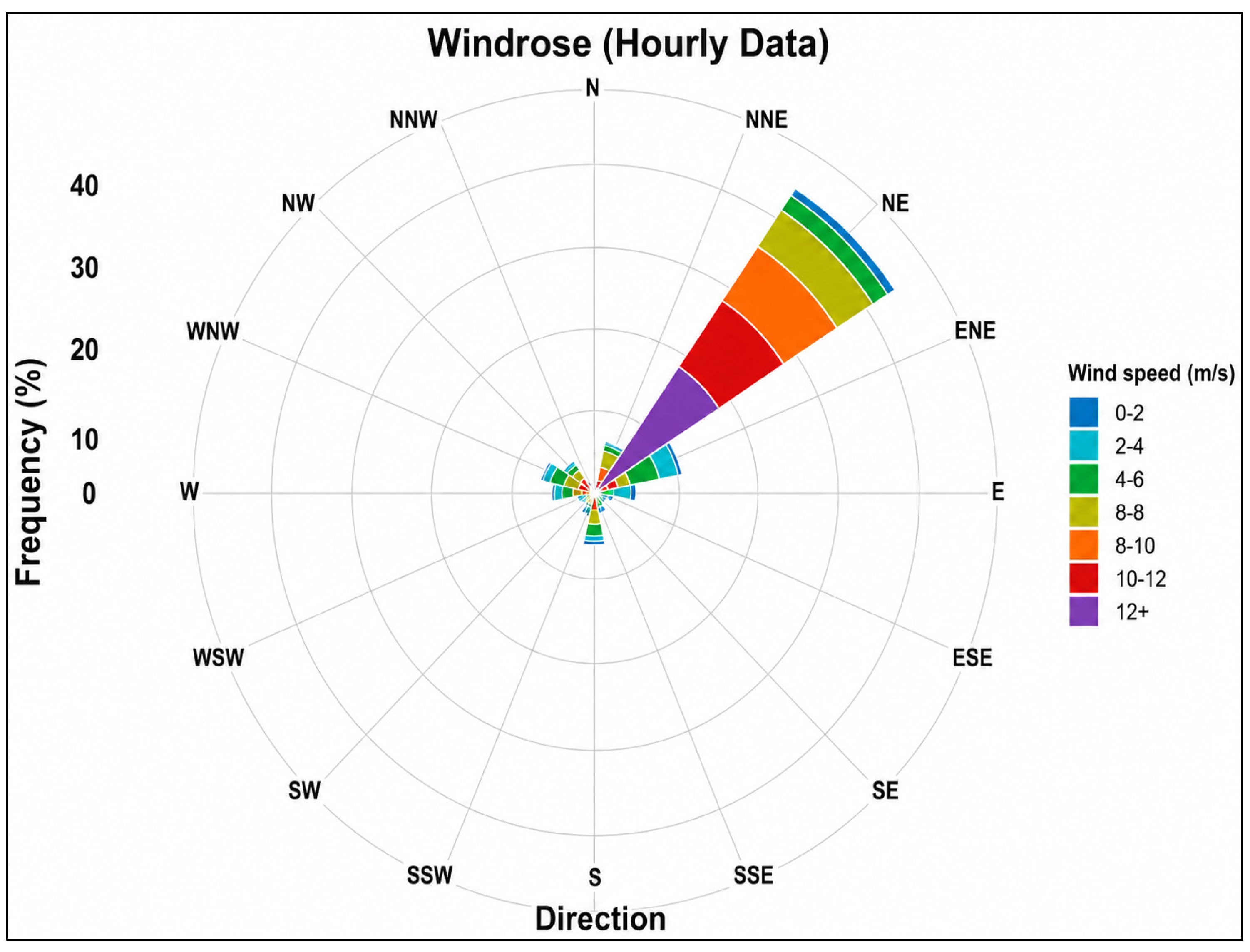
Wind roses derived from the in situ measurements were constructed using concurrent 10 min records of wind speed and wind direction. Because the highest wind speed sensor was installed at 41 m, while the nearest and highest wind direction sensor was installed at 37 m, the on-site wind roses were generated by pairing the 41 m wind speed measurements (WS1) with the concurrent 37 m wind direction measurements (WD1). Only time steps with valid records from both sensors were retained. Missing or invalid wind speed or wind direction values were excluded, and no interpolation or synthetic replacement was applied. Wind directions were grouped into directional sectors, while wind speeds were classified using consistent wind-speed bins. The lowest bin represents calm or near-calm conditions, and the radial axis of each wind rose represents the frequency of occurrence, not wind speed magnitude.

2.2. ERA5 Reanalysis Data and Long-Term Wind Characterization

Long-term atmospheric conditions were represented using the ERA5 reanalysis dataset produced by the European Centre for Medium-Range Weather Forecasts (ECMWF) within the Copernicus Climate Change Service framework. The ERA5 dataset used in this study covers a 21-year period from 2005 to 2025. ERA5 provides hourly atmospheric variables with an approximate horizontal resolution of 0.25° × 0.25°, enabling long-term offshore wind characterization over large spatial domains [19,43,44].
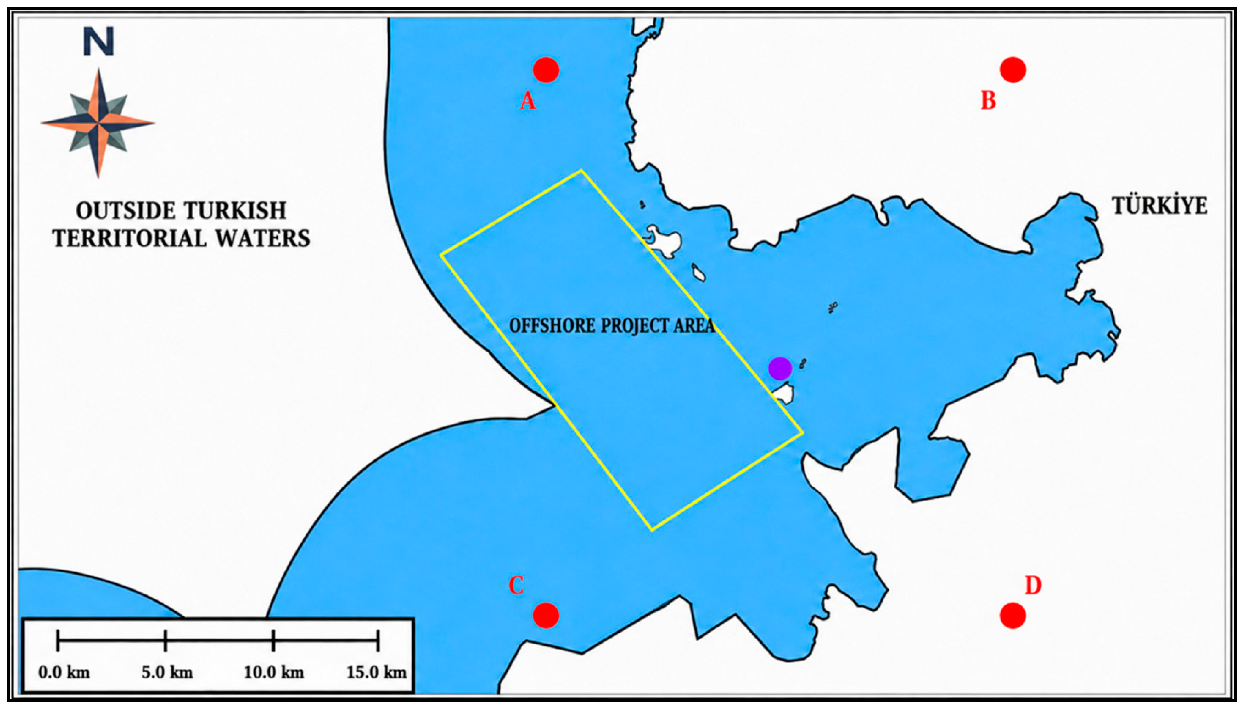
Figure 2 shows the locations of the four ERA5 grid points (A, B, C and D) selected around the offshore meteorological mast. The reference points were positioned at (39.00° N, 26.75° E), (39.00° N, 27.00° E), (38.75° N, 26.75° E) and (38.75° N, 27.00° E), corresponding to distances of 19.0, 18.3, 16.9 and 16.2 km from the measurement site, respectively. Figure 2 provides a schematic spatial overview of the study region, including the offshore meteorological mast location, the four surrounding ERA5 grid points and the candidate offshore wind farm area. In this figure, the blue-shaded marine zone represents Turkish territorial waters, while the unshaded western marine area corresponds to adjacent non-Turkish maritime space. The red circle denotes the in situ mast location, the A–D markers indicate the ERA5 grid points and the yellow-shaded zone represents the potential offshore wind farm area evaluated in this study.
The use of multiple surrounding ERA5 grid points was intended to better capture the spatial variability of atmospheric conditions within the study area, provide a more representative characterization of offshore atmospheric conditions and reduce potential uncertainties associated with relying on a single reanalysis grid cell. The ERA5 datasets extracted for the selected grid points contained a comprehensive set of atmospheric variables describing both surface and upper-air conditions. In addition to near-surface wind, temperature, pressure and boundary-layer parameters, the datasets included thermodynamic and dynamic variables from multiple pressure levels, such as wind components, temperature and geopotential height. The availability of these complementary atmospheric predictors enabled a more detailed representation of offshore atmospheric processes and provided a physically meaningful input dataset for the machine learning-based wind climate reconstruction framework. A summary of the ERA5 variables considered in this study is presented in Table 2.
In order to improve the representation of local offshore atmospheric variability, four ERA5 grid points surrounding the measurement mast were selected and analyzed simultaneously. The dataset included 100 m and 10 m wind components together with additional atmospheric variables such as 2 m temperature, relative humidity, boundary-layer height, surface pressure and surface solar radiation downwards. Relative humidity (%) was derived from 2 m temperature and 2 m dew-point temperature. These parameters were used both for long-term wind characterization and as input variables within the machine learning-based MCP framework.
Comparative analyses between ERA5 outputs and offshore measurements indicated that ERA5 successfully represented the dominant wind direction and general directional frequency characteristics of the study area. However, the reanalysis dataset produced relatively smoother wind speed distributions at higher speed classes due to its gridded structure and inability to fully resolve local offshore acceleration effects and microscale roughness transitions [45,46].

2.3. Machine Learning-Based MCP Modelling

A response-specific machine-learning-assisted measure–correlate–predict (ML-MCP) framework was developed to reconstruct the long-term offshore wind regime from the short-term on-site measurements. Wind speeds measured at 41 m were first extrapolated to 100 m using the power law with the site-specific wind shear exponent α = 0.049, and the resulting 100 m wind-speed series was used as the scalar observational response (ws100_obs). The corresponding corrected wind-direction series was combined with wind speed to derive the zonal and meridional observational responses (u100_obs and v100_obs), while the reconstructed 21-year wind-speed series was subsequently extrapolated from 100 m to the 170 m turbine hub height using the same exponent. The power-law method remains a widely applied engineering approach for hub-height extrapolation when a site-specific shear exponent is available [47].
In the present study, α = 0.049 was derived from concurrent multi-level offshore measurements and represents a site-specific annual mean value rather than a generic offshore assumption. Its relatively low magnitude is physically consistent with the low aerodynamic roughness and weak mean vertical wind-speed gradients generally observed over open-water environments [48], and it results in an approximately 7.2% increase in wind speed between 41 m and 170 m. Nevertheless, a constant annual exponent cannot fully represent stability-dependent, seasonal, diurnal, or synoptic variations in the offshore wind profile; therefore, the reconstructed hub-height wind climate should be interpreted as an annual representative engineering estimate, while stability-resolved or rotor-equivalent approaches would be preferable for detailed transient-flow and rotor-layer analyses [49].
ERA5 predictors were constructed from the four surrounding 0.25° grid points A, B, C and D and from a mast-representative point I obtained through bilinear interpolation, thereby reducing the spatial mismatch between the relatively coarse ERA5 grid and the offshore measurement location [50]. At each of these five spatial representations, the predictor set included 100 m wind speed, 100 m u and v components, 10 m wind speed, 10 m u and v components, surface pressure, boundary-layer height, surface solar radiation downwards, 2 m temperature, derived 2 m relative humidity and derived moist-air density. Four cyclic temporal predictors representing the sine and cosine of hour of day and day of year were also included, resulting in a common matrix of 64 numerical predictors for each response. Wind-speed magnitude was modelled directly in scalar form, whereas wind direction was reconstructed from separately predicted u and v components; this component-based treatment avoids the discontinuity at 0°/360° associated with direct angular regression and follows established MCP practice [51].
The use of atmospheric predictors from multiple surrounding grid points is also consistent with previous multi-grid machine-learning applications in which neighbouring numerical-weather-model outputs improved local wind prediction performance [52]. Model development was performed using controlled, algorithm-specific randomized grid searches implemented with H2O version 3.44.0.3 rather than through the automated H2O AutoML routine. Although AutoML environments provide structured tools for comparing heterogeneous machine-learning algorithms [53], the present study used predefined and controlled randomized searches for Distributed Random Forest (DRF), Gradient Boosting Machine (GBM), XGBoost, Generalized Linear Model (GLM) and Deep Learning. Previous wind-energy studies have similarly demonstrated the effectiveness of combining numerical-weather-prediction variables and feature-selection procedures with boosting-based machine-learning algorithms [54].
Conventional linear regression, variance-ratio MCP and sector-wise linear regression were included as benchmark approaches where applicable [35]. The DRF search considered tree budgets of 300, 500, 700, 900 and 1200; maximum depths of 20, 30, 40 and 50; minimum row sizes of 2, 3, 5 and 10; sampling rates of 0.70, 0.85 and 1.00; and mtries values of −1, 20, 40 and 60. The GBM and XGBoost searches varied tree number and depth, learning rate, minimum row size and row and column sampling; GLM varied alpha and lambda; and Deep Learning varied hidden-layer architecture, input dropout, L1/L2 regularization and learning rate. Across the three response variables, 101 H2O configurations completed training, comprising 33 configurations for ws100_obs and 34 configurations each for u100_obs and v100_obs. Training and validation followed a 12-fold calendar-month-based temporal cross-validation design using month of year as the fold column, in which each monthly fold was excluded from model fitting and used to produce held-out out-of-fold predictions. Records without a valid observational response were not interpolated or gap-filled and were excluded from model calibration and validation. Randomized searches used a fixed seed of 20,260,227 and RMSE-based early stopping with three stopping rounds and a tolerance of 1 × 10⁻⁴. RMSE was used as the primary model-selection criterion, while MAE, bias and Pearson’s correlation coefficient r were used as complementary performance measures; reconstructed wind direction was evaluated using circular RMSE, circular MAE and circular bias.
DRF yielded the lowest out-of-fold RMSE for all three responses and was therefore selected for long-term reconstruction. RMSE-based early stopping retained 168, 166 and 171 effective trees for ws100_obs, u100_obs and v100_obs, respectively, and all three selected models used a maximum depth of 30, a minimum row size of 5, a sampling rate of 0.70 and mtries = 20. The selected scalar model produced the long-term 100 m wind-speed magnitude, whereas the predicted u and v components were combined using the meteorological atan2 convention to reconstruct the corresponding 100 m wind direction. Finally, TreeSHAP contributions were calculated for the three selected DRF models over the concurrent measurement–ERA5 period, and global predictor importance was quantified using the mean absolute SHAP contribution of each variable [55]. The response-specific model architecture, selected DRF ensemble sizes and reconstructed outputs are summarized in Table 3.
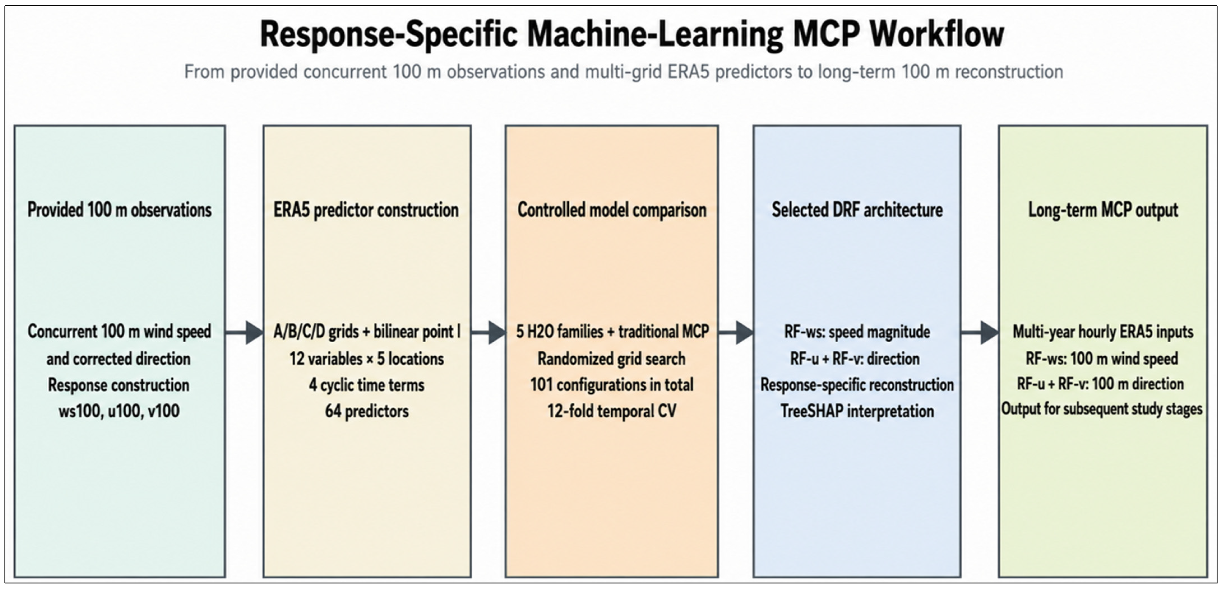
All three responses used the common 64-feature ERA5 predictor matrix. The selected DRF models used a maximum depth of 30, a minimum row size of 5, a sampling rate of 0.70 and mtries = 20. The overall response-specific ML-MCP workflow is illustrated in Figure 3.

2.4. CFD Modelling and Wind Flow Simulation

Microscale wind flow simulations were performed using WindSim 12.0, a CFD-based wind resource assessment platform widely applied in wind energy studies. WindSim solves the steady Reynolds-Averaged Navier–Stokes (RANS) equations and employs two-equation turbulence-closure models to represent atmospheric boundary-layer flow over complex terrain and coastal environments [56].
The computational domain was developed from a high-resolution Advanced Land Observing Satellite Phased Array type L-band Synthetic Aperture Radar (ALOS PALSAR) digital elevation model with a spatial resolution of 12.5 m, while surface roughness characterization was based on the Coordination of Information on the Environment (CORINE) Land Cover dataset. Covering approximately 43.5 km × 44.4 km, the domain included both offshore and surrounding onshore areas to capture mesoscale-to-microscale flow interactions. The model was defined within the Universal Transverse Mercator (UTM) Zone 35 coordinate reference system using the World Geodetic System 1984 (WGS84) datum, with terrain elevations exceeding 1000 m.
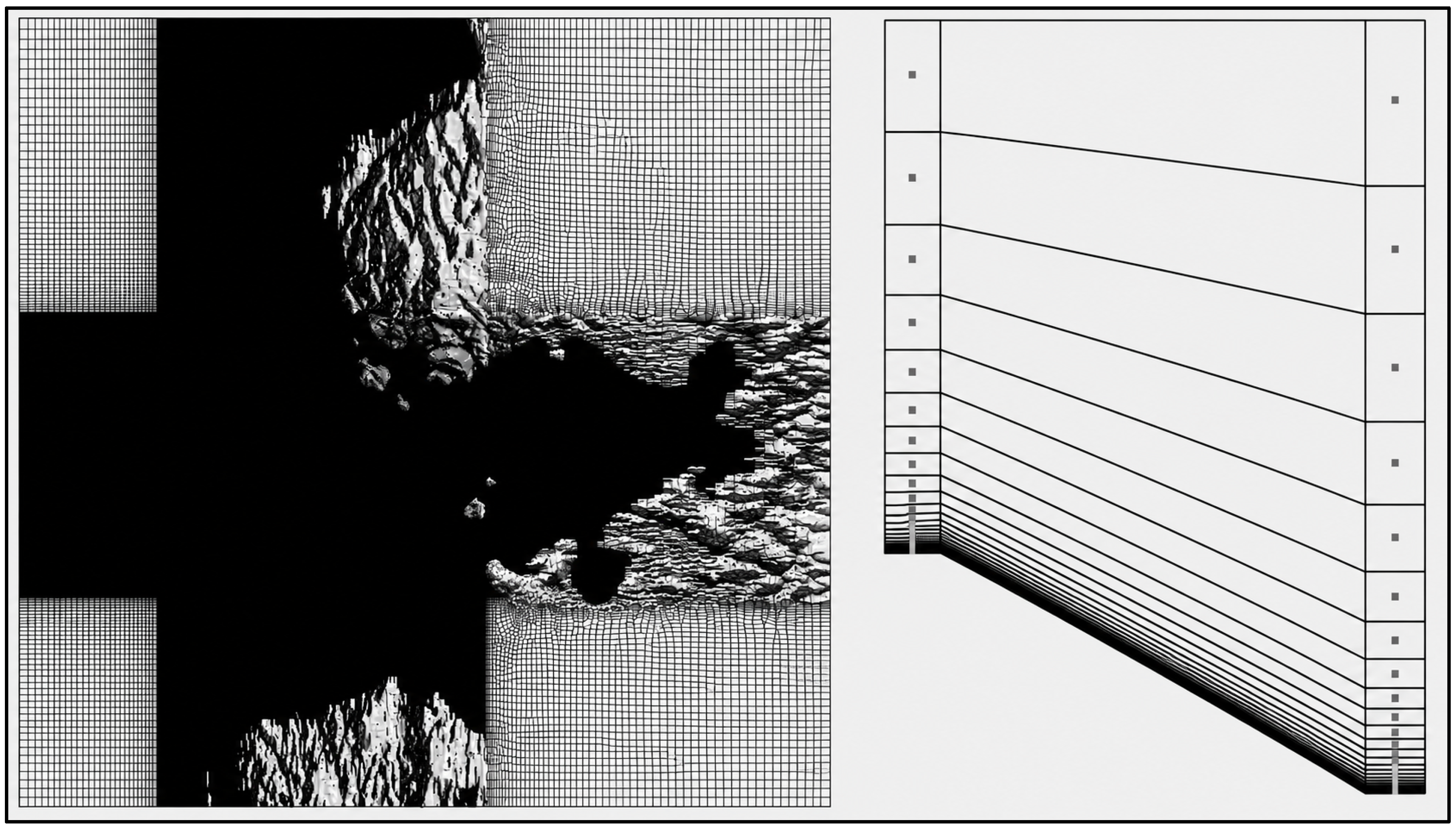
A variable-resolution three-dimensional mesh was generated, with refinement zones applied over the offshore wind farm area and around turbine locations to improve the representation of wind speed gradients, turbulence and wake-related effects. The final CFD grid comprised 995 × 903 horizontal cells and 32 vertical layers, corresponding to approximately 28.75 million computational cells. Horizontal grid spacing ranged from 20.0 to 603.2 m, while near-surface vertical resolution was enhanced with the first nodes located between 1 and 19 m above ground level. Figure 4 illustrates the computational mesh structure used in the CFD simulations, including the horizontal mesh distribution across the study area and the vertical grid configuration. The mesh was progressively refined within the wind farm region and areas of complex terrain to improve the representation of local flow acceleration, turbulence development and terrain-induced wind field variability. The vertical grid structure was designed with a higher node density near the surface, where wind speed gradients and turbulence effects are most pronounced, thereby increasing the accuracy of atmospheric boundary-layer representation.
To generate the numerical wind database, separate CFD simulations were conducted for 12 directional sectors at 30° intervals. The CFD simulations were performed in WindSim 12.0 (WindSim AS, Tønsberg, Norway), with the standard turbulence model and the GCV solver. A boundary-layer height of 500 m, an inflow wind profile normalized to a reference wind speed of 10 m/s at the top of the boundary layer (as specified in the WindSim CFD setup), a fixed-pressure upper boundary condition and a maximum of 5000 iterations were specified, while potential-temperature effects were not activated. Numerical convergence was assessed by monitoring the residual and spot values of the three velocity components (U, V, W), turbulent kinetic energy (k) and turbulence dissipation rate (ε). In accordance with the WindSim convergence procedure, a solution was considered converged when the monitored spot values became stable and the residuals fell below the prescribed convergence threshold [57,58]. All 12 directional sectors satisfied WindSim’s internal convergence criterion after 739–1425 iterations.
The resulting CFD-derived wind atlas was coupled with long-term climatological data to spatially transfer wind characteristics across the study area, estimate hub-height wind conditions, evaluate turbine-to-turbine flow variability and support offshore wind farm layout optimization and energy production assessments.

2.5. Wind Farm Layout and Energy Production Analysis

The offshore wind farm configuration consisted of 65 International Energy Agency (IEA) 22 MW Reference Wind Turbines (IEA-22-280-RWT), each with a hub height of 170 m, resulting in a total installed capacity of 1430 MW [59]. The IEA-22-280-RWT was selected as a next-generation offshore reference turbine rather than as a site-specific commercial procurement option. This reference turbine provides an openly documented and reproducible design basis, including a rated power of 22 MW, a rotor diameter of 284 m, a hub height of 170 m and associated aerodynamic and turbine-model data required for wind farm energy and wake assessment [59]. Such open-reference turbine models are particularly useful in research applications because they enable transparent comparison of wind farm layouts, wake effects and annual energy production estimates without relying on proprietary manufacturer data.
The use of a 22 MW-class turbine is also consistent with the ongoing upscaling trend in offshore wind technology. Recent industrial developments, such as the installation of a 26 MW offshore wind turbine by Dongfang Electric, indicate that very large offshore turbines are becoming technically realistic for future utility-scale offshore wind projects [60]. However, unlike open-reference turbines, detailed commercial power curves, thrust-coefficient curves, controller characteristics and load data for such machines are generally not publicly available. Therefore, the IEA-22-280-RWT was used in this study as a transparent benchmark turbine for scenario-based energy assessment.
It should be noted that the IEA-22-280-RWT is defined as an IEC Class I-B reference turbine. This classification indicates that the turbine is designed for relatively severe wind and turbulence conditions and should not be interpreted as a requirement that the site’s annual mean wind speed must be 10 m/s. The measured annual mean wind speed of 8.07 m/s in this study refers to the 41 m measurement level, whereas the wind farm energy assessment was based on the reconstructed long-term wind climate extrapolated to the 170 m turbine hub height and evaluated through the turbine power curve. Therefore, the selected turbine was used to assess the energy potential of a future large-scale offshore wind farm under the reconstructed hub-height wind distribution. Nevertheless, the use of a Class I-B reference turbine may represent a conservative and not necessarily site-optimized turbine choice; final project development would require detailed site-specific turbine-class selection, load assessment, commercial turbine availability and techno-economic optimization.
Türkiye’s legally applied territorial-sea breadth in the Aegean Sea is 6 nautical miles (approximately 11.1 km). Therefore, the territorial-sea boundary was treated as a mandatory spatial constraint during turbine micrositing and all turbine locations were required to remain within Türkiye’s territorial waters. The final geographic coordinates of all 65 turbine locations are provided in Appendix A. Turbine placement and wake-interaction analyses were performed using the CFD-derived offshore wind atlas together with the dominant offshore wind direction characteristics identified during the measurement analyses. Wake losses were estimated using WindSim Wake Model 3, an analytical engineering wake model based on the formulation developed by Ishihara et al. The model calculates normalized single-wake velocity deficits over the CFD-derived ambient wind field and represents wake expansion as a function of the turbine thrust coefficient, ambient turbulence intensity and wake-generated turbulence. Unlike fully coupled actuator-disc CFD simulations, wake effects are evaluated through a computationally efficient post-processing procedure applied to the ambient flow field [61]. WindSim Wake Model 3 was selected because the Ishihara formulation explicitly accounts for the influence of ambient turbulence intensity and turbine thrust coefficient on wake expansion, velocity recovery and added turbulence. This capability is particularly important for offshore wind farms, where relatively low ambient turbulence levels can lead to slower wake recovery and stronger wake interactions between downstream turbines. The Ishihara–Qian wake formulation was evaluated against large-eddy simulation and wind-tunnel data for model-scale and utility-scale turbines [61]. In addition, operational wind-farm studies have demonstrated the importance of wake-model selection, ambient turbulence intensity and atmospheric stability in estimating farm-level power deficits [62,63]. WindSim Wake Model 3 was selected instead of Jensen, FLORIS, or FUGA because it is directly integrated with the CFD-derived ambient wind field used in this study and accounts for thrust coefficient and ambient turbulence intensity in wake expansion and recovery [61]. Jensen is comparatively simpler, while FLORIS and FUGA require separate modelling frameworks and additional configuration beyond the present WindSim-based workflow. However, WindSim Wake Model 3 remains an analytical post-processing model and does not resolve transient stability effects or fully unsteady three-dimensional wake dynamics. Therefore, the reported wake losses should be interpreted as engineering-scale estimates within the assumptions of the selected model [62,63]. Recent studies have demonstrated that machine-learning-based optimization methods and CFD-supported flow simulations can provide effective tools for improving wind farm layouts and evaluating turbine-to-turbine aerodynamic interactions [64,65]. In the present study, the long-term offshore wind conditions reconstructed through the machine learning-assisted MCP framework were subsequently integrated with the CFD-derived wind atlas to estimate the annual energy production characteristics of the proposed offshore wind farm. Gross and wake-adjusted annual energy production values, wake losses, full-load operating hours and capacity factor values were calculated to evaluate the technical performance of the wind farm configuration.
Wake-interaction analyses demonstrated that turbines located along the dominant wind direction axis experienced relatively stronger flow shadowing effects within the inner sections of the wind farm layout. These analyses were used to evaluate the effectiveness of the proposed turbine arrangement and its influence on gross energy production performance.

3. Results

3.1. Wind Measurement Analysis

The offshore wind measurement analysis demonstrated that the study area possesses highly favorable wind characteristics for offshore wind energy development. The annual mean wind speed measured at 41 m elevation was calculated as 8.066 m/s, indicating a strong offshore wind regime compared to many coastal regions in Türkiye. The configuration of the offshore meteorological mast and the heights of the measurement sensors are illustrated in Figure 5. The offshore airflow was characterized by strong directional persistence, with the dominant wind regime concentrated mainly within the northeast–east (NE–E) sector. Calm wind conditions remained negligible throughout the measurement period, while medium and high wind speed classes dominated the annual frequency distribution. These findings indicate that the study area provides a meteorologically suitable environment for large-scale offshore wind farm applications.
The statistical analyses further revealed that the offshore wind regime exhibited relatively stable vertical wind behavior and low wind shear characteristics. The annual average wind shear coefficient was calculated as α = 0.049, which is consistent with typical offshore atmospheric conditions characterized by reduced surface roughness and smoother flow structures. Weibull distribution analyses yielded shape and scale parameters of k = 2.06 and c = 9.10 m/s, respectively, indicating a relatively stable offshore wind distribution with a substantial contribution from moderate and high wind speed classes. The monthly and seasonal directional analyses indicated that the dominant offshore flow structure remained relatively consistent throughout the year, although moderate seasonal variability was observed in wind speed magnitude and directional frequency distributions. The annual wind rose derived from the paired 41 m wind speed and 37 m wind direction measurements is presented in Figure 6, highlighting the strong predominance of the NE–E sector and confirming the directional persistence of the offshore wind regime throughout the measurement period.

3.2. ERA5 Reanalysis and Long-Term Wind Regime Characteristics

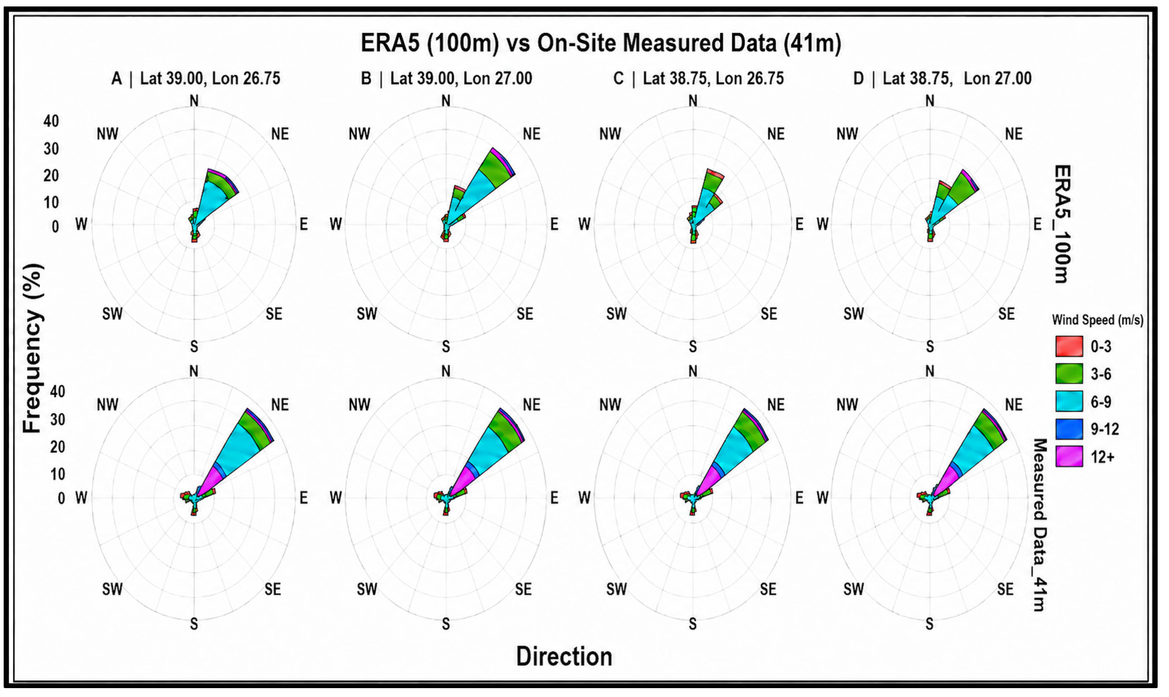
Comparative analyses between ERA5 reanalysis outputs and offshore measurement data demonstrated that ERA5 successfully represented the dominant offshore wind direction and the general directional frequency structure of the study area. The directional consistency between ERA5 grid points and measured offshore data was particularly strong for grid cells located closer to the meteorological mast location. This result indicates that the multi-grid ERA5 approach provides a reliable basis for long-term offshore wind characterization studies in coastal transition regions. Figure 7 presents the wind rose distributions derived from the four surrounding ERA5 grid points and the corresponding in situ measurements. The purpose of this figure is not to provide a single point-to-point validation plot, but to illustrate the directional consistency and spatial variability of the ERA5 wind field around the offshore mast location. Therefore, all four ERA5 grid points were retained in the figure because the proposed long-term reconstruction framework used multi-grid ERA5 information rather than relying on a single nearest or interpolated grid-cell representation. The in situ wind rose is included as the observational reference, while the ERA5 panels demonstrate how consistently the surrounding reanalysis grid cells reproduce the dominant offshore wind direction.
Despite the overall directional agreement, ERA5 output produced relatively smoother wind speed distributions compared to the offshore measurements, particularly within higher wind speed classes. This behavior was attributed to the spatial averaging characteristics of gridded reanalysis datasets and their limited capability to fully represent local offshore acceleration effects and microscale roughness transitions. Nevertheless, ERA5 successfully captured the long-term offshore atmospheric variability and provided a robust meteorological basis for machine learning-based wind reconstruction analyses.
The reconstructed long-term wind regime demonstrated that the study area maintains persistent offshore wind characteristics over multi-decadal periods, supporting the long-term viability of offshore wind energy production within the Northern Aegean region. The reconstructed wind direction distributions also confirmed the strong dominance of the NE–E sector throughout the long-term analysis period.

3.3. Machine Learning-Based MCP Performance

Distributed Random Forest achieved the lowest out-of-fold RMSE for scalar 100 m wind speed and both horizontal wind components and was consequently selected for all three response-specific reconstruction tasks. For ws100_obs, the selected DRF model achieved RMSE = 1.969 m/s, MAE = 1.504 m/s, bias = −0.027 m/s and Pearson r = 0.884. The selected u100_obs model achieved RMSE = 2.269 m/s, MAE = 1.588 m/s, bias = 0.082 m/s and r = 0.919, whereas the selected v100_obs model achieved RMSE = 2.478 m/s, MAE = 1.789 m/s, bias = 0.072 m/s and r = 0.890. GBM and XGBoost also provided competitive performance, indicating that the relationship between the multi-grid ERA5 predictors and local offshore wind conditions contained substantial nonlinear structure. The complete cross-validated model comparison is presented in Table 4.
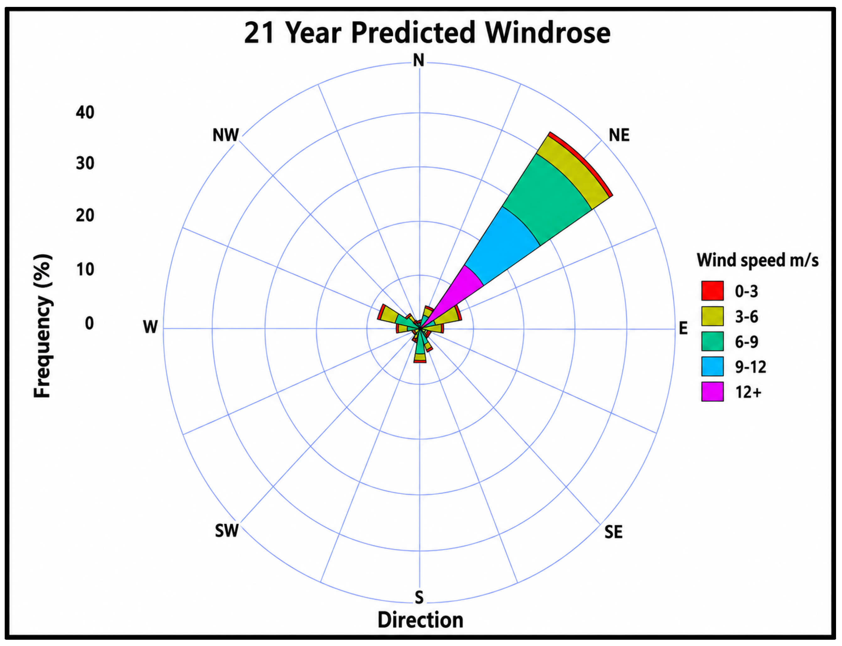
Wind direction reconstruction derived from the predicted u and v components also demonstrated satisfactory performance under offshore atmospheric conditions. The circular RMSE and circular MAE results indicated that the machine-learning-based framework successfully represented the dominant offshore directional structure despite the inherent complexity of circular variables. Compared with conventional linear MCP methods, the proposed approach provided improved reconstruction capability, particularly in capturing nonlinear atmospheric relationships and directional persistence. The long-term wind rose reconstructed using the machine-learning-based MCP framework is presented in Figure 8. The reconstructed 21-year wind climate preserved the dominant NE–E directional pattern observed during the measurement period, demonstrating the capability of the proposed approach to represent long-term offshore wind characteristics.
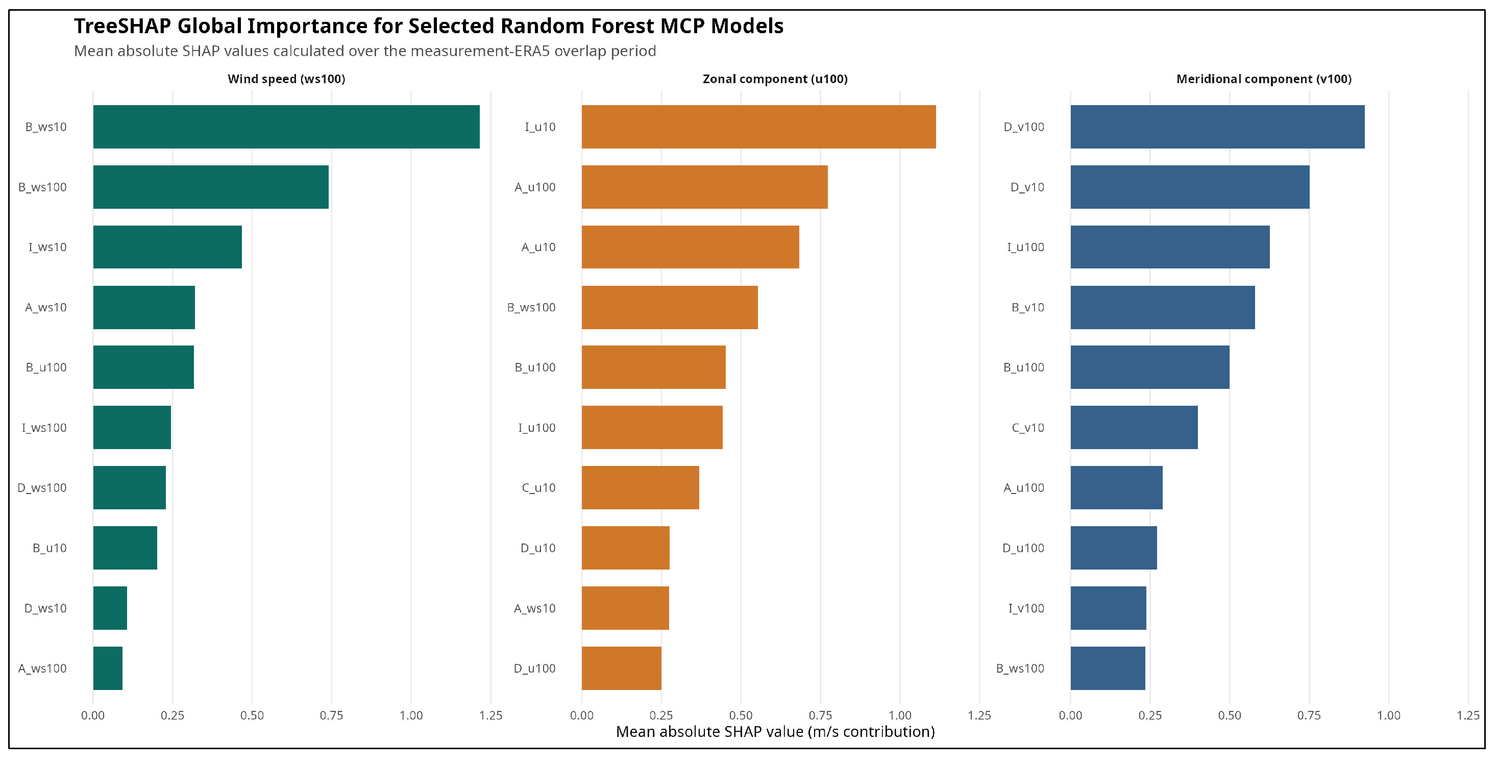
TreeSHAP analysis provided a robust model-specific interpretation of the three selected DRF models and confirmed that wind-related predictors dominated the reconstruction. For ws100_obs, B_ws10 was the leading predictor, followed by B_ws100 and I_ws10. For u100_obs, the bilinearly interpolated 10 m zonal component I_u10 had the highest mean absolute SHAP contribution, followed by A_u100 and A_u10. For v100_obs, D_v100 was the leading predictor, followed by D_v10 and I_u100. The leading predictors identified by TreeSHAP were consistent with the dominant variables identified by the earlier Random Forest ranking, while avoiding reliance on split-based importance alone. The global TreeSHAP importance distributions for the three selected DRF models are presented in Figure 9.

3.4. CFD Simulation and Wind Farm Layout Optimization

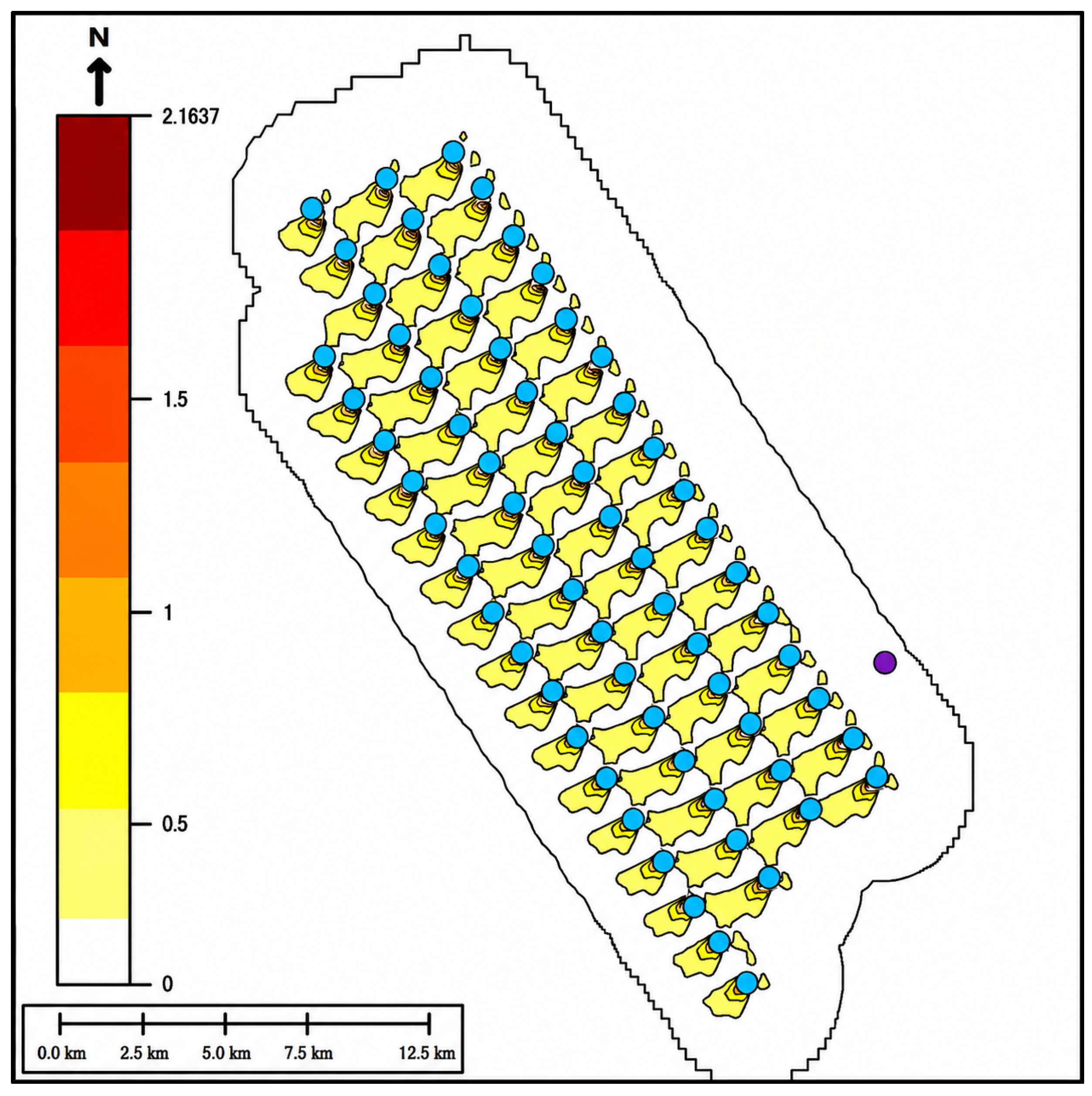
The optimization of turbine locations represents one of the most critical stages in offshore wind farm development, as overall energy production is governed not only by the available wind resource but also by turbine-to-turbine aerodynamic interactions. While high mean wind speeds are essential for maximizing energy yield, the spatial arrangement of turbines strongly influences wake formation and the resulting power losses throughout the wind farm. As air passes through a wind turbine rotor, kinetic energy is extracted from the flow, generating a downstream wake characterized by reduced wind speed and increased turbulence intensity. Consequently, turbines operating within the wake region of upstream turbines are exposed to less favorable inflow conditions, leading to reductions in power production and increased structural loading. The importance of minimizing these wake effects through appropriate turbine spacing and alignment is illustrated in Figure 10, which presents the optimized wind farm layout together with the corresponding wake-deficit zones. Figure 10 should be interpreted as a sector-based wake-deficit representation for the dominant NE–E offshore wind regime rather than as the result of a single fixed inflow direction. Because the dominant wind climate covers a directional sector instead of one exact direction, localized weak deficit areas may appear near the nominal upstream boundary of the wind farm. These small patches are related to directional-sector averaging and wake-field interpolation among neighbouring inflow directions and do not indicate physically upstream wake propagation.
To minimize wake effects, turbine locations were optimized according to the dominant NE–E wind regime identified from the measurement campaign and long-term wind climate reconstruction. Wake interactions were modelled using WindSim Wake Model 3, based on the analytical wake formulation developed by Takeshi Ishihara and co-workers. The model accounts for turbulence-dependent wake expansion to estimate downstream wind speed deficits and turbine-to-turbine wake losses. The final micrositing layout employed turbine spacings of approximately 5 rotor diameters (5D) in the cross-wind direction and 8 rotor diameters (8D) in the prevailing wind direction, ensuring adequate separation while maximizing the use of the available offshore area. There is no single fixed turbine-spacing standard for offshore wind farms, as spacing depends on the prevailing wind direction, wake-loss tolerance, project boundary constraints, turbine size, support structure and electrical layout. However, conventional offshore wind farm layouts are commonly expressed in terms of rotor diameters (D). Previous offshore wind siting assessments and wind farm layout studies indicate that spacing values of approximately 7D–10D along the prevailing wind direction and 3D–7D in the perpendicular or cross-wind direction are commonly considered in practice [66,67]. Therefore, the 5D cross-wind and 8D prevailing-wind spacing adopted in this study falls within the conventional offshore wind farm spacing range while reflecting the spatial limitations of the available Turkish territorial-water area and the dominant NE–E offshore wind regime. As shown in Figure 10, the wake-interaction indicator suggests that the main wake-affected zones remain largely confined between turbine rows and do not substantially overlap with downstream rotor-swept areas. This indicates that the adopted turbine arrangement effectively reduces wake interactions under dominant flow conditions, contributing to the relatively low overall wake losses estimated for the wind farm. To quantify these interactions, the spatial distribution of wake-induced wind speed deficits at the 170 m hub-height level is presented in Figure 11. Figure 10 and Figure 11 present two complementary wake-related outputs derived from the same WindSim Wake Model 3 assessment, but they should be interpreted differently. Figure 10 shows a wake-interaction indicator, which is used to visualize the spatial footprint of potential wake-affected zones across the optimized turbine layout. It is primarily a layout-scale diagnostic representation indicating where turbine-to-turbine wake interactions are expected to occur. In contrast, Figure 11 presents the quantitative wake-induced wind speed deficit at the 170 m hub-height level, expressed in m/s. Therefore, Figure 11 provides the magnitude of the local wind speed reduction over the CFD-derived ambient wind field and is more directly related to turbine-level wake exposure and energy-loss calculations. The spatial identification of individual turbines and their geographic coordinates are provided in Appendix A, while turbine-level wake-loss and energy-production results are summarized in Appendix B.
A detailed turbine-level assessment revealed significant differences in wake exposure across the wind farm. The spatial distribution of wake-induced wind speed deficits at the 170 m hub height level is presented in Figure 11.
Although the wake-deficit field is visually dominated by yellow tones, the deficit magnitude is not spatially uniform. The broader yellow areas indicate weak to moderate wake-induced wind speed reductions, while localized orange-to-red patches immediately downstream of individual turbine icons correspond to stronger wake effects. These high-deficit patches remain spatially limited and are mainly confined to the near-wake regions behind selected turbines.
The results indicate that wake effects are primarily concentrated within the downstream turbine rows aligned with the dominant offshore wind direction, while turbines located along the outer boundaries of the wind farm experience substantially lower flow interference. A detailed turbine-level assessment revealed significant differences in wake exposure across the wind farm. The highest wake loss was observed for Turbine 27, whose turbine ID and geographic coordinates are provided in Appendix A and whose turbine-level energy results are summarized in Appendix B. For this turbine, the wake-induced energy loss reached 8.468%. The gross annual energy production was calculated as 88.442 GWh/year, decreasing to 80.952 GWh/year after accounting for wake effects. This result indicates that Turbine 27 is located within a region more strongly affected by upstream turbine wakes and flow deceleration caused by turbine-to-turbine interactions. In contrast, the lowest wake loss was observed for Turbine 50, which is also identifiable through the turbine-ID coordinate list in Appendix A and the turbine-level energy table in Appendix B. For this turbine, the wake loss was only 0.505%, with gross annual energy production of 87.852 GWh/year and wake-adjusted annual energy production of 87.408 GWh/year. The relatively small energy reduction indicates that Turbine 50 occupies a favorable position within the wind farm layout and is only minimally influenced by upstream wake effects.

3.5. Wind Farm Energy Production Assessment

The CFD simulations successfully represented the offshore wind flow structure and spatial wind speed variability across the study area. The numerical solutions demonstrated stable convergence behavior and the monitored residuals and spot values indicated numerically stable and converged solutions for all directional sectors. The offshore wind atlas generated from CFD simulations revealed relatively homogeneous offshore wind conditions over large portions of the project area, while localized wind speed variations were observed near coastal transition regions and terrain-induced flow interaction zones. The offshore sea surface provided relatively smooth aerodynamic conditions with reduced roughness effects, contributing to favorable offshore wind acceleration characteristics.
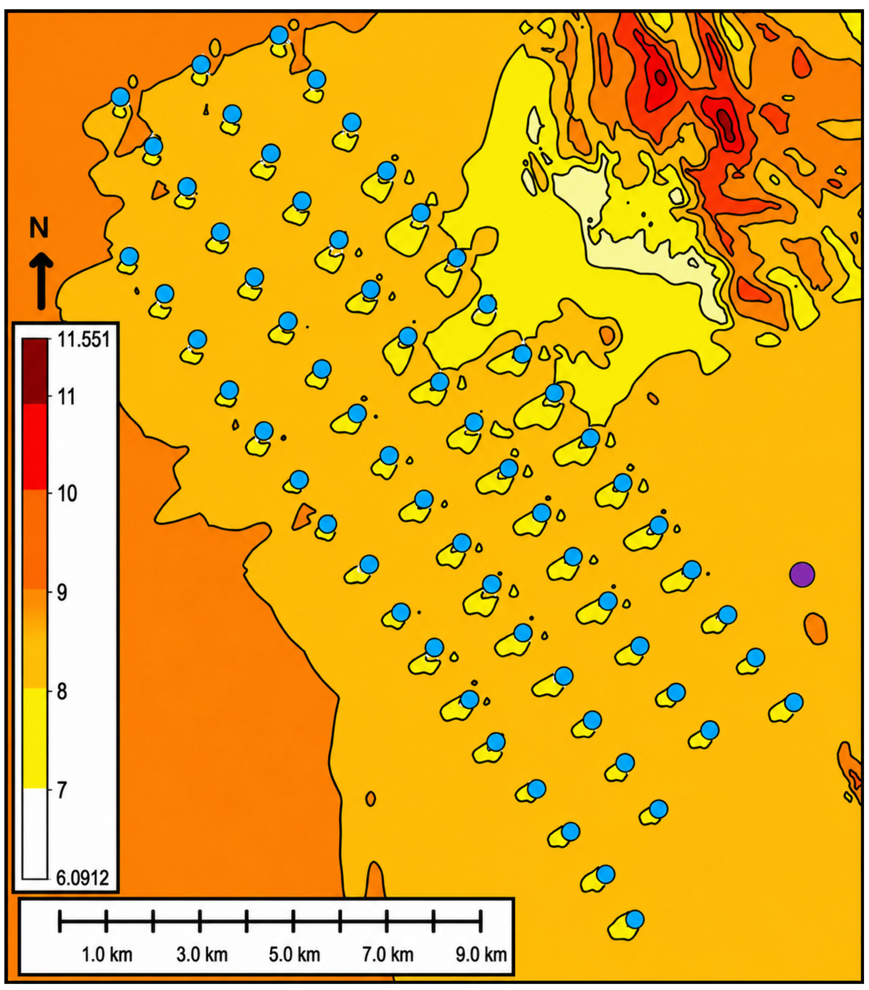
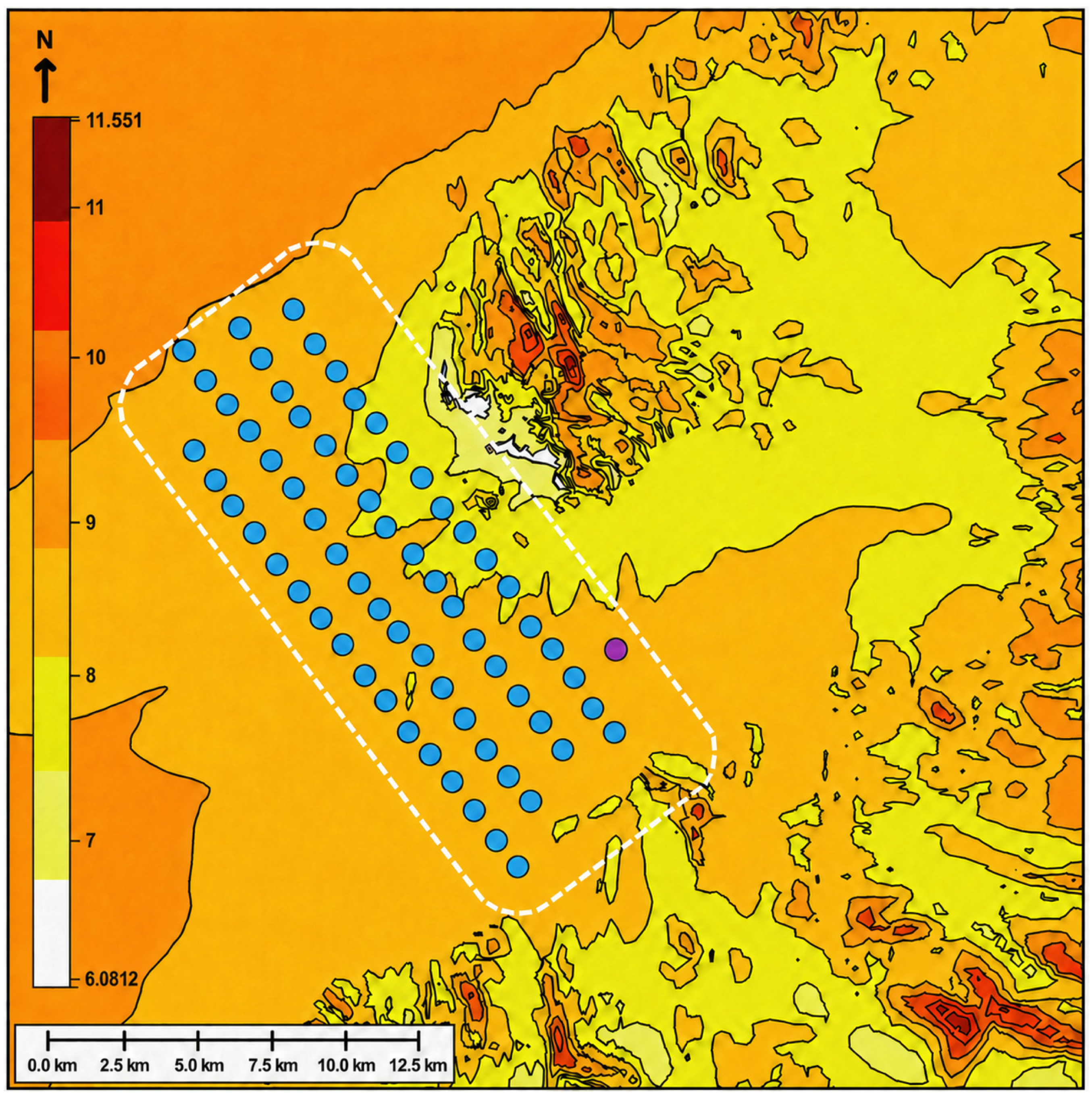
Figure 12 illustrates the final wind farm layout superimposed on the CFD-derived mean wind speed atlas. The turbine positions were determined through a micrositing process that considered the dominant NE–E wind regime, local wind resource distribution and wake-interaction effects. The resulting layout was designed to maximize energy production while minimizing wake-induced losses under prevailing offshore wind conditions.
The offshore wind farm energy analyses indicated that the proposed wind farm configuration possesses strong energy production potential under the reconstructed long-term offshore wind conditions. A summary of the wind farm configuration and the principal energy production metrics, including turbine specifications, installed capacity, annual energy production, wake losses, full-load hours and capacity factor, is presented in Table 5. The modeled wind farm consisted of 65 IEA-22-280-RWT reference turbines with a total installed capacity of 1430 MW. The gross annual energy production of the proposed offshore wind farm was calculated as 5794.8 GWh/year. When turbine-to-turbine wake interactions were included in the analyses, the total wake loss remained limited to approximately 5.2%, resulting in a wake-adjusted annual energy production of 5494.5 GWh/year. In addition, the wind farm achieved a full-load equivalent operating duration of 3842.3 h/year and an overall capacity factor of 43.9%, indicating highly favorable offshore operational performance. Detailed turbine-based analyses revealed that first-row turbines exposed directly to the dominant offshore airflow experienced relatively low wake losses, whereas turbines located within inner rows and central sections of the wind farm were subjected to stronger flow shadowing effects. The maximum wake loss was observed for turbines positioned within the central cluster aligned with the dominant offshore flow direction. These findings demonstrated the importance of turbine spacing and layout optimization in minimizing wake-induced production losses under offshore atmospheric conditions. The obtained energy production characteristics indicate that the proposed offshore wind farm configuration could make a substantial contribution to the renewable energy capacity of Türkiye and support long-term low-carbon energy transition objectives.

4. Conclusions and Discussion

The in situ measurement results confirm that the Northern Aegean study area is characterized by a strong and directionally persistent marine wind climate. The measured wind-speed level, low vertical shear and stable Weibull distribution indicate favorable offshore atmospheric conditions for large-scale wind energy development. These findings agree with regional assessments identifying the central and eastern Aegean Sea as areas of high wind potential and comparatively low variability [68]. They are also consistent with buoy-based Weibull analyses conducted across the Aegean Sea [69,70]. This agreement supports both the representativeness of the measurement campaign and the suitability of the Northern Aegean Sea for utility-scale offshore wind development.
The ERA5 successfully reproduced the dominant wind direction and general directional frequency structure observed at the site. This result is consistent with studies demonstrating the usefulness of reanalysis data for regional offshore wind characterization in the Greek Seas and wider Aegean region [71,72]. However, ERA5 produced smoother distributions in the higher wind speed classes. Similar underestimations of strong winds and local-scale variability have been reported [73]. Such differences are expected because the spatial averaging inherent in gridded reanalysis products cannot fully resolve coastal acceleration, land–sea roughness transitions and other site-specific flow effects. The simultaneous use of four surrounding ERA5 grid points, therefore, provided a broader atmospheric representation than a single-grid approach, while the ML-based MCP procedure transferred this regional information toward the measured local wind climate.
The ML results further demonstrate the value of nonlinear methods for long-term offshore wind data reconstruction. Distributed Random Forest provided the lowest out-of-fold RMSE for 100 m wind speed, with RMSE = 1.969 m/s, Pearson r = 0.884 and negligible aggregate bias. This result agrees with previous studies showing that ERA5-driven ML models can improve hub-height wind representation compared with direct reanalysis estimates [74]. The strong performance of RF in the present study indicates that the model effectively captured nonlinear relationships between the ERA5 predictors and site-specific offshore wind conditions. TreeSHAP analysis confirmed that the most influential variables were physically relevant wind-speed and component predictors: B_ws10 for scalar speed, I_u10 for the zonal component and D_v100 for the meridional component. The agreement between TreeSHAP and the earlier Random Forest ranking strengthens confidence that the reported spatial and vertical predictor patterns were model-consistent rather than artifacts of a single split-based importance measure. Atmospheric predictors such as boundary-layer height, humidity, temperature, pressure and air density contributed additional information but exhibited lower global SHAP magnitudes than the principal wind variables [55,75]. GBM and XGBoost also produced competitive results, consistent with studies showing that boosting methods improve wind predictions through iterative residual corrections [76,77]. Although LSTM-based models have achieved strong performance in short-term forecasting [78,79], their larger data and computational requirements make ensemble tree-based approaches more practical for long-term reconstruction from a limited on-site measurement period.
Another strength of the framework is the use of a multidimensional ERA5 predictor set. Offshore wind variability is influenced not only by wind speed and direction but also by atmospheric stability, thermal stratification, boundary-layer development, pressure gradients, moisture and surface–atmosphere exchange. Accordingly, temperature, pressure, boundary-layer height, humidity-related parameters and other atmospheric descriptors were evaluated with wind variables. The feature-importance results were physically consistent with previous findings showing that atmospheric stability influences offshore and coastal wind-resource characteristics [80]. Model training and validation were conducted using a Leave-One-Month-Out cross-validation strategy, in which each complete month was successively excluded from model training and used as an independent test period. This temporally blocked procedure was adopted to reduce information leakage associated with autocorrelated observations and to evaluate model robustness across different seasonal conditions [81].
The benefit of a broader atmospheric description is also supported by the recent literature. Hallgren et al. showed that boundary-layer-related variables improved the prediction of coastal wind profiles and low-level jets [82], while ElTaweel et al. obtained higher accuracy by combining multiple ERA5 predictors in tree-based models [83]. Additional reanalysis-based studies reported gains from enriched meteorological input sets in the RF and LightGBM frameworks [84,85]. Recent forecasting studies and reviews likewise emphasize that thermodynamic and multiscale meteorological information can help ML models capture nonlinear wind variability more effectively [86,87]. Therefore, the improved reconstruction in the present study should be attributed to the combination of suitable algorithms and a physically informed atmospheric predictor set, rather than to the algorithm choice alone.
CFD simulations complemented the long-term reconstruction by resolving microscale wind variability across the offshore domain. High-resolution terrain and surface roughness inputs allowed the model to distinguish between the marine surface, coastal transition zones and rougher onshore terrain. The resulting wind atlas showed a relatively homogeneous offshore flow over much of the project area, with localized modifications near the coastal and terrain-interaction zones. These results demonstrate the importance of coupling long-term atmospheric reconstruction with microscale modelling, since reanalysis data characterize the regional climate, whereas CFD provides the spatial detail required for turbine micrositing and wake-aware layout design.
The optimized 65-turbine configuration, based on the IEA-22-280-RWT reference turbine, had a total installed capacity of 1430 MW. The gross annual energy production was estimated to be 5794.8 GWh/year. After accounting for turbine-to-turbine wake interactions, the wake loss remained approximately 5.2%, yielding a wake-adjusted energy production of 5494.5 GWh/year and a capacity factor of 43.9%. Wake losses were higher for turbines located within the inner rows and along the dominant flow axis; however, the farm-wide loss remained moderate for a project of this scale. This indicates that the micrositing strategy achieved an effective balance between spatial utilization, aerodynamic exposure and wake mitigation.
The wake-adjusted capacity factor was also consistent with published assessments for the Aegean Sea. Reported values range from 27.4% at Athos to 47.3% at Mykonos [70], while estimates of 38.5–41.0% and 44.7% have been reported for sites near Limnos [88,89]. For the Turkish Aegean coast, capacity factors of 47.3% near Bozcaada [90], 43–46% in the Gulf of Edremit [28] and up to 51.8% at Foça [32] were reported. A recent CERRA-based assessment produced theoretical values between 28.7% and 54.9% across the proposed Greek offshore development areas [91]. The value of 43.9% obtained here lies within the upper-middle range of regional estimates. However, direct comparisons require caution because the studies differ in turbine technology, hub height, reanalysis product, spatial resolution and loss assumptions.
An important distinction is that the present capacity factor represents the wake-adjusted output of the complete 65-turbine wind farm, whereas several regional studies report theoretical or single-turbine values without cumulative wake, electrical, or availability losses. The resulting 43.9% capacity factor indicates favorable operational performance under a comparatively realistic farm-scale configuration. Further project development should include complete electrical, availability, environmental and operational loss assessments, as well as validation against longer offshore measurement records. A formal quantitative uncertainty budget was not calculated in this study, and no uncertainty coefficients, confidence intervals, or P50/P75/P90 energy estimates are reported. The main uncertainty sources are associated with ERA5 representation, machine-learning reconstruction, vertical extrapolation, CFD assumptions, wake modelling and their combined influence on AEP. Therefore, the reported energy results should be interpreted as scenario-based engineering estimates rather than bankable yield values. A complete uncertainty assessment would require longer offshore measurements, independent validation datasets, ensemble simulations and formal uncertainty propagation.
Overall, the integrated framework provides a technically robust basis for offshore wind assessments under limited observational conditions. The combination of on-site measurements, multi-grid and multi-parameter ERA5 data, ML-based MCP reconstruction and CFD-supported micrositing reduced the limitations of using any single method in isolation. The estimated wake-adjusted energy production of approximately 5.49 TWh/year also demonstrates the potential contribution of a single, large-scale offshore project to Türkiye’s renewable electricity portfolio. This methodology can support future investment screening, marine spatial planning and offshore wind policy development in Türkiye and other data-scarce coastal regions with comparable atmospheric and geographic characteristics.

Author Contributions

Conceptualization: C.T., V.Y. and H.T.; methodology: C.T., C.Ö. and V.Y.; validation: Y.K. and C.Ö.; formal analysis: C.T.; resources: Y.K.; writing—original draft: C.T. and V.Y.; writing—review & editing: V.Y.; supervision: V.Y. and H.T. All authors have read and agreed to the published version of the manuscript.

Funding

This research received no external funding.

Institutional Review Board Statement

Not applicable.

Informed Consent Statement

Not applicable.

Data Availability Statement

The data used in this study are not publicly available because they are subject to licensing restrictions imposed by the İzmir Development Agency (İZKA). Access may be granted upon reasonable request to the corresponding author and subject to approval by İZKA.

Acknowledgments

The offshore wind measurement data used in this study were provided by the Izmir Development Agency (İZKA). All rights belong to İZKA. The authors would like to thank the İzmir Development Agency (İZKA) for its support.

Conflicts of Interest

The authors declare no conflicts of interest.

Appendix A. Wind Turbine Coordinate List (UTM GWS 84)

Turbine No.Hub Height (m)Easting (m)Northing (m)
1170.0489,485.04,298,453.0
2170.0488,617.04,299,573.0
3170.0487,725.04,300,673.0
4170.0486,854.04,301,804.0
5170.0486,015.04,302,946.0
6170.0485,144.04,304,058.0
7170.0484,293.04,305,206.0
8170.0483,408.04,306,317.0
9170.0482,553.04,307,443.0
10170.0481,698.04,308,581.0
11170.0480,824.04,309,701.0
12170.0479,981.04,310,835.0
13170.0479,091.04,311,948.0
14170.0478,228.04,313,063.0
15170.0477,354.04,314,188.0
16170.0476,491.04,315,313.0
17170.0487,347.04,297,682.0
18170.0486,489.04,298,755.0
19170.0485,580.04,299,898.0
20170.0484,715.04,301,023.0
21170.0483,870.04,302,164.0
22170.0482,999.04,303,296.0
23170.0482,133.04,304,416.0
24170.0481,268.04,305,544.0
25170.0480,408.04,306,676.0
26170.0479,553.04,307,803.0
27170.0478,680.04,308,925.0
28170.0477,820.04,310,045.0
29170.0476,951.04,311,169.0
30170.0476,076.04,312,287.0
31170.0475,207.04,313,417.0
32170.0474,348.04,314,552.0
33170.0486,123.04,295,762.0
34170.0485,205.04,296,851.0
35170.0484,354.04,297,979.0
36170.0483,448.04,299,076.0
37170.0482,581.04,300,208.0
38170.0481,741.04,301,343.0
39170.0480,873.04,302,468.0
40170.0480,001.04,303,597.0
41170.0479,138.04,304,718.0
42170.0478,282.04,305,847.0
43170.0477,430.04,306,983.0
44170.0476,553.04,308,113.0
45170.0475,690.04,309,233.0
46170.0474,824.04,310,356.0
47170.0473,950.04,311,469.0
48170.0473,082.04,312,605.0
49170.0472,223.04,313,732.0
50170.0485,477.04,292,965.0
51170.0484,621.04,294,114.0
52170.0483,703.04,295,195.0
53170.0482,856.04,296,322.0
54170.0481,949.04,297,413.0
55170.0481,071.04,298,528.0
56170.0480,232.04,299,681.0
57170.0479,367.04,300,801.0
58170.0478,489.04,301,926.0
59170.0477,615.04,303,045.0
60170.0476,770.04,304,179.0
61170.0475,908.04,305,306.0
62170.0475,038.04,306,431.0
63170.0474,174.04,307,550.0
64170.0473,310.04,308,683.0
65170.0472,432.04,309,796.0

Appendix B. Annual Energy Production per Wind Turbine

Turbine NoAir Density (kg/m3)Average Wind Speed (m/s)Gross AEP (GWh/Year)Wake Losses (%)Wake-Adjusted AEP (GWh/Year)
11.1908.33088.5940.70587.969
21.1908.44090.0921.01689.176
31.1908.34088.4821.66587.009
41.1908.34088.5491.69387.050
51.1908.20086.3771.84784.782
61.1908.10084.2091.89082.618
71.1907.98081.9362.12580.195
81.1907.85080.6122.08378.933
91.1908.03083.7402.04182.031
101.1907.58076.3372.40474.502
111.1908.00084.5202.00282.827
121.1908.00084.6862.27782.757
131.1908.10086.8772.05085.096
141.1908.38091.7331.87890.011
151.1908.52093.6171.80291.930
161.1908.63095.3861.11494.324
171.1908.39089.4414.29185.603
181.1908.47090.3497.11283.924
191.1908.37088.7867.04482.533
201.1908.23087.0737.26680.746
211.1908.24086.9237.23980.631
221.1908.18085.3356.73179.591
231.1908.12085.1246.97879.184
241.1908.15086.0927.12979.954
251.1908.03084.1087.79677.551
261.1908.18087.8547.51581.252
271.1908.20088.4428.46880.952
281.1908.21088.4718.03081.367
291.1908.35091.0458.43583.365
301.1908.40091.7007.98784.375
311.1908.54093.5977.74186.352
321.1908.68095.3623.64291.889
331.1908.46090.7514.29986.850
341.1908.41089.6768.05482.453
351.1908.40089.0427.31382.531
361.1908.29087.4248.03380.401
371.1908.23086.8427.55480.282
381.1908.17085.3947.48279.004
391.1908.25086.7377.55580.184
401.1908.29088.7437.59082.008
411.1908.32088.4657.36681.949
421.1908.25089.4838.38481.981
431.1908.43091.9437.75284.815
441.1908.32090.8928.25083.393
451.1908.43092.7348.29385.044
461.1908.49093.4868.27885.748
471.1908.56094.3997.47587.343
481.1908.65095.3937.25388.474
491.1908.74096.1123.31092.931
501.1908.20087.8520.50587.408
511.1908.36089.6463.63486.388
521.1908.47090.5784.46686.534
531.1908.43089.5904.74885.336
541.1908.28086.9014.41083.069
551.1908.21085.9904.21882.363
561.1908.25086.9453.83883.608
571.1908.36088.8174.27785.019
581.1908.46091.1124.94986.603
591.1908.45091.6894.17087.866
601.1908.57093.9055.98688.284
611.1908.37091.5064.37387.504
621.1908.55094.2155.61188.928
631.1908.47093.5444.89788.963
641.1908.53094.2864.92489.644
651.1908.60095.2434.31291.135

References

  1. Gielen, D.; Boshell, F.; Saygin, D.; Bazilian, M.D.; Wagner, N.; Gorini, R. The Role of Renewable Energy in the Global Energy Transformation. Energy Strategy Rev. 2019, 24, 38–50. [Google Scholar] [CrossRef] [Scilit]
  2. Kabeyi, M.J.B.; Olanrewaju, O.A. Sustainable Energy Transition for Renewable and Low Carbon Grid Electricity Generation and Supply. Front. Energy Res. 2022, 9, 743114. [Google Scholar] [CrossRef] [Scilit]
  3. Obiora, S.; Bamisile, O.; Hu, Y.; Ozsahin, D.; Adun, H. Assessing the Decarbonization of Electricity Generation in Major Emitting Countries by 2030 and 2050: Transition to a High Share Renewable Energy Mix. Heliyon 2024, 10, e28770. [Google Scholar] [CrossRef] [Scilit]
  4. Tumse, S.; Bilgili, M.; Yıldırım, A.; Şahin, B. Comparative Analysis of Global Onshore and Offshore Wind Energy Characteristics and Potentials. Sustainability 2024, 16, 6614. [Google Scholar] [CrossRef] [Scilit]
  5. Esteban, M.D.; Diez, J.J.; López, J.S.; Negro, V. Why Offshore Wind Energy. Renew. Energy 2011, 36, 444–450. [Google Scholar] [CrossRef] [Scilit]
  6. Kaldellis, J.K.; Kapsali, M. Shifting towards Offshore Wind Energy—Recent Activity and Future Development. Energy Policy 2013, 53, 136–148. [Google Scholar] [CrossRef] [Scilit]
  7. Global Wind Energy Council. Global Wind Report 2025; Global Wind Energy Council: Brussels, Belgium, 2025. [Google Scholar]
  8. Global Wind Energy Council. Global Offshore Wind Report 2025; Global Wind Energy Council: Brussels, Belgium, 2025. [Google Scholar]
  9. Bogdanov, D.; Ram, M.; Aghahosseini, A.; Gulagi, A.; Oyewo, A.S.; Child, M.; Caldera, U.; Sadovskaia, K.; Farfan, J.; Barbosa, L.S.N.S.; et al. Low-Cost Renewable Electricity as the Key Driver of the Global Energy Transition towards Sustainability. Energy 2021, 227, 120467. [Google Scholar] [CrossRef] [Scilit]
  10. Wen, Y.; Wu, J.; Lin, P.; Low, Y.M. The Role of Offshore Wind and Solar PV Resources in Global Low-Carbon Transition. Sci. Adv. 2025, 11, adx5580. [Google Scholar] [CrossRef] [Scilit]
  11. Keivanpour, S.; Ramudhin, A.; Ait Kadi, D. The Sustainable Worldwide Offshore Wind Energy Potential: A Systematic Review. J. Renew. Sustain. Energy 2017, 9, 065902. [Google Scholar] [CrossRef] [Scilit]
  12. Tanvir, M.S.; Etminan, A. Comparative Analysis of Offshore and Onshore Wind Turbines: Efficiency, Design, and Environmental Impact. Wind Eng. 2025, 50, 200–215. [Google Scholar] [CrossRef] [Scilit]
  13. Kumar, P.; Paul, S.; Saha, A.K.; Yadav, O. Recent Advancements in Planning and Reliability Aspects of Large-Scale Deep Sea Offshore Wind Power Plants: A Review. IEEE Access 2025, 13, 3738–3767. [Google Scholar] [CrossRef] [Scilit]
  14. Gulaydin, O.; Mourshed, M. Net-Zero Turkey: Renewable Energy Potential and Implementation Challenges. Energy Sustain. Dev. 2025, 87, 101744. [Google Scholar] [CrossRef] [Scilit]
  15. T.C. Çevre, Şehircilik ve İklim Değişikliği Bakanlığı. 2053 Uzun Dönemli İklim Stratejisi; T.C. Çevre, Şehircilik ve İklim Değişikliği Bakanlığı: Ankara, Türkiye, 2024. (In Turkish)
  16. T.C. Enerji ve Tabii Kaynaklar Bakanlığı. Enerji Dönüşümü: Yenilenebilir Enerji 2035; T.C. Çevre, Şehircilik ve İklim Değişikliği Bakanlığı: Ankara, Türkiye, 2024. (In Turkish)
  17. World Bank. Offshore Wind Roadmap for Türkiye; World Bank: Washington, DC, USA, 2024. [Google Scholar]
  18. Badger, M.; Hasager, C.; Hahmann, A.; Volker, P.; di Bella, A.; Bingöl, F. ESA ResGrow: Trial Cases for SAR Lifting: Aegean Sea; DTU Wind Energy Report-I-0375; DTU Wind Energy, Technical University of Denmark: Roskilde, Denmark, 2015. [Google Scholar]
  19. Hersbach, H.; Bell, B.; Berrisford, P.; Hirahara, S.; Horányi, A.; Muñoz-Sabater, J.; Nicolas, J.; Peubey, C.; Radu, R.; Schepers, D.; et al. The ERA5 global reanalysis. Q. J. R. Meteorol. Soc. 2020, 146, 1999–2049. [Google Scholar] [CrossRef] [Scilit]
  20. Argin, M.; Yerci, V. The assessment of offshore wind power potential of Turkey. In Proceedings of the 2015 9th International Conference on Electrical and Electronics Engineering (ELECO), Bursa, Türkiye, 26–28 November 2015; IEEE: Piscataway, NJ, USA, 2015; pp. 966–970. [Google Scholar] [CrossRef] [Scilit]
  21. Argin, M.; Yerci, V.; Erdogan, N.; Kucuksari, S.; Cali, U. Exploring the offshore wind energy potential of Turkey based on multi-criteria site selection. Energy Strategy Rev. 2019, 23, 33–46. [Google Scholar] [CrossRef] [Scilit]
  22. Genç, M.S.; Karipoğlu, F.; Koca, K.; Azgın, Ş.T. Suitable site selection for offshore wind farms in Turkey’s seas: GIS-MCDM based approach. Earth Sci. Inform. 2021, 14, 1213–1225. [Google Scholar] [CrossRef] [Scilit]
  23. Oguz, E.; Akgul, M.A.; Incecik, A. Offshore wind farms: Potential and applicability in the Southern Marmara Region, Turkey. In Developments in Maritime Transportation and Exploitation of Sea Resources: Proceedings of IMAM 2013, 15th International Congress of the International Maritime Association of the Mediterranean; Guedes Soares, C., López Peña, F., Eds.; Taylor & Francis Group: London, UK, 2014; pp. 943–949. [Google Scholar]
  24. Cali, U.; Erdogan, N.; Kucuksari, S.; Argin, M. Techno-economic analysis of high potential offshore wind farm locations in Turkey. Energy Strategy Rev. 2018, 22, 325–336. [Google Scholar] [CrossRef] [Scilit]
  25. Aslan, A. Comparison based on the technical and economical analysis of wind energy potential at onshore, coastal, and offshore locations in Çanakkale, Turkey. J. Renew. Sustain. Energy 2020, 12, 063306. [Google Scholar] [CrossRef] [Scilit]
  26. Karipoğlu, F.; Öztürk, S.; Genç, M.S. Determining suitable regions for potential offshore wind farms in Bandırma Bay using multi-criteria-decision-making method. Mühendis. Bilim. Araştırmaları Derg. 2021, 3, 123–132. [Google Scholar] [CrossRef] [Scilit]
  27. Güner, F.; Başer, V.; Zenk, H. Evaluation of offshore wind power plant sustainability: A case study of Sinop/Gerze, Turkey. Int. J. Glob. Warm. 2021, 23, 370–384. [Google Scholar] [CrossRef] [Scilit]
  28. Özbek, M.; Tunc, K.M.M. Feasibility of offshore wind energy in Turkey: A case study for Gulf of Edremit at the Aegean Sea. Gazi Univ. J. Sci. 2021, 34, 423–437. [Google Scholar] [CrossRef] [Scilit]
  29. Önden, İ.; Kara, K.; Yalçın, G.C.; Deveci, M.; Önden, A.; Eker, M. Strategic location analysis for offshore wind farms to sustainably fulfill railway energy demand in Turkey. J. Clean. Prod. 2024, 434, 140142. [Google Scholar] [CrossRef] [Scilit]
  30. Guliyev, J.; Güneri, B.; Konur, M.; Duymaz, Ş.; Türk, A. Offshore Wind Power Site Selection in Türkiye Using q-Rung Orthopair Fuzzy Sets and the COPRAS Method. J. Oper. Intell. 2025, 3, 283–307. [Google Scholar] [CrossRef] [Scilit]
  31. Gualtieri, G. Analysing the Uncertainties of Reanalysis Data Used for Wind Resource Assessment: A Critical Review. Renew. Sustain. Energy Rev. 2022, 167, 112741. [Google Scholar] [CrossRef] [Scilit]
  32. Duzcan, A.; Kara, Y. Offshore Wind Energy Potential Analysis of Turkish Marmara and Aegean Seas. Int. J. Environ. Sci. Technol. 2023, 20, 5571–5584. [Google Scholar] [CrossRef] [Scilit]
  33. Başaran, H.; Tarhan, İ. Investigation of Offshore Wind Characteristics for the Northwest of Türkiye Region by Using Multi-Criteria Decision-Making Method (MOORA). Results Eng. 2022, 16, 100757. [Google Scholar] [CrossRef] [Scilit]
  34. Aksu, E.Ö.; Gencer, C.T. GIS-Based Optimum Location Selection for Offshore Wind Energy: A Case Study for Turkey. Ocean Eng. 2025, 320, 120292. [Google Scholar] [CrossRef] [Scilit]
  35. Carta, J.A.; Velázquez, S.; Cabrera, P. A Review of Measure-Correlate-Predict (MCP) Methods Used to Estimate Long-Term Wind Characteristics at a Target Site. Renew. Sustain. Energy Rev. 2013, 27, 362–400. [Google Scholar] [CrossRef] [Scilit]
  36. Amarzaya, B.; Ko, K. Effect of Wind Measurement Period and Data Recovery Rate on Performance of Measure-Correlate-Predict Method with Machine Learning. J. Mech. Sci. Technol. 2025, 39, 4355–4364. [Google Scholar] [CrossRef] [Scilit]
  37. Rouholahnejad, F.; Gottschall, J. Characterization of Local Wind Profiles: A Random Forest Approach for Enhanced Wind Profile Extrapolation. Wind Energy Sci. 2025, 10, 143–159. [Google Scholar] [CrossRef] [Scilit]
  38. Sickler, M.; Ummels, B.; Zaaijer, M.; Schmehl, R.; Dykes, K. Offshore Wind Farm Optimisation: A Comparison of Performance between Regular and Irregular Wind Turbine Layouts. Wind Energy Sci. 2023, 8, 1225–1233. [Google Scholar] [CrossRef] [Scilit]
  39. Wang, G.; Huang, J.; Zhang, Z.; Chen, K.; Shen, Z.; Tu, J.; Han, Z. Influence of Layout on Offshore Wind Farm Efficiency and Wake Characteristics in Turbulent Environments. J. Mar. Sci. Eng. 2025, 13, 2137. [Google Scholar] [CrossRef] [Scilit]
  40. Rasiński, A.; Malecha, Z. Wake Losses, Productivity, and Cost Analysis of a Polish Offshore Wind Farm in the Baltic Sea. Energies 2025, 18, 4190. [Google Scholar] [CrossRef] [Scilit]
  41. Baptista, J.; Jesus, B.; Cerveira, A.; Pires, E. Offshore Wind Farm Layout Optimisation Considering Wake Effect and Power Losses. Sustainability 2023, 15, 9893. [Google Scholar] [CrossRef] [Scilit]
  42. Dafka, S.; Toreti, A.; Luterbacher, J.; Zanis, P.; Tyrlis, E.; Xoplaki, E. Simulating Extreme Etesians over the Aegean and Implications for Wind Energy Production in Southeastern Europe. J. Appl. Meteorol. Climatol. 2018, 57, 1123–1134. [Google Scholar] [CrossRef] [Scilit]
  43. Gualtieri, G. Reliability of ERA5 Reanalysis Data for Wind Resource Assessment: A Comparison against Tall Towers. Energies 2021, 14, 4169. [Google Scholar] [CrossRef] [Scilit]
  44. Hayes, L.; Stocks, M.; Blakers, A. Accurate Long-Term Power Generation Model for Offshore Wind Farms in Europe Using ERA5 Reanalysis. Energy 2021, 229, 120603. [Google Scholar] [CrossRef] [Scilit]
  45. Gandoin, R.; Garza, J. Underestimation of Strong Wind Speeds Offshore in ERA5: Evidence, Discussion and Correction. Wind Energy Sci. 2024, 9, 1727–1745. [Google Scholar] [CrossRef] [Scilit]
  46. Miao, H.; Dong, D.; Huang, G.; Hu, K.; Tian, Q.; Gong, Y. Evaluation of Northern Hemisphere Surface Wind Speed and Wind Power Density in Multiple Reanalysis Datasets. Energy 2020, 208, 117382. [Google Scholar] [CrossRef] [Scilit]
  47. Gualtieri, G.; Secci, S. Methods to Extrapolate Wind Resource to the Turbine Hub Height Based on Power Law: A 1-h Wind Speed vs. Weibull Distribution Extrapolation Comparison. Renew. Energy 2012, 43, 183–200. [Google Scholar] [CrossRef] [Scilit]
  48. Golbazi, M.; Archer, C.L. Surface Roughness for Offshore Wind Energy. J. Phys. Conf. Ser. 2020, 1452, 012024. [Google Scholar] [CrossRef] [Scilit]
  49. Ryu, G.-H.; Kim, D.; Kim, D.-Y.; Kim, Y.-G.; Kwak, S.J.; Choi, M.S.; Jeon, W.; Kim, B.-S.; Moon, C.-J. Analysis of Vertical Wind Shear Effects on Offshore Wind Energy Prediction Accuracy Applying Rotor Equivalent Wind Speed and the Relationship with Atmospheric Stability. Appl. Sci. 2022, 12, 6949. [Google Scholar] [CrossRef] [Scilit]
  50. Houndekindo, F.; Ouarda, T.B.M.J. Machine Learning and Statistical Approaches for Wind Speed Estimation at Partially Sampled and Unsampled Locations: Review and Open Questions. Energy Convers. Manag. 2025, 327, 119555. [Google Scholar] [CrossRef] [Scilit]
  51. Mifsud, M.D.; Sant, T.; Farrugia, R.N. Analysing Uncertainties in Offshore Wind Farm Power Output Using Measure-Correlate-Predict Methodologies. Wind Energy Sci. 2020, 5, 601–621. [Google Scholar] [CrossRef] [Scilit]
  52. Özen, C.; Dinç, U.; Deniz, A.; Karan, H. Wind Power Generation Forecast by Coupling Numerical Weather Prediction Model and Gradient Boosting Machines in Yahyalı Wind Power Plant. Wind Eng. 2021, 45, 1256–1272. [Google Scholar] [CrossRef] [Scilit]
  53. Ferreira, L.; Pilastri, A.; Martins, C.; Pires, P.M.; Cortez, P. A Comparison of AutoML Tools for Machine Learning, Deep Learning and XGBoost. In Proceedings of the 2021 International Joint Conference on Neural Networks (IJCNN), Shenzhen, China, 18–22 July 2021; IEEE: Piscataway, NJ, USA, 2021; pp. 1–8. [Google Scholar] [CrossRef] [Scilit]
  54. Özen, C.; Deniz, A. A Comprehensive Country-Based Day-Ahead Wind Power Generation Forecast Model by Coupling Numerical Weather Prediction Data and CatBoost with Feature Selection Methods for Turkey. Wind Eng. 2022, 46, 1359–1388. [Google Scholar] [CrossRef] [Scilit]
  55. Lundberg, S.M.; Erion, G.; Chen, H.; DeGrave, A.; Prutkin, J.M.; Nair, B.; Katz, R.; Himmelfarb, J.; Bansal, N.; Lee, S.-I. From Local Explanations to Global Understanding with Explainable AI for Trees. Nat. Mach. Intell. 2020, 2, 56–67. [Google Scholar] [CrossRef] [Scilit]
  56. Ramechecandane, S.; Gravdahl, A.R. Numerical Investigations on Wind Flow over Complex Terrain. Wind Eng. 2012, 36, 273–296. [Google Scholar] [CrossRef] [Scilit]
  57. Wallbank, T. WindSim Validation Study: CFD Validation in Complex Terrain; WindSim AS: Tønsberg, Norway, 2008. [Google Scholar]
  58. Gravdahl, A.R. Usage of WindSim—Accuracy and Performance. In Proceedings of the 15th WindSim User Meeting, Online, 23 June 2021. [Google Scholar]
  59. Zahle, F.; Barlas, A.; Lønbæk, K.; Bortolotti, P.; Zalkind, D.; Wang, L.; Labuschagne, C.; Sethuraman, L.; Barter, G. Definition of the IEA Wind 22-Megawatt Offshore Reference Wind Turbine; DTU Wind Energy Report E-0243; IEA Wind TCP Task 55; Technical University of Denmark: Roskilde, Denmark, 2024; p. 68. [Google Scholar] [CrossRef]
  60. Dongfang Electric Wind Power Co., Ltd. Successful Installation of the World’s Largest 26 MW Offshore Wind Turbine. 2025. Available online: https://dew.dongfang.com/info/1240/2190.htm (accessed on 29 July 2026). (In Chinese)
  61. Ishihara, T.; Qian, G. A New Gaussian-Based Analytical Wake Model for Wind Turbines Considering Ambient Turbulence Intensities and Thrust Coefficient Effects. J. Wind Eng. Ind. Aerodyn. 2018, 177, 275–292. [Google Scholar] [CrossRef] [Scilit]
  62. Mittal, A.; Taylor, L.K.; Sreenivas, K.; Arabshahi, A. Investigation of Two Analytical Wake Models Using Data from Wind Farms. In Proceedings of the ASME 2011 International Mechanical Engineering Congress and Exposition, Denver, CO, USA, 11–17 November 2011; American Society of Mechanical Engineers: Denver, CO, USA, 2011; Volume 6, pp. 1215–1222. [Google Scholar] [CrossRef] [Scilit]
  63. Hansen, K.S.; Barthelmie, R.J.; Jensen, L.E.; Sommer, A. The Impact of Turbulence Intensity and Atmospheric Stability on Power Deficits Due to Wind Turbine Wakes at Horns Rev Wind Farm. Wind Energy 2012, 15, 183–196. [Google Scholar] [CrossRef] [Scilit]
  64. Anjiraki, M.G.; Santoni, C.; Miandouab, S.S.; Seyedzadeh, H.; Craig, J.; Khosronejad, A. Wind Farm Layout Optimization Using a Novel Machine Learning Approach. Phys. Fluids 2026, 38, 055124. [Google Scholar] [CrossRef] [Scilit]
  65. Pasupuleti, M.K. Optimizing Wind Farm Layouts Using Machine Learning and CFD Simulations. Int. J. Acad. Ind. Res. Innov. 2025, 5, 465–478. [Google Scholar] [CrossRef] [Scilit]
  66. Cooperman, A.; Duffy, P.; Hall, M.; Lozon, E.; Shields, M.; Musial, W. Assessment of Offshore Wind Energy Leasing Areas for Humboldt and Morro Bay Wind Energy Areas, California; NREL/TP-5000-82341; National Renewable Energy Laboratory: Golden, CO, USA, 2022. [Google Scholar]
  67. McTavish, S.; Feszty, D.; Nitzsche, F. A Study of the Performance Benefits of Closely-Spaced Lateral Wind Farm Configurations. Renew. Energy 2013, 59, 128–135. [Google Scholar] [CrossRef] [Scilit]
  68. Soukissian, T.; Papadopoulos, A.; Skrimizeas, P.; Karathanasi, F.; Axaopoulos, P.; Avgoustoglou, E.; Kyriakidou, H.; Tsalis, C.; Voudouri, A.; Gofa, F.; et al. Assessment of Offshore Wind Power Potential in the Aegean and Ionian Seas Based on High-Resolution Hindcast Model Results. AIMS Energy 2017, 5, 268–289. [Google Scholar] [CrossRef] [Scilit]
  69. Bagiorgas, H.S.; Mihalakakou, G.; Rehman, S.; Al-Hadhrami, L.M. Wind Power Potential Assessment for Seven Buoys Data Collection Stations in Aegean Sea Using Weibull Distribution Function. J. Renew. Sustain. Energy 2012, 4, 013119. [Google Scholar] [CrossRef] [Scilit]
  70. Bagiorgas, H.S.; Mihalakakou, G.; Rehman, S.; Al-Hadhrami, L.M. Offshore Wind Speed and Wind Power Characteristics for Ten Locations in Aegean and Ionian Seas. J. Earth Syst. Sci. 2012, 121, 975–987. [Google Scholar] [CrossRef] [Scilit]
  71. Kardakaris, K.; Boufidi, I.; Soukissian, T. Offshore Wind and Wave Energy Complementarity in the Greek Seas Based on ERA5 Data. Atmosphere 2021, 12, 1360. [Google Scholar] [CrossRef] [Scilit]
  72. Tulger Kara, G.; Elbir, T. Evaluation of ERA5 and MERRA-2 Reanalysis Datasets over the Aegean Region, Türkiye. Dokuz Eylül Üniversitesi Mühendis. Fakültesi Fen ve Mühendis. Derg. 2024, 26, 9–21. [Google Scholar] [CrossRef] [Scilit]
  73. Sifnioti, D.; Soukissian, T.; Poulos, S.; Nastos, P.; Hatzaki, M. Evaluation of In-Situ Wind Speed and Wave Height Measurements against Reanalysis Data for the Greek Seas. Mediterr. Mar. Sci. 2017, 18, 486–503. [Google Scholar] [CrossRef] [Scilit][Green Version]
  74. Yu, S.; Vautard, R. A Transfer Method to Estimate Hub-Height Wind Speed from 10 Meters Wind Speed Based on Machine Learning. Renew. Sustain. Energy Rev. 2022, 169, 112897. [Google Scholar] [CrossRef] [Scilit]
  75. Gregorutti, B.; Michel, B.; Saint-Pierre, P. Correlation and Variable Importance in Random Forests. Stat. Comput. 2017, 27, 659–678. [Google Scholar] [CrossRef] [Scilit]
  76. Park, S.; Jung, S.; Lee, J.; Hur, J. A Short-Term Forecasting of Wind Power Outputs Based on Gradient Boosting Regression Tree Algorithms. Energies 2023, 16, 1132. [Google Scholar] [CrossRef] [Scilit]
  77. Chen, T.; Guestrin, C. XGBoost: A Scalable Tree Boosting System. In Proceedings of the 22nd ACM SIGKDD International Conference on Knowledge Discovery and Data Mining, San Francisco, CA, USA, 13–17 August 2016; Association for Computing Machinery: New York, NY, USA, 2016; pp. 785–794. [Google Scholar] [CrossRef] [Scilit]
  78. Yu, R.; Gao, J.; Yu, M.; Lu, W.; Xu, T.; Zhao, M.; Zhang, J.; Zhang, R. LSTM-EFG for Wind Power Forecasting Based on Sequential Correlation Features. Future Gener. Comput. Syst. 2019, 93, 33–42. [Google Scholar] [CrossRef] [Scilit]
  79. Liu, H.; Mi, X.; Li, Y. Smart Multi-Step Deep Learning Model for Wind Speed Forecasting Based on Variational Mode Decomposition, Singular Spectrum Analysis and LSTM Network. Energy Convers. Manag. 2018, 159, 54–64. [Google Scholar] [CrossRef] [Scilit]
  80. Ryu, G.H.; Kim, Y.-G.; Kwak, S.J.; Choi, M.S.; Jeong, M.-S.; Moon, C.-J. Atmospheric Stability Effects on Offshore and Coastal Wind Resource Characteristics in South Korea for Developing Offshore Wind Farms. Energies 2022, 15, 1305. [Google Scholar] [CrossRef] [Scilit]
  81. Roberts, D.R.; Bahn, V.; Ciuti, S.; Boyce, M.S.; Elith, J.; Guillera-Arroita, G.; Hauenstein, S.; Lahoz-Monfort, J.J.; Schröder, B.; Thuiller, W.; et al. Cross-Validation Strategies for Data with Temporal, Spatial, Hierarchical, or Phylogenetic Structure. Ecography 2017, 40, 913–929. [Google Scholar] [CrossRef] [Scilit]
  82. Hallgren, C.; Aird, J.A.; Ivanell, S.; Körnich, H.; Vakkari, V.; Barthelmie, R.J.; Pryor, S.C.; Sahlée, E. Machine Learning Methods to Improve Spatial Predictions of Coastal Wind Speed Profiles and Low-Level Jets Using Single-Level ERA5 Data. Wind Energy Sci. 2024, 9, 821–840. [Google Scholar] [CrossRef] [Scilit]
  83. ElTaweel, M.H.; Alfaro, S.C.; Siour, G.; Coman, A.; Robaa, S.M.; Abdel Wahab, M.M. Prediction and Forecast of Surface Wind Using ML Tree-Based Algorithms. Meteorol. Atmos. Phys. 2024, 136, 1. [Google Scholar] [CrossRef] [Scilit]
  84. Marinšek, A.; Bajt, G. Demystifying the Use of ERA5-Land and Machine Learning for Wind Power Forecasting. IET Renew. Power Gener. 2020, 14, 4159–4168. [Google Scholar] [CrossRef] [Scilit]
  85. Liao, S.; Tian, X.; Liu, B.; Liu, T.; Su, H.; Zhou, B. Short-Term Wind Power Prediction Based on LightGBM and Meteorological Reanalysis. Energies 2022, 15, 6287. [Google Scholar] [CrossRef] [Scilit]
  86. Isik, M.; Yalcinkaya, M.A. Integrated Regime-Aware Wind Power Forecasting Using Multi-Altitude Meteorological Features and Hybrid Machine Learning. Front. Energy Res. 2026, 13, 1686125. [Google Scholar] [CrossRef] [Scilit]
  87. Jung, J.; Broadwater, R.P. Current Status and Future Advances for Wind Speed and Power Forecasting. Renew. Sustain. Energy Rev. 2014, 31, 762–777. [Google Scholar] [CrossRef] [Scilit]
  88. Konstantinidis, E.I.; Kompolias, D.G.; Botsaris, P.N. Viability Analysis of an Offshore Wind Farm in North Aegean Sea, Greece. J. Renew. Sustain. Energy 2014, 6, 023116. [Google Scholar] [CrossRef] [Scilit]
  89. Zafeiratou, E.; Spataru, C.; Bleischwitz, R. Wind Offshore Energy in the Northern Aegean Sea Islanding Region. In Proceedings of the 2016 IEEE 16th International Conference on Environment and Electrical Engineering (EEEIC), Florence, Italy, 7–10 June 2016; IEEE: Piscataway, NJ, USA, 2016; pp. 1–7. [Google Scholar] [CrossRef] [Scilit]
  90. Satir, M.; Murphy, F.; McDonnell, K. Feasibility Study of an Offshore Wind Farm in the Aegean Sea, Turkey. Renew. Sustain. Energy Rev. 2018, 81, 2552–2562. [Google Scholar] [CrossRef] [Scilit]
  91. Soukissian, T.; Koutri, N.-E.; Karathanasi, F.; Kardakaris, K.; Stefatos, A. A Preliminary Assessment of Offshore Winds at the Potential Organized Development Areas of the Greek Seas Using CERRA Dataset. J. Mar. Sci. Eng. 2025, 13, 1486. [Google Scholar] [CrossRef] [Scilit]
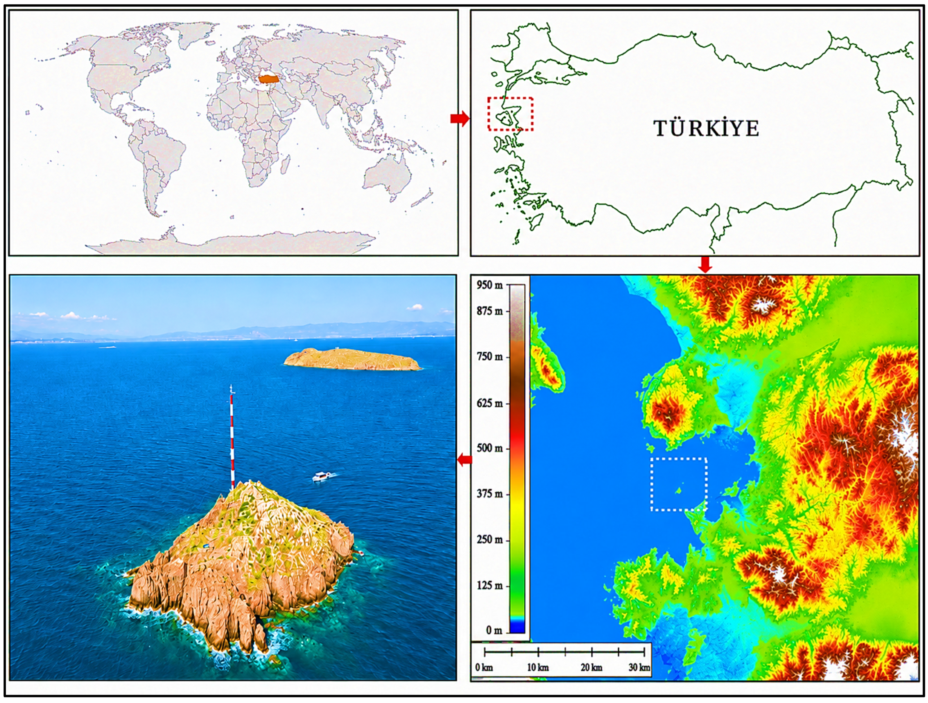
Figure 1. Geographic context and offshore measurement setting of the study area: global location of Türkiye shown in the upper left panel; national-scale location of the Northern Aegean study region within western Türkiye shown in the upper right panel; aerial view of Küçük Ada and the offshore meteorological mast shown in the lower left panel; and regional topographic map showing the Aliağa coastal zone and the offshore project area shown in the lower right panel. The arrows indicate the successive spatial zoom from the global scale to the local measurement site. The color-dashed line box represents the area where the wind measurement station is located.
Wind 06 00051 g001
Figure 2. Schematic spatial representation of the offshore meteorological mast location, surrounding ERA5 grid points, and the potential offshore wind farm area in the Northern Aegean study region. The blue-shaded marine area represents Turkish territorial waters, whereas the unshaded marine area on the western side denotes the maritime area outside Turkish territorial waters. The purple dot indicates the offshore meteorological mast location, while the red dots labeled A–D denote the four ERA5 grid points used in the long-term atmospheric analysis. The yellow-framed area represents the candidate offshore wind farm area considered during the site-selection and layout-evaluation process.
Wind 06 00051 g002
Figure 3. Response-specific machine-learning MCP workflow linking the concurrent 100 m observations, multi-grid ERA5 predictor construction, controlled algorithm comparison, selected Random Forest models, TreeSHAP interpretation and long-term 100 m reconstruction. Wind-speed magnitude was predicted directly, whereas wind direction was reconstructed from separately predicted zonal and meridional components.
Wind 06 00051 g003
Figure 4. Horizontal and vertical computational mesh structures of the project area: (left) horizontal mesh and (right) vertical mesh.
Wind 06 00051 g004
Figure 5. Wind measurement mast configuration.
Wind 06 00051 g005
Figure 6. Annual wind rose constructed from concurrent in situ measurements using wind speed at 41 m (WS1) and wind direction at 37 m (WD1). Colours indicate wind-speed classes, while the radial axis represents the frequency of occurrence for each directional sector.
Wind 06 00051 g006
Figure 7. Wind rose distributions derived from ERA5 wind data at 100 m for the four surrounding grid points A–D and from concurrent in situ measurements using wind speed at 41 m and wind direction at 37 m. The figure is intended to illustrate the directional consistency and spatial variability of the ERA5 wind field around the offshore mast location rather than a single interpolated point-to-point comparison. Colours represent wind-speed classes and radial distances indicate directional occurrence frequencies.
Wind 06 00051 g007
Figure 8. Wind rose of the reconstructed 21– year wind climate at 100 m.
Wind 06 00051 g008
Figure 9. Global TreeSHAP importance for the selected response-specific H2O Distributed Random Forest MCP models. Bars show mean absolute SHAP contributions over the concurrent measurement–ERA5 period. Panels correspond to scalar 100 m wind speed, the 100 m zonal component and the 100 m meridional component.
Wind 06 00051 g009
Figure 10. Wake-interaction indicator estimated using WindSim Wake Model 3 across the optimized wind farm layout under the dominant NE–E offshore wind regime. This figure provides a layout-scale qualitative visualization of the expected wake-affected zones and turbine-to-turbine interaction patterns. It should be interpreted as a wake-footprint indicator rather than a quantitative hub-height wind speed deficit map. Blue circles indicate wind turbine locations, while the purple circle denotes the offshore meteorological mast.
Wind 06 00051 g010
Figure 11. Quantitative wake-induced wind speed deficit distribution (m/s) at the 170 m hub-height level estimated using WindSim Wake Model 3 over the CFD-derived ambient wind field. The colour scale represents the magnitude of the local wind speed reduction: yellow tones indicate relatively weak to moderate wake-induced deficits, whereas the small orange-to-red regions immediately downstream of turbine locations indicate localized areas of stronger wind speed reduction. Blue circles indicate wind turbine locations, while the purple circle denotes the offshore meteorological mast.
Wind 06 00051 g011
Figure 12. Mean wind speed distribution (m/s) at hub height across the study area. Blue circles indicate wind turbine locations, while the purple circle denotes the offshore meteorological mast. The area enclosed by white dashed lines represents the overall area of the project.
Wind 06 00051 g012
Table 1. Wind measurement campaign summary.
DeviceParameterAveraging
Interval
Device ModelHeight (m)UnitMeanRecovery Rate
WS1 (Adolf Thies GmbH & Co. KG, Göttingen, Germany)Wind Speed10 minThies First Class Adv. II41m/s8.06695.25%
WS2 (Adolf Thies GmbH & Co. KG, Göttingen, Germany)Wind Speed10 minThies First Class Adv. II37m/s7.99595.25%
WS3 (Adolf Thies GmbH & Co. KG, Göttingen, Germany)Wind Speed10 minThies First Class Adv. II26m/s7.89595.25%
WS4 (Adolf Thies GmbH & Co. KG, Göttingen, Germany)Wind Speed10 minThies Clima15m/s7.66484.21%
WD1 (Adolf Thies GmbH & Co. KG, Göttingen, Germany)Wind Direction10 minThies First Class37DegNE95.25%
WD2 (Adolf Thies GmbH & Co. KG, Göttingen, Germany)Wind Direction10 minThies Clima15DegNE84.21%
Temp/RH (Adolf Thies GmbH & Co. KG, Göttingen, Germany)Temperature10 minGalltec Mela10°C18.90895.25%
Temp/RH (Adolf Thies GmbH & Co. KG, Göttingen, Germany) Humidity10 minGalltec Mela10%63.16695.25%
Pressure (R. M. Young Company, Traverse City, MI, USA)Air Pressure10 minRM Young10hPa1012.695.25%
Data Logger (Campbell Scientific, Inc., Logan, UT, USA)-10 minCampbell Scientific CR80010---
Table 2. ERA5 atmospheric variables available at grid points A, B, C and D.
ERA5 ParameterUnitERA5 ParameterUnit
100 m u-component of windm/sU-component of wind-850 hPam/s
100 m v-component of windm/sV-component of wind-850 hPam/s
10 m u-component of windm/sU-component of wind-700 hPam/s
10 m v-component of windm/sV-component of wind-700 hPam/s
2 m TemperatureKU-component of wind-500 hPam/s
2 m Dewpoint TemperatureKV-component of wind-500 hPam/s
Surface PressurePaU-component of wind-300 hPam/s
Mean sea level pressurePaV-component of wind-300 hPam/s
Boundary-layer heightmTemperature-850 hPaK
Surface latent heat fluxJ/m2Temperature-700 hPaK
Surface sensible heat fluxJ/m2Temperature-500 hPaK
Total cloud cover (dimensionless)(0–1)Temperature-300 hPaK
Surface solar radiation downwardsJ/m2Geopotential-850 hPam2/s2
Surface net thermal radiationJ/m2Geopotential-700 hPam2/s2
Table 3. Response-specific ML-MCP architecture and selected DRF configurations.
ResponseObservational ResponseEffective TreesReconstructed Output
ws100_obs100 m scalar wind-speed magnitude168Long-term 100 m wind-speed magnitude
u100_obs100 m zonal wind component166Long-term 100 m zonal component
v100_obs100 m meridional wind component171Long-term 100 m meridional component; direction reconstructed jointly from u/v
Table 4. Performance evaluation of machine learning models for offshore wind variable prediction.
TargetModelRMSEMAEBIASOOF Pearson r
u100_obsDRF2.2691.5880.0820.919
u100_obsGBM2.2771.5960.1550.919
u100_obsXGBoost2.3461.6540.2180.914
u100_obsDeep Learning2.4701.7740.1340.903
u100_obsGLM2.6611.9610.2880.891
u100_obsLinear Regression3.0002.2630.4060.854
v100_obsDRF2.4781.7890.0720.890
v100_obsGBM2.5421.8440.0810.883
v100_obsXGBoost2.5631.8860.1960.885
v100_obsDeep Learning2.7252.0360.2720.868
v100_obsGLM2.7372.0430.4120.872
v100_obsLinear Regression3.3822.6280.5130.794
ws100_obsDRF1.9691.504−0.0270.884
ws100_obsGBM1.9871.516−0.0380.873
ws100_obsXGBoost2.0661.5890.1190.882
ws100_obsDeep Learning2.1411.6220.1310.861
ws100_obsGLM2.1511.6800.2180.868
Table 5. Energy analysis summary features.
FeatureResult
Turbine ModelIEA284–22.0 MW
Hub Height (m)170
Number of Turbines65
Installed Capacity (MW)1430
Gross AEP (GWh/year)5794.8
Average Wind Speed (m/s)8.3
Wake Losses (%)5.2
Wake-Adjusted AEP (GWh/year)5494.5
Equivalent Full-Load Hours (h/year)3842.3
Capacity Factor (%)43.9
Disclaimer/Publisher’s Note: The statements, opinions and data contained in all publications are solely those of the individual author(s) and contributor(s) and not of MDPI and/or the editor(s). MDPI and/or the editor(s) disclaim responsibility for any injury to people or property resulting from any ideas, methods, instructions or products referred to in the content.