A Comparison of ASCE/SEI 7–22 Tornado-Induced Load Provisions for Residential Low-Rise Buildings to Those Evaluated Using Physical Simulation

Abstract

In this study, the loads induced by tornado-like vortices on scaled models of eight low-rise residential buildings with real-world shapes in a typical North American community are quantified and compared to the provisions provided by ASCE/SEI 7–22. Physical simulations of the interaction between translating tornado-like vortices representative of EF1-, EF2- and EF3-rated tornadoes and the scaled models were performed in the WindEEE Dome at the University of Western Ontario. Three internal pressure scenarios were numerically simulated. The tornado velocity gust factor was identified as a critical parameter when translating loads from the model to full-scale. The uplift forces on the whole roof in the internal pressure scenarios with one dominant opening are between 44% and 63% higher than the distributed leakage scenario, highlighting the importance of keeping the integrity of the envelope. Revised values of the internal pressure coefficients and external pressure coefficients or correction factors may be used to improve the ability of the standard to provide safer design loads.

1. Introduction

Tornado wind loads were not specified in building codes for a long time despite generating extensive damage and loss of life in many parts of the world [1], notably in the United States of America (USA), where they cause roughly twice as much loss as earthquakes and half as much as hurricanes [2]. Moreover, tornadoes cause the highest average loss per wind catastrophe in the Canadian provinces of Ontario and Quebec [3]. This omission was justified in ASCE/SEI 7–16 by the low probability of occurrence of tornadoes [4]; however, the latest edition of the standard (ASCE/SEI 7–22) states that “recent research on tornado climatology has shown that tornadoes occur with much greater frequency and intensity than had previously been quantified”, which is the reason for the addition of a full chapter on tornado-resistant design in ASCE/SEI 7–22 [5].

In additional to the evidence that tornadoes occur more frequently than thought, a careful analysis of tornado damage records and the associated wind levels has indicated that most tornado damage is induced by tornadoes rated 3 or lower in the Enhanced Fujita (EF) Scale [2]. Furthermore, EF ratings are assigned according to the maximum velocity inferred from the Degrees Of Damage (DOD) observed in Damage Indicators (DIs), which means that most of the damaged area is caused by lower-intensity winds. For example, the Tuscaloosa (2011) tornado rated EF4 had only 2.7% of the damaged area rated as EF4; the other 97.3% was EF0-EF3 damage [6]. The wind speed associated with EF0-EF3 is comparable to hurricane winds for which ASCE/SEI 7 has had provisions for decades and mitigation measures have been implemented. These observations led van de Lindt et al. [7] to propose a dual-objective-based approach to design for tornadoes that considers reducing damage for tornadoes rated EF3 or lower and minimizing the loss of life for high-end EF4- or EF5-rated tornadoes.

The current understanding of tornado-induced loads is limited when compared to Atmospheric Boundary Layer (ABL)-induced loads for which the conventional ABL wind tunnel technique is mature. The recent relative proliferation of Tornado Vortex Generators (TVGs) designed for wind engineering applications [8,9,10,11,12,13,14] has allowed for a better comprehension of tornado-induced loads and some quantitative knowledge.

The loading effect of tornado-like vortices (TLVs) on low-rise buildings has been investigated by several researchers employing physical simulation [15,16,17,18,19,20,21,22,23,24,25,26,27,28,29,30,31]. There is considerable agreement that the pressure distribution patterns induced on the surface of low-rise buildings by tornadoes and straight-line winds are different. This difference is caused by the three-dimensional nature and curvature of the flow in tornadoes. The reported values of the tornado-induced to straight-line-induced pressure coefficient ratios are significantly scattered.

Most past studies have focused on isolated buildings. Only a few have considered the effect of multiple buildings and their sheltering effect, e.g., Zhang and Sarkar [10] and Sabareesh et al. [25]. They concluded that lateral forces can be reduced by the presence of adjacent buildings but the uplift force can decrease or increase without a clear pattern. Case et al. [21] analyzed the effect of low-rise building geometry on tornado-induced loads and found that the loads depend on “eave height, roof pitch, aspect ratio, plan area, and other differences in geometry such as the addition of a garage and modeling of the roof overhang and soffit”. No study has analyzed the loading on residential low-rise buildings with complex roof configurations and plan shapes. All studies have considered simple gable roof buildings.

Tornadoes induce a pressure deficit around their core that has no counterpart in straight-line winds. This depression, usually termed Atmospheric Pressure Deficit (APD) [26], develops as the flow needs a radial pressure gradient to balance centrifugal forces. The building’s internal pressure behavior depends on the APD, the capacity of the building to respond to atmospheric pressure changes and the presence of large openings in the envelope. Therefore, measuring or modelling internal pressure is critical, even more so than in ABL flows. Some researchers have included an internal pressure model [26] or direct measurements [28] in their evaluation of tornadic loads. For straight-line winds, it has been established that the use of Multiple Discharge Equations (MDEs) can lead to accurate estimates of the internal pressure time series based on external pressures, even capturing the Helmholtz resonant peak [32]. The effectiveness of this model in predicting internal pressure under tornado winds was evaluated by Jaffe and Kopp [33]. They found that the MDE model reasonably reproduces internal pressures but with lower accuracy than under straight-line winds, which can be explained by the presence of sub-vortices and the vertical component of the wind velocity.

In December 2021, an updated ASCE/SEI 7–22 Minimum Design Loads and Associated Criteria for Buildings and Other Structures was released. This standard included a chapter (Chapter 32) on tornado-resistant design for buildings in Risk Categories III and IV in tornado-prone areas [5]. This is the first standard to include provisions for tornado-induced loads. ASCE/SEI 7–16 [4] provided design guidance for tornadoes to reduce damage caused by EF0- to EF2-rated tornadoes or increase occupant protection, but it was not mandatory. The guidance from ASCE/SEI 7–16 was only for owners who wanted to have a higher level of safety on their property even knowing that designing for tornadoes implies a much higher design return period than typically used for residential buildings.

The procedures outlined in Chapter 32 of ASCE/SEI 7–22 for calculating tornado provisions follow the same fundamental logic as the chapters addressing straight-line wind loads. This approach aims to maintain simplicity and encourage widespread adoption. However, there are notable differences that are worth mentioning. These include the following:

• The tornado design wind speed is the expected tornado velocity with 1700- and 3000-year return periods for Risk Categories III and IV, respectively, which depend on the plan area of the building. Tornado design wind maps are provided for the estimation of the design wind speed.
• The directionality factor depends on the structure type.
• The exposure coefficient in Chapter 32 decreases with height.
• The enclosure classification is performed considering each wall as a windward wall.
• If the glazed openings are not required to be protected, the building shall be evaluated as a partially enclosed building in Chapter 32.
• A new sealed enclosure classification is incorporated for which the internal pressure coefficient is +1.0.
• An external pressure coefficient adjustment factor for vertical winds ($K_{vT}$) is introduced. This factor corrects the pressure coefficients obtained from Chapters 27 and 30 in ASCE/SEI 7–22, for the increased vertical angle of attack.

The tornado load calculations in ASCE/SEI 7–22 involve utilizing pressure coefficients obtained from ABL wind tunnel tests. These coefficients are subsequently adjusted by the factor $K_{vT}$ to accommodate variations in the vertical angle of attack. While this approach has contributed to the progress of the standard, it poses challenges and may potentially introduce significant errors, as indicated by the evidence summarized in the preceding paragraphs.

The scope of Chapter 32 of ASCE/SEI 7–22 is limited to buildings in Risk Category III or IV located in tornado-prone areas; therefore, residential low-rise buildings are excluded. Despite this, its publication presents a good opportunity to evaluate the performance of residential low-rise buildings designed following its provisions.

This research aims to quantify the expected maximum loads on residential low-rise buildings subjected to tornado loading and compare them to the design loads provided by ASCE/SEI 7–22 for tornadoes. For this, the loads induced by several translating TLVs generated in the WindEEE Dome at the University of Western Ontario (UWO) on a model of a part of the community of Dunrobin, Ontario, Canada, which was affected by a tornado in September 2018, are compared to ASCE/SEI 7–22 provisions. The TLVs used here have been shown to match the characteristics of some real tornadoes ranging from EF1 to low-end EF3. The model includes eight low-rise residential buildings with different real-world roof geometries, i.e., gable, hip, hip and valley, and dormer roofs representing a typical North American wood-frame residential community. Different scenarios in terms of internal pressure are simulated using the MDE model.

2. Experimental Setup

2.1. Physical Simulations

The physical simulations presented in this research were performed at the Wind Engineering, Energy, and Environment (WindEEE) Dome at the UWO, Canada. The WindEEE Dome is a novel wind testing chamber capable of modeling a wide range of three-dimensional and time-dependent atmospheric flows, focused on wind engineering, wind energy, and environmental problems, as its name implies. Specifically, the facility aims to reproduce tornadoes, downbursts, gusts, currents, shear flows, and boundary layer flow at high Reynolds numbers [34].

The main chamber is hexagonal with a diameter of 25 m. This chamber is surrounded by a hexagonal return chamber 40 m in diameter. On the periphery of the main chamber, there are 100, 30 kW fans, of which 60 are located on one lateral wall in a 4-row by 15-column arrangement. On the ceiling, a mobile bell mouth communicates between the main chamber and the upper plenum, where 6, 220 kW fans can generate flow into or out of the main chamber. The mobile bell mouth allows for the simulation of translating TLVs and downbursts. A section of the facility is shown in Figure 1.

There are two modes of operation to produce TLVs: Modes A and B. In Mode A, only the upper plenum fans operate in suction mode. At the same time, the circulation is created by inducing a tangential component to the returning flow using directional louvers [35]. The scale of the TLVs is enhanced in Mode B operation by activating the peripheral fans [36].

2.2. The Wind Flow

The flow characteristics in TLVs are controlled by the swirl ratio

$$\begin{array}{c}\mathrm{S}={\displaystyle \frac{r_0{\Gamma }_{\infty }}{2Q}},\hfill \end{array}$$

(1)

the aspect ratio a and only weakly by the Reynolds number [37]. In Equation (1), Q is the incoming flow rate, $r_0$ is the radius of the convergence zone and ${\Gamma }_{\infty }$ is the background circulation. The aspect ratio is defined as $a=h/r_0$, where h is the inflow depth. The swirl ratio is a measure of the relative spin of the tornado to the radial velocity. It has been shown that the structure of TLVs changes as the swirl ratio increases, from a single laminar vortex ($\mathrm{S}<0.2$), to a single vortex with breakdown ($0.2<\mathrm{S}<0.4$), then to two interlocking spiral vortices ($0.4<\mathrm{S}<1.0$), and finally, the two-celled vortex undergoes a transition to multiple vortices revolving about a common center ($\mathrm{S}>1.0$) [38,39].

All TLVs in this research were generated using Mode A. The flow characteristics of these TLVs were investigated by Refan and Hangan [35]. The reader is referred to the cited article for flow details. A summary of the most important average parameters of the TLVs generated in Mode A is presented in

Table 1. Characteristics of the TLVs generated in Mode A.

$\mathbf{S}$	${\mathit{V}}_{\mathit{tan},\mathit{max}}$ (m/s)	${\mathit{r}}_{\mathit{c},\mathit{max}}$ (m)	${\mathit{z}}_{\mathit{max}}$ (m)	EF-Rating	${\mathit{\lambda }}_{\mathit{L}}$	${\mathit{\lambda }}_{\mathit{V}}$
0.21	8.8	0.27	0.2	-	-	-
0.48	11.5	0.45	0.2	EF1	160–300	-
0.59	12.8	0.42	0.2	-	-	-
0.76	13.8	0.60	0.2	EF2	200–280	∼2.1
1.03	16.2	0.69	0.2	EF3	200–280	∼2.1

. In Table 1, $V_{tan,max}$ is the average maximum tangential wind speed, $r_{c,max}$ is the radius to the maximum tangential wind speed, $z_{max}$ is the vertical location of the same wind speed, ${\lambda }_L$ is the geometric scale, ${\lambda }_V$ is the velocity scale, and EF-rating is the equivalent rating, as explained next. The length and velocity scales were estimated only for some TLVs. The inflow depth is fixed at $h=0.8$ m.

Refan et al. [40] developed a methodology to match the flow in real tornadoes and TLVs. They found a weak relationship between the swirl ratio and the EF-rating for a limited set of real tornadoes and the TLVs simulated in a small vortex chamber, a 1:11 scaled replica of the WindEEE Dome. Using the same technique, Refan and Hangan [35] matched the flow of some tornadoes to the flow in TLVs simulated in the WindEEE Dome using Mode A. They were able to identify swirl ratio ranges for different EF-rated tornadoes. Based on this work, here we use the flow of TLVs with swirl ratios $\mathrm{S}=0.48$, $0.76$, and $1.03$ as representative of tornadoes rated EF1, EF2, and EF3, respectively. From now on, EF-rating and swirl ratio are used interchangeably; however, the reader needs to remember that this equivalence is only valid in the context of this research. Therefore, the conclusions in this work need to be taken carefully since they may not be extended to all tornadoes in the EF1 to EF3 range.

In addition, it is important to note that the characteristics of TLVs were studied for the stationary case; therefore, for the translating case, it is assumed that the characteristics are unchanged for the same hardware set-up. A similar approach was also adopted by Romanic et al. [41].

2.3. Model and Measurements

As mentioned before, a neighborhood in Dunrobin, Ontario that was affected by the passage of the 21 September 2018, EF3-rated tornado was used as an example of a typical North American residential community. The scaled model of the community consists of eight instrumented residential low-rise buildings with twenty-two non-instrumented surrounding buildings at a 1:150 geometric scale (see Figure 2b). This geometric scale was selected as a compromise between the need for the buildings to be large enough to fit a considerable number of pressure taps and the TLVs’ length scale presented in Table 1. The model scale is slightly higher than the TLVs scale. The instrumented houses are located inside the near rectangular shape delimited by the roads in Figure 2a. The scaled models were 3D-printed at UWO’s Machine Services (UMS). The total number of pressure taps was 1152, distributed on the surface of the eight instrumented houses and the ground plate. Each house had an average of 140 pressure taps.

The pressure measurement system consists of miniature Electronic Pressure Scanners (EPSs) coupled with Digital Temperature Compensation (DTC) Initiums. The pressure scanners used in this study are ESP-32HD, originally manufactured by Pressure Systems, Inc. (PSI), which have 32 scanning ports each. These scanners are now produced and sold by TE Connectivity (Berwyn, PA, USA) following PSI’s integration into the company. ESP Pressure Scanners are miniature electronic differential pressure measurement units consisting of an array of silicon piezoresistive pressure sensors, one for each pressure port. This device allows for measurement at frequencies up to 70,000 Hz per channel. The scanner’s amplified analog output is then sampled at a remote A/D converter (DTC Initium). The DTC Initium is connected to the scanner via an Ethernet-based connection. The accuracy of the DTC Initium is $\pm 0.05\%$ over the entire operating temperature range (0 °C–70 °C). The scanners are connected to the pressure taps using a tubing system that acts like a low-pass filter attenuating the signal at frequencies higher than 210 Hz, the cut-off frequency of the filter. To eliminate aliasing from the pressure signal, the sampling frequency is set at 500 Hz, higher than two times the cut-off frequency of the low-pass filter (Nyquist rate).

The wind velocity measurements were performed using a vertical array of four Cobra Probes from Turbulent Flow Instrumentation Pty Ltd. (TFI) at heights 2, 5, 10, and 20 cm. The system of cobra probes, located one radius of maximum wind (RMW) away from the path of the simulated tornado, was synchronized to the pressure measurement system. The four-hole differential pressure Cobra Probes can measure the three components of the velocity and local pressure at frequencies lower than 2000 Hz. These probes can correctly resolve the components of the wind velocity only when the angle between the wind velocity vector and the probe x-axis is less than 45°. The analog output is then read by an A/D converter. The velocity components are calculated using proprietary acquisition software. The manufacturer claims that the Cobra Probes need no additional calibration other than the factory calibration.

Table 2. Parameters of the studied cases.

Case Code	S	Offset	Angle	Movement	Number of Runs	Sampling Time (s)
W3E1	1.03	0	80	Translation	9	60
W3E2	1.03	0	45	Translation	5	60
W3E3	0.76	0	45	Translation	5	60
W3E4	0.76	0	80	Translation	5	60
W3E5	0.48	0	80	Translation	5	60
W3E6	0.48	0	45	Translation	5	60
W3E7	0.48	+RMW	45	Translation	5	60
W3E8	0.48	+RMW	80	Translation	5	60
W3E9	0.76	+RMW	80	Translation	5	60
W3E10	0.76	+RMW	45	Translation	5	60
W3E11	1.03	+RMW	45	Translation	5	60
W3E12	1.03	+RMW	80	Translation	5	60
W3E13	1.03	0	-	Stationary	1	120
W3E14	0.76	0	-	Stationary	1	120
W3E15	0.48	0	-	Stationary	1	120
W3E16	1.03	+2RMW	80	Translation	5	60
W3E17	1.03	+2RMW	45	Translation	5	60

shows the parameters of the 17 different configurations tested. Three cases (W3E13, W3E14, and W3E15) involve stationary TLVs with $\mathrm{S}=0.48$, $\mathrm{S}=0.76$, and $\mathrm{S}=1.03$, which are centered on the model table (see Figure 3). In the other 14 cases, the TLVs translate along a quasi-straight line path. Two translating directions were selected: (1) 80° from north clockwise, which represents the actual path of the 2018 Dunrobin tornado, and (2) 45°, which is the most probable orientation for strong tornadoes [42]. For each direction, TLVs with $S=0.48$, $S=0.76$, and $S=1.03$ were simulated with two offsets from the center: (1) zero and (2) one RMW. Two more translating TLVs with $S=1.03$ were simulated at both mentioned translating directions with an offset of 2 RMW to consider the uncertainty of the actual location of the Dunrobin tornado path. Figure 3 shows the paths of the translating TLVs. The central path (orange) in both sub-figures is shared by the TLVs with the three swirl ratios considered.

The translation speed of all TLVs was fixed at $1.3\mathrm{m}/\mathrm{s}$. Thus, the ratio between translation and tangential velocity falls between 0.08 and 0.11. For comparison, the Dunrobin tornado parent cloud speed was close to 70 kmh; therefore, the ratio between translation and tangential velocity was around 0.3. Hence, this value represents a relatively slow-moving tornado. The case with $S=1.03$ and zero offsets was repeated nine times. All other translating TLVs were repeated five times. The sampling time for translating TLVs was 60 s and 120 s for the stationary TLVs. However, note that the actual movement period is much shorter than the sampling time. During most of the sampling time, the TLVs are stationary in the initial and final position.

3. Procedure

The applicability of the procedures in ASCE/SEI 7–22 is restricted to “regular shape” buildings. The definition of regular shape given in the standard is as follows: “A building or other structure that has no unusual geometrical irregularity in spatial form”, and it adds examples of irregular buildings: “buildings with multiple setbacks, curved facades, or irregular plans resulting from significant indentations or projections, openings through the building, or multitower buildings connected by bridges”. Most residential low-rise buildings do not fit exactly into this definition. It is common to see L, T, and other plan shapes, hip and valley, dormer, cross-hipped, intersecting roofs, and more. Despite this, the standard recognizes the practical necessity to balance the range of applicability between situations that are outside but reasonably close to the “regular shape” building archetype, while restricting the use of clearly unusual shapes that need wind tunnel testing. In addition, it is expected that the loads calculated using the pressure coefficients obtained from the simple archetypes of the standard to be conservative when applied to complicated shapes [4]. Accordingly, it is assumed that the provisions can be applied to the Dunrobin model houses.

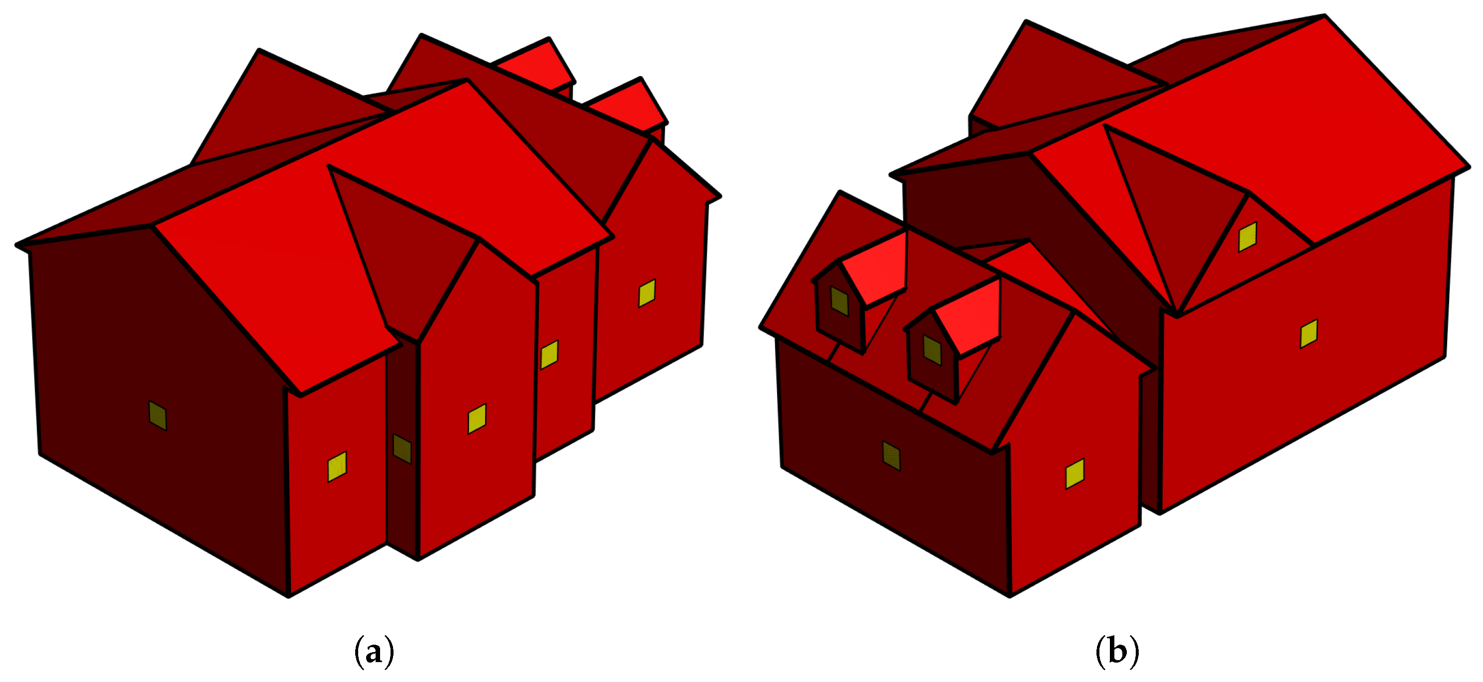
The gable roof archetypes in ASCE/SEI 7–22 look like the one depicted in Figure 4a. For the Components and Cladding (C&C) pressure comparison, only the part of the building that has a gable roof is considered. This can be better understood by observing Figure 5a, which shows, in color, the part of the building used for the calculation of C&C pressure coefficients; the grey part is ignored.

The pressure coefficients given in ASCE/SEI 7–22 for the calculation of forces for the Main Wind Force Resisting System (MWFRS) in enclosed buildings are limited to very simplified shapes, i.e., simple gable roofs, simple mansard roofs, and simple mono slope roofs. The practitioner who must deal with the calculation of forces for design in typical residential buildings, like the ones in the Dunrobin community using the standard, will have to make some assumptions in order to estimate the loads. For the calculation of overall forces, we use a virtual “envelope” gable roof house created from the outline of each building. This envelope building will have more frontal area and roof area than the actual building; therefore, the loads are likely to be higher than the actual loads experienced by the building. The uplift force on this virtual house is multiplied by the ratio of the actual plan area of the house to that of the virtual house. The concept of the envelope house is shown in Figure 5b for House 1. Dormers are ignored.

We decided to remove the hip roof building (House 3) in this analysis for two reasons. (1) There is only one building with this type of roof, which limits the generality of any conclusion we could draw from it, and (2) it would add a large number of different zones, which would make the results unmanageable and difficult to follow for the reader.

For the MWFRS calculations, the pressure coefficients are extracted from Chapter 27, Figure 27.3-1 in ASCE/SEI 7–22. For C&C, the pressure coefficients are obtained from Chapter 30, Figure 30.3-1 and Figures 30.3-2C. Figure 4b shows the C&C zones 1 (blue), 2 (red), 3 (yellow), 4 (green), and 5 (orange), in ASCE/SEI 7–22.

Since the pressure tap density is not high enough to allow for area-averaged pressure coefficient calculation around areas close to 10 ${\mathrm{ft}}^2$ in full-scale, the comparison is performed for point pressure. This means that the pressure measured is not spatially averaged and the pressure coefficients for the code calculations are found from the horizontal part of the plots in Figures 30.3-1 and 30.3-2C in ASCE/SEI 7–22 at effective wind areas (EWAs) lower than 10 ${\mathrm{ft}}^2$.

3.1. ASCE/SEI 7–22 Design Provisions

The pressure calculation for tornado-induced load provisions for MWFRS is performed in accordance with the following equations:

$$\begin{array}{c}p=q{G}_T{K}_{dT}{K}_{vT}{C}_p-q_i\left(G{C_p}_{iT}\right)\hfill \end{array}$$

(2)

$$\begin{array}{c}q=0.613K_{zT}{K}_e{V}_T^2\left(Pa\right)\hfill \end{array}$$

(3)

where $q_i=q$, and the directionality factor for tornadoes $K_{dT}=0.8$, while the tornado exposure coefficient $K_{zT}=1.0$ and the ground elevation factor $K_e=1.0$. The gust-effect factor for tornadoes is $G_T=0.85$, $V_T$ is the design tornado wind speed, the external pressure coefficient adjustment factor for vertical winds is $K_{vT}=1.1$ and, as usual, $C_p$ is the external pressure coefficient and ${G{C}_p}_{iT}$ is the tornado internal pressure coefficient, which is +1.0 for sealed classification and +0.55 for the enclosed and partially enclosed classification.

For C&C, the equations used are:

$$\begin{array}{c}p=q_{hT}\left[K_{dT}{K}_{vT}\left(G{C}_p\right)-\left(G{C_p}_i\right)\right]\hfill \end{array}$$

(4)

and Equation (3) with $q_{hT}=q$. Now, $K_{dT}=0.75$, the external pressure coefficient adjustment factor for vertical winds is $K_{vT}=1.2$ for Zone 1, $K_{vT}=1.2$ for Zone 2 and $K_{vT}=1.3$ for Zone 3.

It is important to note that for ASCE/SEI 7–22, the design wind speed is determined from maps. These maps depend on the risk category of the building and the plan area of the structure. Here, the end-of-range of the EF-rating considered is used as $V_T$ for consistency.

3.2. Physical Simulation Calculations

The forces on any part of each model house can be calculated by adding the contributions of each pressure tap on the surface of the building using Equation (5).

$$\begin{array}{c}{\mathbf{F}}_M\left(t\right)=-\sum _{j=1}^N\left[p_j\left(t\right)-p_{int}\left(t\right)\right]A_j{\mathbf{n}}_j\hfill \end{array}$$

(5)

where the subscript M indicates force on the model, j is the identification number of the pressure taps from 1 to N, which is the total number of pressure taps that are involved in the calculation of the force, $p_j\left(t\right)$ is the time history of the pressure on tap j, $p_{int}\left(t\right)$ is the time history of the internal pressure for the house being considered, $A_j$ is the tributary area assigned to tap j and ${\mathbf{n}}_j$ is the unit normal vector for each pressure tap. Equation Equation (5) defines the uplift force on the roof as positive and the downward force as negative.

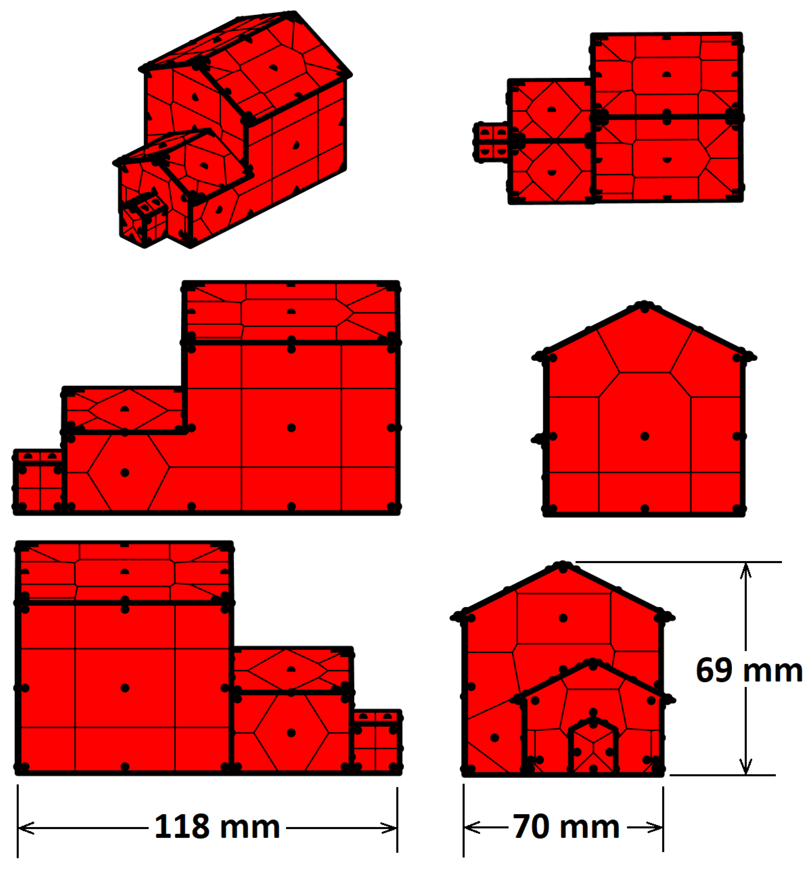
On each face, the tributary areas assigned to each pressure tap $A_j$ are defined using Voronoi polygons [43]. In Appendix A, Figure A1–Figure A7 show the geometries of the model buildings and the position of the pressure taps on all houses along with the tributary areas assigned to each pressure tap. It is important to note that in some cases, the tributary areas are quite large due to the complexity and size of the model buildings. However, because the overall force is calculated by summing the contributions from each tributary area, the impact of localized peak pressures is expected to be mitigated.

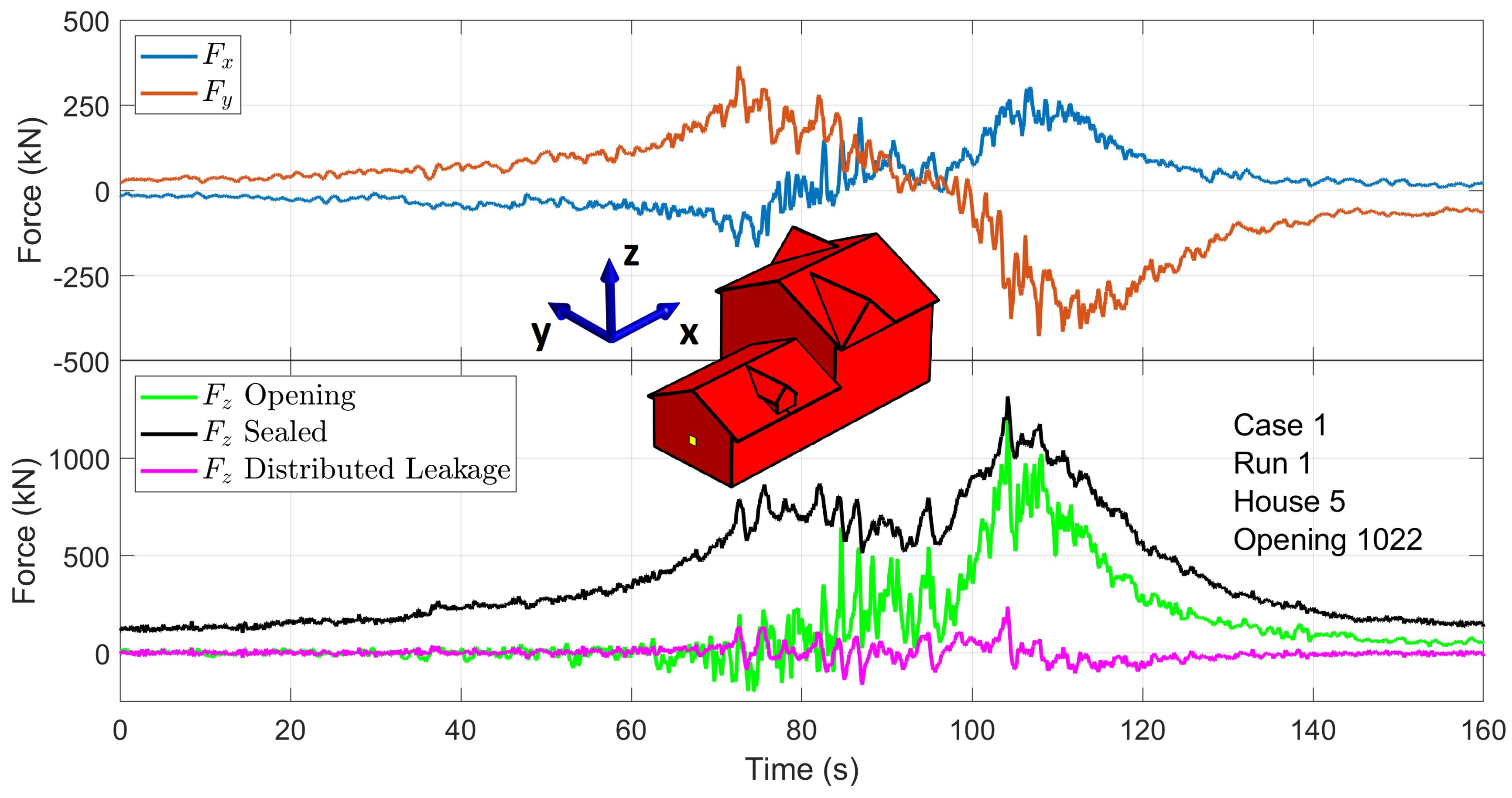
As an example, Figure 6 shows the time histories of the overall lateral force components on House 5 in Case 1, Run 1, and the uplift force on the roof with a dominant opening (yellow square), with distributed leakage and sealed internal pressure scenarios in full-scale. These scenarios are explained in Section 3.4.

For each case, the set of peak forces or pressures is obtained from each run and fitted to a type-I Generalized Extreme Value Distribution (GEVD) using Lieblein’s BLUE method [44,45] to calculate the nominal extreme force or pressure. The nominal extremes are computed as the 78th percentile of the distribution. The decision to use the 78th percentile as the nominal extreme value was made in line with the common practice [46]. However, it needs to be noted that the 78th value was obtained by Cook and Mayne [47] for ABL flow climate in the UK by convolution of the extreme value distributions of the wind speed and the pressure coefficient for a target probability of exceedance [48]. A similar analysis for tornadoes is out of the scope of this research and, therefore, was not performed. Nevertheless, since the design velocities used here are fixed for each EF-rating, if several tornadoes of the same intensity following a similar path hit one building, the loads would overcome the nominal extreme value 22% of the times. This value may seem high, however, since the values reported in the results section are the highest ratio between the nominal loads and the loads calculated by the code; the probability of the nominal loads being surpassed ia much lower. This effect can be explained if it is observed that the worst ratio is achieved for a particular tornado path and house; therefore, this worst condition is very unlikely to happen in the event of a tornado strike.

3.3. Velocity Scales

The full-scale pressures are calculated using dimensional analysis. Assuming equality of pressure coefficients at full-scale $\left({C_p}_{FS}\right)$ and model scale $\left({C_p}_{MS}\right)$ leads to

$$\begin{array}{cc}{\displaystyle \frac{p_{MS}-{p_{ref}}_{MS}}{p_{FS}-{p_{ref}}_{FS}}}\hfill & ={\lambda }_V^2\hfill \end{array}$$

(6)

where $p_{MS}$ and $p_{FS}$ are the pressure at the same building location in the model and full-scale, respectively, ${p_{ref}}_{MS}$ and ${p_{ref}}_{FS}$ are the reference pressure in the model and full-scale, respectively, and the velocity scale is

$$\begin{array}{c}{\lambda }_V={\displaystyle \frac{{V_{ref}}_{MS}}{{V_{ref}}_{FS}}}\hfill \end{array}$$

(7)

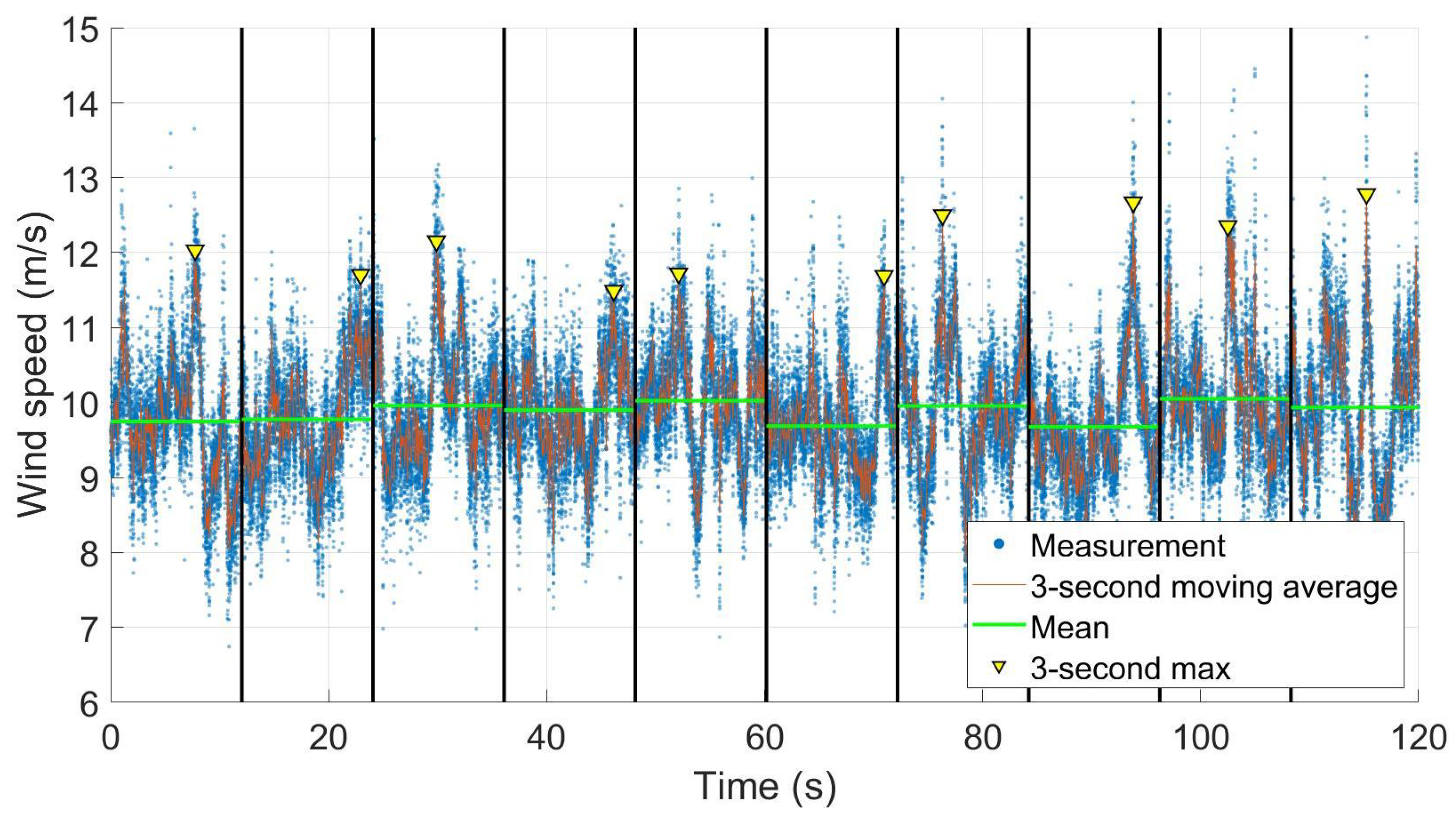
where ${V_{ref}}_{MS}$ and ${V_{ref}}_{FS}$ are reference velocities in the model and full-scale, respectively. Both reference velocity and pressure must be equivalent in the model and full-scale. This means that, if for instance, ${V_{ref}}_{FS}$ is a 3 s gust, then ${V_{ref}}_{MS}$ must also be an equivalent 3 s gust (3 s at model scale). The term “3-s gust” refers to the expected value of the 3 s moving average peak of the wind speed in full-scale.

In the same way, assuming equality of force coefficients in full-scale $\left({C_F}_{FS}\right)$ and in model scale $\left({C_F}_{MS}\right)$ leads to

$$\begin{array}{cc}{\displaystyle \frac{{\mathbf{F}}_{MS}}{{\mathbf{F}}_{FS}}}\hfill & ={\lambda }_V^2{\lambda }_L^2\hfill \end{array}$$

(8)

where ${\mathbf{F}}_{MS}$ and ${\mathbf{F}}_{FS}$ are forces in the model and full-scale, respectively. ${\lambda }_L$ is the length scale defined as the ratio of the model to full-scale reference lengths. The length scale is readily available from the geometric scale used for the model, that is, ${\lambda }_L=1/150$.

As explained before, ASCE/SEI 7–22 uses a 3 s gust design velocity with a return period that depends on the Risk Category of the structure, its plan area, and its location. On the other hand, the physically simulated TLVs are characterized by a maximum mean velocity, which is the maximum temporal average of the tangential velocity measured in a stationary condition. Since both reference velocities have different meanings, that is, in full-scale is a 3 s gust and in the model is a mean velocity, one of them must be transformed to find two equivalent reference velocities. For instance, the full-scale reference 3 s gust velocity has to be transformed to a mean velocity in full-scale or the model mean velocity has to be converted to an equivalent 3 s gust velocity at the model scale.

The transformations between mean and 3 s gust velocity make use of a tornado velocity gust factor $G_{vTor}$ defined as follows:

$$\begin{array}{c}{G}_{vTor}\left(t,T\right)=E\left[{\displaystyle \frac{\widehat{u}\left(t,T\right)}{\overline{\mathrm{U}}}}\right]\hfill \end{array}$$

(9)

where $\widehat{u}\left(t,T\right)$ is the peak value of the moving average velocity with a window width t in the period T, $\overline{\mathrm{U}}$ is the mean velocity for the period T, and $E\left[·\right]$ denotes expected value.

In the past, researchers have used a variety of values and methods to determine the gust factors for tornadoes. Wang and Cao [29] and Haan Jr et al. [19] used the Durst curve, which was derived for ABL flows, to obtain a gust factor. Haan Jr et al. [19] explained that the use of the Durst curve is not ideal, but at the time, there were no turbulence measurements within tornadoes or TLVs available which could have allowed for a more accurate determination. The value used by Wang and Cao [29], $G_{vTor}=1.57$, is the gust factor with a 1 s averaging window and T = 3600 s. The gust factor utilized by Haan Jr et al. [19], $G_{vTor}\approx 1.4$, was determined for a 3 s averaging window and a period equivalent at full-scale to the averaging time selected, which translated to between 310 s and 450 s in full-scale. Roueche et al. [26] used a different approach. Their reference velocity in the model scale was calculated as the average of the maxima of the 3 s equivalent moving average of the wind velocity time history measured using cobra probes. The 3 s equivalent window width was found using a fixed velocity scale.

This research proposes an iterative method for evaluating the velocity scale and velocity gust factor. In contrast to Roueche et al. [26], where the window is fixed, the 3 s averaging window width is selected to match the velocity scale in the proposed method. More specifically, the wind speed measurements of the stationary TLVs are utilized in the following way:

• A velocity gust factor $G_{vTor}$ is assumed. An initial $G_{vTor}=1.2$ was used here.
• With the velocity gust factor, a velocity scale can be calculated using:

  $$\begin{array}{c}{\lambda }_V={\displaystyle \frac{V_M{G}_{vTor}}{V_{FS}}}\hfill \end{array}$$

  (10)

  where $V_M$ is the average maximum tangential wind speed (Table 1) and $V_{FS}$ is the 3 s gust wind speed in the target tornado EF-rating, i.e., end-of-range speed for the EF rating being considered.
• A time scale is calculated as

  $$\begin{array}{c}{\lambda }_T={\displaystyle \frac{{\lambda }_L}{{\lambda }_V}}\hfill \end{array}$$

  (11)
• Then, the 3 s equivalent window width ($w_s$) in samples is found using

  $$\begin{array}{c}{w}_s=3·{\lambda }_T·f\hfill \end{array}$$

  (12)

  where $f=500\mathrm{Hz}$ is the sampling frequency. The window size equivalent to $w_s$, but in seconds, is denoted by $w_t$.
• Apply a moving average with window width $w_s$ to the measured velocity time history in the model scale.
• Divide the obtained 3 s equivalent time history into an appropriate number of segments. Here, the time history is divided into 10 segments with 6016 samples each. The number of segments is arbitrary but has an influence on the value of the gust factor obtained; therefore, it must be selected carefully. Figure 7 illustrates this process graphically for the EF3-rated TLV.
• For each segment, the maximum 3 s equivalent gust ($V_{3s,max,i}$) is found along with the average velocity ($V_{mean,i}$), where i denotes the i-th segment.
• The velocity gust factor is calculated as the average of the quotient between the maximum 3 s velocity and the average velocity, for the 10 segments:

  $$\begin{array}{c}{G}_{vTor}={\displaystyle \frac{1}{10}}\sum _{i=1}^{10}{\displaystyle \frac{V_{3s,max,i}}{V_{mean,i}}}\hfill \end{array}$$

  (13)
• If the difference between the calculated velocity gust factor and the one assumed in Step 1 is higher than a specified tolerance, we go back to Step 1 but using $G_{vTor}$ obtained in Step 8 and repeat Steps 1 to 9. If the difference is less than the selected tolerance, we stop the iteration.

This process converges in less than 10 iterations for a 0.001 tolerance, leading to the values presented in

Table 3. Scales and parameters of the TLVs scaled to EF end-of-range tornadoes.

Rating	Segment Length $\left(\mathit{s}\right)$	${\mathit{\lambda }}_{\mathit{V}}$	${\mathit{\lambda }}_{\mathit{T}}$	${\mathit{w}}_{\mathit{t}}\left(\mathit{s}\right)$	${\mathit{w}}_{\mathit{s}}\left(\mathit{samples}\right)$	${\mathit{G}}_{\mathit{vTor},\mathit{ref}}$
EF1	586	1:3.08	1:48.7	0.062	31	1.39
EF2	514	1:3.51	1:42.8	0.070	35	1.25
EF3	486	1:3.71	1:40.4	0.074	37	1.23

. We denote the values obtained using this procedure as the nominal velocity gust factors $G_{vTor,nom}$. Observe that the nominal velocity gust factor decreases as the equivalent rating increases. In WindEEE, the amplitude of the wandering movement of the TLVs, which is the random motion of the tornado center around a point, is higher relative to the size of the TLVs as the swirl ratio decreases [49]. Consequently, a fixed probe may record higher relative amplitude velocity fluctuations for lower than for higher swirl ratios, which may result in higher gust factors for low $\mathrm{S}$. Although tornado wandering may be present in nature, it has not been characterized; therefore, it is not known if the wandering of TLVs created inside WindEEE is representative of the actual tornado random movement.

In addition to the possible amplification of the gust factors induced by wandering at low swirl ratios, the method has other limitations. The velocity record was split into 10 segments that roughly correspond to 10 min duration tornadoes in full scale; this may not be appropriate for all tornado ratings. Moreover, the TLVs are scaled to EF end-of-range tornadoes, which may be inappropriate, specifically when ASCE/SEI 7–22 prescribes a design wind speed that varies according to location, plan area, and type of structure.

We define a nominal ratio $r_{nom}$ between the forces or pressures calculated from physical simulation (PS) using the gust factors shown in Table 3 and the equivalent loads calculated using the standards (CODE) in full scale, that is:

$$\begin{array}{cc}{r}_{F,nom}\hfill & ={\displaystyle \frac{F_{PS}}{F_{CODE}}}\hfill \end{array}$$

(14)

$$\begin{array}{cc}{r}_{p,nom}\hfill & ={\displaystyle \frac{p_{PS}}{p_{CODE}}}.\hfill \end{array}$$

(15)

It is evident that $F_{PS}$ and $p_{PS}$ depend on the value of the gust factor used to calculate the velocity scale (Equation (10)); therefore, the ratios depend on the value of the gust factor as

$$\begin{array}{c}r\propto G_{vTor}^{-2}.\hfill \end{array}$$

(16)

Considering all the uncertainties involved in the calculation of gust factors, and the fact that the ratios depend strongly on the velocity gust factor used, we provide the reader with a method to adjust the reported ratios if a different gust factor is preferred.

A high gust factor leads to low ratio values and vice versa. Different gust factors lead to different velocity scales, and therefore, the scaled internal volume of the building is affected (see discussion in Section 3.4). This effect can change the behavior of the internal pressure and the results. However, since the internal pressure resonant effects are low, we assume its influence on the internal pressure behavior can be neglected.

As a result, any nominal ratio of forces or pressures reported here, $r_{nom}$ for $G_{vTor,nom}$, can be converted to a ratio for a different gust factor $G_{vTor}$ using

$$\begin{array}{c}r=r_{nom}{\left({\displaystyle \frac{G_{vTor,nom}}{G_{vTor}}}\right)}^2.\hfill \end{array}$$

(17)

3.4. Internal Pressure

The internal pressure $p_{int}\left(t\right)$ is considered to mimic three different scenarios:

• Completely sealed building;
• Distributed leakage;
• One dominant opening.

These scenarios are selected to account for the different situations that can arise in terms of internal pressure for a low-rise building, i.e., (1) a building that is unable to quickly adapt its internal pressure to the changing overall external pressure, (2) a building that rapidly changes its internal pressure to follow the changes in external pressure and (3) a building that has a dominant opening, and therefore, the internal pressure is dominated by the interaction of the flow and the opening.

The internal pressure for the completely sealed building case is modelled as equal to the pressure measured inside the main chamber far from the TLV.

For each house, a number between nine and thirteen opening locations, representative of failed windows or doors, is being considered in the single dominant opening scenario. The openings are used one at a time. All openings are located on walls. For instance, Figure 8 shows the location of the openings considered in House 7.

For the distributed leakage and dominant opening scenarios, the internal pressure on each house is modeled using the MDE [32]:

$$\begin{array}{cc}\rho {\mathsf{\ell }}_{e1}{\ddot{x}}_1+{\left({\displaystyle \frac{1}{k_1}}\right)}^{{\displaystyle \frac{1}{n}}}{\left({\displaystyle \frac{\rho }{2}}\right)}^{{\displaystyle \frac{1}{2n}}}{\dot{x}}_1{\left|{\dot{x}}_1\right|}^{{\displaystyle \frac{1}{n}}-1}\hfill & =p_{e,1}-p_{int}\hfill \\ \rho {\mathsf{\ell }}_{e2}{\ddot{x}}_2+{\left({\displaystyle \frac{1}{k_2}}\right)}^{{\displaystyle \frac{1}{n}}}{\left({\displaystyle \frac{\rho }{2}}\right)}^{{\displaystyle \frac{1}{2n}}}{\dot{x}}_2{\left|{\dot{x}}_2\right|}^{{\displaystyle \frac{1}{n}}-1}\hfill & =p_{e,2}-p_{int}\hfill \\ \hfill & ⋮\hfill \\ \rho {\mathsf{\ell }}_{em}{\ddot{x}}_m+{\left({\displaystyle \frac{1}{k_m}}\right)}^{{\displaystyle \frac{1}{n}}}{\left({\displaystyle \frac{\rho }{2}}\right)}^{{\displaystyle \frac{1}{2n}}}{\dot{x}}_m{\left|{\dot{x}}_m\right|}^{{\displaystyle \frac{1}{n}}-1}\hfill & =p_{e,m}-p_{int}\hfill \\ \hfill \sum _{j=1}^m{ϵ}_j{A}_j{\dot{x}}_j& ={\displaystyle \frac{V_{o,MS}}{\gamma p_o}}{\dot{p}}_{int}\hfill \end{array}$$

(18)

where $\rho$ is the density of air, ${\mathsf{\ell }}_{ej}$ is the effective length, which represents the length of the “air slug” that goes in and out of the building, $k_j$ is the discharge coefficient, n is the flow exponent, which ranges from 0.5 if the flow through the leakage holes is laminar to 1 if it is fully turbulent, ${\dot{x}}_j$ is the flow velocity through the opening assigned to tap j, and ${\ddot{x}}_j$ its acceleration, $p_{e,j}$ is the external pressure at tap j, $p_{int}$ is the internal pressure, ${ϵ}_j$ is the envelope porosity, $A_j$ is the tributary area assigned to tap j, $V_{o,MS}$ is the scaled volume of the model building, $\gamma$ is the heat capacity ratio for air and $p_o$ is the atmospheric pressure. Holmes [50] proposes a value ${\mathsf{\ell }}_e\approx 0.89\sqrt{A}$.

Since pressures are measured at the model scale, the internal pressure is also modeled at the model scale, which means the internal volume of the buildings must be properly scaled to account for resonant effects. The model scale internal volume $V_{o,MS}$ can be calculated using [32]:

$$\begin{array}{c}{V}_{o,MS}=V_{o,FS}{\displaystyle \frac{{\lambda }_L^3}{{\lambda }_V^2}}\hfill \end{array}$$

(19)

where $V_{o,FS}$ is the full-scale internal volume of the building, ${\lambda }_L$ is the length scale, and ${\lambda }_V$ is the velocity scale.

In the distributed leakage scenario, we assume no significant opening is present in the building envelope, and therefore, the passage of air in and out of the building is through cracks in the envelope, utility ducts, and the imperfect seal of the gaps between doors or windows and frames. In this way, the background leakage is assumed to be uniformly distributed on the walls of the building. The values of building envelope porosity $ϵ$, defined as the ratio of the total opening area to the total surface area of buildings, are highly scattered, ranging from ${10}^{-4}$ to ${10}^{-3}$ [51]. Here, we use a value of the porosity $ϵ={10}^{-4}$, and the same value of the discharge coefficient used in Oh et al. [32] for their distributed leakage case, i.e., $k=0.38$. The exponent $n=0.65$ is the value recommended by ASHRAE for full-scale buildings.

For the dominant opening scenario, the internal pressure is modeled with the same set of parameters as in the distributed leakage at all taps except the one where the opening is located. The result is one big opening with background leakage coupled. We assign the following values to the parameters at the opening: discharge coefficient $k=0.63$, flow exponent $n=0.65$, and opening area $A=2.22\times {10}^{-5}$ m, which corresponds to a $0.5{\mathrm{m}}^2$ opening in full-scale.

The above differential equation system is solved numerically using an iterative backward differences scheme. The nonlinear algebraic system obtained after the discretization is solved using the Newton–Raphson method. A maximum tolerance between iterations of $Tol=1\times {10}^{-8}$ was used as a stopping criterion.

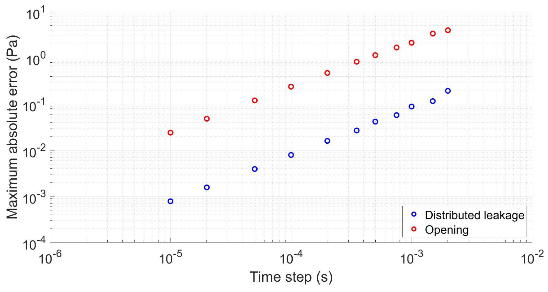
An analysis of the optimum time step considering computation speed and solution accuracy was performed. The solution to the MDE equations for one particular case, run and house, and case, run, house and opening was found using the Dormand–Prince adaptive Runge–Kutta method for the distributed leakage and opening cases, respectively. The MATLAB^® function ode45, which implements the Dormand–Prince method, was used for the calculation with absolute and relative tolerances ${10}^{-6}$ and ${10}^{-3}$, respectively.

This solution was assumed to be a good approximation of the exact solution. Then, the maximum error of the solutions of the faster iterative backward difference method was calculated by comparing to this “exact solution” for different time steps. Figure 9 shows the maximum absolute error in the internal pressure as a function of the time step for the distributed leakage and the opening case. Time steps $Dt={10}^{-3}\mathrm{s}$ and $Dt={10}^{-4}\mathrm{s}$ for distributed leakage and opening scenarios were selected to keep the error lower than the uncertainty of the pressure measurements, that is, $\pm 0.3$ Pa.

Simulations for each case, run, and house for the distributed leakage scenario and case, run, house, and opening for the single opening scenario were performed. In total, 7560 opening simulations and 672 distributed leakage simulations were completed.

4. Results

In this section, the maximum nominal ratios of the components of the overall forces on the whole houses $r_{F,nom,max}$ and net pressures on the surface of the houses $r_{p,nom,max}$ are reported for different comparison scenarios. Recall that the nominal force and pressure ratios have been defined in Equation (14) and Equation (15), respectively. The lateral forces $F_x$ and $F_y$ are the forces along the ridge of the house and transversal to the ridge, respectively, while $F_z$ is the vertical or uplift force (see Figure 6). For pressures, only the net pressure acting in the outwards direction is considered. The net pressure is calculated as the difference between external and internal pressure.

ASCE/SEI 7–22 proposes three enclosure classifications relevant to this research, i.e., sealed, enclosed, and partially enclosed. Each classification leads to a different internal pressure value assignment, as explained in Section 3. Since the internal pressure coefficient in the enclosed and partially enclosed classifications is the same, only the partially enclosed condition is analyzed.

The comparison offered here is performed between force components and net pressures calculated using ASCE/SEI 7–22 in the sealed and partially enclosed conditions on the one hand, and on the other hand, the ones calculated from physical simulations in the WindEEE Dome under the three different simulated internal pressure scenarios described in Section 3.4. The simulated internal pressure scenarios are “Sealed”, “Distributed Leakage”, and “Opening”. There is a clear equivalence between the sealed scenario and the sealed classification in ASCE/SEI 7–22. The ASCE/SEI 7–22 partially enclosed classification has its counterpart in the opening scenario, while the distributed leakage scenario may be associated with the enclosed classification. Two examples of the calculations of $r_{F,nom,max}$ and $r_{p,nom,max}$ are given next.

Suppose we want to compare the maximum uplift force ($F_z$) induced by the EF3-rated tornado, as calculated from physical simulation data in a scenario with one dominant opening, with the uplift design force calculated using ASCE/SEI 7–22 for the partially enclosed classification. The diagram in Figure 10 illustrates the process for calculating $r_{Fz,nom,max}$ in this example. We first select the cases simulating the translating EF3 equivalent tornado, that is, W3E1, W3E2, W3E11, W3E12, W3E16, and W3E17. The uplift force time histories on the roofs of each of the eight houses are calculated for each opening location across all runs. The peak forces in each run for all unique combinations of case, house, and opening are identified, as shown by the black triangles in the uplift force time history plots in Figure 10. These peaks are then fitted to a type-I GEVD using Lieblein’s BLUE method. The nominal extremes are calculated as the 78th percentile of the distribution and converted to full scale using dimensional analysis. Concurrently, the uplift design force for the entire roof of each house is estimated using the ASCE/SEI 7–22 standard for the partially enclosed classification. Finally, the ratios of the simulated to design forces are computed, and the maximum ratio is determined.

The process for calculating the maximum pressure ratios is similar. Suppose we want to compare the net pressure induced in zone 3 by the EF2 equivalent tornado in the sealed scenario against the design pressure calculated in the sealed classification using ASCE/SEI 7–22. We first select the cases simulating the translating EF2 equivalent tornado: W3E3, W3E4, W3E9, and W3E10. For each run in each case, the pressure time histories for all taps in zone 3 on all houses are computed. For the sealed scenario, the internal pressure in all cases is fixed. The peaks are found and grouped by unique combinations of case and tap. For instance, the peaks of the net pressure time histories at tap 320—located in zone 3 on the roof of House 1—for the 5 runs in case W3E3 are found. This set is then fitted to a type-I GEVD, and the nominal value is calculated as the 78th percentile of the distribution in full scale. In parallel, the design pressures in zone 3 are estimated following ASCE/SEI 7–22 for the sealed classification. The nominal ratios are computed, and the maximum ratio is determined.

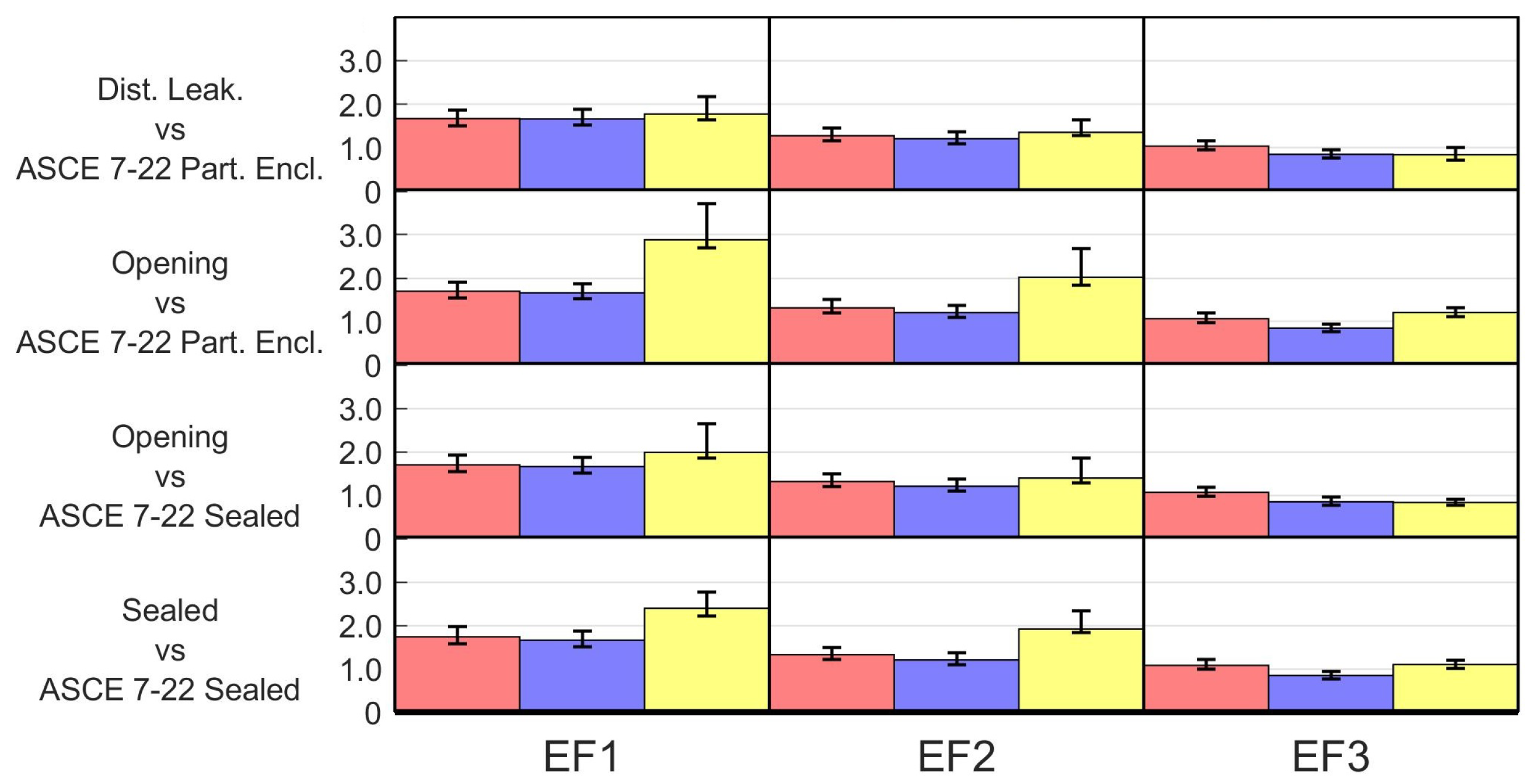
4.1. MWFRS

Figure 11 shows the ratios of the force components on the whole house. Here, “DistLeak”, “Opening” and “Sealed” denote “Distributed leakage”, “Opening” and “Sealed” internal pressure scenarios, while “PartEnc” and “Sealed” denote partially enclosed and sealed enclosure classification. The same information is presented in table form in Appendix A, in

Table A1. Ratios of the overall force components calculated from physical simulation measurements to the calculations performed according to ASCE/SEI 7–22. In parentheses are the 90% confidence intervals and in bold are the ratios that are higher than 1.0.

		EF1			EF2			EF3
	Fx	Fy	Fz	Fx	Fy	Fz	Fx	Fy	Fz
DistLeak vs ASCE/SEI 7–22_PartEnc	1.67 (1.47,1.83)	1.66 (1.44,1.80)	1.77 (1.37,1.91)	1.27 (1.09,1.39)	1.20 (1.05,1.31)	1.35 (1.06,1.42)	1.04 (0.91,1.13)	0.85 (0.75,0.93)	0.84 (0.68,0.96)
Opening vs ASCE/SEI 7–22_PartEnc	1.70 (1.50,1.85)	1.66 (1.44,1.79)	2.88 (2.04,3.07)	1.31 (1.12,1.42)	1.20 (1.04,1.31)	2.02 (1.36,2.19)	1.06 (0.93,1.15)	0.85 (0.75,0.93)	1.21 (1.10,1.30)
Opening vs ASCE/SEI 7–22_Sealed	1.70 (1.48,1.85)	1.66 (1.44,1.81)	1.98 (1.32,2.12)	1.31 (1.13,1.42)	1.20 (1.04,1.31)	1.39 (0.93,1.51)	1.06 (0.94,1.16)	0.85 (0.75,0.93)	0.83 (0.75,0.89)
Sealed vs ASCE/SEI 7–22_Sealed	1.74 (1.51,1.90)	1.66 (1.45,1.80)	2.39 (2.01,2.58)	1.33 (1.16,1.44)	1.20 (1.04,1.32)	1.92 (1.51,2.01)	1.08 (0.94,1.17)	0.85 (0.75,0.93)	1.10 (1.00,1.18)

.

The ratios of lateral forces calculated for the EF1-rated tornado are approximately 1.7, for the EF2-rated tornado approximately 1.3, and for the EF3-rated tornado around 1.0. The values of lateral force ratios are close together for the same EF rating and component, regardless of the internal pressure scenario, which can be explained by the fact that the internal pressure value does not influence the value of overall lateral forces. In most comparisons, the ratios for $F_x$ are higher than the ratios for $F_y$, but similar.

The values of the uplift force ratios are all higher than 1.0, except for the EF3-rated tornado. For each EF rating, the ratios for uplift force are the lowest in the comparison between the distributed leakage scenario and the ASCE/SEI 7–22 partially enclosed classification. Slightly higher values are found in the comparison between the opening scenario and ASCE/SEI 7–22 sealed classification. The highest values are found when comparing the opening scenario and the ASCE/SEI 7–22 partially enclosed classification, followed closely by the comparison between the sealed scenario and ASCE/SEI 7–22 sealed classification. This indicates that the use of an internal pressure ${C_p}_i=+0.55$ is insufficient to account for the effect of openings, and that the value ${C_p}_i=+1.0$ is also insufficient to account for the effect of the APD in sealed scenarios.

In the event of a breach in the envelope, the uplift force can change dramatically, reaching values of ratios as high as 2.88 for the EF1-rated tornado in the comparison between the opening scenario and ASCE/SEI 7–22 partially enclosed classification. These values decrease as the rating increases: 2.02 for the EF2-rated tornado and 1.21 for the EF3-rated tornado. This represent an increase between 44% and 63% in the uplift force from the distributed leakage scenario to the opening scenario, which highlights the importance of keeping the integrity of the building’s envelope.

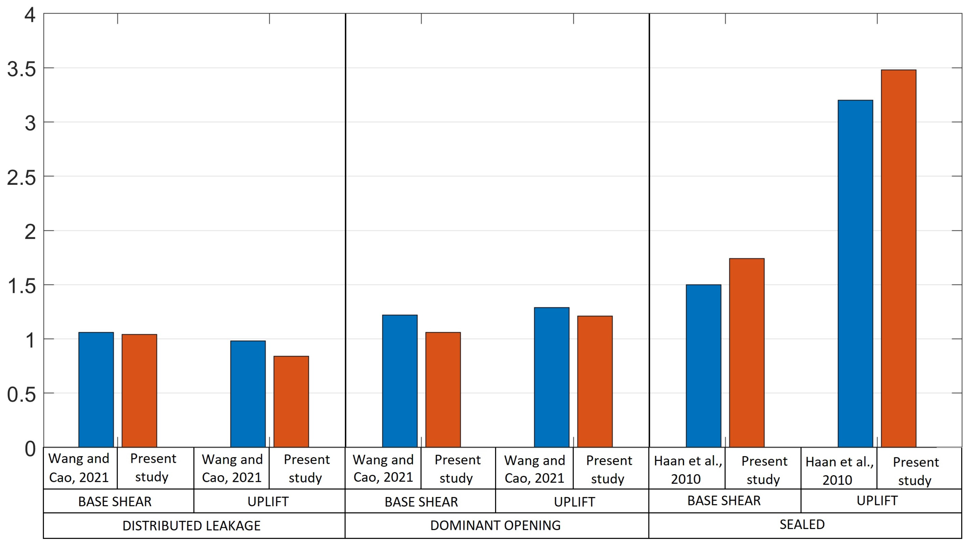
Comparison with Previous Studies

Figure 12 presents the comparison of the maximum ratios of the base shear and uplift forces on the whole houses between measurements and code-based calculation reported by Wang and Cao [29] and Haan Jr et al. [19], and this research. In order to make a fair comparison, the analogous ratios to the ones calculated by the cited authors among the ratios calculated in this research are identified.

Wang and Cao [29] compared the tornado-induced loads on a low-rise building obtained from wind tunnel simulations with the guidelines from ASCE/SEI 7–16. They measured the internal pressure and simulated four cases, which represent two internal pressure scenarios, i.e., distributed leakage and one dominant opening. The swirl ratio used in their research was 0.72, which corresponds to an EF3-rated tornado according to the authors. Accordingly, their results are compared in two ways. First, their distributed leakage vs. ASCE/SEI 7–16 is compared to the Dist.Leak. vs. ASCE/SEI 7–22 Partially Enclosed for the EF3 tornado in this research and their one dominant opening vs. ASCE/SEI 7–16 was compared to the Opening vs. ASCE/SEI 7–22 Partially Enclosed for the EF3-rated tornado in this research.

Haan Jr et al. [19] calculated the ratios between the overall forces on a simple gable roof low-rise building and the provisions in ASCE/SEI 7–05. It is important to note that ASCE/SEI 7–05 did not have provisions nor guidelines for tornado-resistant design; therefore, the authors adapted the parameters, originally intended for ABL flows, to fit tornadoes. In addition, they simulated several swirl ratios and reported the maximum base shear and uplift ratios. They found that the maximum ratio decreased as the swirl ratio increased; therefore, the maximum ratio was found at the lowest swirl ratio. Also, they did not consider internal pressure; consequently, their results are equivalent to the sealed scenario in this research. Therefore, their ratio for the lowest swirl ratio is compared to the Sealed vs. ASCE/SEI 7–22 Partially Enclosed for the equivalent EF1 in this study.

Overall, the comparison shows strong agreement between studies. This study reports lower values of the ratios than Wang and Cao [29] in the distributed leakage and dominant opening in both the base shear and the uplift force. In the sealed scenario, the agreement between the maximum ratios for base shear and uplift force is also very good, with slightly higher values for this study.

4.2. Components and Cladding (C & C)

Here, in Figure 13 and

Table A2. Ratios of the pressures in C&C zones calculated from physical simulation measurements to the calculations performed according to ASCE 7–22. In parentheses are the 90% confidence intervals and in bold are the ratios that are higher than 1.0.

				Zones
	Rating	1	2	3	4	5
Dist. Leak.	EF1	1.42 (0.99,1.60)	1.65 (1.10,1.77)	0.61 (0.49,0.67)	1.37 (0.96,1.52)	1.77 (1.04,2.13)
vs	EF2	0.92 (0.80,0.98)	1.24 (1.06,1.39)	0.55 (0.44,0.63)	1.54 (1.18,1.82)	1.33 (1.01,1.56)
ASCE/SEI 7–22 Part.Encl. & Encl.	EF3	0.77 (0.58,0.88)	1.03 (0.82,1.15)	0.44 (0.40,0.48)	0.86 (0.63,1.05)	1.11 (0.99,1.19)
Dist. Leak.	EF1	1.15 (0.80,1.29)	1.43 (0.96,1.54)	0.55 (0.44,0.61)	1.03 (0.73,1.15)	1.38 (0.81,1.66)
vs	EF2	0.74 (0.65,0.79)	1.08 (0.92,1.21)	0.50 (0.40,0.57)	1.16 (0.89,1.37)	1.04 (0.79,1.22)
ASCE/SEI 7–22 Sealed	EF3	0.62 (0.47,0.71)	0.89 (0.71,1.00)	0.40 (0.36,0.43)	0.65 (0.48,0.79)	0.87 (0.78,0.93)
Sealed	EF1	2.07 (1.57,2.27)	2.03 (1.53,2.18)	1.05 (0.81,1.26)	2.38 (1.83,2.57)	2.48 (1.78,2.86)
vs	EF2	1.53 (1.22,1.66)	1.59 (1.40,1.67)	1.00 (0.85,1.07)	2.28 (1.87,2.63)	1.96 (1.61,2.26)
ASCE/SEI 7–22 Part.Encl. & Encl.	EF3	1.15 (0.96,1.24)	1.35 (1.11,1.50)	0.75 (0.69,0.81)	1.48 (1.21,1.68)	1.65 (1.50,1.74)
Sealed	EF1	1.68 (1.27,1.83)	1.76 (1.33,1.90)	0.93 (0.72,1.11)	1.80 (1.38,1.93)	1.93 (1.39,2.24)
vs	EF2	1.23 (0.99,1.34)	1.38 (1.21,1.45)	0.88 (0.75,0.95)	1.72 (1.41,1.98)	1.53 (1.26,1.77)
ASCE/SEI 7–22 Sealed	EF3	0.93 (0.78,1.01)	1.17 (0.96,1.30)	0.66 (0.61,0.72)	1.11 (0.91,1.27)	1.28 (1.17,1.36)
Opening	EF1	1.77 (1.12,1.93)	1.83 (1.27,1.95)	0.93 (0.76,1.00)	2.02 (0.87,2.67)	1.99 (1.14,2.46)
vs	EF2	1.25 (0.89,1.36)	1.35 (1.18,1.42)	0.84 (0.68,0.96)	1.97 (1.60,2.23)	1.69 (1.37,1.92)
ASCE/SEI 7–22 Part.Encl. & Encl.	EF3	0.92 (0.76,0.99)	1.15 (0.91,1.31)	0.68 (0.62,0.74)	1.34 (1.10,1.40)	1.44 (1.29,1.53)
Opening	EF1	1.43 (0.91,1.56)	1.59 (1.11,1.70)	0.83 (0.67,0.89)	1.52 (0.65,2.01)	1.55 (0.89,1.92)
vs	EF2	1.01 (0.72,1.10)	1.18 (1.02,1.23)	0.74 (0.60,0.85)	1.48 (1.21,1.68)	1.32 (1.07,1.50)
ASCE/SEI 7–22 Sealed	EF3	0.74 (0.62,0.80)	1.00 (0.79,1.14)	0.60 (0.55,0.66)	1.01 (0.83,1.06)	1.12 (1.01,1.19)

in Appendix A, the ratios of pressure in different zones and EF equivalent rating are presented. Observe that the colors in Figure 13 represent the equivalent rating of the tornado, in contrast to Figure 11, where the colors represent the different components of the overall forces. The zones are defined in Chapter 30 of ASCE/SEI 7–22, Figures 30.3-1, and 30.3-2C, and can be seen in Figure 4. The maximum absolute values of the pressure coefficients are utilized. These values correspond to the least EWA, i.e., less than $0.9{\mathrm{m}}^2$ for all zones. Hence, the values of the external pressure coefficient $G{C}_p$ are the following: −1.5 for zone 1, −2.5 for zone 2, −3.0 for zone 3, −1.1 for zone 4 and −1.4 for zone 5.

The two most relevant C&C comparisons reported in this article are between the Distributed Leakage scenario and the ASCE/SEI 7–22 Partially Enclosed and Enclosed classification and between the Opening scenario and ASCE/SEI 7–22 Partially Enclosed and Enclosed classification. These comparisons are significant because “Distributed Leakage” and “Opening” represent the two most common internal pressure scenarios during tornado impacts, with the enclosed or partially enclosed classifications being the most typical for the majority of residential buildings.

In the comparison between the Distributed Leakage scenario and the ASCE/SEI 7–22 Partially Enclosed and Enclosed classification, the ratio in Zone 1 is higher than 1.0 for EF1-rated tornadoes, while the ratios in the remaining zones are lower. In Zone 2, the ratios for EF1- and EF2-rated tornadoes exceed 1.0, whereas in Zone 3, they are below 1.0. On the walls, most ratios exceed 1.0, except for Zone 4 with EF3-rated tornadoes. Although using a $G{C}_p=-3.0$ in Zone 3 results in safe provisions, it is evident that in all other zones, the load provisions are lower than those obtained through physical simulations. This observation may lead to a revision of the pressure coefficients used for tornadoes or improve the corrections used.

For the comparison between the Opening scenario and ASCE/SEI 7–22 Partially Enclosed and Enclosed classification, in Zones 1 and 2, the ratios are higher than 1.0 for all EF-ratings except for the ratio for EF3-rated tornadoes in Zone 1. Again, the ratios in Zone 3 are all lower than 1.0, while all ratios on the walls, that is, Zones 4 and 5, exceed 1.0. When transitioning from the comparison between the Distributed Leakage scenario and the ASCE/SEI 7–22 Partially Enclosed and Enclosed classification to the comparison with the Opening scenario, there is a generalized increase in the ratios. In Zone 1, the increase ranges from 20% to 36%; in Zone 2, the increase is more modest, between 9% and 12%. In Zone 3, the ratios increase by approximately 50%, although they remain below 1.0. Zone 4 experiences an increase in loads ranging from 28% to 56%, while Zone 5 shows growth between 12% and 30%. This result underscores the need to keep the integrity of the envelope to reduce the overall loads on C&C.

Almost all ratios on wall zones 4 and 5 are higher than 1.0. A maximum ratio of 2.48 is registered in the comparison between the Sealed scenario and the ASCE/SEI 7–22 Partially Enclosed and Enclosed classification, for the EF1-rated tornado in zone 5. In the comparison between the Opening scenario and ASCE/SEI 7–22 Partially Enclosed and Enclosed classification, the ratios are between 1.99 and 2.02 for the EF1-rated tornadoes, between 1.69 and 1.97 for the EF2-rated tornadoes, and between 1.34 and 1.44 for the EF3-rated tornadoes. This is consistent with the observation of sidewalls blowing outwards during tornado events when openings are present [52].

The comparison between the Sealed scenario and the ASCE/SEI 7-22 Sealed classification yields similar values to the comparison between the Opening scenario and the ASCE/SEI 7-22 Partially Enclosed and Enclosed classifications. However, an overall reduction in the values is observed.

The difference between the comparison of the Opening scenario with the ASCE/SEI 7–22 Partially Enclosed and Enclosed classification and its comparison with the ASCE/SEI 7–22 Sealed classification lies solely in the internal pressure coefficient used: ${C_p}_i=+0.55$ in the first case and ${C_p}_i=+1.0$ in the second. The higher internal pressure coefficient results in a reduction in the ratios by 24% in Zone 1, 15% in Zone 2, 13% in Zone 3, 33% in Zone 4, and 28% in Zone 5. Notably, the ratios on wall zones are the ones reduced the most, suggesting that a combination of revised values of ${C_p}_i$ and $G{C}_p$, or correction factors could be employed to enhance the standard’s performance in providing safe tornado-induced load provisions.

4.3. Ratio Uncertainty Estimation

The most important sources of uncertainty in the reported ratios are (1) the small sample size due to the number of runs available for each case, i.e., between five and nine runs, (2) the value of the velocity gust factor, (3) measurement uncertainties, and (4) the statistical model adopted to describe the distribution of the maximums, i.e., type-I GEVD.

The limited sample size arises from the cost and time constraints imposed by this type of physical simulation at the WindEEE Dome. The number of samples necessary to eliminate the small sample size effect is unknown; however, Chen et al. [53] concluded that the statistical estimates based on 200 repetitions were accurate. This value is extremely high and exceedingly expensive to achieve in a study like this. For comparison, Haan Jr et al. [19] and Case et al. [21] used ten runs and Roueche et al. [26] used five runs.

The determination of the minimum sample size for GEVD quantile estimation was studied by Cai and Hames [54]. They developed a method that uses the Shapiro–Wilk normality test on the bootstrapped maximum likelihood estimators (MLEs) of the distribution parameters for a prescribed significance level $\alpha$. The number of samples must be increased until the p-value > $\alpha$, which would indicate that the null hypothesis (normality) cannot be rejected. With this criterion, for $\alpha =0.05$, both five and nine runs are insufficient to adequately describe the population of peaks.

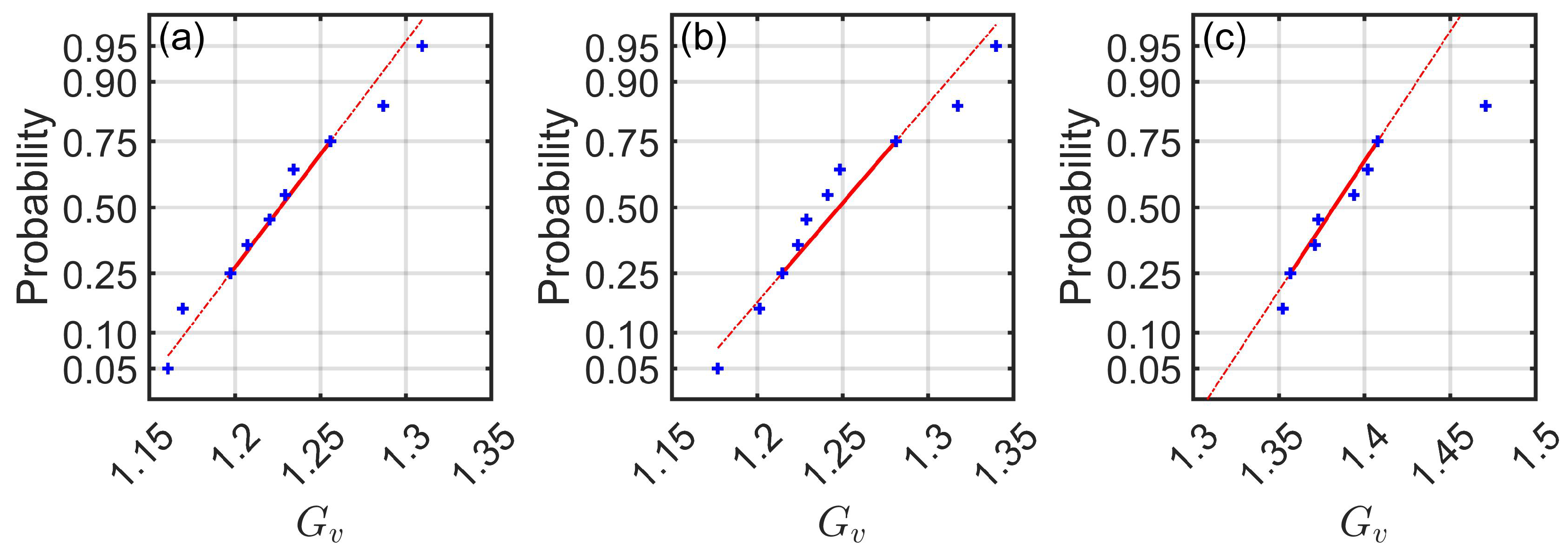
As was mentioned before, the value of the tornado velocity gust factor adopted can have a significant influence on the ratios. Since the gust factors are calculated as the average of the ratios between peak and mean in segments of the velocity time history measured in stationary TLVs, if the underlying distribution is normal, the gust factor must have a Student-t distribution with $n-1=10-1=9$ degrees of freedom, and $\sigma =S/\sqrt{n}$ and $\mu =\overline{x}$, where $S^2$ and $\overline{x}$ are the sample variance and mean, respectively. The assumption that the underlying distribution is normal is reasonable, as can be observed from the normal probability plots in Figure 14. 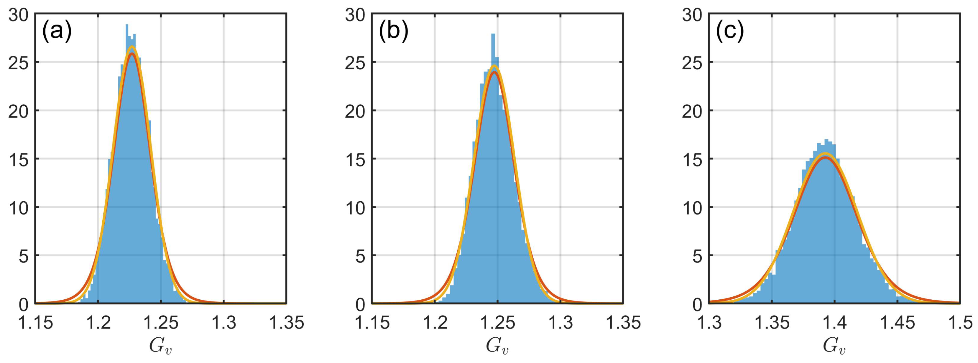Figure 15 shows normalized histograms of the bootstrapped velocity gust factors along with the Student-t and normal distribution with $\sigma$ and $\mu$ calculated, as explained before, showing good agreement.

Measurement uncertainties are judged to be of a lower order than the uncertainties generated by the low number of runs and the velocity gust factor and therefore are not evaluated.

It is assumed that the maximums have type-I GEVD. The epistemic uncertainty associated with this assumption can be reduced if additional samples are available, which is beyond the scope of this research.

The uncertainty in the ratios is estimated using the parametric bootstrap method [55]. The steps of the procedure are as follows:

• From the list of maxima, i.e., the maxima on each repetition (run), a high number (10,000) of resamples (with replacement) are found.
• For each resample, a set of parameters of the type-I GEVD are obtained by fitting them using Lieblein’s BLUE method.
• With each set of parameters, the nominal peak (78th percentile) is obtained.
• From a Student-t distribution with $\sigma$ and $\mu$ calculated as explained before, values of the velocity gust factor are randomly generated (10,000).
• A set of 10,000 ratios is calculated using the nominal peaks and velocity gust factors.
• The two-sided 90% confidence interval is found from the 5th and 95th percentiles. These limits are used to report uncertainties in the ratios in Figure 11 and Figure 13, Table A1 and Table A2.

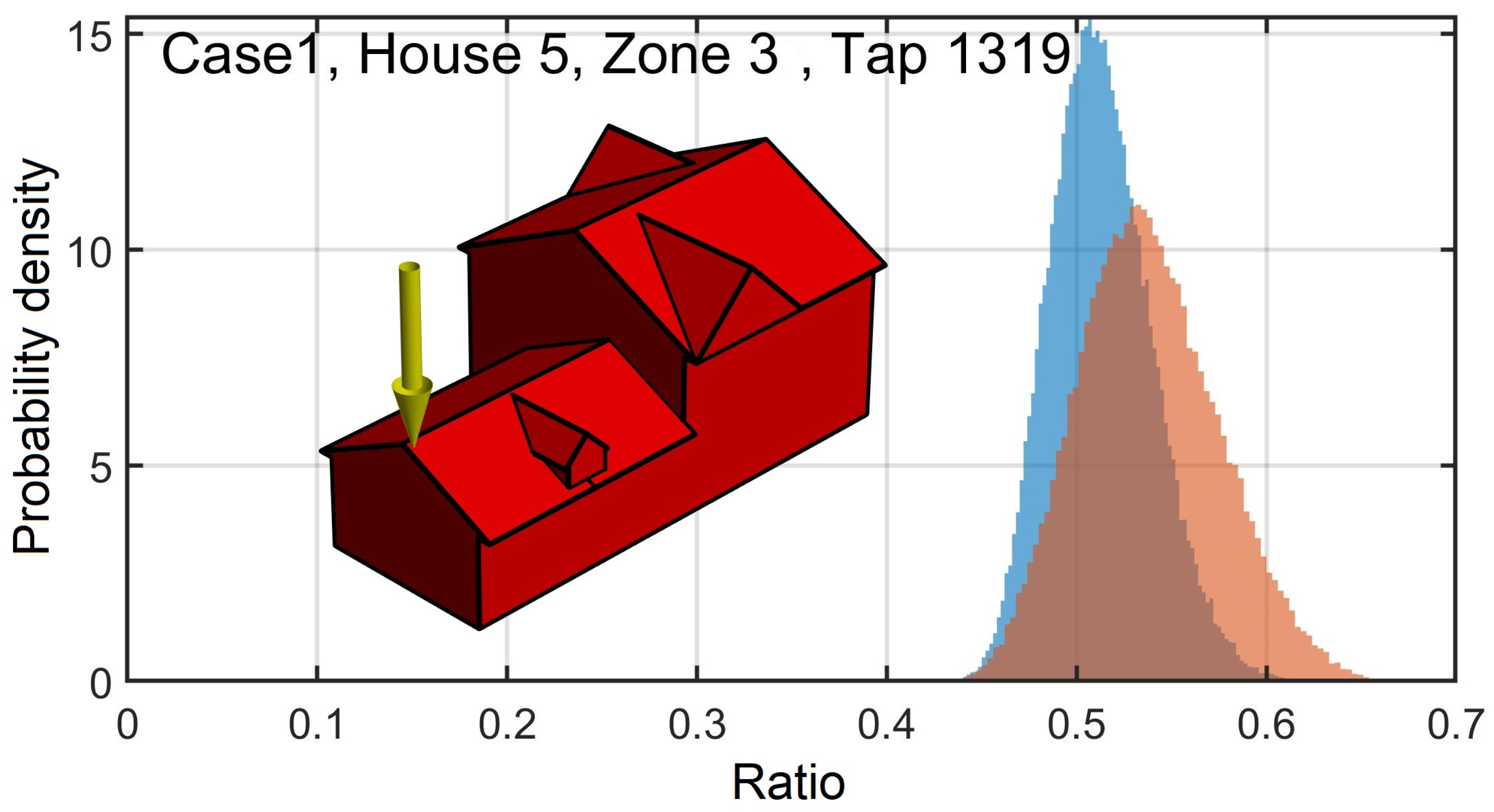
Figure 16 shows the normalized histograms of the 78th percentile of the ratio of pressure at Tap 1319, Zone 3, House 5, and Case W3E1, calculated from physical simulation to those calculated using ASCE/SEI 7–22 Partially Enclosed classification using nine runs (blue) and five runs (orange). This highlights the reduction in the uncertainty in the ratios by increasing the number of runs.

Finally, it is important to note that the code calculations are based on an open terrain exposure, whereas the simulated TLVs develop over a smooth, flat surface. This mismatch may introduce additional uncertainty into the results. The effect of surface roughness on the vertical tangential velocity profile is complex; in most cases, roughness shifts and amplifies the peak of the profile [56]. This complexity makes it difficult to draw confident conclusions about the behavior of the ratios under varying roughness conditions.

5. Conclusions

The goal of this study was to compare the design tornado-induced loads provided by ASCE/SEI 7–22 against what would be experienced by real-world shaped low-rise residential buildings forming a community during tornado events of different intensities.

Physical simulation in the WindEEE Dome at the UWO was employed to investigate this issue. Pressures on the surface of eight model houses in a community were measured while interacting with several translating TLVs with different characteristics, representative of EF1-, EF2- and EF3-rated tornadoes, with a diversity of paths and trajectories. Three internal pressure scenarios were simulated numerically using the MDE model. Net pressures on the surface of the houses and the overall forces on the whole houses were calculated.

The tornado velocity gust factor was identified as a crucial parameter for translating loads from the model scale to full scale. To calculate this factor, a method based on stationary TLV velocity measurements at the RMW was developed. The calculated tornado velocity gust factor values decrease as the equivalent EF-rating of the studied tornado increases. This trend is likely due to the intensified wandering effect at lower swirl ratios observed in the TLVs simulated in the WindEEE Dome. While tornado wandering may naturally occur, it has not been characterized, raising questions about whether the wandering motion of TLVs in the WindEEE Dome accurately represents the random movement of real tornadoes. However, it is important to note that the decrease in all ratios with increasing EF-rating is not due to the reduction in the tornado velocity gust factor as the swirl ratio increases. High tornado velocity gust factors result in low ratios, and vice versa. Therefore, the higher ratios at low swirl ratios, despite the high gust factors, suggest that amplified loads at low swirl ratios relative to the mean maximum tangential velocity squared are responsible for this effect. Given the uncertainties inherent in the calculation of tornado velocity gust factors, a method is provided to translate the results of this study to alternative gust factors.

The ratios of lateral force are approximately 1.7, 1.3, and 1.0 for the EF1-, EF2-, and EF3-rated tornadoes, respectively, regardless of the comparison analyzed. This effect was expected, since the internal pressure does not affect the overall lateral forces. The lowest ratios for uplift force are found in the comparison between the Distributed leakage scenario and the ASCE/SEI 7–22 Partially Enclosed classification; however, except for the EF3-rated tornado, the ratios are all higher than 1.0. This suggests that when the building envelope remains intact, the MWFRS design provisions for structures classified as Enclosed or Partially Enclosed demonstrate the best performance. The worst performance of the ASCE/SEI 7–22 provisions for Enclosed or Partially Enclosed buildings occurs in the Opening scenario. In the event of a breach in the envelope, the uplift force can increase by 44% to 63%, emphasizing the critical importance of maintaining the integrity of the building envelope to minimize uplift forces on the roof. Additionally, when an opening is present, the design internal pressure coefficient used in the Enclosed and Partially Enclosed classifications is insufficient to account for the higher internal pressure induced by the flow through the opening. For buildings classified as Sealed, the uplift force ratios in the Sealed scenario are 2.39, 1.92, and 1.10 for EF1-, EF2-, and EF3-rated tornadoes, respectively, which indicates that the internal pressure coefficient used in the Sealed classification may be insufficient to account for the APD.

The comparison of pressures between the Distributed Leakage scenario and the ASCE/SEI 7–22 Partially Enclosed and Enclosed classification shows that although using a $G{C}_p=-3.0$ in Zone 3 results in safe provisions, it is evident that in all other zones, the load provisions are lower than those obtained through physical simulations. This observation may lead to a revision of the pressure coefficients used for tornadoes or improve the corrections used. When transitioning from the previous comparison to the comparison with the Opening scenario, there is a generalized increase in the ratios that ranges from 12% to 56%. This is in line with the conclusion obtained from the observed increase in the overall uplift force ratios in the same situation, underscoring the need to keep the integrity of the envelope to reduce the overall loads on C&C. Minimizing the occurrence of breaches in the envelope is critical to reduce loads, and to avoid water penetration. Almost all pressure ratios on wall zones 4 and 5 are higher than 1.0; in particular, when an opening is present, the ratios are between 1.34 and 2.02. This is consistent with the observation of sidewalls blowing outwards during tornado events when openings are present [52].

Using an internal pressure coefficient of +1.0 in the Sealed classification, instead of the +0.55 value used in the Enclosed and Partially Enclosed classification, reduces the ratios by 24% in Zone 1, 15% in Zone 2, 13% in Zone 3, 33% in Zone 4, and 28% in Zone 5. Notably, the reductions are most significant in the wall zones, suggesting that revising the values of ${G{C}_p}_i$ and $G{C}_p$, or incorporating correction factors, could improve the standard’s ability to provide safer tornado-induced load provisions for C&C.

While we believe that testing the performance of the standard for real-world building geometries in a community provides valuable insights, testing isolated simplified gable roof buildings, such as the archetypes outlined in the standard, is also important and complementary to this study. Independent tests under different scenarios are needed to inform future editions of the standard’s tornado-induced load provisions.