Towards Bayesian Evaluation of Seroprevalence Studies ^†

Abstract

Bayes’ Theorem represents a mathematical formalization of the common sense. What we know about the world today is what we knew yesterday plus what the data told us. The lack of understanding of this concept is the source of many errors and wrong judgements in the current COVID-19 pandemic. In this contribution, we show how to use the framework of Bayesian inference to produce a reasonable estimate of seroprevalence from studies that use a single binary test. Bayes’ Theorem sometimes produces results that seem counter-intuitive at first sight. It is important to realize that the reality may be different from its image represented by test results. The extent to which these two worlds differ depends on the performance of the test (i.e., its sensitivity and specificity), and the prevalence of the tested condition.

1. Introduction

In the age of the coronavirus, various testing has become enormously widespread. Unfortunately, what has not become widespread is the understanding of the test results. The most common PCR test is used for the detection of the virus (more precisely its particular fragments) in a sample collected by a nasopharyngeal swab. The number of PCR positive cases can be used to assess the Case Fatality Rate (CFR) of the infection. CFR is the proportion of COVID-19 deaths in the diagnosed (i.e., PCR positive) population. However, CFR depends heavily on the testing strategy–any infection may reach the CFR of $100\%$ if only the deceased are tested. Thus, it is more sensible to estimate the Infection Fatality Rate (IFR) which is the proportion of COVID-19 deaths in the infected population, regardless whether the infection was detected or not. The IFR is always lower than CFR and it does not depend on the testing strategy. However, apart from the virus itself, IFR also depends on the characteristics of the population, state of health care, etc. To estimate the IFR, one must infer what proportion of the population has already met the virus.

One option to find the proportion of so far infected people is to test for the presence of antibodies against the coronavirus in a representative sample of the population. Many seroprevalence studies have been performed and their results helped to estimate the IFR of COVID-19, e.g., [1,2,3]. The meta-study by Ioannides [4] combined 61 larger sero-prevalence studies and reported the median IFR of $0.23\%$. In people under 70 years, the median IFR reached $0.05\%$. Both the numbers are likely to be overestimated because an unknown proportion of population defeats the virus on the level of cellular immunity (and probably even become immune) without producing antibodies at all [5]. This seems to be the case especially for children [6].

Despite the fundamental importance of various forms of testing, not enough attention has been paid to the correct interpretation of the test results. In this paper, we want to explain this issue in three successive steps of an increasing level of complexity. We use the example of antibody tests here, but the same logic should be used for any test, the results of which are converted to a binary answer (positive–negative). This applies to all antibody tests (laboratory or rapid tests), all PCR tests (full RT-qPCR, antigen testing, etc.), and many more coronavirus unrelated medical tests, or even health unrelated tests (such as AB testing [7]).

2. Antibody Primer

Some explanation of the mechanism of antibodies testing is needed. We use the example of the standard Enzyme-Linked Immunosorbent Assay (ELISA). This is a semiquantitative method which measures the amount of SARS-CoV-2 antibodies in a sample by detecting a color change of the sample resulting from a reaction. The color change is quantified by the optical density of the sample. The optical density is then divided by the optical density of a calibration sample (provided in each kit by the manufacturer) which contains a borderline concentration of the antibodies. The sample is considered positive, if the resulting Optical Density Ratio (OD Ratio) exceeds a threshold set by the manufacturer ($1.1$ in the case of Euroimmun ELISA kits) and negative, if the OD Ratio falls below a threshold ($0.8$ in the case of Euroimmun ELISA kits). OD Ratio values between the two thresholds are deemed inconclusive. ELISA assays are usually performed in batches of 96-well plates. Each plate contains one or two calibration samples and a few positive and negative controls.

There are several types of antibodies, each with a specific role in fighting the disease and thus each with specific dynamics. The most commonly measured antibodies are immunoglobulins A (IgA) and immunoglobulins G (IgG). The production of IgA antibodies starts 1–2 weeks from the infection and they last for at least several weeks. IgG are produced somewhat later but usually last for several months after the infection. There is considerable debate about the protective role of the antibodies and the possibility of a reinfection [8,9,10]. It is probable that some (possibly most) of reported reinfections are due to the false positivity or false negativity of one of the PCR tests. This provides further motivation for thinking clearly about the test results.

3. A Binary Test Primer

Each test with a binary outcome has a certain accuracy which is never perfect. Let us fix ideas by considering a single test with a binary outcome (positive or negative) for the presence of a specific antibody. In each tested subject, the antibody is either present ($A+$) or absent ($A-$), which we do not know. For each subject, the test may come out either positive ($T+$) or negative ($T-$), which is the observed result. The performance of the test may be significantly different for the $A+$ subjects and for the $A-$ subjects. Therefore, two numbers are needed to characterize the performance of any binary test. The sensitivity of the test is the accuracy on the $A+$ population, i.e., the probability that the test comes out positive provided the antibodies are, in fact, present. In terms of conditional probability, we can write $sens=p(T+|A+)$. On the other hand, the accuracy on the $A-$ population is called the specificity of the test. The specificity of the test is the probability that the test comes out negative provided the antibodies are absent. Thus, $spec=p(T-|A-)$. The prevalence of antibodies in the population is denoted by prev. It can be interpreted as the probability that the antibodies are present in a randomly chosen subject, i.e., $prev=p(A+).$

In practice, we test a subject and observe the test result, say $T+$. Since neither sens nor spec are perfect, a positive test result does not necessarily imply that the antibodies are presents (it may be a false positive). Thus, we want to make inference about the probability that the antibodies are present, provided the test came out positive. We use the Bayes’ Theorem to obtain

$$\begin{array}{ccc}\hfill p(A+|T+)& =& \frac{p(T+|A+\left)p\right(A+)}{p(T+|A+\left)p\right(A+)+p(T+|A-)p(A-)}=\hfill \\ & =& \frac{sens\times prev}{sens\times prev+(1-spec)\times (1-prev)}.\hfill \end{array}$$

It is important to realize that the posterior probability $p(A+|T+)$, i.e., the probability that a positively tested subject indeed has the antibodies, depends not only on the parameters of the test (sens and spec) but also on the prevalence. For example, the Euroimmun ELISA test for IgA anti-SARS-CoV-2 antibodies has a declared sensitivity of $98.6\%$ and specificity of $92.0\%$. If the prevalence is assumed to be around $1\%$ (as it was the case at the very beginning of the pandemic), a positive test result yields the posterior probability $p(A+|T+)$ of approximately $11\%$. Thus, about 9 out of 10 positive test results are false positives! If the prevalence rises to $10\%$ (a sensible figure after the first wave of the pandemic), the posterior $p(A+|T+)$ increases to about $58\%$. Once prevalence reaches $30\%$ (only the hardest hit regions may have reached this figure), the posterior grows further to $85\%$.

This example represents the step zero in understanding seroprevalence studies and suggests a careful way of interpreting binary test results is needed: A positive test does not necessarily imply that antibodies are present in the tested subject, it merely increases the probability that it is so. The posterior probability is given by the Bayes’ Theorem and it depends on the sensitivity and specificity of the test but also on the prevalence of the antibodies.

4. A Single Test Study

In a typical seroprevalence study, the question is how widespread a certain antibody is in a given population. Thus, we want to make inference on the prevalence. A test of known parameters is used and a random sample of N subjects is drawn from the population. The study yields data which consist of K positive test results and $N-K$ negative test results. The Bayes’ Theorem–this time written in terms of probability densities [11]–states that

$$p\left(prev\right|data)\propto p(data\left|prev\right)p\left(prev\right).$$

(1)

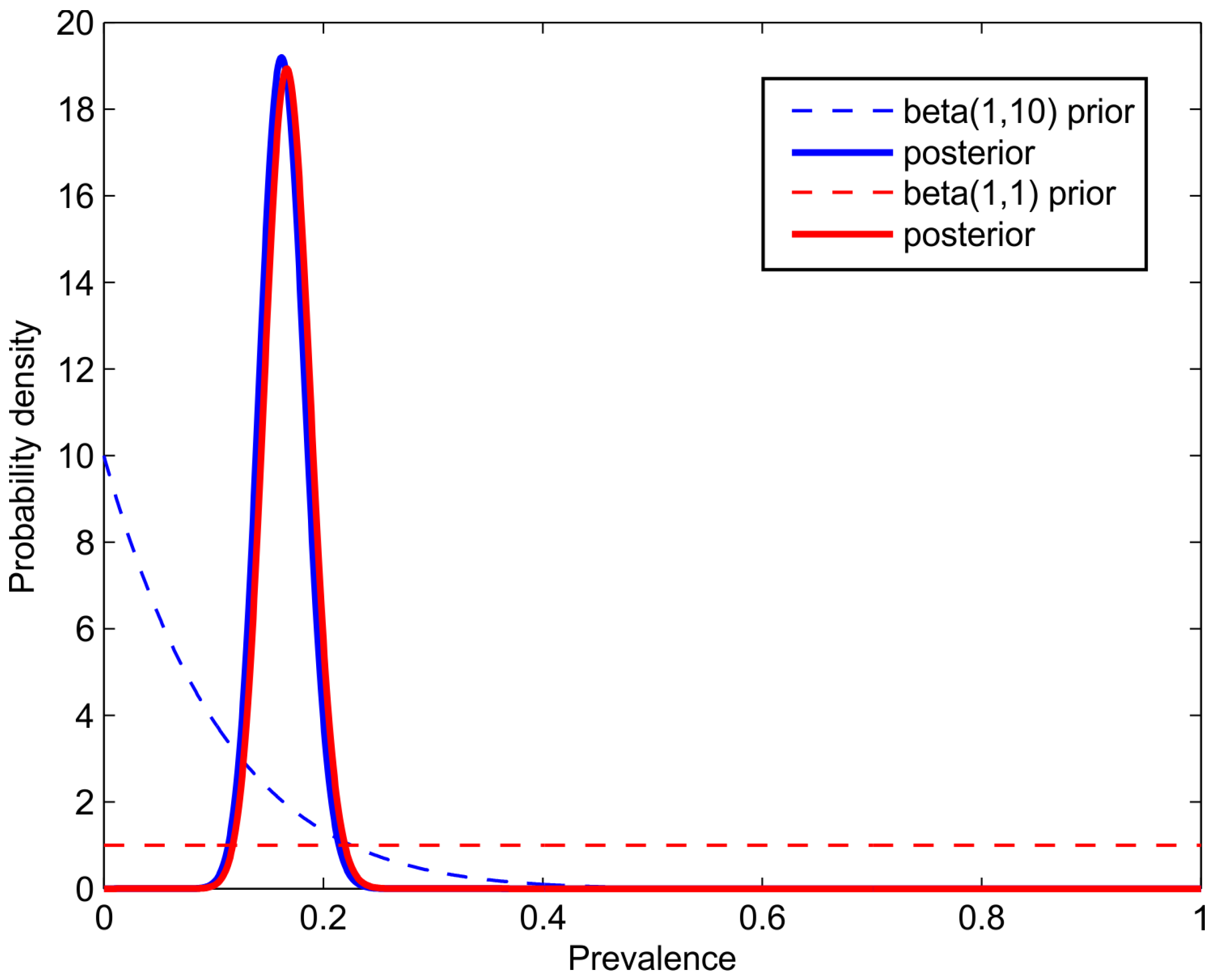
The proportional sign (∝) means that the posterior density $p\left(prev\right|data)$ must be normalized to a unit area. The posterior density represents a degree of belief about the prevalence, taking into account all the available data. Some assumption must be made about the prevalence that we want to estimate. This is the first principle of Bayesian inference–you cannot make inference without assumptions. It is sensible to model the prior density $p\left(prev\right)$ as a beta distribution centered around our prior beliefs. For example, if the study is performed at the very beginning of the pandemic, the prevalence is almost certainly very low, and so $p\left(prev\right)=beta(1,10)$ may be a sensible prior (see Figure 1).

Now let us evaluate the likelihood, i.e., $p\left(data\right|prev)$. The likelihood is interpreted as the probability of obtaining the observed data if the true prevalence was known and equal to prev. This is a rather simple calculation because

$$p\left(data\right|prev)\propto {\left[p(T+|prev)\right]}^K{\left[p(T-|prev)\right]}^{N-K}.$$

Both the terms are easy to evaluate:

$$\begin{array}{ccc}\hfill p(T+|prev)& =& p(T+|A+,prev\left)p\right(A+\left|prev\right)+p(T+|A-,prev\left)p\right(A-\left|prev\right)=\hfill \\ & =& p(T+|A+\left)p\right(A+\left|prev\right)+p(T+|A-\left)p\right(A-\left|prev\right)=\hfill \\ & =& sens\times prev+(1-spec)\times (1-prev).\hfill \end{array}$$

Analogously,

$$\begin{array}{ccc}\hfill p(T-|prev)& =& p(T-|A+,prev\left)p\right(A+\left|prev\right)+p(T-|A-,prev\left)p\right(A-\left|prev\right)=\hfill \\ & =& p(T-|A+\left)p\right(A+\left|prev\right)+p(T-|A-\left)p\right(A-\left|prev\right)=\hfill \\ & =& (1-sens)\times prev+spec\times (1-prev).\hfill \end{array}$$

Combining all the above, the likelihood becomes

$$\begin{array}{ll}p\left(data\right|prev)=& {[sens\times prev+(1-spec)\times (1-prev)]}^K\times \\ & {[(1-sens)\times prev+spec\times (1-prev)]}^{N-K}.\end{array}$$

This is an explicit expression that can directly be evaluated. In practice, the logarithm of the likelihood is evaluated to avoid the problem of multiplying small numbers. Figure 1 shows the results of an artificial example with $N=1000$ and $K=200$ for a test with the parameters $sens=0.7$ and $spec=0.9$.

Now consider the realistic setting of $sens=0.986$ and $spec=0.920$ for the anti-SARS-CoV-2 IgA ELISA assay. Let us assume that in a sample of $N=1000$ subjects, we obtained $K=100$ positive results. A careless estimate of the seroprevalence would yield $prev\sim K/N=10\%$. However, the correct computation (with the $beta(1,10)$ prior) reveals that the mean of the posterior is $2.2\%$–an almost five times lower number. The probability that the true prevalence exceeds $5\%$ is less than $0.01$, and the probability that the true prevalence exceeds $9\%$ is ${10}^{-8},$ i.e., the careless seroprevalence estimate $K/N$ is all but impossible! This is consistent with the observation of the previous section that in the environment of low prevalence, most of the positive test results are false positives. This shows that seroprevalence studies must be evaluated correctly because the careless estimate of the prevalence by the fraction of positive test results ($prev\sim K/N$) is usually completely meaningless.

5. Conclusions

We have shown how to use the framework of Bayesian inference to produce reasonable estimates of seroprevalence from studies that use a single binary test. Although the Bayes’ Theorem represents only a formalization of the common sense, it sometimes produces results that seem counter-intuitive at first sight. It is important to realize that the reality may be different from its image represented by test results. The extent to which these two worlds differ depends on the performance of the test (i.e., its sensitivity and specificity), and the prevalence of the tested condition. The Bayes’ Theorem provides a logically consistent framework for combining our prior beliefs with all the information obtained from the data.

References

- Pollan, M.; Perez-Gomez, B.; Pastor-Barriuso, R.; Oteo, J.; Hernán, M.A.; Pérez-Olmeda, M.; Sanmartín, J.L.; Fernández-García, A.; Cruz, I.; de Larrea, N.F.; et al. Prevalence of SARS-CoV-2 in Spain (ENE-COVID): A nationwide, population-based seroepidemiological study. Lancet 2020, 396, 535–544. [Google Scholar] [CrossRef]
- Stringhini, S.; Wisniak, A.; Piumatti, G.; Azman, A.S.; Lauer, S.A.; Baysson, H.; De Ridder, D.; Petrovic, D.; Schrempft, S.; Marcus, K.; et al. Seroprevalence of anti-SARS-CoV-2 IgG antibodies in Geneva, Switzerland (SEROCoV-POP): A population-based Study. Lancet 2020, 396, 313–319. [Google Scholar] [CrossRef]
- Streeck, H.; Schulte, B.; Kuemmerer, B.; Richter, E.; Hoeller, T.; Fuhrmann, C.; Bartok, E.; Dolscheid-Pommerich, R.; Berger, M.; Wessendorf, L.; et al. Infection fatality rate of SARSCoV2 in a super-spreading event in Germany. Nat. Commun. 2020, 11, 5829. [Google Scholar] [CrossRef] [PubMed]
- Ioannidis, J. The infection fatality rate of COVID-19 inferred from seroprevalence data. Bull. World Health Organ. 2020. Available online: https://www.who.int/bulletin/online_first/BLT.20.265892.pdf (accessed on 5 March 2021).
- Sewell, H.F.; Agius, R.M.; Stewart, M.; Kendrick, D. Cellular immune responses to Covid-19. BMJ 2020, 370, 3018. [Google Scholar] [CrossRef] [PubMed]
- Weisberg, S.P.; Connors, T.J.; Zhu, Y.; Baldwin, M.R.; Lin, W.H.; Wontakal, S.; Szabo, P.A.; Wells, S.B.; Dogra, P.; Gray, J.; et al. Distinct antibody responses to SARS-CoV-2 in children and adults across the COVID-19 clinical spectrum. Nat. Immunol. 2021, 22, 25–31. [Google Scholar] [CrossRef] [PubMed]
- Kohavi, R.; Longbotham, R. Online Controlled Experiments and A/B Testing. Encycl. Mach. Learn. Data Min. 2017, 7, 922–929. [Google Scholar]
- Iwasaki, A. What reinfections mean for COVID-19. Lancet Infect. Dis. 2020. [Google Scholar] [CrossRef]
- Edridge, A.W.; Kaczorowska, J.; Hoste, A.C.; Bakker, M.; Klein, M.; Loens, K.; Jebbink, M.F.; Matser, A.; Kinsella, C.M.; Rueda, P.; et al. Seasonal coronavirus protective immunity is short-lasting. Nat. Med. 2020. [Google Scholar] [CrossRef] [PubMed]
- Tillett, R.L.; Sevinsky, J.R.; Hartley, P.D.; Kerwin, H.; Crawford, N.; Gorzalski, A.; Laverdure, C.; Verma, S.C.; Rossetto, C.C.; Jackson, D.; et al. Genomic evidence for reinfection with SARS-CoV-2: A case study. Lancet Infect. Dis. 2020. Available online: https://doi.org/S1473-3099(20)30764-7 (accessed on 5 March 2021). [CrossRef]
- MacKay, D.J. Information theory, inference and learning algorithms. In Information Theory, Inference and Learning Algorithms; Cambridge University Press: Cambridge, UK, 2007. [Google Scholar]