Solar Forecasts Based on the Clear Sky Index or the Clearness Index: Which Is Better?

Abstract

In the realm of solar forecasting, it is common to use a clear sky model output to deseasonalise the solar irradiance time series needed to build the forecasting models. However, most of these clear sky models require the setting of atmospheric parameters for which accurate values may not be available for the site under study. This can hamper the accuracy of the prediction models. Normalisation of the irradiance data with a clear sky model leads to the construction of forecasting models with the so-called clear sky index. Another way to normalize the irradiance data is to rely on the extraterrestrial irradiance, which is the irradiance at the top of the atmosphere. Extraterrestrial irradiance is defined by a simple equation that is related to the geometric course of the sun. Normalisation with the extraterrestrial irradiance leads to the building of models with the clearness index. In the solar forecasting domain, most models are built using time series based on the clear sky index. However, there is no empirical evidence thus far that the clear sky index approach outperforms the clearness index approach. Therefore the goal of this preliminary study is to evaluate and compare the two approaches. The numerical experimental setup for evaluating the two approaches is based on three forecasting methods, namely, a simple persistence model, a linear AutoRegressive (AR) model, and a non-linear neural network (NN) model, all of which are applied at six sites with different sky conditions. It is shown that normalization of the solar irradiance with the help of a clear sky model produces better forecasts irrespective of the type of model used. However, it is demonstrated that a nonlinear forecasting technique such as a neural network built with clearness time series can beat simple linear models constructed with the clear sky index.

1. Introduction

Solar forecasting is an effective way to increase the share of solar energy in the electricity grid. As such, researchers in the solar forecasting community have proposed numerous forecasting models, each adapted to specific forecast horizons. In the case of intra-day or intra-hour solar forecasts, past solar irradiance measurements (more precisely, time series of Global Horizontal Irradiance (GHI)) are commonly employed to build forecasting models. A common practice is to remove the seasonal and diurnal trends present in the GHI time series that result from the sun’s apparent movement. In particular, a clear sky model is routinely used to detrend the GHI time series [1]. The output of this normalisation process is called the Clear Sky Index (CSI). This process is needed in order to obtain the near-stationary time series required by linear time series techniques such as Auto-Regressive (AR) processes [1].

However, most of the clear sky models require the setting of atmospheric parameters such as water vapor, aerosol and optical depth of ozone. These atmospheric parameters are usually provided by public databases in the form of mean values over broader areas, and may not perfectly represent the site of interest. Consequently, the performance of the clear sky model can have an impact on the accuracy of the generated forecasts. It must noted that clear sky irradiance is publicly available and provided by the McClear Service for any location in the world [2]. This easily permits the detrending of GHI time series.

There exists another way to normalize GHI time series, that is, using the extraterrestrial irradiance, which leads to a time series of clearness indices. The clearness index is the ratio of the GHI over the extraterrestrial irradiance. The latter is easily calculated from deterministic equations, and therefore does not require atmospheric parameters. Thus, using extraterrestrial irradiance instead of a clear sky model avoids the need to model the complex interactions between irradiance and the atmosphere. However, the clearness index computation does not take into account the thickness of the atmosphere crossed by the solar beams (usually called the air mass), which significantly affects the amount of solar irradiance that reaches the ground.

The clearness index is generally used as input in decomposition models such as diffuse fraction models [3,4,5,6,7,8]. In solar forecasting, works using the clearness index as the input of prediction models are rare. Our literature review highlights only a few works. Sanfilippo et al. [9] proposed an adaptive approach for solar forecasts up to 15 min ahead relying on four techniques, namely, two linear autoregressive (AR) models, a Support Vector Machine (SVM), and a persistence model. All models were built with a time series of zenith angle-independent clearness indices. Bracale et al. [10] generated probabilistic forecasts using the hourly clearness index. In their work, a Bayesian autoregressive model was coupled with a Monte Carlo simulation to build the predictive probability density function of the hourly PV power. Paulescu et al. [11] proposed a linear model (ARIMA) into which the clearness index was fed in order to produce solar forecasts at four horizons: 1, 5, 10, and 20 min. Finally, in their review, Antonanzas et al. [12] mentioned that the clear sky index and the clearness index are essentially used to classify weather conditions and to calculate smart persistence models.

Even if the clear sky index is commonly accepted and routinely used by most solar forecasters to build their models, to the best of our knowledge there is at present no empirical evidence that the clear sky index approach outperforms the clearness index approach. The goal of this paper is therefore to provide a preliminary assessment and comparison between the two normalization approaches. To this end, six sites which experience different sky conditions serve as support for our benchmarking exercise. Three forecasting models, namely a persistence model, a linear autoregressive (AR) model, and a nonlinear neural network (NN) model are built, each with a concurrent time series using the clear sky index and clearness index. Evaluation metrics such as the classical Root Mean Squared Error (RMSE) and skill score are used to assess the performance of the different models. This performance assessment can shed light on whether or not it is worthwhile to use the clearness index time series instead of clear sky index time series to build GHI prediction models.

The rest of this article is organized as follows: Section 2 details the data and forecasting methods that serve as support for the comparison of the two methodologies; Section 3 depicts the different results; and Section 4 discuss the experimental findings. Finally, Section 5 presents our concluding remarks.

2. Data and Methods

2.1. GHI Data

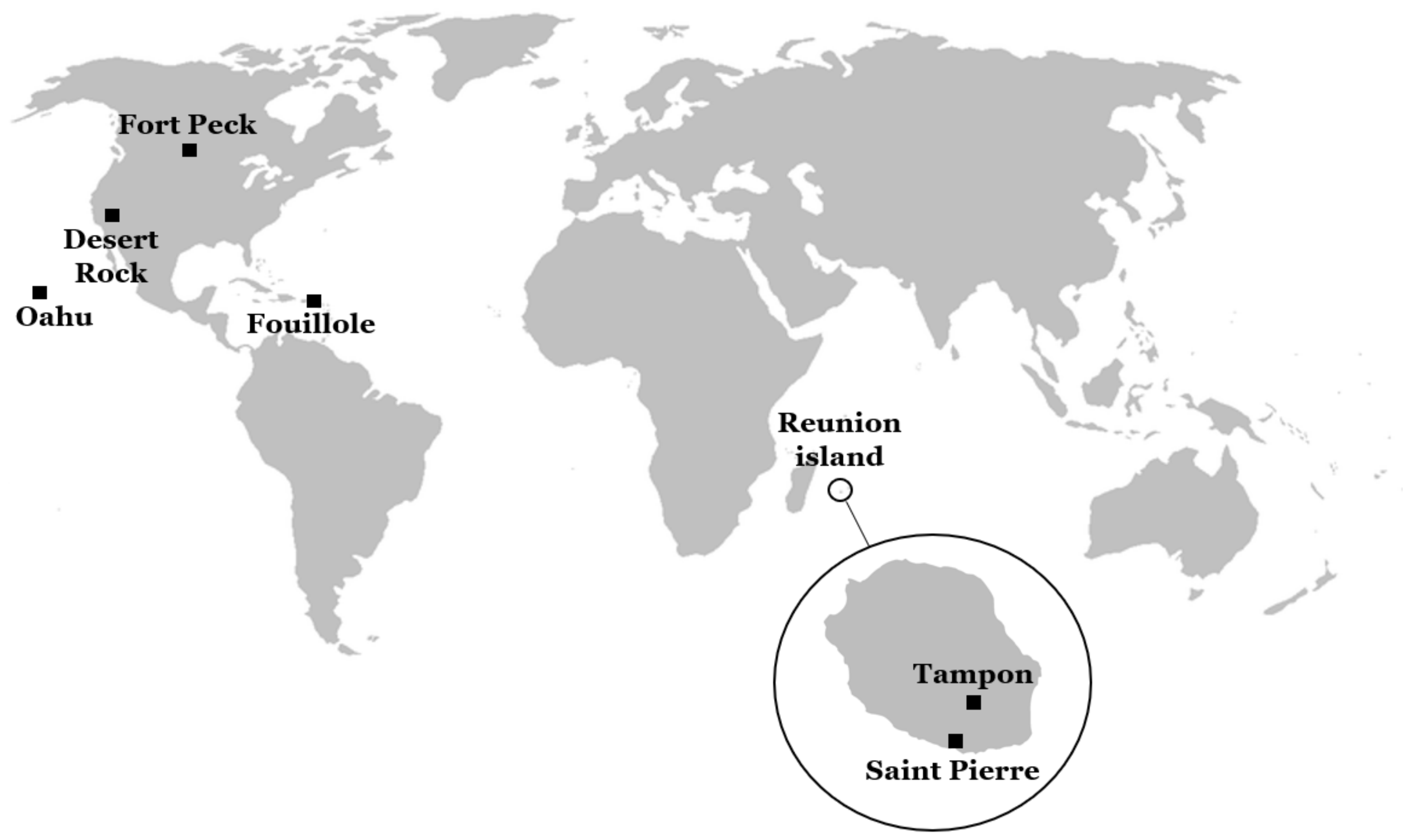
In this study, we used ground GHI data measured at six different sites around the world (see Figure 1).

Table 1. Site characteristics.

Site	Desert	Fort
Name	Rock	Peck	Oahu	Fouillole	St. Pierre	Tampon
code	DR	FP	OA	FO	SP	TA
provider	NOAA	NOAA	NREL	LARGE	PIMENT	PIMENT
latitude	36.6 N	48.3 N	21.3 N	16.6 N	21.3 S	21.3 S
longitude	119.0 W	105.1 W	158.1 W	61.5 W	55.5 E	55.5 E
elevation	1007 m	634 m	11 m	6 m	75 m	550 m
climate type	arid	continental	tropical	tropical	tropical	tropical
variability	0.1488	0.1852	0.2107	0.2115	0.1837	0.2326
training year	2012	2012	2010	2010	2012	2012
testing year	2013	2013	2011	2011	2013	2013
mean GHI of testing year (W/m${}^2$)	548	391	499	510	538	456

lists the six sites, which all experience different sky conditions. A specific preprocessing (data quality check and filtering) technique was applied to these data in previous works related to solar forecasting [13,14]. Because the focus here is to generate intra-day forecasts with a 1h time step, we computed the hourly average of GHI from the 1-min measurements at each location for two consecutive years. The first year for each location represents the training dataset, while the second year is the testing dataset. In keeping with a common practice in the realm of solar forecasting, it should be noted that all data have had solar elevation inferior to ${10}^{\circ }$ filtered out, hence removing nighttime, early morning, and late afternoon data.

2.2. Clear Sky Index

In the case of intra-hour or intra-day solar forecasts, time series-based forecasting techniques such as, for instance, autoRegressive (AR) linear techniques [15] are used to generate forecasts from past measurements of solar irradiance. A prerequisite of these linear time series technique is to work with stationary time series. Different degrees of stationarity are defined in the literature; a time series is said to be strictly stationary if the joint probability distribution F of the stochastic process is invariant under translation, while weak stationarity implies that the mean and the autocovariance do not depend on the time and that the second moment is finite [15]. More generally, stationarity means that the time series-related statistics such as the mean and the autocorrelation structure do not change over time [15].

Because the original GHI time series is not stationary (daily and annual cycles), it is common practice in solar forecasting to detrend the GHI time series using the output of a clear sky model. More precisely, a new detrended time series called a clear sky index $k_c$ time series is obtained using the following equation:

$$k_c=\frac{G_h}{G_{hc}},$$

(1)

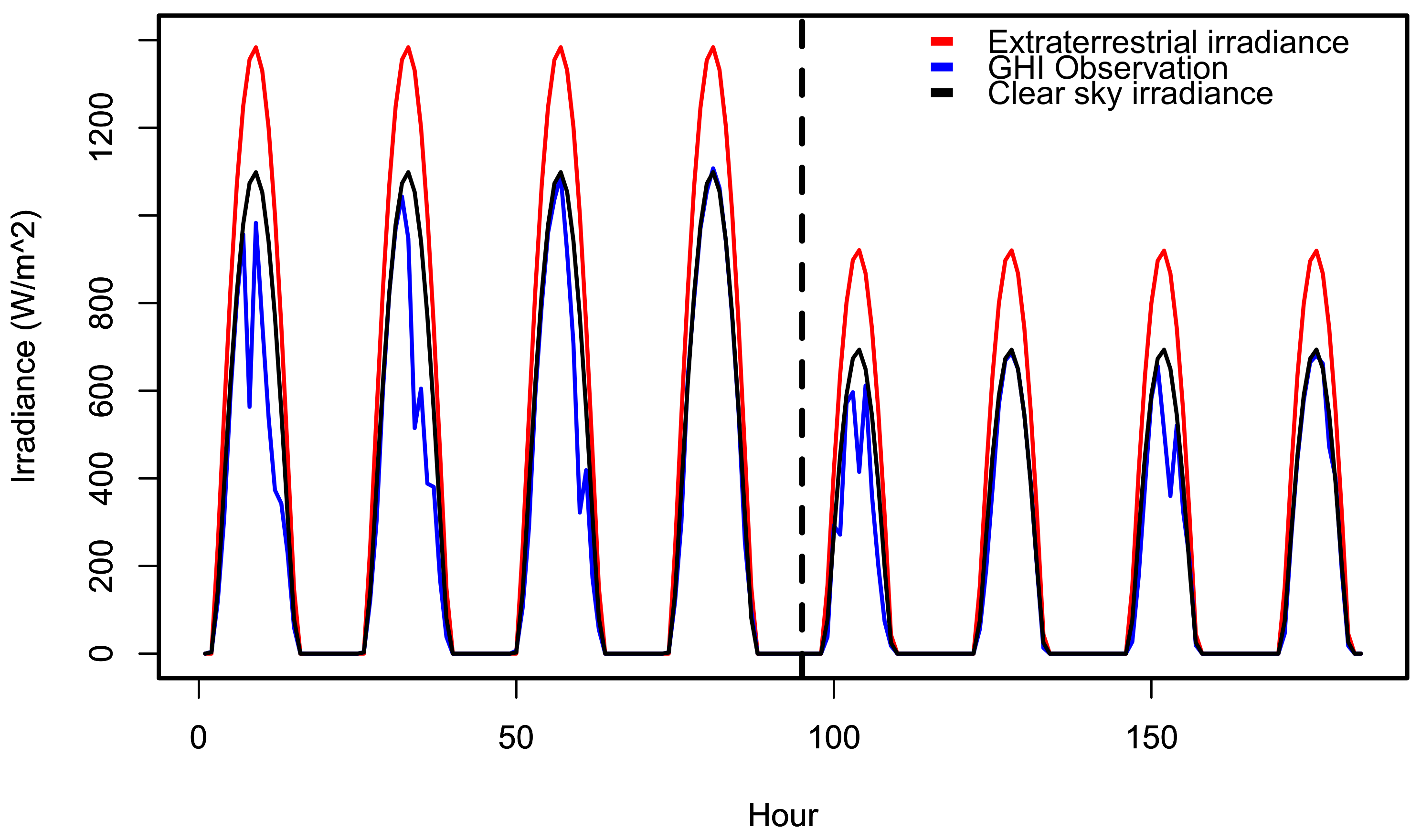
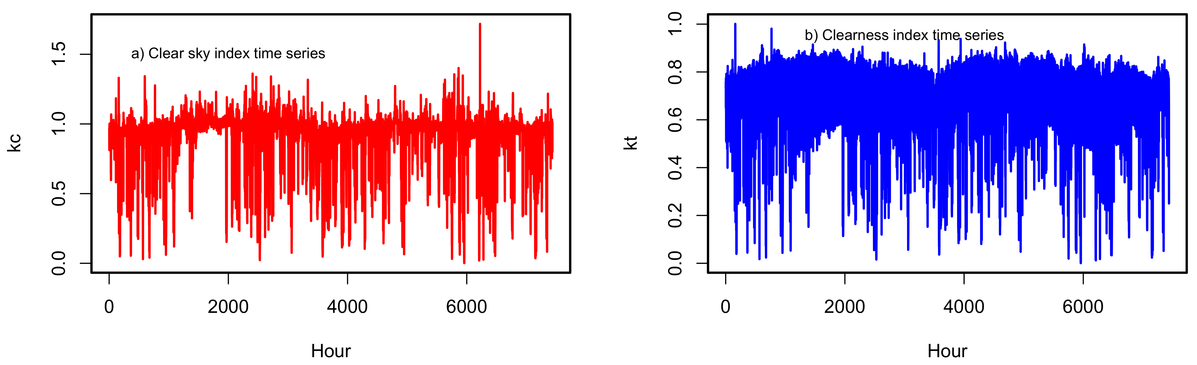
where $G_h$ is the measured global horizontal irradiance and $G_{hc}$ is the output of the specific clear sky model. As mentioned in Section 2.1, because the time step of the forecasts is 1h, we obtained hourly clear sky index time series by dividing the irradiance average of the hourly measurements with the hourly estimates of the clear sky model. Figure 2 shows eight days of measured GHI and the associated clear sky irradiances, while Figure 3a plots a clear sky index $k_c$ time series.

Equation (1) reveals that GHI can be considered as the product of a deterministic clear sky component and a stochastic cloud cover component, which is provided by $k_c$. With this approach, the construction of the forecasting models is based on the stochastic part of the global irradiance, while the deterministic part can be modeled by the clear sky model.

In this work, we used the clear sky values provided by the McClear model [2]. The CAMS website (Copernicus Atmosphere Monitoring Service, http://www.soda-pro.com, (accessed on 1 September 2022)) offers public McClear’s clear sky estimates with global coverage. Based on sophisticated radiative transfer computations and atmospheric parameters (aerosol, water vapor, and ozone data) provided by the CAMS service, the McClear model provides GHI clear sky values with good accuracy. However, it should be noted that uncertainty in atmospheric parameters can negatively impact the accuracy of a clear sky model [16,17,18]. Therefore, the availability and quality of atmospheric parameters are important for the choice of a specific clear sky model.

2.3. Clearness Index

Another way to remove the deterministic trends present in GHI time series is to use the extraterrestrial irradiance, i.e., the solar irradiance at a horizontal plane in the top of the atmosphere. GHI time series are normalized by dividing by the extraterrestrial irradiance, leading to the hourly clearness index $k_t$, written as

$$k_t=\frac{G_h}{G_{oh}}.$$

(2)

The hourly extraterrestrial average irradiance $G_{oh}$ on a horizontal surface for an hourly period is provided by [19]:

$$\begin{array}{cc}{G}_{oh}=\hfill & {\displaystyle \frac{12}{\pi }\times 1367\times \left[1+0.033cos\left(\frac{2\pi j}{365}\right)\right]\times \dots }\hfill \\ & {\displaystyle \left\{\frac{\pi ({\omega }_2-{\omega }_1)}{180}sin\left(\delta \right)sin\left(\varphi \right)+\left[sin\left(\frac{\pi {\omega }_2}{180}\right)-sin\left(\frac{\pi {\omega }_1}{180}\right)\right]cos\left(\delta \right)cos\left(\varphi \right)\right\}}\hfill \end{array}$$

(3)

where j is the Julian day, $\varphi$ is the latitude of the considered site, $\delta$ is the solar declination, and ${\omega }_1$ and ${\omega }_2$ are the hour angles in degrees at beginning and end, respectively, of the specific hour.

As defined by Equation (2), the clearness index has the ability to isolate the stochastic component in a global solar irradiance time series, similar to the clear sky index. Figure 2 shows examples of extraterrestrial irradiance, while Figure 3b plots a series of clearness indices. Both clear sky index (Figure 3a) and clearness index (Figure 3b) time series seem to exhibit changes in variance, possibly due to remaining seasonal variations. In other words, it appears that the two times series are not completely stationary, and are at least locally stationary. Appendix A provides a quantitative statistical analysis regarding the stationarity of these two time series.

2.4. Site Nominal Variability

Lauret et al. [20] showed that the site variability has an impact on the accuracy of solar forecasting methods. Therefore, in this study, we propose to assess the capability of the forecasting methods in relation to the site variability.

Table 1 provides the solar variability experienced by each site. In this study, the solar variability is defined as the standard deviation of the change in the clear sky index at a 1h time step [21], written as

$$\mathrm{Nominal}\mathrm{Variability}=\sigma (\Delta k_{c,\Delta t})=\sqrt{\mathrm{Var}(\Delta k_{c,\Delta t}}).$$

(4)

In this application, the time scale is $\Delta t=1\mathrm{hour}$. A site with a variability above $0.2$ is considered to experience variable sky conditions. As shown by Table 1, three sites, namely, OA, FO, and TA, exhibit high variability.

2.5. Forecasting Methods

2.5.1. Numerical Experiments Setup

In order to compare the $k_t$-approach against the $k_c$-approach, we selected a simple numerical setup in which the forecasting models must predict the next values of solar irradiance from only past values of the irradiance, i.e., no exogenous variables are used. In addition, in comparing the two approaches our aim was to select a simple linear technique such as an autoregressive (AR) process as well as a nonlinear one such as a neural network (NN) technique. Other nonlinear machine learning techniques (such as Support Vector machines or Gaussian processes) can be used as well; however, we selected the NN technique here, as it is often among the best performers [20].

Except for the persistence models described below, the two forecasting techniques described in this work, namely, the AR or the NN techniques, seek to find a generic model F in the form

$$\widehat{k}(t+h)=F\left(k\left(t\right),k(t-1)\cdots k(t-5)\right),$$

(5)

where $\widehat{k}(t+h)$ represents the predicted variable at a forecast horizon h that ranges from 1h to 6h (intra-day solar forecasting). The sequence $\left\{k\right(t),k(t-1)\cdots k(t-5\left)\right\}$ is the time series of the current and five past hourly values of either the clear sky index or the clearness index. Hence, here, the generic variable k may represent either the clear sky index $k_c$ or the clearness index $k_t$.

After the forecasts of the clear sky index or clearness index have been obtained, the corresponding indices can be transformed back to GHI forecasts using Equation (1) or Equation (2).

The statistical techniques used in this work are data-driven approaches. Consequently, the model parameters are estimated from N pairs of input and output samples contained in the training dataset. In a second step, after the models have been fitted, they are evaluated on the test dataset using the metrics provided in Section 2.6.

2.5.2. Persistence Model

In this work, we used two kinds of persistence model. The first is based on the clear sky index, and is provided by

$${\widehat{k}}_c(t+h)=k_c\left(t\right),$$

(6)

for all forecast horizons $h=1,2,\cdots ,6$.

The second uses the clearness index, and is defined by

$${\widehat{k}}_t(t+h)=k_t\left(t\right).$$

(7)

The persistence simply states the naive assumption that future values of the clear sky index or clearness index will remain equal to the clear sky index or clearness index observed at time t, i.e., the atmospheric conditions remain unchanged between the current time t and future time $t+h$. This way describing the persistence of the index instead of the GHI permits the sun path to be taken into account using either a clear sky model or the extraterrestrial irradiance. Recall that the corresponding GHI forecast can be obtained through either Equation (1) or Equation (2).

2.5.3. Linear AR Model

In an autoregressive (AR) model [15], the future value of a variable, that is, $\widehat{k}(t+h)$, is assumed to be a linear combination of several past observations, as shown by Equation (8):

$$\widehat{k}(t+h)={\mathrm{\Phi }}_0+\sum _{i=0}^p{\mathrm{\Phi }}_{i+1}k(t-i)+{ϵ}_t,$$

(8)

where ${ϵ}_t$ is white noise with variance ${\sigma }^2$, the model parameters are ${\left({\mathrm{\Phi }}_i\right)}_{i=0,1,\cdots ,p+1}$, and p is called the order (or autoregressive order) of the model. Following previous works [14,20], we select $p=5$, which corresponds to the current and past five measurements at a given time t.

2.5.4. Nonlinear NN Model

Artificial Neural Network (ANN or simply NN) is a technique capable of identifying a nonlinear relationship between input and output variables from the information contained in the training data set. A nonlinear mapping from an input vector x to an output y is obtained by an NN with d inputs, h hidden neurons, and a single linear output unit. The nonlinear relationship reads as

$$y=y(\mathbf{x},\mathbf{w})=\sum _{j=0}^h\left(w_{j}f\left(\sum _{i=0}^d{w}_{ji}{x}_i\right)\right).$$

(9)

The non-linear function f associated with h hidden units is usually the tangent hyperbolic function $f\left(x\right)=\frac{e^x-e^{-x}}{e^x+e^{-x}}$. The NN parameters, denoted by the parameter vector $\mathbf{w}=\{w_j,w_{ji}\}$, govern the nonlinear mapping and are adjusted during the training phase. The ability of the NN to generate correct predictions of unseen data is evaluated on the test dataset.

Assuming that the number of hidden neurons is sufficient, NNs are able to approximate any nonlinear continuous function at an arbitrary accuracy. However, if the NN has too many hidden neurons, inaccurate predictions are generated on the testing dataset. In the NN community, this issue is called overfitting. Several techniques, such as pruning or Bayesian regularization, can be employed to overcome overfitting problems. In this work, we used the Bayesian Technique to determine the optimal number of hidden nodes in the NN [22].

For our application, the relationship between the output $\widehat{k}(t+h)$ and the set of inputs $\left(k\left(t\right),k(t-1),\cdots ,k(t-5)\right)$ takes the form

$$\widehat{k}(t+h)=\sum _{j=0}^h\left(w_{j}f\left(\sum _{i=0}^p{w}_{ji}k(t-i)\right)\right).$$

(10)

As shown by the preceding equation, the NN model is equivalent to a nonlinear AR model for time series forecasting problems. In a similar manner, the number of past input values p is set to 5. Again, we stress that in Equations (8) and (10) the generic variable k can be either the clear sky index $k_c$ or the clearness index $k_t$. Finally,

Table 2. List of models used in this work.

Acronym	Comment
Pers kc	Persistence model based on the clear sky index
Pers kt	Persistence model based on the clearness index
AR kc	Linear Autoregressive model based on the clear sky index
AR kt	Linear Autoregressive model based on the clearness index
NN kc	Nonlinear Neural Network model based on the clear sky index
NN kt	Nonlinear Neural Network model based on the clearness index

lists the models implemented in this study.

2.6. Evaluation Metrics

In this work, and as suggested by a panel of solar forecasters [23], we employ the classical Root Mean Square Error (RMSE) metric. For N pairs of measurements/forecasts of GHI $\{G_h,{\widehat{G}}_h\}$, the RMSE read as

$$\mathrm{RMSE}=\sqrt{\frac{1}{N}{\displaystyle \sum _{i=1}^N}{\left({\widehat{G}}_h\left(i\right)-G_h\left(i\right)\right)}^2}.$$

(11)

It is a common practice to compute the relative Root Mean Square Error (rRMSE), which is obtained by dividing RMSE by the average of the daytime values of the GHI; see the last line of Table 1, which provides the observed mean GHI calculated for the testing year for each site. Recall that the rRMSE is negatively oriented, i.e., a lower value indicates that the model has better accuracy.

We propose evaluating the capability of the forecasting models against a baseline or reference model using the skill score (SS) [23], defined as

$$\mathrm{SS}=\left(1-\frac{{\mathrm{RMSE}}_{\mathrm{method}}}{{\mathrm{RMSE}}_{\mathrm{reference}}}\right)\times 100,$$

(12)

where ${\mathrm{RMSE}}_{\mathrm{method}}$ stands for the RMSE of each tested forecasting method and ${\mathrm{RMSE}}_{\mathrm{reference}}$ is the RMSE of the reference model.

The skill score is expressed as a percentage, and represents the relative accuracy improvement of the model over the reference model. With this definition, the reference model model has a forecast skill SS = 0%. Negative values of SS indicate that the new forecasting model fails to outperform the reference model, while positive values of SS mean that the forecasting method improves on the baseline model. Further, a higher the SS score indicates better improvement.

Here, as our aim is to evaluate the capability of the new forecasting models based on the clearness index, we compute skill scores with the three reference models based on the clear sky index, namely, the “Pers kc”, “AR kc”, and “NN kc” models. In other words, positive skill scores indicate which methods designed with the clearness index outperform their counterparts based on the clear sky index.

Finally, we stress here that the forecasting models generate GHI forecasts for each forecast horizon. Consequently, skill scores can be computed for each forecast horizon. As a way to sum up our results, we compute the average skill scores over all forecasting horizons, which leads to essentially the same conclusions with greater ease of visualization.

3. Results

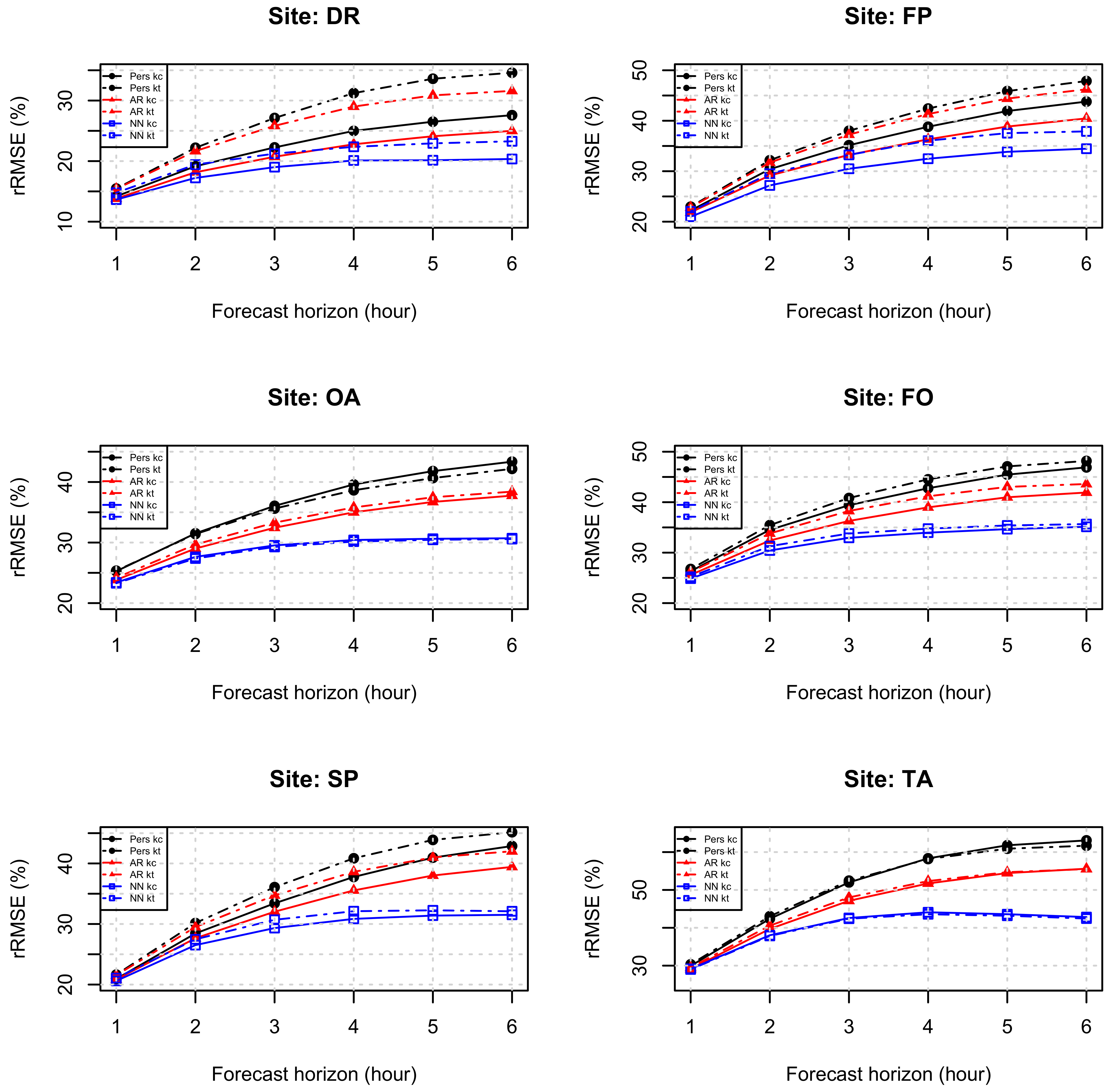
Figure 4 plots the relative RMSE metric in relation with the forecast horizon. As expected, irrespective of the site, the accuracy of all the models degrades with the forecast horizon. Furthermore, irrespective of forecasting technique it appears that the normalization of the data using a clear sky model leads to lower rRMSE (i.e., better accuracy) overall than normalization based on the extraterrestrial irradiance. However, the gap between the two approaches is reduced for sites experiencing a higher variability, such as OA, FO, and TA. In addition, it seems that this gap is reduced when using a nonlinear technique such as NN, which are able to obtain more information from the clearness index than the linear approach.

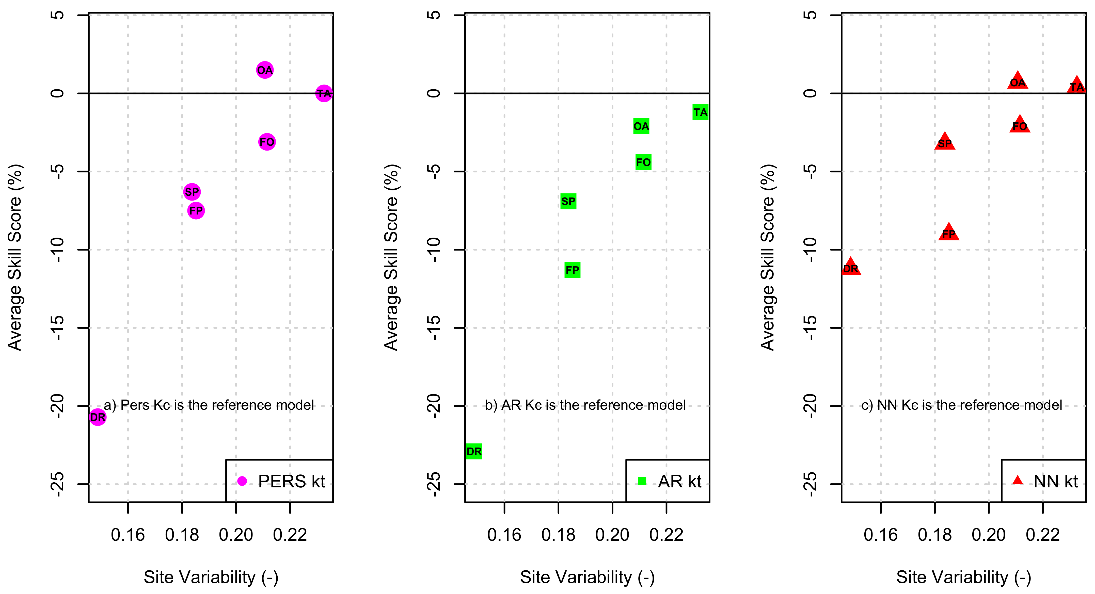
In order to better assess the relative merits of the $k_t$ approach, Figure 5 provides the average skill scores of the different forecasting models built from clearness time series vs. the three reference models designed with the clear sky index, namely, (a) “Pers kc”, (b) “AR kc”, and (c) “NN kc”. It can be observed that the forecasting skills of the clearness index-based approach are mostly negative, especially for those sites with hourly nominal variability lower than $0.2$. For sites with nominal variability above that limit, the results are not as conclusive. Indeed, the forecasting skill ranges between $\pm 3$%, that is, it is slightly positive in a few cases. This means that the use of the clearness index can lead to a competitive performance compared to the clear sky index only for high variability sites. For instance, the DR site (low variability) shows significantly negative skill when compared at same technique, with $-20$–22% persistence for AR model and of approximately $-10$% for the NN. For the SP and FP sites (nominal variability around $0.18$), the situation is the same, except with skill of $-11$–7% and $-9$–3%, respectively, showing that with higher variability there is a lower performance gap between the clear sky index and clearness index approaches, though with a clear advantage for the former in an event. Looking at the whole picture, i.e., a complete set of sites which exhibit different solar resource variability, it is clear that the use of the clear sky index should be preferred.

Finally, one interesting result pinpointed by Figure 5 is that there is a clear tendency for the average skill scores of the three “kt” models to increase with site variability.

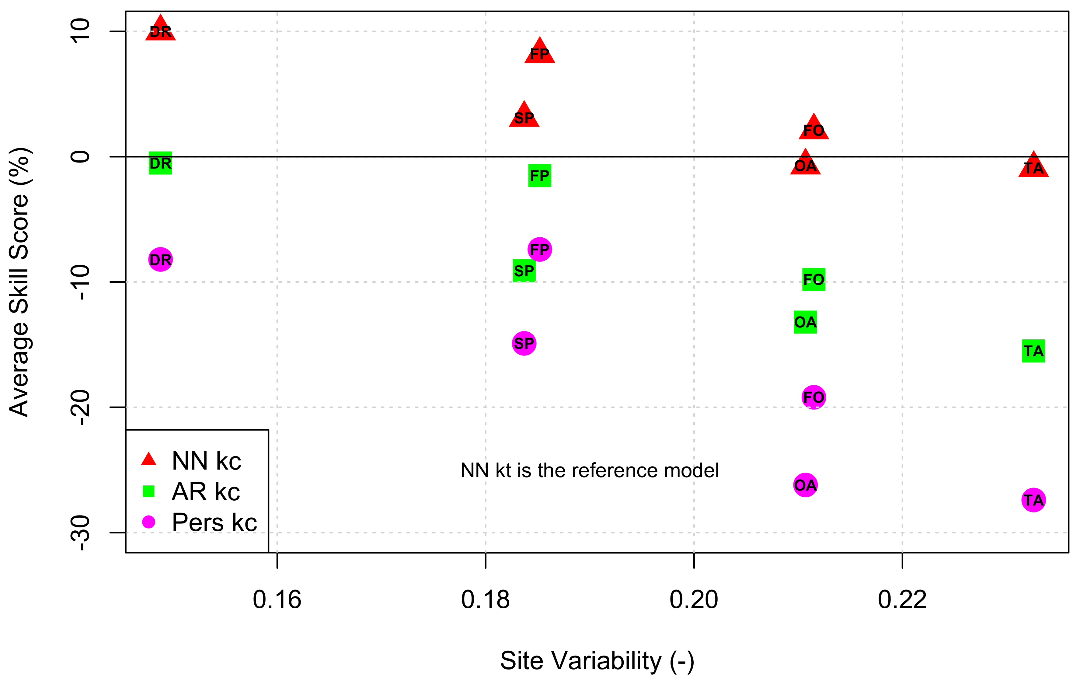
Lauret et al. [20] have shown that clear sky index-based forecasting models built with a nonlinear technique such as NN outperform linear and persistence approaches. In the following, we investigate whether an NN built with a time series of clearness indices can beat simple linear models built with the clear sky index, such as “Pers kc” or “AR kc”.

Figure 6 provides the average skill scores of the three models based on the $k_c$ approach when the reference model is the “NN kt” model. As shown by Figure 6, negative skill scores are obtained in the case of the “Pers kc” and “AR kc” models, indicating that the “NN kt” NN model built with a time series of clearness indices can outperform simple linear models such as “Pers kc” and “AR kc” built with the clear sky index. Conversely, it appears that the “NN kt” model cannot outperform the “NN kc”, model albeit positive or near zero skill scores are obtained for sites experiencing high variability such as FO, OA, and TA.

4. Discussion

Based on the above results, the following comments can be made. The use of the clear sky index is clearly a better option than the clearness index for building time-series forecasting models. This claim appears not as conclusive for special cases such as sites experiencing very high variability, for which the performances tends to be more balance across both options. The choice may further depend on the complexity of the forecasting methodology. In general, it seems that more complex techniques are able to obtain more information from the clearness index than simple baselines approaches, and therefore surpass its limitations to the point of being competitive with clear sky index-based models at high variability sites. In any case, apart from these special cases, which of course require further testing with worldwide solar irradiance datasets, the clear sky index should be preferred.

In addition, we have shown that the nonlinear NN $k_t$ approach outperforms the linear and persistence $k_c$ approaches. However, it may be difficult to build a nonlinear technique such as a neural network model. Indeed, this black-box approach can be very prone to overfitting. In other words, the gain in simplicity provided by the use of the clearness index compared to the complexity of nonlinear techniques may be a factor in choosing one method over the other.

In the case of sites with high variability (such as OA, FO, and TA in this study), it can be observed that a nonlinear technique such as NN generates similar predictions regardless of the type of normalisation used. This can be explained by the fact that such techniques do not require strong assumptions regarding the stationarity of the input time series. However, this observation must be confirmed by further study involving a larger number of sites.

More generally, the present study points out that a minimum quality of forecasting cannot be achieved if nonlinearity is avoided. If a forecaster wants to avoid complexity in preprocessing by choosing a $k_t$ approach, it is necessary to transfer the complexity to the forecasting technique itself in order to obtain a satisfactory minimum quality.

5. Conclusions

In this preliminary study, we have shown that normalization of the solar irradiance with the help of a clear sky model produces better forecasting models irrespective of the technique used. It appears, however, that a nonlinear forecasting technique such as a neural network built with clearness time series can outperform simple linear models constructed with the clear sky index. When the comparison is carried out with the same technique, the use of the clearness index is only competitive with that of the clear sky index for very high variability sites. In such cases, it seems that with the nonlinear technique, the clearness index approach can be relied on; however, nonlinear methods remain more complex, and therefore more difficult to optimize.

As we have stressed throughout this article, these results are preliminary and need to be confirmed by future studies selecting more sites with different weather conditions. Finally, we hope that this preliminary assessment will help to fill the gaps in the literature regarding the use of different forecasting methodologies based on the clearness index in the solar forecasting domain.

References

- Yang, D. Choice of clear-sky model in solar forecasting. J. Renew. Sustain. Energy 2020, 12, 026101. [Google Scholar] [CrossRef]
- Lefèvre, M.; Oumbe, A.; Blanc, P.; Espinar, B.; Gschwind, B.; Qu, Z.; Wald, L.; Schroedter-Homscheidt, M.; Hoyer-Klick, C.; Arola, A.; et al. McClear: A new model estimating downwelling solar radiation at ground level in clear-sky conditions. Atmos. Meas. Tech. 2013, 6, 2403–2418. [Google Scholar] [CrossRef]
- Skartveit, A.; Olseth, J.A.; Tuft, M.E. An hourly diffuse fraction model with correction for variability and surface albedo. Sol. Energy 1998, 63, 173–183. [Google Scholar] [CrossRef]
- Ridley, B.; Boland, J.; Lauret, P. Modelling of diffuse solar fraction with multiple predictors. Renew. Energy 2010, 35, 478–483. [Google Scholar] [CrossRef]
- Ruiz-Arias, J.; Alsamamra, H.; Tovar-Pescador, J.; Pozo-Vázquez, D. Proposal of a regressive model for the hourly diffuse solar radiation under all sky conditions. Energy Convers. Manag. 2010, 51, 881–893. [Google Scholar] [CrossRef]
- Engerer, N. Minute resolution estimates of the diffuse fraction of global irradiance for southeastern Australia. Sol. Energy 2015, 116, 215–237. [Google Scholar] [CrossRef]
- Gueymard, C.A.; Ruiz-Arias, J.A. Extensive worldwide validation and climate sensitivity analysis of direct irradiance predictions from 1-min global irradiance. Sol. Energy 2016, 128, 1–30. [Google Scholar] [CrossRef]
- Abal, G.; Aicardi, D.; Alonso-Suárez, R.; Laguarda, A. Performance of empirical models for diffuse fraction in Uruguay. Sol. Energy 2017, 141, 166–181. [Google Scholar] [CrossRef]
- Sanfilippo, A.; Martin-Pomares, L.; Mohandes, N.; Perez-Astudillo, D.; Bachour, D. An adaptive multi-modeling approach to solar nowcasting. Sol. Energy 2016, 125, 77–85. [Google Scholar] [CrossRef]
- Bracale, A.; Caramia, P.; Carpinelli, G.; Di Fazio, A.; Ferruzzi, G. A Bayesian Method for Short-Term Probabilistic Forecasting of Photovoltaic Generation in Smart Grid Operation and Control. Energies 2013, 6, 733–747. [Google Scholar] [CrossRef]
- Paulescu, M.; Paulescu, E.; Badescu, V. Nowcasting solar irradiance for effective solar power plants operation and smart grid management. In Predictive Modelling for Energy Management and Power Systems Engineering; Elsevier: Amsterdam, The Netherlands, 2021; pp. 249–270. [Google Scholar] [CrossRef]
- Antonanzas, J.; Osorio, N.; Escobar, R.; Urraca, R.; Martinez-de Pison, F.; Antonanzas-Torres, F. Review of photovoltaic power forecasting. Sol. Energy 2016, 136, 78–111. [Google Scholar] [CrossRef]
- David, M.; Luis, M.A.; Lauret, P. Comparison of intraday probabilistic forecasting of solar irradiance using only endogenous data. Int. J. Forecast. 2018, 34, 529–547. [Google Scholar] [CrossRef]
- Alonso-Suárez, R.; David, M.; Branco, V.; Lauret, P. Intra-day solar probabilistic forecasts including local short-term variability and satellite information. Renew. Energy 2020, 158, 554–573. [Google Scholar] [CrossRef]
- Chatfield, C. The Analysis of Time Series, 6th ed.; Chapman and Hall/CRC: New York, NY, USA, 2003. [Google Scholar] [CrossRef]
- Polo, J.; Antonanzas-Torres, F.; Vindel, J.; Ramirez, L. Sensitivity of satellite-based methods for deriving solar radiation to different choice of aerosol input and models. Renew. Energy 2014, 68, 785–792. [Google Scholar] [CrossRef]
- Zhong, X.; Kleissl, J. Clear sky irradiances using REST2 and MODIS. Sol. Energy 2015, 116, 144–164. [Google Scholar] [CrossRef]
- Gueymard, C.A. Chapter 5—Clear-Sky Radiation Models and Aerosol Effects. In Solar Resources Mapping: Fundamentals and Applications; Polo, J., Martín-Pomares, L., Sanfilippo, A., Eds.; Springer: Cham, Switzerland, 2019; pp. 137–182. [Google Scholar]
- Kalogirou, S.A. Environmental Characteristics. In Solar Energy Engineering; Elsevier: Amsterdam, The Netherlands, 2014; pp. 51–123. [Google Scholar] [CrossRef]
- Lauret, P.; Voyant, C.; Soubdhan, T.; David, M.; Poggi, P. A benchmarking of machine learning techniques for solar radiation forecasting in an insular context. Sol. Energy 2015, 112, 446–457. [Google Scholar] [CrossRef]
- Perez, R.; David, M.; Hoff, T.E.; Jamaly, M.; Kivalov, S.; Kleissl, J.; Lauret, P.; Perez, M. Spatial and Temporal Variability of Solar Energy. Found. Trends® Renew. Energy 2016, 1, 1–44. [Google Scholar] [CrossRef]
- MacKay, D.J.C. A Practical Bayesian Framework for Backpropagation Networks. Neural Comput. 1992, 4, 448–472. [Google Scholar] [CrossRef]
- Yang, D.; Alessandrini, S.; Antonanzas, J.; Antonanzas-Torres, F.; Badescu, V.; Beyer, H.G.; Blaga, R.; Boland, J.; Bright, J.M.; Coimbra, C.F.; et al. Verification of deterministic solar forecasts. Sol. Energy 2020, 210, 20–37. [Google Scholar] [CrossRef]
- Kwiatkowski, D.; Phillips, P.C.; Schmidt, P.; Shin, Y. Testing the null hypothesis of stationarity against the alternative of a unit root. J. Econom. 1992, 54, 159–178. [Google Scholar] [CrossRef]
- Said, S.E.; Dickey, D.A. Testing for unit roots in autoregressive-moving average models of unknown order. Biometrika 1984, 71, 599–607. [Google Scholar] [CrossRef]