Abstract
With the development of predictive management strategies for power distribution grids, reliable information on the expected photovoltaic power generation, which can be derived from forecasts of global horizontal irradiance (GHI), is needed. In recent years, machine learning techniques for GHI forecasting have proved to be superior to classical approaches. This work addresses the topic of multi-horizon forecasting of GHI using Gaussian process regression (GPR) and proposes an in-depth study on some open questions: should time or past GHI observations be chosen as input? What are the appropriate kernels in each case? Should the model be multi-horizon or horizon-specific? A comparison between time-based GPR models and observation-based GPR models is first made, along with a discussion on the best kernel to be chosen; a comparison between horizon-specific GPR models and multi-horizon GPR models is then conducted. The forecasting results obtained are also compared to those of the scaled persistence model. Four performance criteria and five forecast horizons (10 min, 1 h, 3 h, 5 h, and 24 h) are considered to thoroughly assess the forecasting results. It is observed that, when seeking multi-horizon models, using a quasiperiodic kernel and time as input is favored, while the best horizon-specific model uses an automatic relevance determination rational quadratic kernel and past GHI observations as input. Ultimately, the choice depends on the complexity and computational constraints of the application at hand.
1. Introduction
Over the past few years, the ever-growing energy demand jointly with the depletion of fossil fuels and environmental concerns have promoted the integration of renewable-energy-based power generation into power distribution grids. However, due to the fluctuating nature of renewable energy sources, particularly solar photovoltaics (PV), their higher penetration into power distribution grids poses significant challenges for grid operators [1,2]. Indeed, the deployment of distributed generation complicates the achievement of grid operators’ main goal of ensuring the power distribution grid balance at all times. The development of grid-connected PV power systems uncovers constraints [3], especially voltage fluctuations, mainly observed on low- and medium-voltage power distribution grids, and therefore makes the elaboration of smart management tools necessary. As a result, the development of predictive management strategies is required to ensure an efficient real-time monitoring and optimization of grid operation [4]. These strategies need reliable information on the expected PV power generation, which can be derived from forecasts of global horizontal irradiance (the total amount of shortwave radiation received from above by a horizontal surface on Earth, noted GHI hereafter). The work presented in this paper focuses on GHI forecasting, with forecast horizons ranging from 10 min to 24 h, thus including the intrahour, intraday and day-ahead cases that are useful for grid regulation, load-following production, power scheduling and unit commitment.
Solar irradiance forecasting is a milestone to relieve challenges aroused by the development of grid-connected PV power systems. Solar irradiance and PV power generation forecasting is an active field of research, and many approaches have been developed in the scientific literature [5,6]. Depending on the available data and the forecast horizons, different forecasting methods are adequate. Intrahour solar irradiance forecasts with a high spatial and temporal resolution may be provided by models using ground-based sky images [7,8,9]. For forecast horizons ranging from a few minutes to 6 h, statistical models with on-site solar irradiance observations as input are more suitable [10,11]. Additionally, cloud motion, provided by satellite images analysis, can be extrapolated to the upcoming few hours and allows to obtain good forecasts for forecast horizons up to 6 h [12,13]. However, techniques based on sky imagers or satellite images are very complex and involve many steps [14]. For forecast horizons from about 6 h onwards, accurate solar irradiance forecasts may be delivered by numerical weather prediction (NWP) models [15].
Although dynamic phenomena such as cloud motion, leading to unexpected changes in GHI, may not be anticipated by statistical models, they have been extensively used and have proven good performances for intrahour, intraday and even day-ahead solar irradiance and PV power generation forecasting [10,11,16,17]. Statistical models span from classical time-series approaches such as persistence models or autoregressive models [18,19] to machine learning techniques such as regression trees [19], k-nearest neighbors (kNN) [20], artificial neural networks (ANN) [11,21], support vector regression (SVR) [22] and Gaussian process regression (GPR) [11,23,24,25]. Combined or hybrid models involving different kinds of input data and/or methods to develop more precise forecasting models can also be found [26]. Since most classical time-series approaches are well-suited for stationary or quasi-stationary signals, GHI data, which are non-stationary mainly due to the presence of daily and seasonal periodic patterns, can be preprocessed using clearness or clear-sky indexes [9,27]. Because of their ability to capture complex relationships between inputs and outputs, artificial intelligence-based approaches, which can model the solar irradiance data without any specific preprocessing step, appear to be the best alternative to classical time-series approaches. As a result, artificial intelligence-based approaches have become prevalent in GHI and PV power generation forecasting studies, and many authors have shown that they outperform traditional time-series models [10,11,16,24].
In recent years, among machine learning techniques, the use of GPR for GHI forecasting has gained in popularity. Due to their flexible non-parametric kernel-based nature, GPR models are a powerful tool for time series modeling. Table 1 provides a list of recent solar irradiance and PV power generation forecasting studies including GPR models. As can be seen, past observations of the time series to be forecasted (whether clear-sky or clearness indexes, PV power generation or GHI) is a popular input choice, as it highlights correlations between data samples. However, as Gaussian processes can be defined over time [28], it is also possible to consider time as an input, allowing the construction of a kernel particularly adapted to GHI thanks to the a priori knowledge on its evolution over time [24,29]. The model input influences the choice of a kernel and therefore the GPR model’s performance (see Section 2.2). Note that some authors forecast clear-sky or clearness indexes instead of GHI. In this article, GHI is forecast directly, as it avoids the use of clear-sky models, thus making sure all errors come from the GPR model itself; moreover, the inductive biases are much stronger when using GHI instead of clear-sky or clearness indexes, allowing to incorporate much more a priori knowledge in the kernel. Finally, as can be seen in Table 1, some authors also use additional exogenous input data, such as pressure, relative humidity, etc. Since these data may not be always readily available, it has been decided to compare performance when only the variable of interest is measured.

Table 1.
Main recent studies including Gaussian process regression models. For the meaning of abbreviations, see the end of the paper.
As a result, an in-depth study on GHI forecasting using GPR models is carried out. The pending questions that this paper attempts to answer are the following.
- What input should be chosen, time or past GHI observations?
- For each of those inputs, what is most appropriate kernel?
- What are the advantages and disadvantages of multi-horizon GPR models and horizon-specific GPR models?
To do so, a comparison between time-based and observation-based GPR models is made. Note that a byproduct of using time as input is that the obtained models are naturally multi-horizon, since they can provide GHI forecasts at any forecast horizon [24]. For observation-based GPR models, however, either a specific model for each forecast horizon (developing horizon-specific models is common in the literature [10,16]) or multi-horizon forecasting models can be developed [11]. Thus, first, a comparison between multi-horizon models using time or past observations is made to determine the adequate input; then, the best multi-horizon models are compared to horizon-specific models. The persistence on the clear-sky index, also known as the scaled persistence model, is included in this study as the reference model. The models are developed using a GHI database covering two years, with a sampling time of 10 min and five forecast horizons considered (10 min, 1 h, 3 h, 5 h, and 24 h).
The rest of this paper is organized as follows: in Section 3, the data used to develop and validate the models included in this study are described. Section 2 gives a description of the scaled persistence model and the GPR models used to forecast GHI. The forecasting results, as well as the criteria used to evaluate the models’ forecasting accuracy, are presented and discussed in Section 4. The paper ends with a conclusion.
2. Description of the Forecasting Models Included in This Study
This section describes the GHI forecasting models included in this study. The models’ implementation has been realized on a machine having an Intel® Xeon® CPU E7-4890 v2 @ 2.80 GHz. The Gaussian Processes for Machine Learning (GPML) Matlab toolbox [28] was used for the GPR models’ implementation.
2.1. Scaled Persistence Model
The persistence model considers that the forecasted GHI at a desired forecast horizon is equal to the observed GHI at the current time:
where GHI is the observed GHI, is the forecast, is the time step (here 10 min) and is the forecast horizon.
This simple model finds its limits when the solar irradiance is highly variable over the considered forecast horizon. A part of this variability comes from the apparent movement of the Sun. As this motion is precisely known, it is possible to correct its effect by using a clear-sky model. This gives rise to an improved version of the persistence model named persistence on the clear-sky index, also known as the scaled persistence model. The latter has become the reference model in GHI forecasting studies [10,11,33]. The GHI forecasted by the scaled persistence model at a forecast horizon is given by:
where is the GHI given by a clear-sky model.
A clear-sky model provides an estimation of the solar irradiance for a cloudless sky. A wide range of clear-sky models can be found in the scientific literature, involving many parameters such as site altitude, solar elevation angle, aerosol concentration, water vapor and various atmospheric parameters (see [34] for a thorough review of most existing clear-sky models). In the present paper, the approach used in [35] to develop a clear-sky direct normal irradiance (DNI) model is adapted to GHI to obtain a clear-sky GHI model. This approach combines the well-known Ineichen and Perez’s clear-sky model [36] with a persistence on atmospheric turbidity and has led to a very accurate clear-sky DNI model [35]. The adaptation of this model results in the following equation for the clear-sky GHI appearing in Equation (2):
where:
- t is the time;
- is the solar zenith angle;
- is the extraterrestrial solar irradiance: the solar irradiance incident on the outer limit of the Earth’s atmosphere, considering the whole solar spectrum;
- m is the relative optical air mass, defined as the ratio of the optical path length of the solar beam through the atmosphere to the optical path through a standard atmosphere at sea level with the Sun at the zenith; it is calculated here by the Kasten and Young’s formula [37], widely used by the scientific community:where , and .
- is the Linke turbidity coefficient [38], defined as the number of atmospheres without aerosols or water vapor necessary to produce the observed attenuation of the solar extraterrestrial irradiance;
- , , , and are parameters given by:where h is the altitude of the studied site.
For details on this approach, the reader is referred to [35].
2.2. Gaussian Processes
This section defines Gaussian processes (GP) and kernels used to model and forecast GHI. The kernel is a key element of GPR models and deeply influences their performance [24]. This section also exposes the underlying reasons behind the kernels chosen in this paper.
2.2.1. Definition
A Gaussian process is defined as a collection of random variables, any finite number of which have a joint Gaussian distribution [28]. It defines a prior distribution over functions that, in light of some observed data, can be updated to a posterior distribution over functions. In the same way that a Gaussian distribution is fully determined by its mean and covariance, a GP is completely defined by a mean function and a covariance function. Firstly introduced in the field of machine learning as the limiting case of Bayesian inference performed on artificial neural networks with an infinite number of hidden neurons [39], Gaussian processes have become a powerful tool for modeling and forecasting [28]. A function f distributed as a Gaussian process is denoted as , where and are arbitrary input variables, is the mean function, and is the covariance function, also called the kernel. For simplicity, and since the kernel is generally sufficient to encode assumptions about the function to be learned, the prior mean function is usually set to zero.
A kernel contains assumptions about the underlying function to be learned and assesses the similarity between the function values at different input points and [28]. Its choice has a significant impact on the performance of a GPR model [24]. Therefore, the selection of a suitable kernel requires great attention. Any function that leads to a positive semidefinite covariance matrix can be used as a valid covariance function. The readers are referred to [28] for more details and a complete list of basic covariance functions. Furthermore, kernels are closed under operations such as addition and multiplication, allowing to combine basic kernels to create rich and interpretable covariance functions [40].
2.2.2. Gaussian Process Regression
Let us consider the standard linear regression model with additive noise:
where is the input vector, y is the output, is additive white Gaussian noise with variance , and f is the regression function, supposed to be a Gaussian process. To forecast GHI using GPR with only endogenous data, one can either use time (one-dimensional, ) or past observations (multidimensional, ) as input.
GPR is a Bayesian non-parametric approach that aims to approximate the function f using a training dataset of n samples , where is the input matrix and is the vector of corresponding GHI values [28]. When the input is time, is of dimension , and each sample is a scalar value, while when past GHI observations are used as input, the dimension of is , and each sample is a D-dimensional vector.
In addition to GHI forecasts, 95% confidence intervals can be derived from the predictive distribution provided by GPR models. They are computed as follows:
where CI are confidence interval bounds, is the mean prediction, and is the predictive variance given by the GPR model. For details on how the predictive distribution is obtained, the reader is referred to [28] (p. 16).
2.2.3. Training a GPR Model
A GPR model has hyperparameters that group the kernel’s parameters and the noise variance. These hyperparameters, denoted , have to be inferred from the training data. In practice, their estimation is commonly done by maximizing the log marginal likelihood, given by:
where is the Gram matrix, whose entries are , and is the identity matrix. Unfortunately, the function is usually non-convex with respect to hyperparameters. The problem space can have many local optima and the optimized hyperparameters depend on their initialization [40]. A common approach to deal with this drawback is to use various starting points randomly selected from an adequate prior distribution. In [41], the impact of initial hyperparameter priors on GPR models was studied, and the authors concluded that simple priors such as the uniform distribution in an appropriate range may be sufficient.
2.2.4. Kernels Used with Time-Based GPR Models
In [24,29,42], it was shown that when time is used as input of GPR models, the quasiperiodic kernel , obtained by multiplying the rational quadratic kernel and the periodic kernel , is the most suitable for multi-horizon GHI forecasting. These kernels are given by:
where is the amplitude, ℓ is the correlation length, determines the relative weighting of multi-scale variations and P is the period. The periodic kernel models functions with a global repetitive structure, and the rational quadratic kernel models functions that vary smoothly across many length-scales. The quasiperiodic kernel is then given by:
where and are correlation lengths.
The properties of GHI have led to this kernel composition. Indeed, as can be seen in Figure 1, over time, GHI exhibits a daily periodic pattern (due to solar geometry) modeled by the periodic kernel and a stochastic pattern (due to atmospheric conditions) modeled by the rational quadratic kernel.
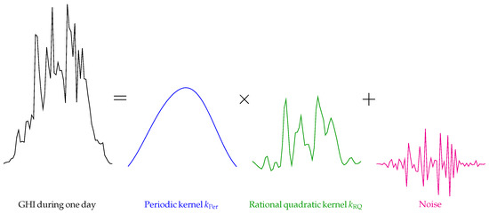
Figure 1.
GHI decomposition during one day: the periodic pattern is modeled by the periodic kernel and the stochastic pattern is modeled by the rational quadratic kernel.
Note that time-based GPR models are naturally multi-horizon forecasting models: since their input is the time, it suffices to provide the model with a date to obtain the desired forecast. The same model can thus provide GHI forecasts at any forecast horizon. Figure 2 shows a graphical view of GHI forecasting by the time-based GPR model with kernel . For the initialization of this model’s hyperparameters, the following choices were made:
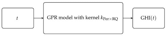
Figure 2.
Time-based GPR model with kernel .
- The hyperparameter was initialized to the variance of the training data;
- The period P was set to a day, indicating the daily periodicity of GHI;
- The remaining hyperparameters were randomly drawn from an uniform distribution .
The inspection of GHI data covering several years reveals the existence of a seasonal pattern (Figure 3) that can be incorporated in the time-based GPR model with kernel by adding a second periodic kernel to the quasiperiodic kernel [29]. Therefore, when data covering several years are considered, a suitable kernel for GHI forecasting by GPR models using time as input is given by:
where and are amplitudes, , and are correlation lengths, and are periods, and characterizes the relative weighting of multi-scale variations.
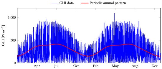
Figure 3.
GHI data covering years 2016 and 2017. A seasonal pattern appears when considering data over several years. Measurements taken at PROMES-CNRS laboratory in Perpignan.
A graphical view of GHI forecasting by the time-based GPR model with kernel is presented in Figure 4. The following choices were made for the initialization of this GPR model’s hyperparameters:
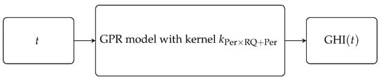
Figure 4.
Time-based GPR model with kernel .
- The hyperparameters and were initialized to the variance of the training data;
- The periods and were, respectively, set to one day and 365 days, indicating the daily and annual periodicity of GHI, respectively;
- The remaining hyperparameters were randomly drawn from a uniform distribution .
2.2.5. Kernels Used with Observation-Based GPR Models
In the case of GHI forecasting by GPR using past observations as input, authors have generally chosen kernels with isotropic length-scale [10,43]. Since the underlying function in this case has a multidimensional input variable and may not have the same variation level along each input dimension, anisotropic kernels (that can define an appropriate length-scale for each input dimension) are more suitable. Consequently, kernels with automatic relevance determination (ARD), which implicitly determine the relevancy of each input dimension, are used to model functions that have multidimensional input [11,40].
Contrary to time-based GPR models, observation-based GPR models are not naturally multi-horizon. One-step ahead forecasting models are very common in solar irradiance forecasting studies [10,16]: when a single horizon is needed, usually the data sampling time is changed to match the desired forecast horizon, but that downsampling can result in a serious simplification of GHI dynamics [11]. Multi-horizon forecasting models can then be obtained either by building a specific forecasting model for each horizon, which is demanding if many horizons are needed, or by iteratively performing one-step ahead forecasts until the desired horizons are obtained, which leads to the accumulation of forecast errors.
In this paper, the following ARD kernels are compared: the squared exponential kernel with ARD (), commonly selected by default; the rational quadratic kernel with ARD (); and the Matérn kernels with ARD (). They are, respectively, given by:
where is the amplitude, are correlation lengths along each input dimension and characterizes the relative weighting of large-scale and small-scale variations.
Figure 5 and Figure 6, respectively, show graphical views of GHI forecasting by multi-horizon and horizon-specific GPR models with kernel . For the hyperparameters’ initialization, the following choice have been made: is initialized to the variance of the training data, and the remaining hyperparameters are randomly drawn from a uniform distribution .
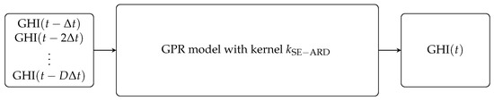
Figure 5.
Observation-based one-step-ahead GPR model with kernel , from which a multi-horizon model is obtained by iteration. is a vector of observations, and min is the time step.
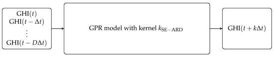
Figure 6.
Observation-based horizon-specific GPR model with kernel . , is a vector of observations, and min is the time step.
3. Description of Training and Test Datasets
The dataset used in this study derives from measurements taken at the laboratory PROMES-CNRS in Perpignan (southern France). The rotating shadowband irradiometer used to collect the measurements is a meteorological instrument composed of two horizontally leveled silicon photodiode radiation detectors placed in the center of a spherically curved shadowband. Its typical uncertainties are about . Located in the Occitania region near the Mediterranean Sea, Perpignan has a typical Mediterranean climate characterized by very hot summers and fairly mild winters. The region often experiences a north-west wind, the Tramontana, which keeps the sky clear much of the time.
Covering the years 2016 and 2017, the data are sampled at a min rate, resulting in around 26,600 points per year, after nights have been removed. The training dataset consists of the GHI measurements of the year 2016, and the test dataset consists of the GHI measurements of the year 2017. Figure 7 shows a map of data covering the two years.
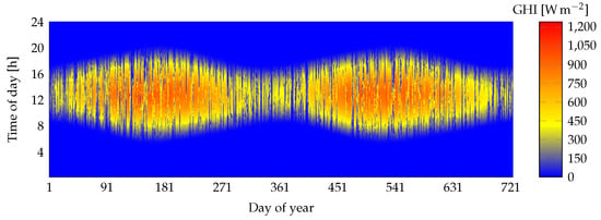
Figure 7.
GHI data covering years 2016 and 2017. Measurements are taken with a rotating shadowband irradiometer at PROMES-CNRS laboratory, located in Perpignan (southern France).
4. Results and Discussion
This section presents GHI forecasting results obtained using the scaled persistence model and the GPR models included in the study. The performance metrics used are also presented.
4.1. Performance Criteria
The models developed in this study are compared using the normalized root-mean-square error (nRMSE), the dynamic mean absolute error (DMAE), the interval score (IS) and the skill score (). These criteria are described below.
4.1.1. Normalized Root-Mean-Square Error
The nRMSE is a common evaluation metric adopted by the scientific community:
where is the test data and is the forecast. The nRMSE penalizes large deviations between forecasts and observations without quantifying errors due to temporal mismatches that may lead to over- or underestimation of events such as peaks or ramps.
4.1.2. Dynamic Mean Absolute Error
The DMAE [44,45] is used to simultaneously evaluate temporal mismatches and mean absolute error between forecasts and observations. The normalized mean absolute error (nMAE) is given by:
where is the test data, and is the forecast. The DMAE is computed by:
where is the normalized mean absolute error between forecasts and test data after shifting the time by a temporal distortion ranging from 0 to c (the maximum allowed temporal distortion), and determines the range of TDI values where their associated errors will be more penalized (here, and ). For details about this criterion, the reader is referred to [44,45].
4.1.3. Skill Score
As the nRMSE of a forecasting model depends on the atmospheric conditions of the considered site, it should be compared to the nRMSE of a reference model to demonstrate its accuracy. The skill score, denoted , is the criterion generally used to compare the performance of a model against a reference model [46]:
A positive SS score indicates that the developed model outperforms the reference model, which is chosen to be the scaled persistence model here.
4.1.4. Interval Score
The IS evaluates the forecast’s quality based on the associated confidence intervals [47]:
where is test data, is the lower bound of the confidence intervals, is the upper bound of the confidence intervals and , with the nominal value associated with the confidence intervals (here, , so ). This criterion rewards narrow confidence intervals and penalizes forecasts for which the observations are outside the confidence intervals.
4.2. Forecasting Results
This section compares GHI forecasts given by all the models included in this study:
- The scaled persistence model;
- The time-based multi-horizon GPR models, with kernels and ;
- The observation-based multi-horizon GPR models (obtained by iterating one-step-ahead forecasting models until the desired forecast horizon is reached), with kernels , , , , and ;
- The observation-based horizon-specific GPR models, with kernels , , , , and .
The models’ performance is evaluated using the above-mentioned criteria, which are computed for each model and each of the five considered forecast horizons (10 min, 1 h, 3 h, 5 h, and 24 h). It should be noted that at the lowest forecast horizon (10 min), there is no difference between the multi-horizon GPR models and the horizon-specific GPR models, since the multi-horizon forecasts are obtained by iterating one-step ahead forecasts.
In the sequel, a comparison between multi-horizon GPR models is made in Section 4.2.1, a comparison between mono- and multi-horizon GPR models is conducted in Section 4.2.2, and the contribution of the annual periodic kernel in time-based GPR models is studied in Section 4.2.3. The values of the performance criteria for these three cases are given in Figure 8, Figure 9 and Figure 10, respectively. In addition, further insight on the behavior of models and the influence of the kernels is given by Figure 11, Figure 12, Figure 13, Figure 14 and Figure 15: each of these figures presents an example of seven-day GHI forecasts (from 20 November 2017 to 26 November 2017) obtained with the scaled persistence model and all GPR models considered in this study at one of the five considered forecast horizons.
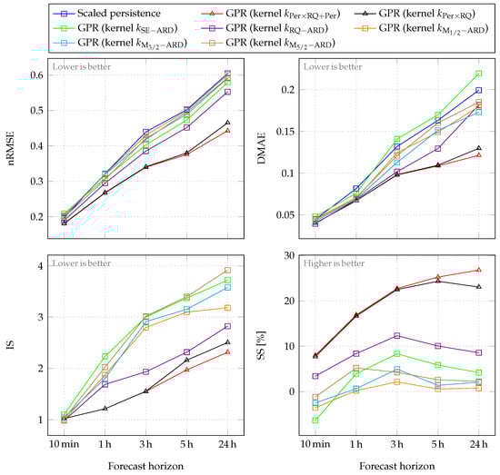
Figure 8.
Comparison between multi-horizon GPR models: performance criteria values for time-based (with triangular marks) and observation-based (with square marks) models. Note that the latter are obtained by iterating one-step-ahead models until the desired forecast horizon is reached. Values are calculated using test data (year 2017).
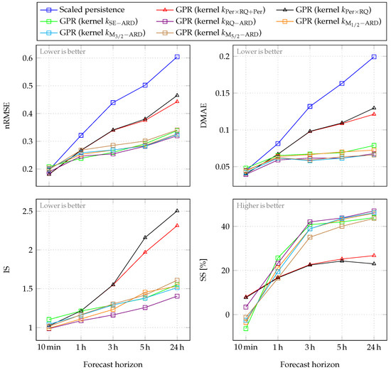
Figure 9.
Comparison between multi-horizon and horizon-specific models: performance criteria values for time-based GPR models (with triangular marks) and for observation-based horizon-specific GPR models (with square marks). Values are calculated using test data (year 2017).
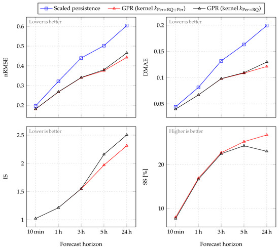
Figure 10.
Performance criteria values for time-based GPR models. Values are calculated considering test data (year 2017).
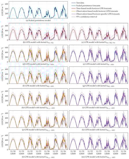
Figure 11.
Examples of 10 min GHI forecasts over one week, given by the scaled persistence model and the GPR models included in this study.
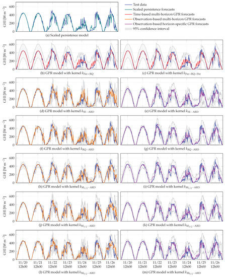
Figure 12.
Examples of 1 h GHI forecasts over one week, given by the scaled persistence model and the GPR models included in this study.
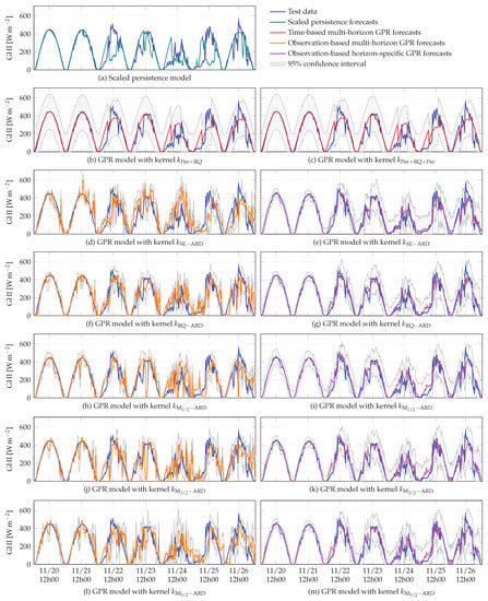
Figure 13.
Examples of 3 h GHI forecasts over one week, given by the scaled persistence model and the GPR models included in this study.
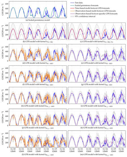
Figure 14.
Examples of 5 h GHI forecasts over one week, given by the scaled persistence model and the GPR models included in this study.
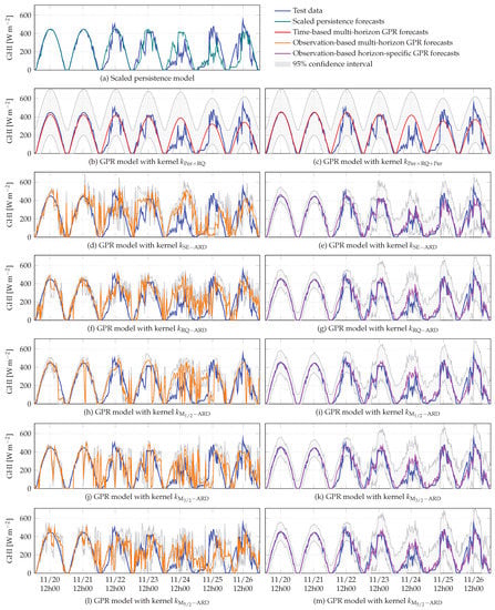
Figure 15.
Examples of 24 h GHI forecasts over one week, given by the scaled persistence model and the GPR models included in this study.
4.2.1. Multi-Horizon GPR Models: Time or Past Observations as Input?
In this section, multi-horizon GPR models using time as input are compared to those using past GHI observations. The values of performance criteria for these forecasting models are presented in Figure 8.
Let us first examine the 10 min forecast horizon. As can be noticed in Figure 8, all multi-horizon GPR models and the scaled persistence model give similar results. The persistence model, with , is even slightly more efficient than some GPR models, which confirms its efficiency for very short-term horizons. Nevertheless, the two GPR models using time as input have a slight advantage over all the others. These two models give similar results: for the GPR model with kernel and for the GPR model with kernel . We also observe similar results for all GPR models, depending on the interval score values, which evaluate the GHI forecast quality based on the associated confidence intervals. A large part of the test data falls within the confidence intervals associated with the forecasts given by the multi-horizon GPR models. Looking at the 10 min GHI forecast examples presented in Figure 11, the temporal evolutions of all forecasts are similar. It should be noted that the GPR model with kernel provides the worst results. This observation is confirmed by the performance criteria values. It can be deduced that this kernel, generally chosen by default, does not necessarily guarantee good results.
As the forecast horizon increases, the performance of all models degrades. There is a strong degradation in the scaled persistence model’s performance, which produces the worst results for all intraday forecast horizons (Figure 8). Although the basic persistence on GHI has been improved using a clear-sky model, as the forecast horizon increases its persistent nature becomes detrimental to the model. Furthermore, when the forecast horizon becomes longer, the accumulation of errors by iterating one-step-ahead forecasts affects the performance of observation-based multi-horizon GPR models. Among these models, the GPR model with kernel produces the best results. Concerning the time-based GPR models, their superiority over the other multi-horizon GPR models and the scaled persistence model becomes clear as the forecast horizon increases. When looking at the intraday forecasts given by observation-based multi-horizon GPR models (orange curves in Figure 11, Figure 12, Figure 13, Figure 14 and Figure 15), a strong degradation in performance is observed. This degradation is lessened for the two time-based GPR models (red curves in Figure 11, Figure 12, Figure 13, Figure 14 and Figure 15), as they produce periodic signals fitting to the GHI data. Indeed, as the forecast horizon increases, these models converge to the a priori knowledge on GHI, encoded in the chosen kernels. In Figure 11, Figure 12, Figure 13, Figure 14 and Figure 15, temporal shifts between the test data and the forecasts provided by the scaled persistence model are also observed, as well as between the test data and the forecast given by observation-based multi-horizon GPR model with kernel . These mismatches are reflected in the values of DMAE (Figure 8). Based on this criterion, the scaled persistence model and the observation-based multi-horizon GPR model with kernel produce the worst results for all the considered forecast horizons.
In our case, the forecasting models are developed for the implementation of a real-time model predictive control strategy, with a 10 min time step. At each time step, the controller needs forecasts ranging from 10 min to 24 h, which amounts to 144 forecast horizons. Now, if no approximation method is used, GHI forecasting by a GPR model requires the inversion of a matrix whose dimension is equal to the size of the training data. Thus, to obtain the forecasts, 144 matrices should be inverted at each time step when considering observation-based multi-horizon GPR models, while only one matrix should be inverted when considering time-based multi-horizon GPR models. The average execution time required to obtain a GHI forecast (that is, the forecast at the desired forecast horizon by time-based GPR models, or one iteration of the one-step-ahead forecast by observation-based GPR models) with the considered training data is about 12 s using a computational server equipped with an Intel® Xeon® E7-4890 v2 @ 2.80 GHz processor. As a result, time-based multi-horizon GPR models outperform observation-based multi-horizon GPR models while also having a lower computational cost.
However, instead of iteratively performing one-step-ahead forecasts, it is also possible to develop observation-based horizon-specific GPR models. In the following section, they are compared to time-based GPR models.
4.2.2. Multi-Horizon or Horizon-Specific GPR Models?
In this section, time-based GPR models are compared to observation-based horizon-specific GPR models. The performance criteria values for these models are presented in Figure 9.
As can be seen in Figure 9 and Figure 11, Figure 12, Figure 13, Figure 14 and Figure 15, observation-based horizon-specific GPR models are the best-performing, except at the 10 min forecast horizon, where the time-based GPR models outperform them slightly. Among observation-based horizon-specific GPR models, the GPR model with kernel produces marginally better results.
However, for our application (implementation of a real-time model predictive control strategy), to obtain GHI forecasts ranging from 10 min to 24 h, 144 horizon-specific GPR models should be developed, and it is still necessary to invert 144 matrices. These horizon-specific models thus generate quite a large computational cost that would hamper the real-time implementation of the strategy. Therefore, in this case, time-based multi-horizon GPR models are recommended. However, when few forecast horizons are considered or when there is no real-time implementation constraint, observation-based horizon-specific GPR models are recommended, since they give the best forecasting performance.
Through these comparative studies of time- and observation-based GPR models, it is noticed that time-based GPR models outperform observation-based multi-horizon GPR models and have a low computational cost compared to observation-based horizon-specific GPR models. Two time-based GPR models, with kernel and , have been developed. In the following section, the performance of these two models is compared to evaluate the contribution of the annual periodic kernel added to the quasiperiodic kernel .
4.2.3. Contribution of the Annual Periodic Kernel
The performance criteria values for these models are presented in Figure 10.
For a forecast horizon of 10 min, these two models give similar results and slightly outperform the scaled persistence model. These GPR models’ performance remains similar up to a forecast horizon of 3 h, but from 5 h onwards, we observe that the time-based GPR model with kernel provides better results. The inclusion of the seasonal component of the GHI becomes significant when the forecast horizon becomes longer. The slight superiority of the time-based GPR model with kernel for the considered forecast horizons indicates that the gain could be more important for forecast horizons of a few days or more. As the forecast horizon increases, the augmentation of IS values (Figure 10) of the time-based multi-horizon GPR models indicates the degradation of their performance. Nevertheless, among the time-based multi-horizon models, the GPR model with kernel produces the best results for all the considered forecast horizons. In Figure 15, for a 24 h horizon, the time-based GPR model with kernel fits the data better. The periodic kernel modeling the annual component of the GHI allows this model to produce a periodic signal with good long-term magnitude.
Note that without data to update the forecasts, a GPR model simply converges to its mean value learned during training. For a model based on a quasi-periodic kernel, this mean value is a periodic signal that could be interpreted as a sort of clear-sky model. Thus, for a forecast at a very long forecast horizon (a few months, for example), the time-based GPR model with kernel would have a great advantage, since its mean value also includes the annual periodic component of GHI.
5. Conclusions
In this paper, a comparative study of GPR models for GHI forecasting at intrahour, intraday and day-ahead forecast horizons is conducted. First, a study on which input between time and past GHI observations is conducted, along with a kernel study for each case. For observation-based GPR models, two categories of models are considered: multi-horizon forecasting models and horizon-specific forecasting models. The results of these models are compared to the results of time-based GPR models, which are naturally multi-horizon. The scaled persistence model is also included in this paper as the reference model. The models have been trained with one year of data and tested with another year of data, with a sampling time of 10 min.
According to the four performance criteria used, all the GPR models outperform the scaled persistence model, except at the lowest forecast horizon considered (10 min), where the scaled persistence model has an edge over a few of them. Regarding multi-horizon models, it is shown that, compared to observation-based GPR models, time-based GPR models have better forecasting performance, while also having a lower computational cost. Horizon-specific models using past GHI observations outperform all multi-horizon models. However, it should be noted that, depending on the application at hand, developing a model for each considered forecast horizon can be time and computationally demanding.
In the end, if multi-horizon models are needed, time-based GPR models and a quasiperiodic kernel should be chosen. When few forecast horizons are needed (or if time and computational constraints are low), observation-based horizon-specific GPR models and an automatic relevance determination rational quadratic kernel are advocated.
Author Contributions
Conceptualization, S.G. (Shab Gbémou), J.E., S.T. and S.G. (Stéphane Grieu); methodology, S.G. (Shab Gbémou), J.E., S.T. and S.G. (Stéphane Grieu); software, S.G. (Shab Gbémou), J.E., S.T. and S.G. (Stéphane Grieu); validation, S.G. (Shab Gbémou), J.E., S.T. and S.G. (Stéphane Grieu); formal analysis, S.G. (Shab Gbémou), J.E., S.T. and S.G. (Stéphane Grieu); investigation, S.G. (Shab Gbémou), J.E., S.T. and S.G. (Stéphane Grieu); resources, S.G. (Shab Gbémou), J.E., S.T. and S.G. (Stéphane Grieu); data curation, S.G. (Shab Gbémou), J.E., S.T. and S.G. (Stéphane Grieu); writing—original draft preparation, S.G. (Shab Gbémou), J.E., S.T. and S.G. (Stéphane Grieu); writing—review and editing, S.G. (Shab Gbémou), J.E., S.T. and S.G. (Stéphane Grieu); visualization, S.G. (Shab Gbémou), J.E., S.T. and S.G. (Stéphane Grieu); supervision, S.G. (Shab Gbémou), J.E., S.T. and S.G. (Stéphane Grieu); project administration, S.G. (Shab Gbémou), J.E., S.T. and S.G. (Stéphane Grieu); funding acquisition, S.G. (Shab Gbémou), J.E., S.T. and S.G. (Stéphane Grieu). All authors have read and agreed to the published version of the manuscript.
Funding
This research was co-funded by the Occitania Region (France) and the European Commission with the European Regional Development Funds (ERDF) under the Interreg SUDOE SOE3/P3/E0901 program (project IMPROVEMENT).
Institutional Review Board Statement
Not applicable.
Informed Consent Statement
Not applicable.
Data Availability Statement
Not applicable.
Conflicts of Interest
The authors declare no conflict of interest.
Abbreviations
The following abbreviations are used in this manuscript:
| ANN | Artificial neural network |
| ARD | Automatic relevance determination |
| CPU | Central processing unit |
| DMAE | Dynamic mean absolute error |
| DHI | Diffuse horizontal irradiance |
| DNI | Direct normal irradiance |
| GHI | Global horizontal irradiance |
| Clear-sky global horizontal irradiance | |
| GP | Gaussian process |
| GPML | Gaussian Processes for Machine Learning (Matlab toolbox) |
| GPR | Gaussian process regression |
| IS | Interval score |
| kNN | k-nearest neighbours |
| (n)MAE | (Normalised) mean absolute error |
| Matérn (kernel) of degree | |
| NWP | Numerical weather prediction |
| PV | Photovoltaic |
| Per | Periodic (kernel) |
| (n)RMSE | (Normalised) root mean square error |
| RQ | Rational quadratic (kernel) |
| SE | Squared exponential (kernel) |
| SS | Skill score |
| SVR | Support vector regression |
| UVA | Ultraviolet A |
| UVB | Ultraviolet B |
References
- Syranidou, C.; Linssen, J.; Stolten, D.; Robinius, M. Integration of Large-Scale Variable Renewable Energy Sources into the Future European Power System: On the Curtailment Challenge. Energies 2020, 13, 5490. [Google Scholar] [CrossRef]
- Erdiwansyah, M.; Husin, H.; Nasaruddin, M.Z.; Muhibbuddin. A critical review of the integration of renewable energy sources with various technologies. Prot. Control Mod. Power Syst. 2021, 6, 3. [Google Scholar] [CrossRef]
- ElNozahy, M.S.; Salama, M.M.A. Technical impacts of grid-connected photovoltaic systems on electrical networks—A review. J. Renew. Sustain. Energy 2013, 5, 032702. [Google Scholar] [CrossRef]
- Dkhili, N.; Eynard, J.; Thil, S.; Grieu, S. A survey of modelling and smart management tools for power grids with prolific distributed generation. Sustain. Energy Grids Netw. 2020, 21, 100284. [Google Scholar] [CrossRef]
- Sobri, S.; Koohi-Kamali, S.; Rahim, N.A. Solar photovoltaic generation forecasting methods: A review. Energy Convers. Manag. 2018, 156, 459–497. [Google Scholar] [CrossRef]
- Mellit, A.; Massi Pavan, A.; Ogliari, E.; Leva, S.; Lughi, V. Advanced Methods for Photovoltaic Output Power Forecasting: A Review. Appl. Sci. 2020, 10, 487. [Google Scholar] [CrossRef]
- Chu, Y.; Pedro, H.T.C.; Li, M.; Coimbra, C.F.M. Real-time forecasting of solar irradiance ramps with smart image processing. Sol. Energy 2015, 114, 91–104. [Google Scholar] [CrossRef]
- Schmidt, T.; Kalisch, J.; Lorenz, E.; Heinemann, D. Evaluating the spatio-temporal performance of sky-imager-based solar irradiance analysis and forecasts. Atmos. Chem. Phys. 2016, 16, 3399–3412. [Google Scholar] [CrossRef]
- Nou, J.; Chauvin, R.; Eynard, J.; Thil, S.; Grieu, S. Towards the intrahour forecasting of direct normal irradiance using sky-imaging data. Heliyon 2018, 4, e00598. [Google Scholar] [CrossRef]
- Lauret, P.; Voyant, C.; Soubdhan, T.; David, M.; Poggi, P. A benchmarking of machine learning techniques for solar radiation forecasting in an insular context. Sol. Energy 2015, 112, 446–457. [Google Scholar] [CrossRef]
- Gbémou, S.; Eynard, J.; Thil, S.; Guillot, E.; Grieu, S. A Comparative Study of Machine Learning-Based Methods for Global Horizontal Irradiance Forecasting. Energies 2021, 14, 3192. [Google Scholar] [CrossRef]
- Wang, P.; van Westrhenen, R.; Meirink, J.F.; van der Veen, S.; Knap, W. Surface solar radiation forecasts by advecting cloud physical properties derived from Meteosat Second Generation observations. Sol. Energy 2019, 177, 47–58. [Google Scholar] [CrossRef]
- Kallio-Myers, V.; Riihelä, A.; Lahtinen, P.; Lindfors, A. Global horizontal irradiance forecast for Finland based on geostationary weather satellite data. Sol. Energy 2020, 198, 68–80. [Google Scholar] [CrossRef]
- Diagne, M.; David, M.; Lauret, P.; Boland, J.; Schmutz, N. Review of solar irradiance forecasting methods and a proposition for small-scale insular grids. Renew. Sustain. Energy Rev. 2013, 27, 65–76. [Google Scholar] [CrossRef]
- Mathiesen, P.; Collier, C.; Kleissl, J. A high-resolution, cloud-assimilating numerical weather prediction model for solar irradiance forecasting. Sol. Energy 2013, 92, 47–61. [Google Scholar] [CrossRef]
- Sharifzadeh, M.; Sikinioti-Lock, A.; Shah, N. Machine-learning methods for integrated renewable power generation: A comparative study of artificial neural networks, support vector regression, and Gaussian process regression. Renew. Sustain. Energy Rev. 2019, 108, 513–538. [Google Scholar] [CrossRef]
- Rajagukguk, R.A.; Ramadhan, R.A.A.; Lee, H.J. A Review on Deep Learning Models for Forecasting Time Series Data of Solar Irradiance and Photovoltaic Power. Energies 2020, 13, 6623. [Google Scholar] [CrossRef]
- Voyant, C.; Paoli, C.; Muselli, M.; Nivet, M.L. Multi-horizon solar radiation forecasting for Mediterranean locations using time series models. Renew. Sustain. Energy Rev. 2013, 28, 44–52. [Google Scholar] [CrossRef]
- Fouilloy, A.; Voyant, C.; Notton, G.; Motte, F.; Paoli, C.; Nivet, M.L.; Guillot, E.; Duchaud, J.L. Solar irradiation prediction with machine learning: Forecasting models selection method depending on weather variability. Energy 2018, 165, 620–629. [Google Scholar] [CrossRef]
- Pedro, H.T.C.; Coimbra, C.F.M. Nearest-neighbor methodology for prediction of intra-hour global horizontal and direct normal irradiances. Renew. Energy 2015, 80, 770–782. [Google Scholar] [CrossRef]
- Benali, L.; Notton, G.; Fouilloy, A.; Voyant, C.; Dizene, R. Solar radiation forecasting using artificial neural network and random forest methods: Application to normal beam, horizontal diffuse and global components. Renew. Energy 2019, 132, 871–884. [Google Scholar] [CrossRef]
- Zendehboudi, A.; Baseer, M.A.; Saidur, R. Application of support vector machine models for forecasting solar and wind energy resources: A review. J. Clean. Prod. 2018, 199, 272–285. [Google Scholar] [CrossRef]
- Rohani, A.; Taki, M.; Abdollahpour, M. A novel soft computing model (Gaussian process regression with K-fold cross validation) for daily and monthly solar radiation forecasting (Part: I). Renew. Energy 2018, 115, 411–422. [Google Scholar] [CrossRef]
- Tolba, H.; Dkhili, N.; Nou, J.; Eynard, J.; Thil, S.; Grieu, S. Multi-Horizon Forecasting of Global Horizontal Irradiance Using Online Gaussian Process Regression: A Kernel Study. Energies 2020, 13, 4184. [Google Scholar] [CrossRef]
- Lubbe, F.; Maritz, J.; Harms, T. Evaluating the Potential of Gaussian Process Regression for Solar Radiation Forecasting: A Case Study. Energies 2020, 13, 5509. [Google Scholar] [CrossRef]
- Guermoui, M.; Melgani, F.; Gairaa, K.; Mekhalfi, M.L. A comprehensive review of hybrid models for solar radiation forecasting. J. Clean. Prod. 2020, 258, 120357. [Google Scholar] [CrossRef]
- Inman, R.H.; Pedro, H.T.C.; Coimbra, C.F.M. Solar forecasting methods for renewable energy integration. Prog. Energy Combust. Sci. 2013, 39, 535–576. [Google Scholar] [CrossRef]
- Rasmussen, C.E.; Williams, C.K.I. Gaussian Processes for Machine Learning; MIT Press: Cambridge, MA, USA, 2006. [Google Scholar]
- Gbémou, S.; Tolba, H.; Thil, S.; Grieu, S. Global horizontal irradiance forecasting using online sparse Gaussian process regression based on quasiperiodic kernels. In Proceedings of the 2019 IEEE International Conference on Environment and Electrical Engineering and 2019 IEEE Industrial and Commercial Power Systems Europe (EEEIC/ICPS Europe), Genova, Italy, 11–14 June 2019; pp. 1–6. [Google Scholar]
- Guermoui, M.; Gairaa, K.; Rabehi, A.; Djelloul, D.; Benkaciali, S. Estimation of the daily global solar radiation based on the Gaussian process regression methodology in the Saharan climate. Eur. Phys. J. Plus 2018, 133, 211. [Google Scholar] [CrossRef]
- Huang, C.; Zhang, Z.; Bensoussan, A. Forecasting of daily global solar radiation using wavelet transform-coupled Gaussian process regression: Case study in Spain. In Proceedings of the 2016 IEEE Innovative Smart Grid Technologies—Asia (ISGT-Asia), Melbourne, VIC, Australia, 28 November–1 December 2016; pp. 799–804. [Google Scholar] [CrossRef]
- Salcedo-Sanz, S.; Casanova-Mateo, C.; Muñoz-Marí, J.; Camps-Valls, G. Prediction of Daily Global Solar Irradiation Using Temporal Gaussian Processes. IEEE Geosci. Remote Sens. Lett. 2014, 11, 1936–1940. [Google Scholar] [CrossRef]
- Notton, G.; Voyant, C. Chapter 3—Forecasting of Intermittent Solar Energy Resource. In Advances in Renewable Energies and Power Technologies; Yahyaoui, I., Ed.; Elsevier: Amsterdam, The Netherlands, 2018; pp. 77–114. [Google Scholar] [CrossRef]
- Antonanzas-Torres, F.; Urraca, R.; Polo, J.; Perpiñán-Lamigueiro, O.; Escobar, R. Clear sky solar irradiance models: A review of seventy models. Renew. Sustain. Energy Rev. 2019, 107, 374–387. [Google Scholar] [CrossRef]
- Chauvin, R.; Nou, J.; Eynard, J.; Thil, S.; Grieu, S. A new approach to the real-time assessment and intraday forecasting of clear-sky direct normal irradiance. Sol. Energy 2018, 167, 35–51. [Google Scholar] [CrossRef]
- Ineichen, P.; Perez, R. A new airmass independent formulation for the Linke turbidity coefficient. Sol. Energy 2002, 73, 151–157. [Google Scholar] [CrossRef]
- Kasten, F.; Young, A.T. Revised optical air mass tables and approximation formula. Appl. Opt. 1989, 28, 4735–4738. [Google Scholar] [CrossRef] [PubMed]
- Linke, F. Transmisions-Koeffizient und Trübungsfaktor. Beiträge Zur Phys. Der Atmosphäre 1922, 10, 91–103. [Google Scholar]
- Neal, R.M. Bayesian Learning for Neural Networks; Lecture Notes in Statistics; Springer Science + Business Media: Berlin/Heidelberg, Germany, 1996. [Google Scholar]
- Duvenaud, D.; Lloyd, J.; Grosse, R.; Tenenbaum, J.; Zoubin, G. Structure Discovery in Nonparametric Regression through Compositional Kernel Search. In Proceedings of the 30th International Conference on Machine Learning, Atlanta, GA, USA, 17–19 June 2013; Dasgupta, S., McAllester, D., Eds.; PMLR: Atlanta, GA, USA, 2013; Volume 28, pp. 1166–1174. [Google Scholar]
- Chen, Z.; Wang, B. How priors of initial hyperparameters affect Gaussian process regression models. Neurocomputing 2018, 275, 1702–1710. [Google Scholar] [CrossRef]
- Tolba, H.; Dkhili, N.; Nou, J.; Eynard, J.; Thil, S.; Grieu, S. GHI forecasting using Gaussian process regression: Kernel study. IFAC-PapersOnLine 2019, 52, 455–460. [Google Scholar] [CrossRef]
- Voyant, C.; Notton, G.; Kalogirou, S.; Nivet, M.L.; Paoli, C.; Motte, F.; Fouilloy, A. Machine learning methods for solar radiation forecasting: A review. Renew. Energy 2017, 105, 569–582. [Google Scholar] [CrossRef]
- Frías-Paredes, L.; Mallor, F.; Gastón-Romeo, M.; León, T. Assessing energy forecasting inaccuracy by simultaneously considering temporal and absolute errors. Energy Convers. Manag. 2017, 142, 533–546. [Google Scholar] [CrossRef]
- Frías-Paredes, L.; Mallor, F.; Gastón-Romeo, M.; León, T. Dynamic mean absolute error as new measure for assessing forecasting errors. Energy Convers. Manag. 2018, 162, 176–188. [Google Scholar] [CrossRef]
- Yang, D. Making reference solar forecasts with climatology, persistence, and their optimal convex combination. Sol. Energy 2019, 193, 981–985. [Google Scholar] [CrossRef]
- Lauret, P.; David, M.; Pinson, P. Verification of solar irradiance probabilistic forecasts. Sol. Energy 2019, 194, 254–271. [Google Scholar] [CrossRef]
Publisher’s Note: MDPI stays neutral with regard to jurisdictional claims in published maps and institutional affiliations. |
© 2022 by the authors. Licensee MDPI, Basel, Switzerland. This article is an open access article distributed under the terms and conditions of the Creative Commons Attribution (CC BY) license (https://creativecommons.org/licenses/by/4.0/).