Abstract
Human pressure has caused river ecosystems to be severely damaged. To improve river ecosystems, “working with nature”, i.e., nature-based Solutions (NbS), should be supported. The purpose of this paper is to evaluate the effects of a specific NbS, i.e., floodplain restoration, which provides, among others, the ecosystem service of nutrient retention. For these, an in-depth time series analysis of different nutrients’ concentrations and water physiochemical parameters was performed to obtain Water Quality Indices (WQI), which were calculated along the river. To estimate water quality from remote sensing data and to generate water quality maps along the river, Sentinel-2 water products were validated against in situ data, and linear regression (LR), random forest (RF), and support vector regression (SVR) were trained with atmospherically corrected data for chlorophyll-a and TSM. The results show different outcomes in diverse floodplains in terms of improvement of the water quality downstream of the floodplains. RF demonstrated higher performance to model Chl-a, and LR demonstrated higher performance to model TSM. Based on this, we provide an insightful discussion about the benefits of NbS. These methodologies contribute to the evaluation of already existing NbS on the Danube River based on a quantitative analysis of the effects of floodplain ecosystems to water quality.
1. Introduction
1.1. Research Context
Nature-based solutions (NbS) are “actions which are inspired by, supported by or copied from nature”, that are potentially “energy and resource-efficient and resilient to change” [1]. NbS can solve water management problems, restore ecosystems, and increase sustainability [1,2,3]. An ecosystem is at the center of the NbS implementation areas.
Human pressures have caused river ecosystems to be seriously damaged in the entire world. Over the past 50 years, pollution, nutrient enrichments, dam constructions, and unsustainable exploitations have led to rivers’ deterioration. For example, the interruption of migratory routes of fish species by dam and weir constructions has led to a critical decrease of these fish species or even for their extinction [4]. One major cause of river ecosystems’ degradation is nutrient pollution. It is causing growth of dangerous algal blooms in new river locations, where they have different toxicity levels, and they are lasting for longer hours [5]. Agricultural practices, river modifications, bank erosions, and fertilizer applications have caused a huge increase in nutrient loads in rivers, mainly from nitrogen (N) and phosphorus (P) [5,6,7,8,9]. Nitrogen is present in waterways by the forms of nitrite (NO2), nitrate (NO3), ammonium (NH4+), and organic N; phosphorus is present as particulate P, and soluble reactive P (SRP).
A good example for an NbS dealing with the degradation of river ecosystems is floodplain restoration. Floodplains are a space alongside a watercourse, which are typically developed by deposition of solid particles in the course of floods of different magnitude [10,11], where water, nutrient, sediment, and organism exchanges are happening [12,13]. Flooding events, ranging from frequent and very low discharge events to less frequent and high discharge events, support the dynamics of the floodplain ecosystem and impact multiple biophysical features (e.g., hydro-morphological features and soil hydrology). Additionally, floodplains play an important role for the natural functioning of a river [14,15], and provide ecosystem functions and ecosystem services (ES), i.e., “the quantifiable or qualitative benefits of ecosystem functioning to the overall environment, including the products, services, and other benefits humans receive from natural, regulated, or otherwise perturbed ecosystems” [16]. One of the most important ES of floodplains is the transformation and retention of nutrients in river streams [17,18,19], identified by nitrate-N, total particulate P, the Water Quality Index (WQI), or concentrations of chlorophyll-a (Chl-a) and total suspended matter (TSM).
1.2. Background
Nitrate-N and total particulate P are the two primary forms of N and P in floodplain studies [20], and are retained by denitrification for N [21] and sedimentation for P [22].
WQI is generally used to assess the quality of both groundwater and surface water (e.g., rivers), and it is very important to compute when dealing with water resources management [23,24,25]. WQI consists of combining multiple natural parameters (e.g., nutrients in water concentration and water physiochemical parameters), and translate them efficiently into a single value, reflecting the quality of water.
Satellite remote sensing is an approach to retrieve water quality parameters such as Chl-a and TSM [26], which according to the Water Framework Directive (2000/60/EC) (WFD), are very important to monitor, since they are one of the lead parameters that described the trophic state of water, in addition to phytoplankton biomass [27,28,29] and water clarity [30]. One example of a satellite remote sensing tool is the MultiSpectral Instrument (MSI) onboard Sentinel-2 (S2), which has a high resolution of up to 10 m, and it has shown very good results in estimating the Chl-a and TSM concentrations in lakes [31]. For complex waterbodies, additional studies for atmospheric correction (AC) algorithms can be developed [32]. For this reason, the Copernicus Program developed an open source database for satellite imagery to improve monitoring [33] through modeling. In fact, modeling can be used to set up a relation between the radiometric values obtained from satellite images and the in situ measurements acquired in a matching date. These relationships can be sorted as empirical, semi-analytical, or based on machine learning (ML) [34], e.g., through multivariate linear regression (MLR), random forest (RF), support vector regression (SVR), or neuronal networks models. ML is considered a novel field of study, hence it is still not very efficient in water quality estimation, and it is very important to understand its behavior in remote sensing for a better estimation of inland water qualities [35].
1.3. Research Objective
To understand the effects of nutrient retention in potential floodplain restoration NbS, we investigated the situation of water quality along the Danube River in time and space, and analyzed the effects of already existing, i.e., active, floodplains. Estimating the actual effect of floodplains on the retention of nutrients is a laborious process, which requires a high amount of measured data and/or proper modeling. Therefore, with this study, we aim at observing nutrient retention on the Danube, by analyzing nitrate-N, total particulate P, WQI, Chl-a, and TSM, and estimating their changes along the Danube floodplains.
To reach this main goal, different sub-objectives were set:
- displaying the behavior of specific parameters with a temporal analysis of water quality with field data from 1996 to 2017;
- investigating particular changes of the water quality at the spatial level through all active floodplains along the Danube River;
- assessing the effect of floodplains’ nutrient retention and water quality improvement by means of time series analysis of nutrients, physiochemical parameters, and WQI;
- analyzing the relationship between the river discharge and river water quality through correlation analysis between the nutrients’ retention values and the river discharge, as well as between the water quality improvement and the river discharge.
Moreover, remote sensing-based ML models (MLR, RF, and SVR) were trained using field measurements and Sentinel-2 products, to investigate the situation of water quality using satellite imagery and to generate water quality maps, describing the situation of water quality through all active floodplains along the Danube River.
The Danube River was chosen in our study because nearly all the floodplains of the large rivers located in Central Europe (e.g., the Rhine, Elbe, Danube, and Oder) have suffered degradation due to agricultural activities, structural flood protection measures, dam constructions, and land-use changes (urbanization and transport infrastructure) [36,37,38,39].
2. Study Area
We investigated floodplains located along the Danube River (Table 1). The river originates in West Germany and its outlet is in the Black Sea. In total, 17 active floodplains within the Danube River Basin were selected as targets. These were derived within the Danube Floodplain Project (Figure 1), which defined active floodplains as inundated areas (hydraulically active) during a flood event with a return period of 100 years (HQ100), and identified them through a ratio factor between the widths of floodplain and river, a minimum threshold to the size, and hydraulic characteristics of the floodplain (e.g., flow paths, stages, and natural flow characteristics should be maintained) [40].

Table 1.
Floodplain keywords, locations, upstream and downstream gauging stations, morphometric data, and their restoration demand, as assessed according to the Danube Floodplain Project [40].

Figure 1.
The active floodplains (FP) of the Danube River used in this study.
This area is relevant since the Danube has lost 80% of its former floodplains due to anthropogenic influence [41]. To monitor water quality dynamics in the river, field data measurements were acquired from multiple stations located in the vicinity of each floodplain. To analyze changes in water quality before and after each floodplain, we classified these stations as “upstream” and “downstream”. The restoration demand of each floodplain was reported as estimated from the Danube Floodplain Project (https://www.interreg-danube.eu/approved-projects/danube-floodplain (accessed on 10 December 2021) [42], indicating the level of restoration needed of each floodplain to regain its maximum functionality (e.g., providing groundwater recharge, filtering contaminants, supporting habitats, or transporting nutrients) (Table 1).
3. Materials and Methods
3.1. Evolution of Water Quality in the Danube River
3.1.1. Field Data
Information on the active floodplains and their restoration demand were retrieved from the open-source GIS website (http://www.geo.u-szeged.hu/dfgis/ (accessed on 10 December 2021) which provides spatial results of the Danube Floodplain Project [43]. Field data were retrieved from the Danube River Basin Water Quality Database [44]. Field measurements of hydrological variables are provided together with concentrations of different nutrients and other water physiochemical parameters. The water parameters used are river discharge, concentrations of ammonium, chlorophyll-a, nitrates, total nitrogen, and total phosphorus, in addition to conductivity, dissolved oxygen, pH, and total suspended matter.
3.1.2. Time Series Analysis
To understand the evolution of water parameters, time series graphs for each active floodplain (upstream and downstream) were analyzed. The values were aggregated to monthly and yearly averages, and important flood events were highlighted in the respective time frame to better understand the influence of these extreme events on the respective floodplains [44]. Complete time series plots for all floodplains and water parameters are provided in Figures S1–S10. Time series values were used to compute the nutrient retention, calculate the WQI, and compute the water quality improvements between upstream and downstream locations in relation to each active floodplain of the Danube River.
3.1.3. Floodplains and Data Availability
Based on data availability for each floodplain, nutrient retention and WQI were computed. Among all the floodplains analyzed (Table 1), we calculated the nutrient retention for both nitrogen and phosphorus for floodplains FP1, FP2, FP3, FP9, and FP10. As for the WQI, this was calculated for floodplains FP2, FP3, FP6, FP7, FP8, FP9, and FP10.
3.1.4. Nutrient Retention
The evaluation of water quality can be achieved by monitoring nutrient concentrations, and especially the nutrients that can provide information on the river’s trophic status, such as nitrogen (N) and phosphorus (P). To evaluate the contribution of a river, or in our case, a floodplain, to the nutrient balance of a system, nutrient loads and improvement or deterioration of water quality should be monitored [45]. However, there are no methods to measure nutrient loads directly [46]. Computing in-stream nutrient loads depends on the availability of data for the corresponding nutrients, and it can be done by different calculation methods. In general, they are the product of the nutrient concentration and the river discharge value [46]. Nutrient retention in floodplains can be then calculated by subtracting the nutrient load exiting the floodplain from the nutrient load entering it. Still, uncertainties in computation must be considered, since previous studies showed that nutrient loads computed from continuous river discharges and monthly nutrient concentrations (as in our case) deviate by 25% from the true values [47]. These deviations are caused by missing nutrient concentration peaks due to low frequency measurements (one time per month) and can lead to under- or over-estimation [47].
In our study, we computed the nitrate-N retention, as it is the primary form of nitrogen [20] and the total phosphorus retention in the different active floodplains of the Danube River, using the values generated from the time series analysis. Generally, nutrient retention in floodplains is computed per unit area of floodplain. For this study, the major interest was in the effects of nutrient retention in the active floodplains along the Danube River and not in retention rate per unit area. Therefore, only retentions in terms of nutrient loads were computed.
3.1.5. Water Quality Index (WQI)
WQI is a simple and efficient method to monitor the quality status. To describe the effect of floodplains in river restoration, we calculated the WQI upstream and downstream of each floodplain, and the WQI improvement in each floodplain. The WQI was calculated using Equation (1), developed to assess river water quality by Rodriguez de Bascarán [48,49], and the water parameters generated as described in Section 3.1.2.:
where Ci represents a normalized assigned value (in percent) for each parameter value and Wi represents a weight for each parameter, ranging from 1 to 4, where 1 represents a minor importance for the ecological life and 3 represents a major importance.
Two of the parameters used in the calculation of the WQI developed by Rodriguez de Bascarán [48,49] are the Chemical Oxygen Demand (COD) and the Total Dissolved Solids (TDS). Since COD and TDS are not available in our dataset, COD was replaced by Chl-a because a significant positive correlation was shown between COD and Chl-a [50]. Additionally, TDS was replaced by TSM, since it is the only parameter describing the hardness quality of water in our data [30]. This decision was supported by previous studies where TSM was used in the calculation of the WQI [51,52].
3.1.6. Correlation with River Discharge
An active floodplain is a hydraulically active area inundated by flood event with return period of 100 years [44]. Since the aim of this study is to understand the nutrient retention effect in active floodplains, it was important to focus on the river discharge values leading to a floodplain being active. For this matter, a correlation analysis was conducted between the nutrient retention in floodplains and the river discharge values, in addition to another correlation analysis between the water quality improvement values (using the WQI improvement values) and the river discharge values. The analysis was done by calculating the Pearson’s correlation coefficient. This analysis was used to determine the relationship between the discharge values and the water quality.
3.2. Modeling Water Quality Dynamics with Remote Sensing
Different products available from remote sensing sensors can be used to monitor water quality parameters. We focused on Chl-a and TSM, and analyzed their concentrations. These two variables, considered important indicators for water environmental quality evaluation [53,54], can be monitored by remote sensing sensors since they are considered optically active components [55], and ready-to-use products are available from atmospherically corrected procedures. There are several studies showing that the capabilities of Sentinel-2 products are suitable to estimate Chl-a and TSM in water [31,54,55,56], but with some challenges in retrieving accurate data [32]. Sentinel-2 temporal (5 days) and spatial (10 m) resolutions contribute to consider this satellite as one the few suited to analyze a narrow water body as a river, but still wide enough as the Danube River. To evaluate the usefulness of available remote sensing products, we compared remotely derived Chl-a and TSM against field-measured parameters. To further model water quality changes in the river surface, atmospherically corrected remote sensing reflectance and several spectral-derived features were used as input features to supply ML algorithms, and produce further spatial and temporal analyses.
3.2.1. Field and Remote Sensing Data Comparison
The field measurement data for the Chl-a and TSM concentrations were retrieved from the Danube River Basin Water Quality Database by the International Commission for the Protection of the Danube River (ICPDR) [44]. The Copernicus Open Access Hub (https://scihub.copernicus.eu/ (accessed on 16 December 2021) was used to download cloud free Sentinel-2 S2 MSI Level-1C (L1C) data for the period 2014–2017 over the area of interest. An allowed period of a ±3 day difference between the S2 image and its corresponding in situ measurement was taken into consideration while matching up data [34]. Then, the images were processed using SNAP (v8.0.0.0), the open access toolbox for processing Sentinel missions. A standard atmospheric correction was applied to account for the scattered signal of the atmosphere, and retrieve remote sensing reflectance (RRS) to further modeling process [55,57]. The Level 1C data from Sentinel-2 was processed using the Case 2 Regional Coast Color (C2RCC) algorithm [57], which uses a large database of Chl-a and TSM concentrations trained with neural network, as well as using extreme ranges of scattering and absorption properties. The C2RCC processor is adequate for optically complex Case 2 waters (as the Danube River) which also retrieves layers of Chl-a and TSM concentrations [58]. These products are evaluated against available in situ data using conventional error metrics, such as the coefficient of determination (R2) and the Root Mean Squared Error (RSME).
3.2.2. Machine Learning Models
After C2RCC product validation, modeling was conducted by means of three ML algorithms, which were assembled and trained to estimate the Chl-a and TSM as targets. The input features were the remote sensing reflectance bands from C2RCC and further derived radio spectral features. MLR [59,60,61,62,63], RF [64,65,66], and the SVR [67,68,69] were considered since they are becoming standard algorithms in ML modeling of water quality [64]. All ML algorithms were implemented in Python 3.10.0 using the Scikit-Learn 1.0.2 library. Feature engineering was used to develop additional predictors to test more modeling scenarios [34,70,71,72]. The complete additional feature combinations were also tested in related research of remote sensing of inland waters [72].
To select the most adequate predictors, all the predictors were tested with the Pearson’s correlation against Chl-a and TSM. The highest correlated features were then selected as input for the algorithms. To tune algorithm hyperparameters, we used a Grid Search with predefined values. The final dataset of remote sensing reflectance and target parameters was divided into train and test splits and evaluated using a leave one out cross-validation (LOOCV) [35]. LOOCV is a specific case of a K-fold cross-validation where K equals N (the number of data points), which eliminates biases that a single split in the dataset may cause by using this technique. This method partitioned the dataset into K-fold of freely selected observations. Every model was trained for each of the K possible training-test splits, and the reported values for R2 and RMSE were the average of these K runs.
Finally, the model with the best error metrics values was chosen for estimating Chl-a and TSM over the surface of the Danube River to visualize spatial distributions based on specific dates and locations detected in the time series and WQI variations on each floodplain. The complete process which summarizes the methodology applied in this work is shown in Figure 2.

Figure 2.
Flowchart describing the methodology applied in this work.
4. Results
4.1. Results on Water Quality Index (WQI)
Results indicate, in general, that floodplains act positively by improving water quality in floodplains (Figure 3). We can notice an improvement in water quality between upstream and downstream for the majority of years in FP2, FP6, FP7, FP8, and FP9. Floodplain FP3 also shows an improvement in water quality for some years, however, it displays very little data. Floodplain FP10 acts quite the opposite to the other floodplains, as it does not show any improvement of water quality downstream of the floodplain in any year.

Figure 3.
WQI percentual improvement and river discharge time series in: (a) FP2; (b) FP3; (c) FP6; (d) FP7; (e) FP8; (f) FP9; (g) FP10.
The percentage of improvement of WQI is still conservative and is usually below 8% for the whole period of analysis, with exception to FP8, which shows improvements of up to 20% (in 2015). Similarly, a decrease in WQI reaches maximum 7% for all floodplains except for FP10, which displayed WQI reductions up to 11%.
4.2. Nitrogen and Phosphorus Retention
Average yearly retention values for nitrates and phosphorus are shown in Figure 4. It can be seen that both FP2 and FP10 retain nutrients, whereas neither FP3 nor FP9 promote retention. On the other hand, FP1 retains very small amounts of nitrate but does not fortify phosphorus retention in cases when the retention load is too large.

Figure 4.
Average yearly retention values of the analyzed floodplains (FP) for: (a) Nitrogen; (b) Phosphorus.
4.3. Water Quality Variations
By averaging the improvement and worsening results of WQI, it is possible to have an overall view of the water quality variations. Results of this exercise are shown in Figure 5. Except for FP10, all floodplains show an average annual water quality improvement downstream of the corresponding floodplain. It is also noticeable that the extreme cases for improvement and worsening are the FP8 and FP10, respectively.

Figure 5.
Average yearly water quality improvement of the analyzed floodplains (FP).
4.4. Water Quality and Correlation with River Discharge
Complete Pearson’s correlation plots between average yearly nutrient retention and river discharge, as well as correlation plots between water quality improvement and river discharge value are provided in Figures S11–S13. These plots determine the relationship between the discharge values and the water quality. They can also explain the different behaviors of floodplains towards improving the water quality.
4.5. Remote Sensing-Based Machine Learning Models
4.5.1. C2RCC Water Products’ Validation
Correlation between C2RCC and in situ measurements is displayed in Figure 6. Poor results for both Chl-a and TSM products are retrieved, particularly for Chl-a, for which an overestimation occurs in the range of 0–10 mg/L. TSM shows underestimation for almost all the range of the concentration but a slightly better correlation R2 = 0.19. These results justify further modeling using RRS and locally-tuned machine learning approaches in an effort to estimate accurately Chl-a and TSM.

Figure 6.
In situ validation for Case 2 Regional Coast Color (C2RCC) algorithm results with in situ measurements: (a) Chlorophyll-a (Chl-a); (b) Total Suspended Matter (TSM).
4.5.2. Machine Learning Modeling
After the tuning of hyperparameters, the feature engineering process and the LOOCV, average error metrics were calculated and the three models were compared against each other. Results for Chl-a and TSM are displayed in Table 2 and Table 3. Chl-a ML models perform better with better results for Random Forest R2 = 0.60 and RMSE = 5.90 against SVM (R2 = 0.57 and RMSE = 6.10). TSM ML models perform very poorly, and only LR reach an R2 > 0.10. We chose, therefore, RFR for further estimation of Chl-a and LR for TSM. We assumed, however, that for TSM, we would retrieve highly uncertain results due to the very weak performance of TSM models.
Table 2.
Machine learning models’ results for best runs of each algorithm for Chl-a estimation.
Table 3.
Machine learning models’ results for best runs of each algorithm for TSM estimation.
4.5.3. Water Quality Maps
The results of water quality from modeling over the surface of Danube River confirm the previous results from Figure 5. Chl-a spatial variations are shown in Figure 7 for FP2 (Figure 7a), FP6 and FP7 (Figure 7b), and FP8 (Figure 7c). The selected dates of the image acquisition to display spatial variations were based on the time series analysis and WQI analysis. Similarly, TSM spatial variations are shown in Figure 8. From Figure 7, it is visible that upstream regions of FP 2 show a higher concentration of Chl-a (up to 23–27 mg/L), and downstream region reduces its concentration (<=3 mg/L). Similar scenarios are visible in Figure 7b for FP6 and FP7, except for the region at the extreme East, where a plume with high Chl-a concentrations is visible (Figure 7b, downstream). In Figure 7c, a clear difference is visible between upstream and downstream concentrations as well.
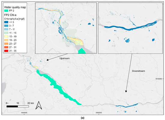

Figure 7.
Water quality maps for Chlorophyll-a expressed in mg/L for the three areas that correspond to (a) floodplain 2 (S2 image acquired on: 13 April 2016); (b) floodplains 6 and 7 (S2 image acquired on: 28 February 2017); (c) floodplain 8 (S2 image acquired on: upstream on 26 May 2017 and downstream on 15 May 2017). Basemap: ESRI Gray. EPSG: 3857.
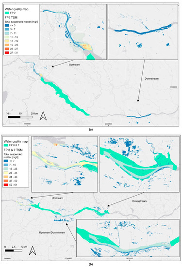

Figure 8.
Water quality maps for total suspended matter (TSM) expressed in mg/L for the three areas that correspond to (a) floodplain 2 (S2 image acquired on: 13 April 2016); (b) floodplains 6 and 7 (S2 image acquired on: 28 February 2017); (c) floodplain 8 (S2 image acquired on: upstream on 26 April 2017 and downstream on 15 May 2017). Basemap: ESRI Gray. EPSG: 3857.
5. Discussion
5.1. Water Quality and Nutrient Retention
Not all floodplains could be analyzed in our study since there was a lack of field measurements for important nutrients in some stations or an absence of discharge data in other stations.
Floodplains showing a positive behavior in improving the water quality downstream of the floodplain were described to have a low to medium restoration demand, showing that these floodplains’ functionality of filtering contaminants and improving water quality is active, and also, it can be improved further for FP6, FP7, FP8, and FP9, having a medium restoration demand. On the other hand, one floodplain (FP10) did not show a water quality improvement at any year, despite having a medium restoration demand. Still, it is possible that other functionalities are active in this floodplain, such as providing groundwater recharge or supporting habitats, but the improvement of water quality function is not active and needs to be restored.
Moreover, among the floodplains showing a pattern of retaining nutrients, we can notice that 83% of the years in which a flood occurred, the yearly average improvement of water quality was positive. This explains that during flooding years, the water quality improvement function of floodplains is more active.
Regarding the nutrient retention, only five floodplains had enough data to conduct the analysis. Some of the floodplains that showed a retention behavior in the general water quality analysis did not retain nutrients, and also acted quite poor in terms of nutrient retention and vice versa. This is due to other valuable parameters that are taken into consideration when computing water quality, such as Chl-a, TSM, and the Dissolved Oxygen concentrations. Therefore, sometimes, a floodplain may not serve for nutrient retention but it will improve other water quality parameters, leading to a better quality of water downstream.
The poor nutrient retention in floodplains can be caused by a release of nutrients greater than retention capacity. Sometimes, nutrient storages are not permanent due to the dynamic nature of floodplains. Some studies showed floodplains releasing nutrients or sometimes re-suspending them due to scouring currents occurring in the river. Other studies showed a net release of phosphorus or even an increase in both nitrogen and phosphorus amounts in the river channel next to a floodplain [73,74]. Additionally, in some cases, it is important to consider the presence of soluble reactive phosphorus (SRP), which can act disproportionally to downstream eutrophication [21]. Moreover, it is important to consider the nutrients that can be returned to the river via lateral stream migration and erosions from stream banks over long time periods, which can shrink the size of the floodplain each year as well [22,75].
Finally, it is very important to consider river discharge in floodplains because it is the river discharge values that determine the hydraulically connected area of an active floodplain [40]. The correlation between the water quality improvement or the nutrient retention and the river discharge values was not strong, except for some floodplains. In these floodplains, it is important to consider the hydraulic load and the water depth while designing flow rate recommendations for effective treatment, because they play critical roles in the effectiveness of nutrient removal [76]. The poor correlation between discharge rate and retention could be explained by a limited range on the available data and a small difference among inflow concentrations [77]. Finally, some floodplains showed a negative correlation, i.e., showing higher retentions during small river discharges. This can be explained by the fact that during low discharge periods, longer water residence times are expected, promoting nutrient retentions such as denitrification and other types of soil accumulation [78]. Additionally, we have to mention that some floodplains did not have enough sample points in order to do a significant correlation analysis. For example, FP3 and FP9 for both nitrates and phosphorus had only 5 sample points each, which is a small amount of data to make an accurate analysis.
5.2. Machine Learning Models Based on Remote Sensing
Modeling water quality parameters over inland waters, and specifically over large fluvial systems, has been demonstrated to be possible, even when there are challenges and uncertainties associated with the process [79,80]. In this work, the poor correlation with available water products from C2RCC justified further modeling and provide continuous spatial coverage of both Chl-a and TSM. From the error metrics evaluation, Chl-a displayed good performance (R2 = 0.61) and therefore, modeling spatial variation along the river is more certain.
However, TSM performance is very weak (R2 = 0.12), although the spatial patterns are in line with the WQI improvements seen in Figure 5. Still, a complete agreement between these two results is not possible to be demonstrated based on this exercise, since the quality maps represent only one snapshot in a specific moment of interest for the floodplain of interest. Feature engineering was also a useful process that helped to develop better ML models and could be extended in the future.
Although modeling water quality parameters using satellite images and remote sensing has been demonstrated to be possible, we still face many associated challenges and limitations [79,80]. These include the narrow stream channels of a river, requiring a higher spatial resolution of satellite image data [81]. Another challenge is the high variation of sediment concentrations in time and space [81]. Moreover, our modeling was based on remote sensing data, which adds further limitations because of the need to match satellite acquisitions and field measurements. This adds up as a significant limitation in the temporal resolution [79].
Given that Sentinel-2 imagery during the time of interest had a frequency of 1 image every 10 days (low frequency compared to 1 image every 5 days nowadays), a high number of images were eliminated during the filtering process because they did not match the date of field measurements. Other images were eliminated due to cloud cover. This problem can be solved by using multiple satellites. Even so, we believe that the potential of remote sensing is high to evaluate changes in water quality, as done in several studies [34,79], allowing to develop predictive models that can be extrapolated in time (multitemporal analysis) or over space scales (water surface distribution of water parameters).
5.3. Human Intervention and Floodplain Reconnections
Anthropogenic interventions had a direct and major impact on floodplain ecosystems causing them to degrade [76], especially in urban areas. There, the floodplain areas are artificially constructed and therefore show reduced ecosystem functions, due to a loss of connectivity between the river and the historically natural floodplain [82]. In our study, half of the floodplains in the Danube River (especially the upper part) are not fully reconnected [83] and need to be restored. Maximizing the function of a floodplain can be done by fully reconnecting the floodplains and designing them with the optimum river discharge value [77], so that they can retain a higher amount of nutrients from rivers and streams [77].
6. Conclusions and Outlook
Anthropogenic influence has led to disconnected Danube floodplains, which lost 80% of their original size [41], although they are a source of multiple ES. The restoration of lost floodplains is a well-known NbS, used to deal with river water quality issues. We looked for approaches in alternatives to water quality modeling and field measurements, and combined multiple methods to understand the potential of floodplain restoration to improve water quality along the Danube River. The main conclusions on the effect of floodplains on Chl-a, TSM, nitrate nitrogen, total phosphorus, and water quality can be summarized as follows:
- At the annual scale, most areas downstream of active floodplains have better WQI than the corresponding upstream section, while nitrate and total phosphorus retention do not show a relevant trend (the effect is rather dependent on the single floodplain);
- There is the need for more sophisticated analyses of remote sensing data, as shown by poor results for in situ validation of Sentinel-2 C2RCC water products; on the other hand, remote sensing-based ML modeling shows more certain results for Chl-a, but is still lacking certainty in the modeling of TSM;
- The comparison of remote sensing ML approaches (water quality maps) and in situ data analysis (WQI variation shown by the time series) shows an agreement of two independent methodologies.
Based on these observations, we conclude that no homogeneous improvement of water quality downstream of floodplains can be demonstrated with the applied methodologies (data series analysis and remote sensing-based ML), due to missing statistical relevance of the data. Therefore, we can only partially determine the benefits of floodplains along the Danube River.
More effort should be put into predicting the potential of floodplains for water quality improvement. One way to do so is the study of active floodplains and their effects on water quality, as done in this work at the full river-length scale. Other ways to predict the potential of nutrient retention are to work at the floodplain scale by implementing in situ measurements [84], or to conduct water quality modeling, as done in multiple ways in the Danube River Basin [85,86,87,88]. Instead of focusing on only one of these approaches, we recommend researchers to combine their skills and efforts to conduct interdisciplinary work, so that methodologies based on different backgrounds can be compared, and results can be double-checked. For example, spatially highly dense sub-daily field measurements implemented on one floodplain could be combined with physically-based or statistical models for upscaling calibrated parameters on a whole river basin.
Water quality estimations on rivers based on remote sensing still presents some limitations [79], such as the low performance of the models for TSM, or the dependence on the temporal resolution of the chosen satellites. Nevertheless, this publication is, to the authors’ knowledge, the first attempt to analyze floodplain benefits in terms of water quality through a holistic set of approaches, which also includes satellite remote sensing. We call for other researchers, as done by Zhang et al. [80] or Peterson et al. [79], to explore the potential of remote sensing to evaluate floodplains’ ecosystem services, not only limiting to nutrient retention, but also analyzing carbon sequestration, flood mitigation, or nature-based recreation.
Additionally, future research should focus on developing other ML techniques with hydrological and remote sensing applications, such as the extreme learning machine (ELM), or hybrid methods such as the hybrid back propagation neural network (BPNN). ELM has demonstrated to produce high accurate models that can provide stakeholders with important and precise sediments’ information with a continuous and finer spatial resolution [79]. In addition, ELM outperformed traditional monitoring methods, leading to better results [79]. Moreover, ELM can be further refined with Sentinel-2 sensors, resulting in finer and more accurate estimates of concentrations [79]. On the other hand, hybrid methods such as the hybrid BPNN can be trained with a little amount of data and still outperform other models [80]. In conclusion, ML still has a lot of room for improvement, especially in hydrological applications, and further studies should be made to improve ML models in remote sensing.
For future analyses on floodplain restoration NbS, special attention should be put into further estimating the effect of hydrological connectivity, as this has been shown to be a main driver determining the amounts of nutrients retained by floodplains [88]. In fact, frequent inundations and complete reconnection of side arms would lead to higher nutrient retention [88], and simultaneously increase typical floodplain habitat provisioning, whose degree of biodiversity and primary productivity is higher than purely terrestrial or aquatic ecosystems [89]. In fact, even with less than 2% of Earth’s land surface, floodplains furnish nearly 25% of all ES, excluding marine ecosystems [90].
Finally, more investments should be put into the restoration of floodplains and other ecosystems, such as peatlands and forests, as, for example, announced for Germany with the Action Program “Natural Climate Protection” by the Federal Government, which plans to invest 4 billion Euros for NbS for climate protection between 2022 and 2026 [91].
Supplementary Materials
The following supporting information can be downloaded at https://www.mdpi.com/article/10.3390/hydrobiology1020016/s1, Figure S1: Time series plots for floodplain 1 showing the concentration of: (a) Nitrates, (b) Total Phosphorus, (c) Chlorophyll-a and (d) TSM, Figure S2. Time series plots for floodplain 2 showing the concentration of: (a) Nitrates, (b) Total Phosphorus, (c) Chlorophyll-a and (d) TSM, Figure S3. Time series plots for floodplain 3 showing the concentration of: (a) Nitrates, (b) Total Phosphorus, (c) Chlorophyll-a and (d) TSM, Figure S4. Time series plots for floodplain 4 showing the concentration of: (a) Nitrates, (b) Total Phosphorus, (c) Chlorophyll-a and (d) TSM, Figure S5. Time series plots for floodplain 5 showing the concentration of: (a) Nitrates, (b) Total Phosphorus, (c) Chlorophyll-a and (d) TSM, Figure S5. Time series plots for floodplain 5 showing the concentration of: (a) Nitrates, (b) Total Phosphorus, (c) Chlorophyll-a and (d) TSM, Figure S6. Time series plots for floodplain 6 showing the concentration of: (a) Nitrates, (b) Total Phosphorus, (c) Chlorophyll-a and (d) TSM, Figure S7. Time series plots for floodplain 7 showing the concentration of: (a) Nitrates, (b) Total Phosphorus, (c) Chlorophyll-a and (d) TSM, Figure S8. Time series plots for floodplain 8 showing the concentration of: (a) Nitrates, (b) Total Phosphorus, (c) Chlorophyll-a and (d) TSM, Figure S9. Time series plots for floodplain 9 showing the concentration of: (a) Nitrates, (b) Total Phosphorus, (c) Chlorophyll-a and (d) TSM, Figure S10. Time series plots for floodplain 10 showing the concentration of: (a) Nitrates, (b) Total Phosphorus, (c) Chlorophyll-a and (d) TSM, Figure S11. Correlation between the Nitrogen Retention and the water discharge values for: (a) FP1, (b) FP2, (c) FP3, (d) FP9 and (e) FP10, Figure S12. Correlation between the Phosphorus Retention and the water discharge values for: (a) FP1, (b) FP2, (c) FP3, (d) FP9 and (e) FP10, Figure S13. Correlation between the water quality improvement and the water discharge values for: (a) FP2, (b) FP6 and (c) FP10.
Author Contributions
Conceptualization, F.P. and L.F.A.-R.; methodology, F.P. and L.F.A.-R.; software, validation, formal analysis, investigation, resources, data curation, writing—original draft preparation A.H., writing—review and editing, visualization, supervision, project administration, F.P. and L.F.A.-R. All authors have read and agreed to the published version of the manuscript.
Funding
This research received no external funding.
Data Availability Statement
The data derived from the Danube River Basin Water Quality Database are not available to the public.
Acknowledgments
We would like to thank all Danube Floodplain project’s partners for providing necessary input data and useful insights regarding the study areas, especially the International Commission for the Protection of the Danube River (ICPDR), the University of Szeged (USZ), and the University of Natural Resources and Life Sciences (BOKU). Additionally, we would like to thank the Chair of Hydrology and River Basin Management (Disse) of the Technical University of Munich for providing administrative and technical support. We thank the peer reviewers for providing constructive comments, which extensively improved this manuscript. Finally, we would like to thank the Mexican National Council for Science and Technology (CONACYT).
Conflicts of Interest
The authors declare no conflict of interest.
References
- EC. Nature-Based Solutions & Re-Naturing Cities; European Commission: Brussel, Belgium, 2015. [Google Scholar]
- Nesshöver, C.; Assmuth, T.; Irvine, K.N.; Rusch, G.M.; Waylen, K.A.; Delbaere, B.; Haase, D.; Jones-Walters, L.; Kenue, H.; Kovacs, E.; et al. The science, policy and practice of nature-based solutions: An interdisciplinary perspective. Sci. Total Environ. 2017, 579, 1215–1227. [Google Scholar] [CrossRef] [PubMed]
- UNESCO. UN World Water Development Report; Nature-Based Solutions for Water: Paris, France, 2018. [Google Scholar]
- Zingraff-Hamed, A.; Noack, M.; Greulich, S.; Schwarzwälder, K.; Pauleit, S.; Wantzen, K.M. Model-Based Evaluation of the Effects of River Discharge Modulations on Physical Fish Habitat Quality. Water 2018, 10, 374. [Google Scholar] [CrossRef]
- Glibert, P.M.; Burford, M.A. Globally changing nutrient loads and harmful algal blooms: Recent advances, new paradigms, and continuuing challenges. Oceanography 2017, 30, 58–69. [Google Scholar] [CrossRef]
- Galloway, J.N.; Cowling, E.B. Cowling, Reactive nitrogen and the world: 200 years of change. AMBIO 2002, 31, 64–71. [Google Scholar] [CrossRef] [PubMed]
- Howarth, R.W. Coastal nitrogen pollution: A review of sources and trends globally and regionally. Harmful Algae 2008, 8, 14–20. [Google Scholar] [CrossRef]
- Goolsby, D.A.; Battaglin, W.A.; Lawrence, G.B.; Artz, R.S.; Aulenbach, B.T.; Hooper, R.P.; Keeney, D.R.; Stensland, G.J. Integrated Assessment on Hypoxia in the Gulf of Mexico, Topic 3 Report: Flux and Sources of Nutrients in the Mississippi-Atchafalaya River Basin; NOAA Coastal Ocean Program Decision Analysis Series 17; National Centers for Coastal Ocean Science: Silver Spring, MD, USA, 1999.
- Alexander, R.B.; Smith, R.A.; Schwarz, G.E.; Boyer, E.W.; Nolan, J.V.; Brakebill, J.W. Differences in Phosphorus and Nitrogen Delivery to The Gulf of Mexico from the Mississippi River Basin. Environ. Sci. Technol. 2008, 42, 822–830. [Google Scholar] [CrossRef]
- Lewin, J. Floodplain geomorphology. Prog. Phys. Geogr. 1978, 2, 408–437. [Google Scholar] [CrossRef]
- Nardi, F.; Vivoni, E.R.; Grimaldi, S. Investigating a floodplain scaling relation using a hydrogeomorphic delineation method. Water Resour. Res. 2006, 42. [Google Scholar] [CrossRef]
- Amoros, C.; Bornette, G. Connectivity and biocomplexity in waterbodies of riverine floodplains. Freshw. Biol. 2002, 47, 761–776. [Google Scholar] [CrossRef]
- Benjankar, R.; Egger, G.; Jorde, K.; Goodwin, P.; Glenn, N.F. Dynamic floodplain vegetation model development for the Kootenai River, USA. J. Environ. Manag. 2011, 92, 3058–3070. [Google Scholar] [CrossRef]
- Poff, N.L.; Allan, J.D.; Bain, M.B.; Karr, J.R.; Prestegaard, K.L.; Richter, B.D.; Sparks, R.E.; Stromberg, J.C. The natural flow regime. BioScience 1997, 47, 769–784. [Google Scholar] [CrossRef]
- Whiting, P.J. Streamflow necessary for environmental maintenance. Annu. Rev. Earth Planet. Sci. 2002, 30, 181–206. [Google Scholar] [CrossRef]
- MAE: Millennium Ecosystem Assessment. Ecosystems and Human Well-Being: Wetlands and Water; World Resources Institute: Washington, DC, USA, 2012. [Google Scholar]
- Sanon, S.; Hein, T.; Douven, W.; Winkler, P. Quantifying ecosystem service trade-offs: The case of an urban floodplain in Vienna, Austria. J. Environ. Manag. 2012, 111, 159–172. [Google Scholar] [CrossRef] [PubMed]
- Schindler, S.; Sebesvari, Z.; Damm, C.; Euller, K.; Mauerhofer, V.; Schneidergruber, A.; Brio, M.; Essl, F.; Kanka, R.; Lauwaars, S.G.; et al. Multifunctionality of floodplain landscapes: Relating management options to ecosystem services. Landsc. Ecol. 2014, 29, 229–244. [Google Scholar] [CrossRef]
- Weigelhofer, G.; Hein, T. Efficiency and detrimental side effects of denitrifying bioreactors for nitrate reduction in drainage water. Environ. Sci. Pollut. Res. 2015, 22, 13534–13545. [Google Scholar] [CrossRef]
- Hardison, E.C.; O’Driscoll, M.A.; DeLoatch, J.P.; Howard, R.J.; Brinson, M.M. Urban Land Use, Channel Incision, and Water Table Decline Along Coastal Plain Streams, North Carolina. JAWRA J. Am. Water Resour. Assoc. 2009, 45, 1032–1046. [Google Scholar] [CrossRef]
- Xue, Y.; Kovacic, D.A.; David, M.B.; Gentry, L.E.; Mulvaney, R.L.; Lindau, C.W. In situ measurements of denitrification in constructed wetlands. J. Environ. Qual. 1999, 28, 263–269. [Google Scholar] [CrossRef]
- Knighton, D. Fluvial Forms and Processes: A New Perspective; Routledge: London, UK, 2014. [Google Scholar]
- Debels, P.; Figueroa, R.; Urrutia, R.; Barra, R.; Niell, X. Evaluation of water quality in the Chillán River (Central Chile) using physicochemical parameters and a modified water quality index. Environ. Monit. Assess. 2005, 110, 301–322. [Google Scholar] [CrossRef]
- Lumb, A.; Sharma, T.C.; Bibeault, J.F. A Review of Genesis and Evolution of Water Quality Index (WQI) and Some Future Directions. Water Qual. Expo. Health 2011, 3, 11–24. [Google Scholar] [CrossRef]
- Sutadian, A.D.; Muttil, N.; Yilmaz, A.G.; Perera, B.J.C. Development of river water quality indices-a review. Environ. Monit. Assess. 2016, 188, 58. [Google Scholar] [CrossRef]
- Giardino, C.; Bresciani, M.; Stroppiana, D.; Oggioni, A.; Morabito, G. Optical remote sensing of lakes: An overview on Lake Maggiore. J. Limnol. 2013, 73. [Google Scholar] [CrossRef]
- Moses, W.J.; Gitelson, A.A.; Berdnikov, S.; Povazhnyy, V. Estimation of chlorophyll-a concentration in case II waters using MODIS and MERIS data—Successes and challenges. Environ. Res. Lett. 2009, 4, 045005. [Google Scholar] [CrossRef]
- Woźniak, M.; Bradtke, K.M.; Krężel, A. Comparison of satellite chlorophyll a algorithms for the Baltic Sea. J. Appl. Remote Sens. 2014, 8, 083605. [Google Scholar] [CrossRef]
- Zhang, Y.L.; Yang, L.Y.; Qin, B.Q.; Gao, G.; Luo, L.C.; Zhu, G.W.; Liu, M.L. Spatial distribution of COD and the correlations with other parameters in the northern region of Lake Taihu. Huanjing Kexue 2008, 29, 1457–1462. [Google Scholar]
- Salem, S.I.; Strand, M.H.; Higa, H.; Kim, H.; Kazuhiro, K.; Oki, K.; Oki, T. Evaluation of MERIS Chlorophyll-a Retrieval Processors in a Complex Turbid Lake Kasumigaura over a 10-Year Mission. Remote Sens. 2017, 9, 1022. [Google Scholar] [CrossRef]
- Bresciani, M.; Cazzaniga, I.; Austoni, M.; Sforzi, T.; Buzzi, F.; Morabito, G.; Giardino, C. Mapping phytoplankton blooms in deep subalpine lakes from Sentinel-2A and Landsat-8. Hydrobiologia 2018, 824, 197–214. [Google Scholar] [CrossRef]
- Grendaitė, D.; Stonevičius, E.; Karosienė, J.; Savadova, K.; Kasperovičienė, J. Chlorophyll-a concentration retrieval in eutrophic lakes in Lithuania from Sentinel-2 data. Geol. Geogr. 2018, 4, 15–28. [Google Scholar] [CrossRef]
- Klein, T.; Nilsson, M.; Persson, A.; Håkansson, B. From Open Data to Open Analyses—New Opportunities for Environmental Applications? Environments 2017, 4, 32. [Google Scholar] [CrossRef]
- Topp, S.N.; Pavelsky, T.M.; Jensen, D.; Simard, M.; Ross, M.R. Research Trends in the Use of Remote Sensing for Inland Water Quality Science: Moving Towards Multidisciplinary Applications. Water 2020, 12, 169. [Google Scholar] [CrossRef]
- Arias-Rodriguez, L.F.; Duan, Z.; Díaz-Torres, J.D.J.; Basilio Hazas, M.; Huang, J.; Kumar, B.U.; Disse, M. Integration of Remote Sensing and Mexican Water Quality Monitoring System Using an Extreme Learning Machine. Sensors 2021, 21, 4118. [Google Scholar] [CrossRef]
- Brunotte, E.; Dister, E.; Günther-Diringer, D.; Koenzen, U.; Mehl, D. Flussauen in Deutschland–Erfassung und Bewertung des Auenzustandes (Riparian Wetlands in Germany, Inventory and Evaluation of the Conditions of Floodplains); Bundesamt für Naturschutz (BfN): Bonn, Germany, 2009; Volume 87, ISBN 978-3-7843-3987-0. [Google Scholar]
- Holubová, K.; Hey, R.D.; Lisicky, M.J. Middle Danube tributaries: Constraints and opportunities in lowland river restoration. Large Rivers 2003, 15, 507–519. [Google Scholar] [CrossRef]
- Szmańda, J.B.; Lehotský, M.; Novotný, J. Sedimentological Record of Flood Events from Years 2002 and 2007 in the Danube River Overbank Deposits in Bratislava (Slovakia); Quaestiones Geographicae (QUAGEO): Warsaw, Poland, 2008. [Google Scholar]
- Marren, P.M.; Grove, J.R.; Webb, J.A.; Stewardson, M.J. The Potential for Dams to Impact Lowland Meandering River Floodplain Geomorphology. Sci. World J. 2014, 2014, 309673. [Google Scholar] [CrossRef] [PubMed]
- Danube Transnational Programme, Danube Floodplain Output 3.1: Evaluated and Ranked Danube Floodplains. 2021. Available online: https://www.interreg-danube.eu/uploads/media/approved_project_output/0001/48/24dcc4166f77972edc0953f65627b506d8ea8d6d.pdf (accessed on 13 April 2022).
- Schwarz, U. Floodplain restoration potential and flood mitigation along the Danube. Geophys. Res. Abstr. 2011, 13, 13713. [Google Scholar]
- Danube Transnational Programme, Interreg Danube Floodplain: Reducing the Flood Risk through Floodplain Restoration along the Danube River and Tributaries. 2020. Available online: https://www.interreg-danube.eu/approved-projects/danube-floodplain (accessed on 28 February 2022).
- Danube Transnational Programme, Danube Floodplain GIS. 2021. Available online: http://www.geo.u-szeged.hu/dfgis/ (accessed on 2 January 2022).
- ICPDR. International Commission for the Protection of the Danube River: The Danube River Basin District Management Plan. 2021. Available online: https://www.icpdr.org/main/wfd-fd-plans-published-2021 (accessed on 30 December 2021).
- Kronvang, B.; Bruhn, A.J. Choice of Sampling Strategy and Estimation Method for Calculating Nitrogen and Phosphorus Transport in Small Lowland Streams. Hydrol. Processes 1996, 10, 1483–1501. [Google Scholar] [CrossRef]
- Zweynert, U. Möglichkeiten und Grenzen bei der Modellierung von Nährstoffeinträgen auf Flussgebietsebene (Modelling Nutrient Emissions on River Basin Scale—Possibilities and Limits); Technischen Universität Dresden: Dresden, Germany, 2008. [Google Scholar]
- Zessner, M.; Winkler, S.; Natho, S. Optimierung von Frachterhebungen in Gewässern unter Berücksichtigung von Probenahmehäufigkeit und Berechnungsmethodik (In-Stream Load Optimizations Under Consideration of Sampling Frequency and Algorithm); Federal Ministry for Agriculture, Forestry, Environment and Water Management, Institut für Wassergüte, Ressourcenmanagement und Abfallwirtschaft, Ed.; TU Wien: Vienna, Austria, 2008. [Google Scholar]
- Moscuzza, C.; Volpedo, A.V.; Ojeda, C.; Cirelli, A.F. Water quality index as an tool for river assessment in agricultural areas in the pampean plains of argentina. J. Urban Environ. Eng. 2007, 1, 18–25. [Google Scholar] [CrossRef]
- Conesa Fdez-Vitora, V. Guia Metodologica Para la Evaluacion del Impacto Ambiental, 2nd ed.; M. Prensa: Madrid, Spain, 1995. [Google Scholar]
- Phu, S.T.P. Research on the Correlation Between Chlorophyll-a and Organic Matter BOD, COD, Phosphorus, and Total Nitrogen in Stagnant Lake Basins. In Sustainable Living with Environmental Risks; Kaneko, N., Yoshiura, S., Kobayashi, M., Eds.; Springer: Tokyo, Japan, 2014. [Google Scholar] [CrossRef]
- Yogendra, K.; Puttaiah, E.T. Determination of water quality index and suitability of an urban waterbody in Shimoga Town, Karnataka. In Proceedings of the 12th World Lake Conference (Taal 2008), Jaipur, India, 28 October–2 November 2007; p. 346. [Google Scholar]
- Etim, E.E.; Odoh, R.; Itodo, A.U.; Umoh, S.D.; Lawal, U. Water quality index for the assessment of water quality from different sources in the Niger Delta Region of Nigeria. Front. Sci. 2013, 3, 89–95. [Google Scholar]
- Silveira Kupssinskü, L.; Thomassim Guimarães, T.; Menezes de Souza, E.; Zanotta, D.C.; Roberto Veronez, M.; Gonzaga, L.; Mauad, F.F. A Method for Chlorophyll-a and Suspended Solids Prediction through Remote Sensing and Machine Learning. Sensors 2020, 20, 2125. [Google Scholar] [CrossRef]
- Tundisi, J.G.T.; Matsumura-Tundisi, T.M. Limnologia. Braz. J. Biol. 2009, 69. [Google Scholar] [CrossRef]
- Giardino, C.; Brando, V.E.; Gege, P.; Pinnel, N.; Hochberg, E.; Knaeps, E.; Reusen, I.; Doerffer, R.; Bresciani, M.; Braga, F.; et al. Imaging Spectrometry of Inland and Coastal Waters: State of the Art, Achievements and Perspectives. Surv. Geophys. 2019, 40, 401–429. [Google Scholar] [CrossRef]
- Ansper, A.; Alikas, K. Retrieval of Chlorophyll a from Sentinel-2 MSI Data for the European Union Water Framework Directive Reporting Purposes. Remote Sens. 2018, 11, 64. [Google Scholar] [CrossRef]
- Brockmann, C.; D, R.; Marco, P.; Stelzer, K.; Embacher, S.; Ruescas, A. Evolution Of The C2RCC Neural Network For Sentinel 2 and 3 For The Retrieval of Ocean. In Proceedings of the Living Planet Symposium, Prague, Czech Republic, 9–13 May 2016. [Google Scholar]
- Arias-Rodriguez, L.F.; Duan, Z.; Sepúlveda, R.; Martinez-Martinez, S.I.; Disse, M. Monitoring Water Quality of Valle de Bravo Reservoir, Mexico, Using Entire Lifespan of MERIS Data and Machine Learning Approaches. Remote Sens. 2020, 12, 1586. [Google Scholar] [CrossRef]
- Cheng, K.S.; Lei, T.C. Reservoir Trophic State evaluation using Landsat TM Images. J. Am. Water Resour. Assoc. 2001, 37, 1321–1334. [Google Scholar] [CrossRef]
- Duan, H.; Ma, R.; Zhang, Y.; Zhang, B. Remote-sensing assessment of regional inland lake water clarity in northeast China. Limnology 2009, 10, 135–141. [Google Scholar] [CrossRef]
- Bonansea, M.; Ledesma, M.; Rodriguez, C.; Pinotti, L. Using new remote sensing satellites for assessing water quality in a reservoir. Hydrol. Sci. J. 2018, 64, 34–44. [Google Scholar] [CrossRef]
- Kloiber, S.M.; Brezonik, P.L.; Olmanson, L.G.; Bauer, M.E. A procedure for regional lake water clarity assessment using Landsat multispectral data. Remote Sens. Environ. 2002, 82, 38–47. [Google Scholar] [CrossRef]
- Garaba, S.P.; Badewien, T.H.; Braun, A.; Schulz, A.-C.; Zielinski, O. Using ocean colour remote sensing products to estimate turbidity at the Wadden Sea time series station Spiekeroog. J. Eur. Opt. Soc.-Rapid Publ. 2014, 9, 14020. [Google Scholar] [CrossRef]
- Ruescas, A.B.; Hieronymi, M.; Mateo-Garcia, G.; Koponen, S.; Kallio, K.; Camps-Valls, G. Machine Learning Regression Approaches for Colored Dissolved Organic Matter (CDOM) Retrieval with S2-MSI and S3-OLCI Simulated Data. Remote Sens. 2018, 10, 786. [Google Scholar] [CrossRef]
- Maier, P.M.; Keller, S. Application of Different Simulated Spectral Data and Machine Learning to Estimate the Chlorophyll a Concentration of Several Inland Waters. In Proceedings of the 10th Workshop on Hyperspectral Imaging and Signal Processing: Evolution in Remote Sensing (WHISPERS), Amsterdam, The Netherlands, 24–26 September 2019. [Google Scholar]
- Breiman, L. Random Forests; Machine Learning; Kluwer Academic Publishers: Berlin, Germany, 2001. [Google Scholar]
- Kim, Y.H.; Im, J.; Ha, H.K.; Choi, J.-K.; Ha, S. Machine learning approaches to coastal water quality monitoring using GOCI satellite data. GISci. Remote Sens. 2014, 51, 158–174. [Google Scholar] [CrossRef]
- Batur, E.; Maktav, D. Assessment of Surface Water Quality by Using Satellite Images Fusion Based on PCA Method in the Lake Gala, Turkey. IEEE Trans. Geosci. Remote Sens. 2019, 57, 2983–2989. [Google Scholar] [CrossRef]
- Lin, C.-J.; Chang, C.-C. LIBSVM: A Library for Support Vector Machines. Available online: https://www.csie.ntu.edu.tw/~cjlin/papers/libsvm.pdf (accessed on 15 January 2022).
- Gholizadeh, M.H.; Melesse, A.M.; Reddi, L. A Comprehensive Review on Water Quality Parameters Estimation Using Remote Sensing Techniques. Sensors 2016, 16, 1298. [Google Scholar] [CrossRef]
- Matthews, M.W. A current review of empirical procedures of remote sensing in inland and near-coastal transitional waters. Int. J. Remote Sens. 2011, 32, 6855–6899. [Google Scholar] [CrossRef]
- Peterson, K.T.; Sagan, V.; Sloan, J.J. Deep learning-based water quality estimation and anomaly detection using Landsat-8/Sentinel-2 virtual constellation and cloud computing. GISci. Remote Sens. 2020, 4, 510–525. [Google Scholar] [CrossRef]
- Sparks, R.E. Need for ecosystem management of large rivers and their floodplains. Bioscience 1995, 3, 168–182. [Google Scholar] [CrossRef]
- Kadlec, R.H.; Wallace, S. Treatment Wetlands, 2nd ed.; C.P.B.: Raton, FL, USA, 2008. [Google Scholar]
- Philippot, L.; Hallin, S.; Schloter, M. Ecology of denitrifying prokaryotes in agricultural soil. Adv. Agron. 2007, 96, 249–305. [Google Scholar]
- Batjes, N.H. Global Distribution of Soil Phosphorus Retention Potential; ISRIC-World Soil Information: Wageningen, The Netherlands, 2011. [Google Scholar]
- Walling, D.E.; He, Q.; Blake, W.H. River flood plains as phosphorus sinks. IAHS Publ. Int. Assoc. Hydrol. Sci. 2000, 263, 211–218. [Google Scholar]
- Jarvie, H.P.; Johnson, L.T.; Sharpley, A.N.; Smith, D.R.; Baker, D.B.; Bruulsema, T.W.; Confesor, R. Increased soluble phosphorus loads to Lake Erie: Unintended consequences of conservation practices? J. Environ. Qual. 2017, 46, 123–132. [Google Scholar] [CrossRef]
- Peterson, K.T.; Sagan, V.; Sidike, P.; Cox, A.L.; Martinez, M. Suspended Sediment Concentration Estimation from Landsat Imagery along the Lower Missouri and Middle Mississippi Rivers Using an Extreme Learning Machine. Remote Sens. 2018, 10, 1503. [Google Scholar] [CrossRef]
- Zhang, Y.; Wu, L.; Ren, H.; Deng, L.; Zhang, P. Retrieval of Water Quality Parameters from Hyperspectral Images Using Hybrid Bayesian Probabilistic Neural Network. Remote Sens. 2020, 12, 1567. [Google Scholar] [CrossRef]
- Bukata, R.P.; Jerome, J.H.; Kondratyev, A.S.; Pozdnyakov, D.V. Optical Properties and Remote Sensing of Inland and Coastal Waters; eBooks; CRC Press: Boca Raton, FL, USA, 1995. [Google Scholar]
- Nelson, J.C.; Redmond, A.; Sparks, R.E. Impacts of settlement on floodplain vegetation at the confluence of the Illinois and Mississippi Rivers. Trans. Ill. State Acad. Sci. 1994, 87, 117–133. [Google Scholar]
- Llewellyn, D.W.; Shaffer, G.P.; Craig, N.J.; Creasman, L.; Pashley, D.; Mark, S.; Brown, C. A decision-support system for prioritizing restoration sites on the Mississippi River alluvial plain. Conserv. Biol. 1996, 10, 1446–1455. [Google Scholar] [CrossRef]
- Natho, S.; Hein, M.T. Bedeutung der Flusseintiefungen für Auenreaktivierungen—eine nährstoffbasierte Perspektive. In Tag der Hydrologie; Deutsche Vereinigung für Wasserwirtschaft, Abwasser und Abfall (DWA): Munich, Germany, 2022. [Google Scholar]
- Venohr, M.; Hirt, U.; Hofmann, J.; Opitz, D.; Gericke, A.; Wetzig, A.; Natho, S.; Neumann, F.; Hürdler, J.; Matranga, M.; et al. Modelling of Nutrient Emissions in River Systems—MONERIS—Methods and Background. Int. Rev. Hydrobiol. 2011, 96, 435–483. [Google Scholar] [CrossRef]
- Garnier, J.; Billen, G.; Hannon, E.; Fonbonne, S.; Videnina, Y.; Soulie, M. Modelling the Transfer and Retention of Nutrients in the Drainage Network of the Danube River. Estuar. Coast. Shelf Sci. 2002, 54, 285–308. [Google Scholar] [CrossRef]
- Malagó, A.; Bouraoui, F.; Vigiak, O.; Grizzetti, B.; Pastori, M. Modelling water and nutrient fluxes in the Danube River Basin with SWAT. Sci. Total Environ. 2017, 603, 196–218. [Google Scholar] [CrossRef] [PubMed]
- Natho, S.; Tschikof, M.; Bondar-Kunze, E.; Hein, T. Modeling the Effect of Enhanced Lateral Connectivity on Nutrient Retention Capacity in Large River Floodplains: How Much Connected Floodplain Do We Need? Front. Environ. Sci. 2020, 8, 74. [Google Scholar] [CrossRef]
- Tockner, K.; Stanford, J.A. Riverine flood plains: Present state and future trends. Environ. Conserv. 2002, 29, 308–330. [Google Scholar] [CrossRef]
- Akanbi, A.A.; Lian, Y.; Soong, D.T. An Analysis of Managed Flood Storage Options for Selected Levees along the Lower Illinois River for Enhancing Flood Protection Report no. 4: Flood Storage Reservoirs and Flooding on the Lower Illinois River; ISWS Contract Report CR 645; ISWS: Champaign, IL, USA, 1999. [Google Scholar]
- Bundesministerium für Umwelt, N. nukleare Sicherheit und Verbracherschutz: Eckpunktepapier. Aktionsprogramm Natürlicher Klimaschutz 2021. [Google Scholar]


Publisher’s Note: MDPI stays neutral with regard to jurisdictional claims in published maps and institutional affiliations. |
© 2022 by the authors. Licensee MDPI, Basel, Switzerland. This article is an open access article distributed under the terms and conditions of the Creative Commons Attribution (CC BY) license (https://creativecommons.org/licenses/by/4.0/).