Classical Hyperbolic Trajectories: Importance of the Impact Angle and Requirements for Collinear Configurations

Abstract

The mathematical analysis of the hyperbola is extended to distinguish and compare several angles which are important to physical applications, e.g., comets and Rutherford scattering. We quantify the impact angle, which plays a key role in angular momentum conservation, and distinguish it from the angle of deflection emphasized in historical analyses of gravitational bending of light. We elucidate requirements for collinear arrangement of points on opposite limbs with the focus, which configuration pertains to analysis of galaxy images for possible gravitational lensing effects. These geometrical relationships are obtained by transforming the curved trajectory of a mass propelled by Newtonian gravitational forces in polar (R, θ) or conventional Cartesian (x, y) Euclidean space into linear trajectories in Y, R or X, R space, where R, X, and Y are radial and Cartesian distances to the focus, now located at X = 0 and Y = 0. These coordinate transformations simplify geometric analysis of orbits and trajectories, as they allow any conic section to be recast into the compact linear form, R = eY + L, where e is the standard eccentricity and L is the length of the semi-latus rectum. Our formulae specify the limitations of approximations used in physical analyses of light bending, such as considering only asymptotic behavior and small angular deviations. Here we quantitatively describe the entire hyperbolic path, which should be useful in many applications.

1. Introduction

Efficient mathematical analysis of curves and shapes requires choosing an appropriate coordinate system. A famous example was the demonstration by Kepler [1] in 1619 that planetary orbits are best understood as elliptical paths about the Sun, which is located at a focus that serves as the origin in the optimal, heliocentric coordinate system. In Kepler’s system, the radial distance between the focus occupied by the primary mass and a small orbiting body is of primary dynamic interest. Use of the distance between the empty (or unoccupied) focus and the orbiter has also proved useful [2]; also, the occupied and empty foci are both used in the “pins and string” method to construct an ellipse.

Other gravitational paths are important to planetary science and various branches of applied physics. For example, non-periodic comets follow hyperbolic paths [3], neglecting perturbations caused by outgassing and mass loss. Hyperbolic trajectories are also followed by charged particles subject to Coulombic repulsion (e.g., [4,5]). A practical use concerns spacecraft missions. The Voyager I and II missions utilized gravity assists provided by their near passes by planets and moons to increase velocity and change directions [6]. More recently, special paths were designed to decrease the velocity and redirect the Parker solar probe [7]. Even so, available formulae for hyperbolic curves are not easily applied to either comets or spacecraft boosts; instead, such problems are solved numerically [8]. Yet, analytical forms offer visualization and open the possibility for extension to future problems.

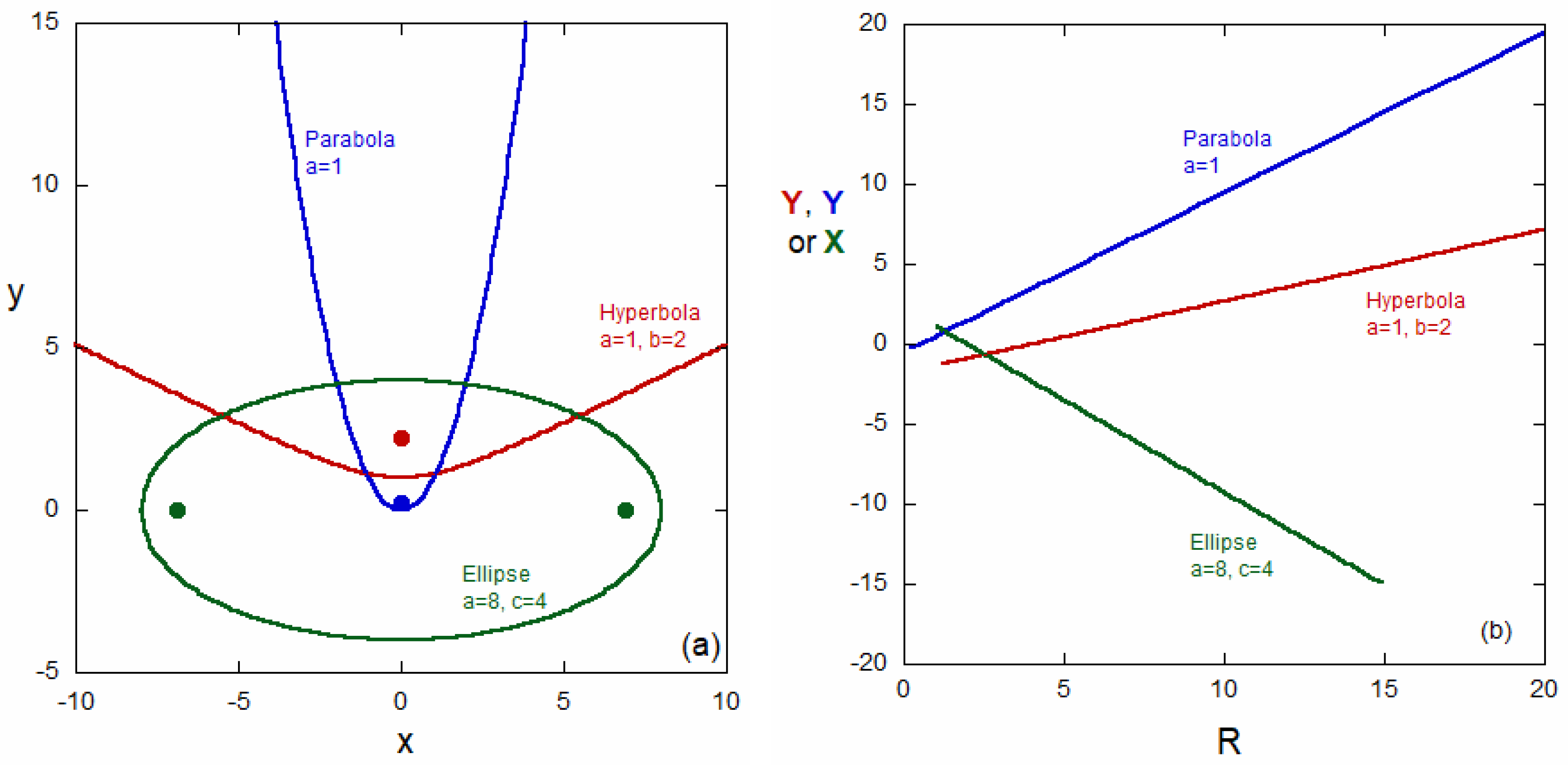
Detailed geometrical analysis of hyperbolic paths is warranted for two additional reasons. First, in standard physics treatments, the energy, momentum and velocity of a particle in a central force field are presented solely as a function of radial distance to the focus (e.g., [5]). Yet, elliptical, parabolic, or hyperbolic paths are typically described in terms of Cartesian coordinates that are not centered on the focus (Figure 1a). The present paper shows that numerous advantages and simplifications arise when the geometry of particle paths are presented in a different Cartesian coordinate system (Figure 1b), one that is centered on the occupied focus. Section 3.1 provides the well-known equations for the conventional representation of Figure 1a whereas Section 3.2 and Section 3.4 derive the equations for the transformed coordinate system shown in Figure 1b.

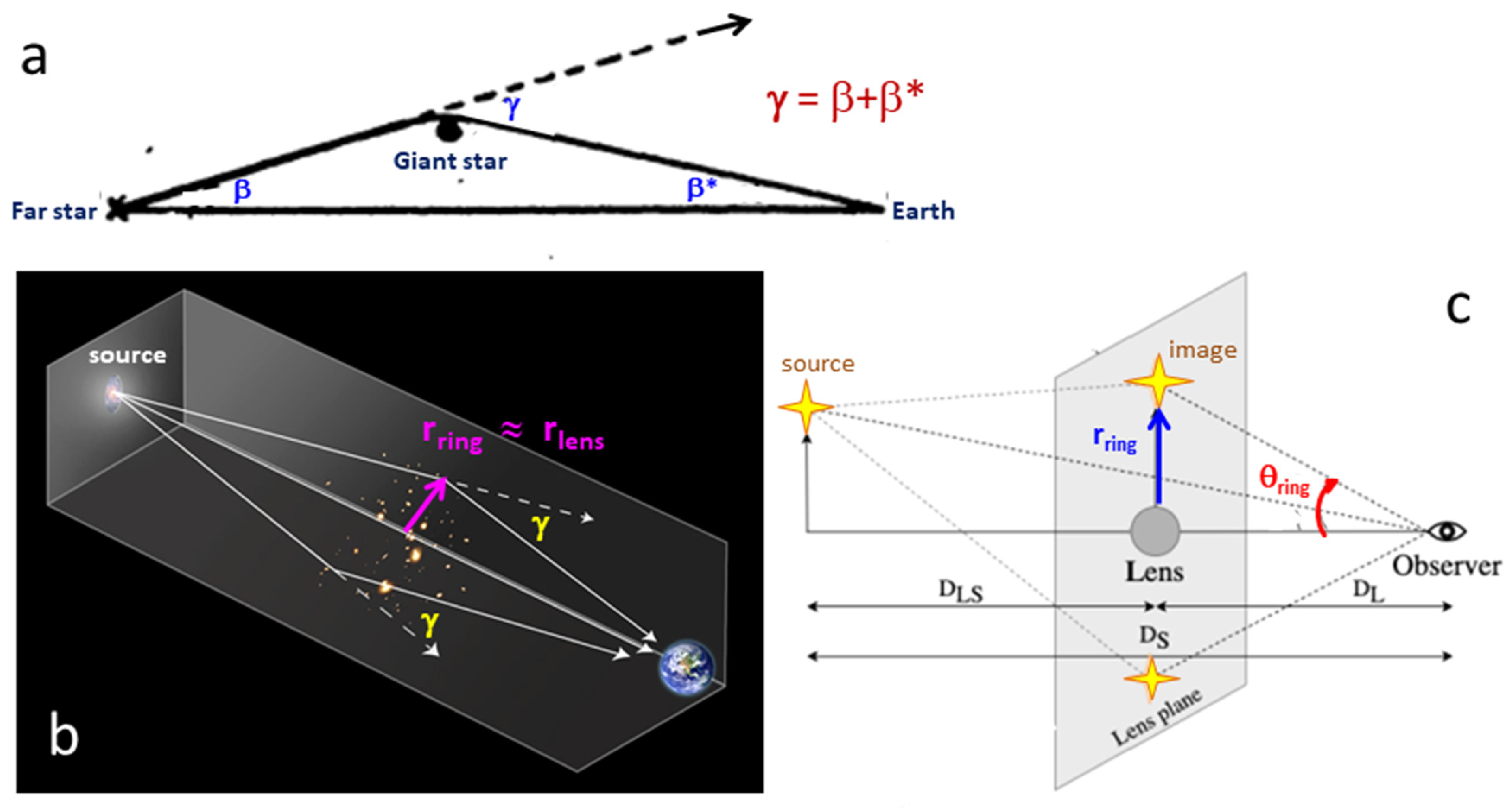
Second, hyperbolic trajectories pertain to the bending of light, a topic of historical and modern importance to physics and astrophysics. Classical geometric constructions [9,10,11] are based on the asymptotes, as is also the case for Einstein’s general relativity construction [12]. Background Section 2.1 and Section 2.2 respectively describe historic and modern constructions, and their relevance to current research in strong gravitational lensing. Specifically, images of galaxies and quasars from space telescopes (the Hubble and Gaia missions) are analyzed to find examples of a galaxy (or quasar) bending the light from a more distant source, commonly a quasar (e.g., [13,14,15,16,17,18,19,20]). Obviously, finite distances are involved, and so asymptotic limits need not apply. Section 2.3 provides details and explains why an algebraic geometric description of the entire hyperbolic path, which involves several angles, is warranted.

1.1. Purpose of the Paper

Approximations to hyperbolic trajectories remain in use because the entire path is not always observed. Reliance on approximations has blurred the mathematical distinctions between several different angles and quantities that are intrinsic to hyperbolic paths. To precisely define and quantify the special angles related to the hyperbola, the present paper utilizes algebraic geometry and provides visualizations of these angles. The case of collinearity involving the focus and two points that lie on opposite limbs of the hyperbola is also investigated here because this configuration pertains to analysis of images of galaxies (or quasars) for strong gravitational lensing (e.g., [13,14,15,16,17,18,19,20]). With these purposes in mind, the paper places special emphasis on the hyperbolic path of a particle or light ray that intersects the position of an observer.

The present paper considers central (Newtonian) forces and finite distances in Euclidean space. New depictions for hyperbolae, based on focus-centered coordinate systems, should prove useful for physical analysis of particle trajectories in several situations (e.g., comets, Rutherford scattering [3,4,5,6,7,8]). Improved classical descriptions of hyperbolic paths should provide a useful reference point for relativistic analysis of galactic lensing.

1.2. Organization of the Paper

Section 2 provides the background. Section 3 provides a coordinate transformation that allows the hyperbola and all other conic curves to be recast as a linear relationship between radius R and either coordinate Y or X, as illustrated in Figure 1b. This compact relationship facilitates the quantification of important angles that are relevant to classical analysis of trajectories. Except for the few with an approximately equals sign, all formulae in Section 3 are exact and general, and many are new. We highlight the importance of the impact angle, which is defined here and associated with the conserved quantity of angular momentum, but has not been utilized in prior analyses of bending. Section 4 discusses our results and points to future work. Section 5 concludes.

2. Background: Physics and the Geometry of the Bending of Light

2.1. Classical Treatments of the Hyperbolic Trajectories of Light

Gravitational bending of light as a possibility was first mentioned by Newton [21] in 1704 in the prescient Queries 1, 4 and 5 of his Optics. Query 1 asks, “Do not bodies act upon light at a distance, and by their action bend its rays, and is not this action strongest at the least distance?” Subsequent classical predictions of gravitational forces bending light rays were made by others, for example by Cavendish circa 1784, as discussed by Lotze and Simionato [9], and by von Soldner in 1801, as translated by Jaki [10]. Early studies treat light as a particle. Lotze and Simionato [9] thoroughly discuss these early studies and include printed material from Cavendish that was not previously discussed.

Due to the difficulty of calculating the deflection angle of a hyperbolic trajectory at a random position, these classical analyses and the 1925 paper by Chwolson [11] are limited to points on the asymptotes. Moreover, classical analyses are based on the law of deviation because different hyperbolic paths are described by different asymptotes. Yet, all parts of hyperbolic paths are valid descriptions of a possible gravitational trajectory.

The law of deviation describes the perturbed light ray solely in terms of departure from its straight initial path by some angle (Figure 2a), currently denoted as the angle of deflection. Although the path is depicted as a tiny arc or circle near the massive body (e.g., Figure 2a), portraying the distal part of the trajectories is the essence of previous classical analyses. The distal parts of a hyperbolic path are nearly straight lines that are coincident with its asymptotes, as summarized in Chwolson’s [11] schematic (Figure 2a).

Classical analysis of gravitational bending of light (e.g., [9,23]) provides the angle of deflection (δ) as:

$$\delta \cong {\displaystyle \frac{2GM }{b{V}_{\infty }^2}}= {\displaystyle \frac{2GM }{b{c}^2}},$$

(1)

where G is Newton’s gravitational constant, M is the mass of the massive central object, b is the semi-minor axis of the particular hyperbola (Figure 3), and $V_{\infty }$ is the “hyperbolic excess velocity” of the travelling mass at infinite distance (see Appendix A). Chwolson [11] used γ for the angle of deflection, as shown in Figure 2a,b, and did not use the small angle approximation. We use δ as in Figure 3 because this symbol suggests the small angles of interest to modern astrophysics. Equation (1) is commonly presented with equals signs, but as shown in Section 3, it is a small angle approximation.

It is well known that for hyperbolic trajectories, conservation laws require that the semi-major axis a equals GM/$V_{\infty }^2$. Figure 3 shows a, b and δ in the conventional x,y coordinate system. By equating the speed $V_{\infty }$ at infinite distance to c, the classical approach evades addressing the implied acceleration of light corpuscles to speeds > c near the periapsis. Equation (1) requires extremely large distances, as the hyperbola and its asymptotes only truly coincide at infinity.

Importantly:

Remark 1.1.

The law of deviation in Euclidean space is identical to the triangle sum theorem, as shown in Figure 2a.

Remark 1.2.

Because the triangle sum theorem is true regardless of the force causing bending in Euclidean geometry, the angles and labels used by Chwolson [11] (Figure 2a) are not used in the present paper. Instead, we use δ for the deflection angle, as in more recent work, and define additional relevant angles in Section 3.1.

Definition 1.3.

The deflection angle δ, equal to π − α, is the angular change in direction of a mass (or ray) following an infinitely long path. This angle is a constant for any particular hyperbola and is defined by its asymptotes (Figure 3).

2.2. Use of the Law of Deviation in Relativistic Treatments of Light Bending

Einstein [12] in 1936 stated “It follows from the law of deviation that an observer… will perceive a luminous circle of angular radius…”. As in the classical approaches, he depicted paths as asymptotes of some hyperbola. An additional assumption is that the deflection angle is small. For derivations see, e.g., [24,25,26]. The final result for the relativistic deflection angle is:

$$\delta ={\displaystyle \frac{4GM }{b{c}^2}}.$$

(2)

Einstein [12] did not provide a figure. His text suggests that he had Chwolson’s [11] deflection angle in mind, which is γ in Figure 2a or angle δ in Figure 3.

A simple, heuristic explanation for the value for δ provided by Equation (2) being double the classical result of Equation (1) is that light experiences equal amounts of space and time curvature, and thus light bends twice as much as in Newtonian theory.

2.3. Relationship of Formulae Depicting Strong Gravitational Lensing to Euclidean Constructions

Recent astronomical searches for evidence of gravitational bending of light by galaxies incorporate Equation (2) in a geometric construction similar to Figure 2b,c (e.g., [20,27,28]). The ideal case (formation of a perfect ring image while a direct image of the source is not observed) is described by:

$${\Theta }_{ring}=\sqrt{{\displaystyle \frac{4G{M}_{lens}}{c^2}}{\displaystyle \frac{D_{source-lens}}{D_{source}{D}_{lens} }}},$$

(3)

where Θ_ring is the measured angular radius associated with light from the source (often a quasi-stellar object); M_lens is mass of the foreground lensing galaxy (which may be a quasar); D_source and D_lens are the angular diameter distances from the observer to the source or lens [15,16,22,28]. The construction is Euclidean, as shown in Figure 2c and noted by [22]. However, the angular diameter distance between the source and lens (D_source-lens) need not equal the difference D_source − D_lens in the current cosmological models used to extract distances from redshift measurements.

Actually, Equation (3) shows that Θ_ring is not an angle associated with the path taken by light but rather is a quantity based on a ratio of distances. Portrayal of Θ_ring as an angle stems from astronomical measurements reporting angular sizes of objects and because conversion of angular size to length requires knowing the distance to the object. Some formulations provide the radius or diameter of the ring instead of Θ_ring (e.g., [13]), because ring diameter links to the mass (e.g., [22]). Analysis of images may also account for elliptical ring shape and/or velocity dispersion (e.g., [13,15]), but these formulae likewise contain a simple numerical factor that embodies relativistic over classical effects (Equation (2) vs. Equation (1)), which is combined with a geometrical ratio of distances. Notably, the combination of distances in Equation (3) results from assuming both that the source and observer are located on asymptotes, and that angles are very small (e.g., [27]). To emphasize small sizes of the angles involved, we point out that the radius of the ring is generally smaller than the radius of the lensing galaxy [14,15]. For very few cases, the ring is larger, but remains similar to galaxy radius [19,20].

Because the asymptotes are invoked through considering the angle of deflection, immense distances that approach infinity are implicit. To address finite distances, the curved portion of the hyperbolic trajectory needs quantification. The present paper explores the Newtonian analogue of gravitational lensing.

3. Coordinate Transform and Linearization in Y, R Coordinates

3.1. Standard Mathematical Description of the Symmetrical Presentation

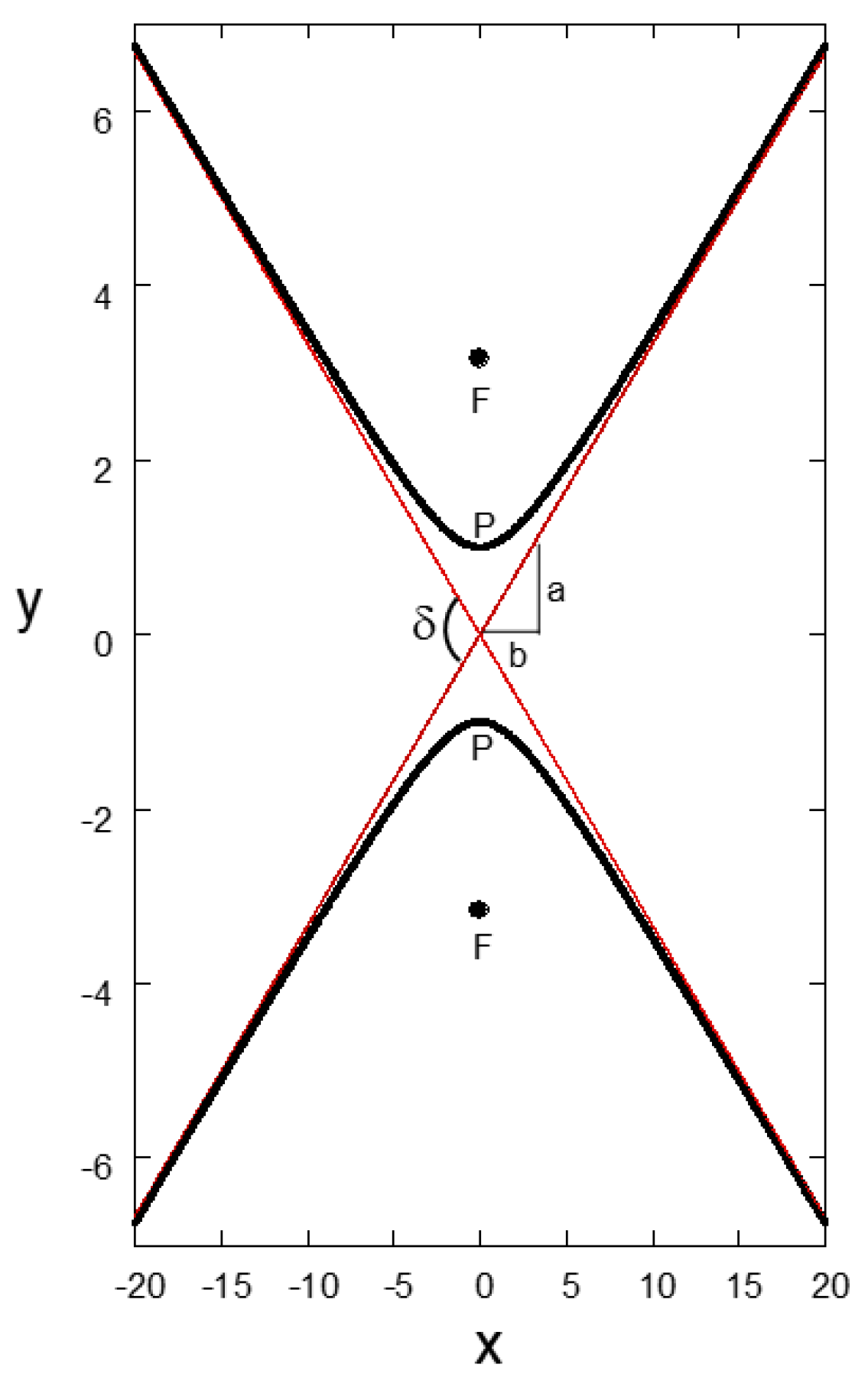
The standard mathematical depiction of an “upright” hyperbola uses an x, y coordinate system whose origin lies at the intersection of the two asymptotes (Figure 3):

$${\displaystyle \frac{y^2}{a^2}}-{\displaystyle \frac{x^2}{b^2}}=1.$$

(4)

Constants a and b are respectively the semi-major and semi-minor axes of the particular hyperbolic curve, and together define the location of its focus f above that curve, which lies at x = 0 with a y-coordinate of:

$$f=\sqrt{a^2+b^2} =ae,$$

(5)

where e is the eccentricity of the hyperbola, equal to $\sqrt{1+b^2/a^2}$.

3.2. Basic Relationships in the Transformed Coordinate System

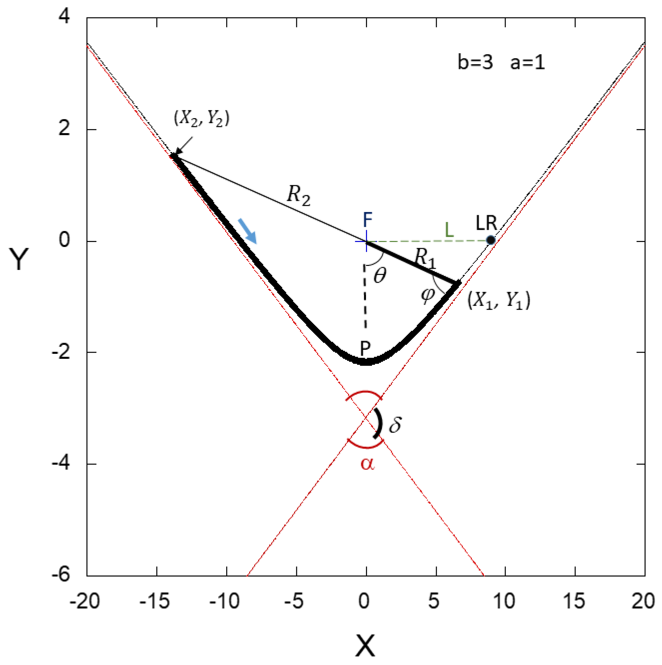
Based on Kepler’s insight, the hyperbolic trajectory is recast into an X, Y coordinate system that is centered on the occupied focus (Figure 4). The analogue of Equation (4), depicted in this new coordinate system (Figure 4), is derived using the transformation:

$$y=Y+f \mathrm{a}\mathrm{n}\mathrm{d} x=X.$$

(6)

This provides:

$${\displaystyle \frac{{(Y+f)}^2}{a^2}}-{\displaystyle \frac{X^2}{b^2}}=1.$$

(7)

When expressed in polar coordinates (e.g., Symon [5], wherein the negative branch in his Figure 3.39 and his Equation 3.248 are germane), the hyperbola is likewise centered on the focus:

$$R={\displaystyle \frac{{a(e}^2-1)}{1+e\mathrm{c}\mathrm{o}\mathrm{s}\left(\theta \right)}},$$

(8)

where R is the radial distance between an arbitrary point on the hyperbola and the focus with length$\sqrt{X^2+Y^2}$, and θ is the position angle of the moving mass relative to the periapsis (Figure 4).

The X, Y and R, θ representations have several advantages over the standard x,y representation for dynamic analysis:

Remark 3.1.

Coordinates X and Y and radial distance R of a point on the hyperbola are all anchored to a common, physically meaningful origin (the occupied focus).

Remark 3.2.

The slope of the radial line connecting the focus with any point on the hyperbola is given by the compact ratio, Y/X.

Remark 3.3.

As shown below, Y is a linear function of the radial distance R. The simplicity of this variable combination greatly facilitates derivations of special angles, and quantifies these angles without relying on the triangle sum theorem or the asymptotic approximation, as done in previous efforts (Figure 2a).

Remark 3.4.

Note that position angle θ has a clear geometric definition. This angle is not the same as Θ_ring of Equation (3), which is the angular diameter shown in Figure 2c.

Remark 3.5.

The velocity V of a particle at any point on a hyperbolic path is easily derived in the focus-centered system using conservation laws (Appendix A).

3.3. Angles of Hyperbolic Paths and Their Connection with Collinear Arrangements

Angle φ between the instantaneous particle direction and the radius (Figure 4) is here termed the impact angle. This angle is of paramount importance because the angular momentum (₤), defined as:

$$₤=mVR \mathrm{s}\mathrm{i}\mathrm{n}\left(\phi \right)$$

(9)

is constant along the entire hyperbolic trajectory.

The impact angle depends on the specific position of the observer on the hyperbola. Many hyperbolic paths are possible, since sources emit light (or particles) radially. Hence, quantifying φ for any given hyperbolic trajectory is crucial to understanding the dynamics of light being bent by gravity at finite distances.

This need is underscored by considering the assumption in classical analysis that the light begins its traverse at some place on one asymptote, which requires distances approaching infinity. Hence, Figure 4 indicates a starting point nearly on an asymptote. This realistic configuration approximates the idealized geometry, where the observer is on (or nearly on) the other asymptote (e.g., Figure 2), as considered in classical and relativistic analyses of the gravitational bending of light (see Section 2; [22,27]).

Remark 3.6.

The impact angle φ varies continuously along a hyperbolic path, and clearly is not the same as the deflection angle δ which is a constant for any given hyperbola (Figure 4). The impact angle is quantified in Section 3.8.

Figure 4 includes the Euclidean construct analogous to Equation (3) where the source (position 2), and a foreground, lensing galaxy or quasar (defining the focus), and the receiving telescope (at position 1) form a straight line of finite length. Figure 4 shows a section of a hyperbolic path (indicated by the heavy line) from the source to the observer. The angle of the bent ray extracted from the image of the lensing galaxy is the angle φ between the line segment 2-F-1 and the light path ending at the observer’s telescope.

Remark 3.7.

Presuming that the ray begins and ends at great distance from the focus, as in historical efforts, is incompatible with those points being collinear with the focus.

3.4. Special Points and Key Formulae in the New (X, Y) Coordinate System

From Equation (7), the periapsis P, which is the point closest to the focus, resides at (0, a − f), while the semi-latus rectum points occupy (±b²/a, 0); see Figure 4. The asymptotes of the upright hyperbola are the lines:

$$Y=\pm {\displaystyle \frac{a}{b}}X-f \mathrm{for} \mathrm{the} \mathrm{asymptotes}.$$

(10)

We emphasize the qualifier on the RHS because most of our other equations depict the actual path.

Importantly, if the definition of R is introduced into the focus-centered hyperbolic curve (Equation (7)), algebraic manipulations involving the quadratic formula can be used to recast Equation (7) into the variable pair (R, Y) instead of (X, Y). The key result for the hyperbola can thus be expressed as:

$$Y={\displaystyle \frac{-b^2+aR}{f}}.$$

(11)

An equivalent linear result between these variables can also be obtained by cross-multiplying Equation (8) and noting that Y = −R cos(θ) for the upright hyperbola of Figure 4. Considering polar representations for all three types of conic sections (e.g., [5]) leads to the following proposition, which is illustrated in Figure 1b:

Proposition 3.8.

All conic curves can be translated to an origin coincident with the focus, and then rotated about the focus to an orientation symmetric about the Y-axis where the following linear relation holds:

$$R=eY+L,$$

(12)

where e is the eccentricity defined by the major and minor axes, and L is the length of the semi-latus rectum for the hyperbola, parabola or ellipse.

Rotation of the orientation in Figure 4 by 180° provides the same equation with a change in sign of the eY term, whereas a clockwise rotation by 90° provides the same relation if Y is replaced by X.

3.5. Important Ratios in the Transformed System

Equation (11), graphically illustrated in Figure 1b, is important for several reasons. First, the distance R between the travelling mass and the focus is the key length variable in orbital dynamics. Second, in this new, focus-centered coordinate system, coordinate Y depends linearly on the distance R. This latter condition greatly simplifies deducing the properties of the hyperbola and allows many of them to be compactly expressed as functions of R alone. For example, the slope of a hyperbola at any point on the curve depends only on its X coordinate:

$${\displaystyle \frac{dY}{dX}}={\displaystyle \frac{aX}{b\sqrt{X^2+ b^2 }}},$$

(13)

which equals 0 at the periapsis, and ±a/f at the semi-latus rectum points. Similarly, the Y/X ratio of any such point is:

$${\displaystyle \frac{Y}{X}}=\pm {\displaystyle \frac{aR-b^2}{b\sqrt{{\left(R+a\right)}^2-f^2}}}.$$

(14)

3.6. Vertex Angle Between Asymptotes and the Total Deflection Angle

Several different angles are of interest in the dynamic analysis of hyperbolic paths (Figure 2, Figure 3 and Figure 4). Two angles were considered previously. One is the angle α between the asymptotes; another is the total deflection angle δ experienced by a mass on a path beginning and ending at infinite distances from the focus.

The value of angle α between the asymptotes is easily reasoned using Figure 4, given that the slope of an asymptote is simply ±a/b (Equation (10)). If a vertical line is constructed through the asymptote intersection, angle α is precisely bisected, and the tangent of that half angle is clearly b/a. Similarly, construction of a horizontal line through the asymptote intersection bisects the deflection angle δ and the tangent of that half angle is clearly a/b; see Figure 4. The exact relations are thus:

$$\mathrm{t}\mathrm{a}\mathrm{n}\left[\alpha /2\right]={\displaystyle \frac{b}{a}} \mathrm{a}\mathrm{n}\mathrm{d} \mathrm{t}\mathrm{a}\mathrm{n}\left[\delta /2\right]={\displaystyle \frac{a}{b}}$$

(15)

Remark 3.9.

Considering that the asymptotes are germane to gravitational bending implicitly assumes that R is extremely large. Yet, a and b can take on any values.

If δ is small, the near equivalence of the tangent and radian measures can be used to simplify Equation (15) (right-hand side, RHS), providing the approximation:

$$\delta \cong {\displaystyle \frac{2a}{b}} \mathrm{f}\mathrm{o}\mathrm{r} b\gg a, i.e., e\gg 1$$

(16)

3.7. Deflection Angle for a Finite Path

The partial deflection angle δ_p of a mass that moves between any two points A and B on the hyperbola is easily calculated using Equation (13):

$${\delta }_p=\left|\left|{\mathrm{a}\mathrm{r}\mathrm{c}\mathrm{t}\mathrm{a}\mathrm{n}\left({\displaystyle \frac{dY}{dX}}\right)}_B\right|\pm \left|{\mathrm{a}\mathrm{r}\mathrm{c}\mathrm{t}\mathrm{a}\mathrm{n}\left({\displaystyle \frac{dY}{dX}}\right)}_A\right|\right|.$$

(17)

The positive sign is used if points A and B are on opposite limbs of the hyperbola, whereas the terms are subtracted if A and B lie on the same side. If distances are large, dY/dX approaches ±a/b (Equation (13)), in which case Equation (17) is consistent with Equation (16).

3.8. Geometric Quantification of the Impact Angle

Angle φ is the instantaneous angle of approach of the moving particle to an arbitrary point occupied by an observer, measured relative to the radial line to the focus (Figure 4). The flight path angle (not labeled) is the complement of this angle, i.e., the quantity π/2 − φ, which is the instantaneous path direction relative to the perpendicular to R.

The impact angle can be conveniently derived from the physical requirement of angular momentum conservation along the trajectory (Appendix A). The exact result, here expressed in geometric terms, is:

$$\phi =\mathrm{a}\mathrm{r}\mathrm{c}\mathrm{s}\mathrm{i}\mathrm{n}\left[{\displaystyle \frac{b}{\sqrt{R(R+2a)}}}\right].$$

(18)

The impact angle at the observer’s location is obtained by replacing R by R₁.

Our new, compact results provide another convenient, yet exact, classical evaluation of φ. At any point on the hyperbolic curve, angle φ is related to the slope of the radial line to the focus, and to the derivative dY/dX of the hyperbola at that point (Figure 4). The angle for the first of these contributions is arctan [Y/X]. The second angle is arctan [dY/dX]. These two contributions provide:

$$\phi =\left|\arctan \left[{\displaystyle \frac{Y}{x}}\right]-\mathrm{a}\mathrm{r}\mathrm{c}\mathrm{t}\mathrm{a}\mathrm{n}\left[{\displaystyle \frac{dY}{dX}}\right]\right|$$

(19)

Here, angle φ is treated as a positive quantity. A useful result is obtained at the latus rectum point, where Y = 0 and X = b²/a:

$${\phi }_{LR}=\mathrm{a}\mathrm{r}\mathrm{c}\mathrm{t}\mathrm{a}\mathrm{n}\left[{\displaystyle \frac{a}{f}}\right]=\mathrm{a}\mathrm{r}\mathrm{c}\mathrm{t}\mathrm{a}\mathrm{n}\left[1/e\right]$$

(20)

Interestingly, for the case where b >> a, for which f is approximately b, comparison of Equations (15) and (20) shows that φ at the semi-latus rectum point is very close to δ/2.

3.9. Requirements for a Collinear Configuration

Here we consider two points along the trajectory that are collinear with the focus as in Figure 4, since this is the classical analogue of the configuration illustrated in Figure 2b. These two points are denoted by subscripts 1 and 2 in Figure 4, and lie at respective distances of R₁ and R₂ on opposite limbs of the hyperbolic curve. Consequently, these points lie on a straight line through the focus that is particular to the R₁ and R₂ pair. The relation for similar triangles provides the equation:

$$-{\displaystyle \frac{R_2}{R_1}}={\displaystyle \frac{X_2}{X_1}}={\displaystyle \frac{Y_2}{Y_1}}$$

(21)

Introducing Equation (11) for the upright hyperbola into Equation (21) specifies the ratio of coordinates Y₂ and Y₁:

$${\displaystyle \frac{Y_2}{Y_1}}={\displaystyle \frac{{-b^2+aR}_2}{-b^2+a{R}_1}}=-{\displaystyle \frac{R_2}{R_1}}.$$

(22)

Several important relationships can be deduced from the above equations. Cross multiplying and collecting terms in one way allows R₂ to be expressed as a function of R₁:

$$R_2={\displaystyle \frac{{R_{1}b}^2}{2a{R}_1{-b}^2}}.$$

(23)

This expression shows that collinearity requires that R₁ must exceed its minimum value of b²/2a, which is one half of the radius at the semi-latus rectum point. An alternate way of collecting terms provides another key expression:

$${\displaystyle \frac{R_2}{R_1+R_2}}={\displaystyle \frac{b^2}{2a}}{\displaystyle \frac{1}{R_1}}.$$

(24)

So:

$$\sqrt{{\displaystyle \frac{2a{R}_2}{R_1\left(R_1+R_2\right)}}}={\displaystyle \frac{b}{R_1}} \equiv {\Theta }_c$$

(25)

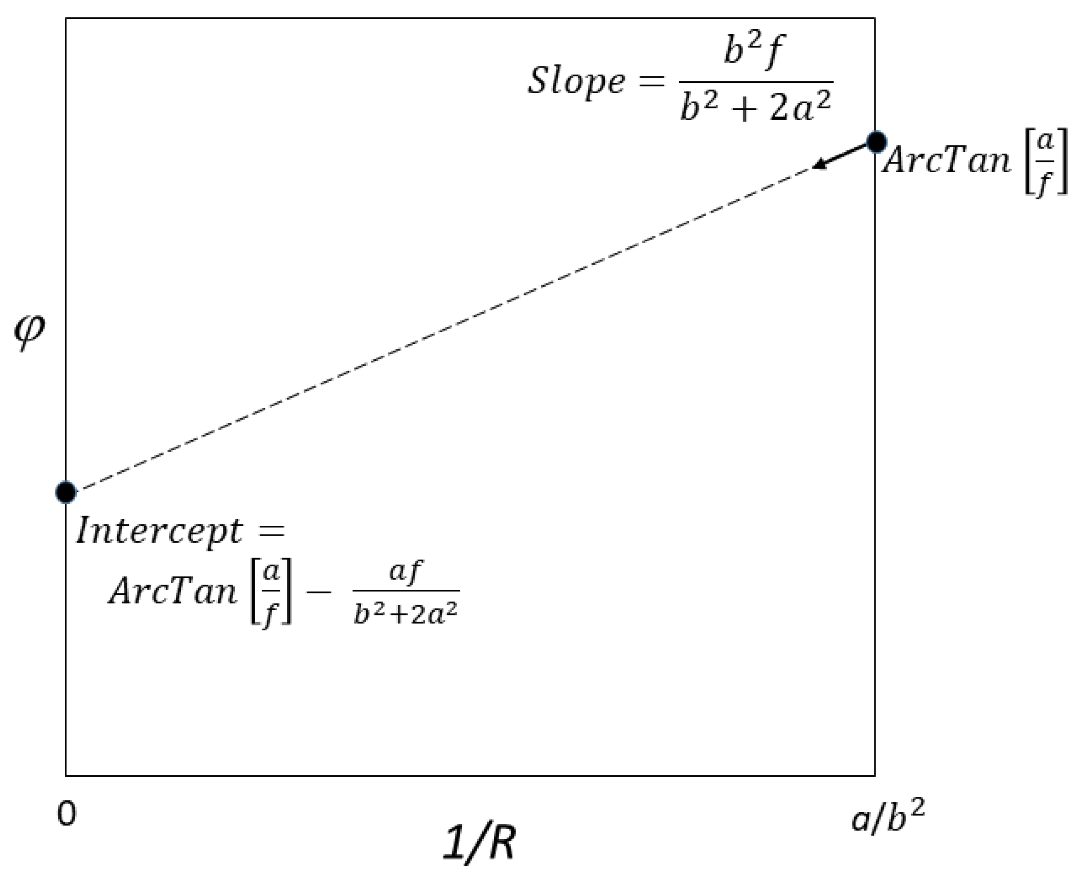
Equation (25) is an exact classical property of a hyperbolic trajectory and describes a ratio that we define as ${\Theta }_c$, given the similarity of its left-hand side to Equation (3). It is therefore important to establish the relation of the parameter combination in Equation (25) to angle φ, which is most easily done by investigating the relationship between φ and 1/R₁.An approximate linear result for this line is derived in Appendix B:

$$\phi \cong \left({\displaystyle \frac{b^2}{b^2+2a^2}}\right){\displaystyle \frac{f}{R_1}}+\mathrm{a}\mathrm{r}\mathrm{c}\mathrm{t}\mathrm{a}\mathrm{n}\left[{\displaystyle \frac{a}{f}}\right]-{\displaystyle \frac{af}{b^2+2a^2}}$$

(26)

Precisely at the latus rectum point, the first and third terms on the right side cancel, returning Equation (20). Importantly, over the very wide range of R₁ allowed by collinearity, Equation (26) is highly accurate, though it is only exact at the latus rectum (Figure 5).

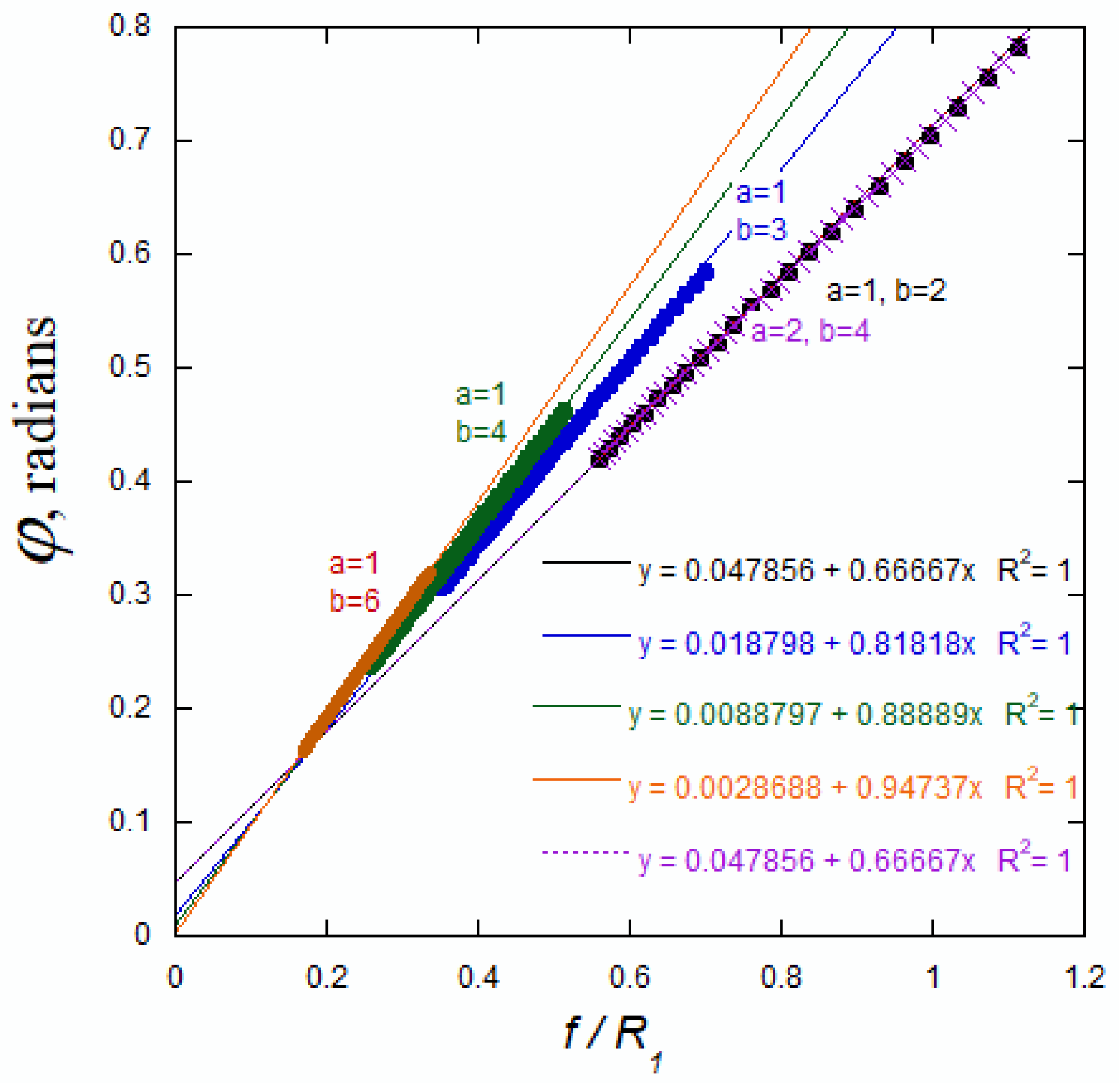
Points allowed by collinearity for several different hyperbolae were exactly calculated at uniform intervals using Equation (18), and are presented in Figure 5. The straight lines in Figure 5 represent Equation (26), and these lines closely match those precisely calculated points. These plotted points span all possible values of R₁ in the lower right quadrant of the various hyperbolae that are allowed by collinearity (see Appendix C); points falling at the lower left of each group represent an observer at the latus rectum point, for which case R₁ and R₂ are equal. Multiplying a and b by a common factor results in coincident points, as illustrated by the case on the far right of Figure 5 (burgundy and black colors). Thus, Equation (26) is remarkably accurate over a wide range.

Figure 5 demonstrates the high degree of linearity between φ and f/R₁, as well as the existence of an intercept on the left-hand (φ) axis for the points allowed by the collinearity requirement. Furthermore, Figure 5 and Equation (26) emphasize that the limiting y-intercept of φ → 0 is approached only when b >> a, because the right two terms of Equation (26) vanish as b → ∞.

3.10. Comparison of Impact Angle φ, Angle δ/2 and Ratio Θ_c Under the Condition of Collinearity

Here we consider two points along the trajectory that are collinear with the focus, whose respective radial distances from the focus differ by a factor of n; that is, R₂/R₁ = n. Given these dual conditions, the aforementioned relationships allow angle φ, angle δ/2 and the ratio Θ_c defined in Equation (25) to all be expressed as functions of the ratio a/b of any hyperbola. Three exact relationships result. First, the half-angle of deflection, defined in Figure 3 and Figure 4, is simply:

$${\displaystyle \frac{\delta }{2}}=\mathrm{a}\mathrm{r}\mathrm{c}\mathrm{t}\mathrm{a}\mathrm{n}\left[{\displaystyle \frac{a}{b}}\right]$$

(27)

The impact angle φ shown in Figure 4 is:

$$\phi =\mathrm{a}\mathrm{r}\mathrm{c}\mathrm{s}\mathrm{i}\mathrm{n}\left[2n/\sqrt{{{ \left(n+1\right)}^2\left(b/a\right)}^2+4n^2+4n} \right]$$

(28)

and the ratio defined in Equation (25) is:

$${\Theta }_c=\left({\displaystyle \frac{2n}{n+1}} \right)\left({\displaystyle \frac{a}{b}}\right)$$

(29)

These relationships all reduce to the equations presented earlier in this report for the condition at the latus rectum point, where n = 1. Also, for the condition where a → 0, all of these quantities are equal to zero. Finally, the impact angle φ and the ratio Θ_c converge when b >> a:

$$\phi \cong {\mathsf{\Theta }}_c for b\gg a$$

(30)

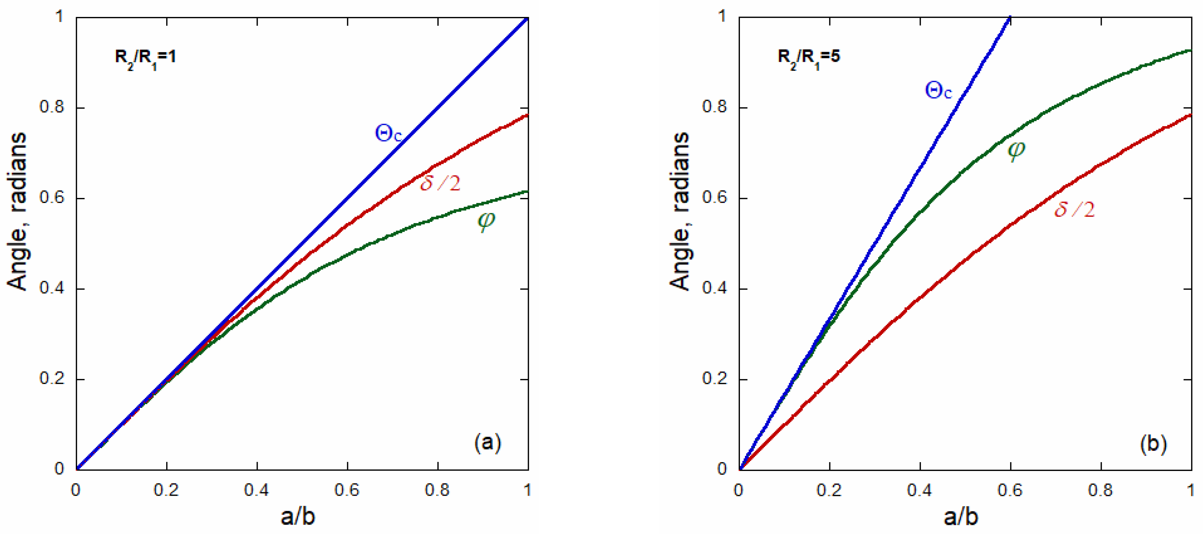
Figure 6 shows the relationship between all three quantities for two cases, one for the latus rectum condition where n = 1, and the other for the condition n = 5.

Note that all three quantities are mathematically different, but they can have similar values under specific conditions.

4. Discussion

The present paper investigates hyperbolic trajectories that arise under Newtonian gravitational and Coulombic forces in Euclidean space, which are of interest historically and to certain modern problems (Section 1 and Section 2). All equations in Section 3 and the Appendix A, Appendix B and Appendix C were cross-checked analytically and also by using spreadsheet computations.

Although our equations describe any hyperbolic path, we chose to focus on one application of great current and historical interest in astronomy: the gravitational bending of light. Previous dynamical formulae regarding light are based on asymptotic behavior, but the limitations of this approximation were scarcely investigated. Although one key parameter of the hyperbola (a) can be related to gravitation without restrictions on b, the angle of bending is indeterminate. To better explore where bending mostly occurs, i.e., near the periapsis, the main body of this report is concerned with quantifying the actual hyperbolic path in Euclidean space.

The objective of quantifying the actual hyperbolic path is furthered by our coordinate transform that anchors all variables to the occupied focus (Section 3). This transform allows either the Y or the X coordinates of all conic sections to be expressed as simple linear expressions involving the radial distance R (Figure 1b), which is key because R is the length parameter of greatest importance in the dynamic analysis of particle motions. This simplification allowed us to quantitatively establish the condition where points on the opposite hyperbolic limbs are collinear with the focus, which configuration is important to gravitational lensing problems. These equations also allowed us to quantify the impact angle φ (Section 3.8) in geometric terms, and to show that it exactly describes bending around the focus (Figure 4). Previous classical efforts instead considered the deflection angle δ between the two asymptotes (Section 2), which does not portray an observable path, but rather describes approximate behavior at great distance (Section 3.6 and Section 3.7).

Our linear equations provide convenient aids in solving geometric problems such as the angles associated with these paths, and permit the errors associated with common approximations to be quantified. Section 4.1 and Section 4.2 provide examples. Our equations also greatly simplify analyses of the dynamic conditions of a moving mass in trajectories and orbits, which is accomplished by invoking conservation of momentum and energy in comparisons of conditions at the periapsis and other special positions (Appendix A).

4.1. Comparison with Previous Classical Results for the Gravitational Bending of Light

Comparing the classical result for the bending of light (Equation (1)) to our exact geometrical result (Equation (15)) and also to its small angle limit (Equation (16)) reveals that Equation (1) is not generally true. Equation (1) is commonly presented only with equal signs; instead, it is a useful approximation only when b >> a, i.e., for flat hyperbolae with large eccentricity. Large eccentricity is compatible with the source (point 2) lying on the left asymptote (of Figure 4) at some great distance, approaching infinity, as well as with the observer (point 1) lying on the right asymptote also at some great distance, approaching infinity. However, if points 1 and 2 lie at great distances along the hyperbola, then these points cannot be collinear with the focus, nor can these three points be even nearly collinear. The visual presentation (Figure 4) shows that points 1 and 2 at finite distances lie off the asymptotes.

Chwolson’s sketch (Figure 2a), where the large mass substantially redirects the small mass (or light ray), recognizes that the source, focus, and observer are not collinear when the asymptotes define the path. Equation (1) is indeed correct for Chwolson’s geometry, but it is not exact. Equation (1) has an exact counterpart in Equation (27), but applying this requires independent knowledge of b. The impact angle provides more information, describes the light seen by the observer, and is not restricted to points that lie on the asymptotes.

4.2. Galactic Lensing Conditions

Images of galaxies which include regions of light with greater redshifts than the main object have been assessed as candidates for strong gravitational lensing using Equation (3), or modifications thereof, and with distances modified to address the cosmology model denoted ΛCDM (e.g., [20,22]). The strong lens formulation is based on asymptotic behavior and small angles (e.g., [22,28]). The source, the lens, and the observer are presumed collinear or nearly so. Hence, the problems discussed in Section 4.1 arise.

Specifically, meeting both criteria of collinearity and asymptotic locations implies that a/b → 0, which is equivalent to b → ∞ for a large mass associated with galaxies. In this case, R₂ and R₁ both → ∞. Images, however, represent objects at finite distances.

4.3. Future Work

Conic sections describe numerous cases of particles subject to an inverse square force. Hence, many applications may benefit from the simplifications provided here.

Regarding the bending of light, although relativistic calculations are beyond the scope of the present paper, the exact Euclidean analysis provided here points to possible future directions for ascertaining candidacy of galaxy images for strong gravitational lensing. As discussed above, the source, focus, and observer (impact point) are generally not collinear. In a Euclidean geometry, the angle of impact needs to be used, as this is what can be observed. Triangular configurations (e.g., small deviations from collinearity) need to be further investigated.

We emphasize that we are not contesting the equations for bending of light, whether classical or relativistic, but are pointing out that formulations used to evaluate strong lensing by galaxies are based on asymptotic delivery of light from nearly infinite distances. But because finite distances are involved, bending of light near the foreground galaxy (or quasar) needs to be quantified, rather than being approximated by asymptotic behavior. The relevant quantity is not the angle of deflection, but the angle of impact, which embodies conservation laws, is what can be measured, and is quantified in geometric terms here.

5. Conclusions

Using the law of deviation (triangle sum theorem) in historical formulae for the bending of light by gravity and in relativistic adaptations is necessitated by the lack of a geometric formula for the impact angle, which varies along the path. This paper uses a coordinate transform that is motivated by the work of Kepler, as it centers the coordinate system on the occupied focus of the conic curve, providing X = 0 and Y = 0 at the focus. This simple transformation allows any conic section to be recast into the compact linear form, R = eY +L, where e is the standard eccentricity and L is the length of the semi-latus rectum. The simplicity of this form facilitated our derivations of relationships for the hyperbola. Our relationships should have wide applicability.

The present paper explores the Newtonian analogue of gravitational bending. Our quantification of the curved portion of the hyperbolic trajectory improves upon historical and modern studies of light bending. Exact equations that we believe are new and significant include Equation numbers (11) to (14), (18), (25), (28) and (29). Our Euclidean analysis has shown:

• Collinearity of source, lensing object, and observer is only possible at finite distances.
• Asymptotes do not describe the observable parts of hyperbolic paths.
• Formulae for deflection angles are not exact descriptions of light bending (or particle paths), but instead limit bending to small angles while assuming infinite distances.
• The impact angle defined here constrains the actual hyperbolic path, and describes the light that the observer receives.