Machine Learning-Based Imputation for Breast Cancer Prediction: Evaluating Performance Under Complex Missing Data Mechanisms

Abstract

Missing data remain a major challenge in breast cancer research because they can introduce bias, reduce statistical efficiency, and compromise the performance of predictive models. Although numerous imputation techniques have been proposed, their comparative performance under different missing-data mechanisms and their impact on downstream classification remain inadequately understood. This study systematically compared statistical and machine learning-based imputation methods using two publicly available breast cancer datasets representing complementary clinical settings. The methods were evaluated under simulated Missing Completely at Random (MCAR), Missing at Random (MAR), and Missing Not at Random (MNAR) mechanisms using both reconstruction accuracy and downstream classification performance. The results showed that no single imputation method consistently achieved the best performance across both datasets. Regularized regression and machine learning-based methods generally outperformed conventional statistical approaches, although the optimal method depended on the characteristics of the dataset. Furthermore, the best-performing imputation methods preserved downstream classification performance despite the introduction of missing data, demonstrating that reconstruction accuracy alone is insufficient for selecting imputation strategies intended for predictive modelling. Overall, the findings highlight the importance of considering dataset characteristics, missing-data mechanisms, and the intended analytical objective when selecting imputation methods. The proposed evaluation framework provides a robust approach for assessing missing-data handling strategies in breast cancer prediction studies and other biomedical machine learning applications.

1. Introduction

Breast cancer remains one of the most prevalent cancers worldwide and a leading cause of cancer-related mortality among women. According to the World Health Organization, breast cancer accounts for a substantial proportion of new cancer cases globally (2.3 million women diagnosed in 2022, resulting in 670,000 deaths), emphasizing the need for improved diagnostic methods and predictive modelling techniques [1]. Advances in medical technologies, including genomic sequencing, radiomics, and electronic health records, have resulted in the generation of large volumes of biomedical data that can be used to support early detection and personalized treatment strategies. Many breast cancer diagnostic studies now rely on datasets, such as gene expression profiles, imaging features, and clinical variables, where thousands of predictors may be measured for each patient [2]. While these datasets provide valuable insights for disease prediction, they also introduce several analytical challenges, one of the most important being the presence of missing data.

Missing values are a common occurrence in breast cancer datasets due to various factors such as incomplete clinical records, equipment failure during diagnostic procedures, data entry errors, and patient attrition during clinical studies. In high-throughput technologies such as microarray and RNA-sequencing experiments used to identify breast cancer biomarkers, missing entries may also arise from technical limitations or measurement noise during data acquisition [3]. The presence of missing data complicates statistical analysis and machine learning modelling, as many algorithms require complete datasets for accurate parameter estimation. If missing values are not handled appropriately, they can lead to biased model estimates, reduced statistical power, and unreliable predictive performance [4].

Traditional approaches for handling missing data include deletion methods and simple statistical imputation techniques. For example, complete case analysis removes observations containing missing values before analysis. Although this approach is simple to implement, it often results in significant loss of information and may introduce bias when the missingness is not completely random. Similarly, basic imputation methods such as mean or median substitution fail to capture the complex relationships among variables and may distort the underlying data distribution [5]. Consequently, these conventional approaches are often inadequate for analysing complex biomedical datasets such as those used in breast cancer prediction.

Machine learning techniques have increasingly been adopted to overcome the limitations of traditional imputation approaches [6,7,8]. Unlike simple statistical methods, machine learning-based imputation algorithms are capable of capturing complex nonlinear relationships among variables and leveraging correlations within high-dimensional datasets. Common machine learning imputation techniques include k-Nearest Neighbor (kNN) imputation, Random Forest-based imputation (MissForest), decision tree models, and neural network-based methods. These algorithms estimate missing values by learning patterns from observed data and predicting plausible values for missing entries [9]. Several studies have demonstrated that machine learning imputation approaches often outperform traditional statistical methods in terms of imputation accuracy and predictive model performance in biomedical applications [10].

The problem of missing data becomes even more challenging in breast cancer datasets, especially those derived from genomic studies or clinical settings. Gene expression datasets may contain thousands of features, while the number of patient samples remains relatively small. This “large p, small n” problem increases the difficulty of accurately estimating missing values and may lead to unstable model estimation, multicollinearity, and increased risk of overfitting [11]. Consequently, effective missing data handling techniques are essential for maintaining the reliability and robustness of machine learning models used in breast cancer prediction.

Another critical characteristic of breast cancer datasets is class imbalance, where the number of samples in one class significantly exceeds the number in another. In many diagnostic datasets, benign cases greatly outnumber malignant cases, or non-cancer cases outnumber cancer cases. This imbalance presents a challenge for machine learning models because most algorithms tend to favour the majority class during training, which may reduce the ability of the model to accurately detect cancer cases that are clinically more important [12]. Imputation methods that do not account for class imbalance may further exacerbate this problem by reconstructing missing values based primarily on patterns from the majority class.

In addition to these challenges, the validity of imputation methods depends heavily on the mechanism underlying the missing data process. Rubin’s missing data framework classifies missingness into three mechanisms: Missing Completely at Random (MCAR), Missing At Random (MAR), and Missing Not At Random (MNAR) [5]. Most statistical and machine learning imputation techniques assume that missing data follow the MAR mechanism, where the probability of missingness depends only on observed variables. However, in clinical datasets this assumption may not always hold. When the MAR assumption is violated, imputation models may produce biased estimates that affect the performance of downstream predictive models. As a result, sensitivity analysis is often required to evaluate how imputation results change when the MAR assumption is relaxed [4].

Given the increasing reliance on machine learning techniques for breast cancer diagnosis, it is important to systematically evaluate the effectiveness of imputation algorithms in datasets that are often characterized by class imbalance and complex missingness patterns. Machine learning-based imputation techniques provide promising solutions, but their performance can vary depending on the data structure, level of missingness, and underlying missing data mechanism. Therefore, robust evaluation of these techniques is necessary to identify appropriate strategies for handling missing values in breast cancer diagnostic datasets.

While numerous studies have evaluated individual imputation methods, relatively few have systematically compared traditional statistical approaches, machine learning algorithms, and regularized learning methods under multiple missing-data mechanisms while simultaneously assessing their downstream impact on breast cancer classification performance. Moreover, existing studies often assume the Missing at Random (MAR) mechanism without examining the robustness of imputation algorithms when this assumption is violated. To address these limitations, this study develops a comprehensive simulation framework for evaluating statistical and machine learning-based imputation methods using two publicly available breast cancer datasets representing complementary clinical settings. The framework evaluates imputation performance under MCAR, MAR, and MNAR mechanisms across multiple missingness levels and examines the effect of the imputation methods on downstream breast cancer classification using Logistic Regression, Random Forest, and LightGBM classifiers within a repeated nested cross-validation framework.

This paper focuses on the application of machine learning methods for handling missing data in breast cancer prediction datasets. Specifically, the paper addresses the following objectives:

• To compare the performance of statistical and machine learning-based imputation methods under MCAR, MAR, and MNAR mechanisms across different levels of missingness in breast cancer datasets.
• To evaluate the impact of the imputation methods on downstream breast cancer classification using Logistic Regression, Random Forest, and LightGBM classifiers.

By addressing these objectives, the paper contributes to the development of reliable data preprocessing frameworks that improve the performance and interpretability of machine learning models for breast cancer prediction.

2. Materials and Methods

2.1. Datasets

To evaluate the robustness and generalizability of statistical and machine learning-based imputation methods, two publicly available breast cancer datasets representing complementary clinical settings were used. The Wisconsin Diagnostic Breast Cancer (WDBC) dataset [13] served as a benchmark diagnostic dataset with independent observations, while the Longitudinal Breast Cancer Cohort (LBCC) dataset [14] provided a longitudinal population-based cohort with repeated participant measurements. The use of heterogeneous datasets enabled assessment of imputation performance across different sample sizes, predictor characteristics and data structures.

2.1.1. Wisconsin Diagnostic Breast Cancer Dataset

The WDBC dataset was obtained from the UCI Machine Learning Repository [13]. It comprises 569 breast tissue samples classified as malignant (212) or benign (357), with 30 continuous cytological features extracted from digitized fine-needle aspiration images used as predictors and diagnosis as the binary outcome. The patient identifier was excluded from analysis. Since the dataset contains no missing values, artificial missingness was introduced under controlled experimental conditions.

2.1.2. Longitudinal Breast Cancer Cohort Dataset

The LBCC dataset was derived from the openly available pooled cohort reported by McDonnell et al. [14]. It comprises 5038 women followed longitudinally, including 77 incident breast cancer cases. Predictor variables include demographic, anthropometric, lifestyle and biochemical measurements, while breast cancer status (BC_Case) served as the binary outcome. Because the dataset contains repeated observations for individual participants, all observations from the same participant were retained within the same cross-validation partition to prevent information leakage.

2.1.3. Data Pre-Processing

Data pre-processing was undertaken to establish complete reference datasets prior to artificial missing-data generation. Variables serving only as unique identifiers were excluded from model development, while outcome variables remained fully observed throughout the study. Continuous predictors were retained on their original scales, and categorical predictors were encoded as required by the respective machine learning algorithms. For the WDBC dataset, the patient identifier was removed, leaving 30 predictor variables and one binary outcome. For the LBCC dataset, participant identifiers were retained solely for grouped data partitioning and excluded from model training. To preserve the longitudinal structure and eliminate information leakage, all observations from the same participant were assigned to the same cross-validation fold during model development and evaluation. The characteristics of the datasets are summarized in

Table 1. Characteristics of the study datasets.

Characteristic	WDBC	LBCC
Source	UCI Machine Learning Repository [13]	McDonnell et al. [14] pooled cohort
Clinical setting	Diagnostic	Population-based longitudinal cohort
Study design	Cross-sectional	Longitudinal (repeated measurements)
Sample size	569 observations	5038 participants
Breast cancer cases	212 malignant	77 incident cases
Non-cases	357 benign	4961 non-cases
Predictor variables	30 continuous cytological features	Demographic, anthropometric, lifestyle and biochemical variables
Outcome variable	Diagnosis (Malignant/Benign)	BC_Case (Breast Cancer/No Breast Cancer)
Original missing values	None	Complete-case subset used before simulation *
Artificial missingness	MCAR, MAR and MNAR	MCAR, MAR and MNAR
Cross-validation strategy	Stratified nested cross-validation	Grouped stratified nested cross-validation

* Complete records were used as the reference dataset prior to artificial missing-data generation.

.

The two datasets were intentionally selected to represent complementary breast cancer applications. The WDBC dataset provides a widely used benchmark for diagnostic classification using high-dimensional continuous cytological features, whereas the LBCC dataset represents a large longitudinal cohort with demographic, lifestyle and biochemical risk factors. Evaluating imputation methods across these heterogeneous datasets enables assessment of their robustness under different predictor characteristics, sample sizes and clinical settings.

2.2. Experimental Design and Missing Data Simulation

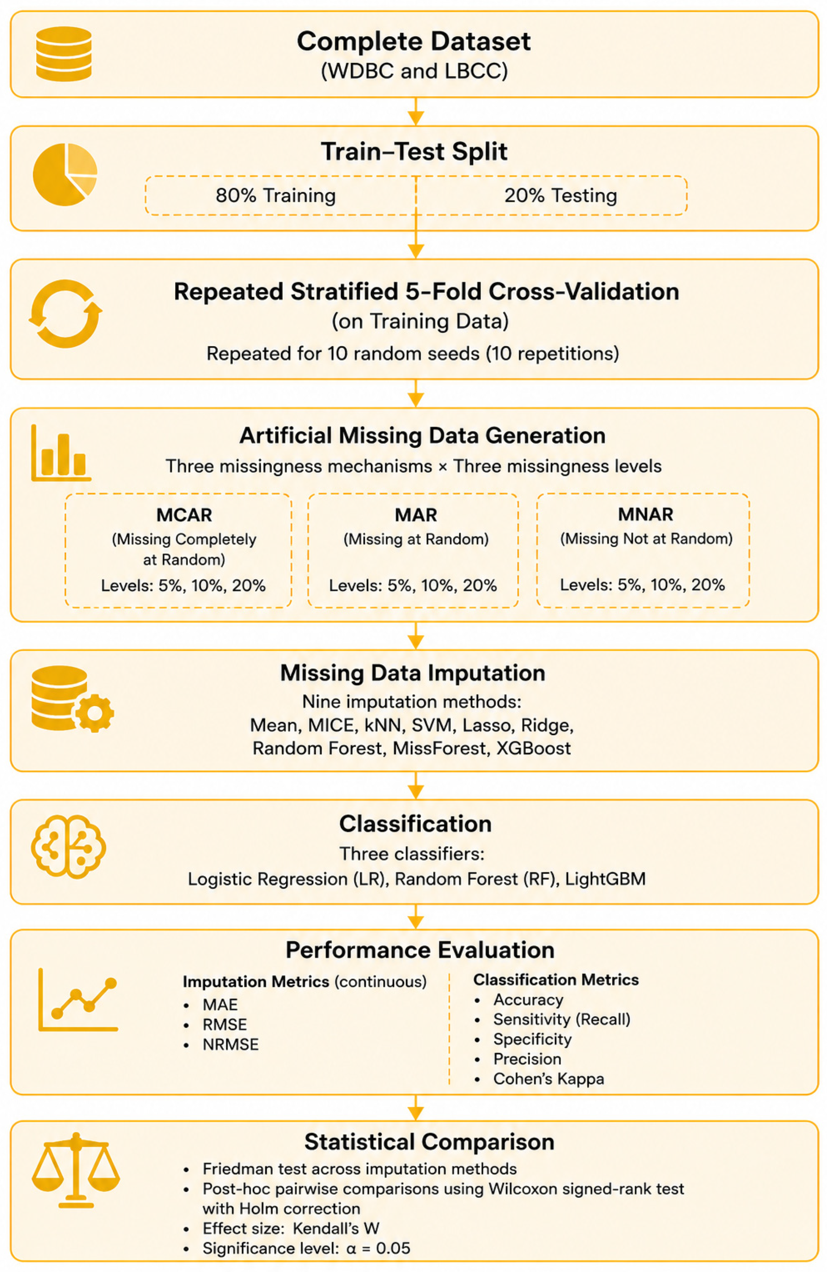
A simulation-based experimental framework was employed to evaluate the performance of statistical and machine learning-based imputation methods under controlled missing-data conditions. Complete reference datasets were first established for each breast cancer dataset, after which artificial missing values were introduced according to predefined missing-data mechanisms and proportions. The resulting incomplete datasets were subsequently imputed using the candidate imputation methods before downstream breast cancer classification was performed. The complete experimental pipeline, including missing-data generation, imputation, hyperparameter optimisation, model training and evaluation, was executed within a repeated stratified 5-fold nested cross-validation framework to minimise optimism bias and ensure reproducibility.

2.2.1. Artificial Missing Data Generation

Artificial missing values were generated exclusively in predictor variables, while the outcome variable remained fully observed throughout all experiments. This ensured that imputation performance could be evaluated against known reference values without introducing bias into the class labels. Missingness was simulated under the three mechanisms proposed by Rubin [15]: Missing Completely at Random (MCAR), Missing at Random (MAR), and Missing Not at Random (MNAR). Separate missingness patterns were generated independently for each dataset at 5%, 10% and 20% missingness [5]. The experimental workflow is shown in Figure 1.

In medical settings, incomplete data may arise from patient non-response, variations in diagnostic procedures, equipment limitations, or loss to follow-up. Understanding the mechanism underlying missingness is critical for selecting appropriate imputation methods and ensuring valid predictive modelling.

Let the complete dataset be denoted as:

$$Y=(Y_{obs},Y_{mis})$$

(1)

where $Y_{obs}$ represents observed values and $Y_{mis}$ represents missing values. Let $R$ be a missingness indicator matrix defined as:

$$R_{ij}=\left\{\begin{array}{cc}1,& \mathrm{if}{Y}_{ij}\mathrm{is}\mathrm{observed}\\ 0,& \mathrm{if}{Y}_{ij}\mathrm{is}\mathrm{missing}\end{array}\right.$$

The missing data mechanism is described by the conditional probability:

$$P(R=0\mid Y_{obs},Y_{mis},\theta )$$

where $\theta$ represents parameters governing the missingness process.

Missing Completely at Random (MCAR)

$$P(R=0\mid Y_{obs},Y_{mis},\theta )=P(R=0\mid \theta )$$

(2)

In breast cancer prediction, MCAR occurs when missing values arise independently of patient characteristics or disease status. For example, missing laboratory results due to random equipment failure or accidental data entry omissions would satisfy the MCAR assumption. Under MCAR, missing values were introduced independently of both observed and unobserved data. Predictor values were randomly selected with equal probability and replaced with missing values according to the predefined missingness proportion.

Missing at Random (MAR)

The probability of missingness was modelled using a logistic function:

$$P(R=0\mid Y_{obs},Y_{mis},\theta )=P(R=0\mid Y_{obs},\theta )$$

(3)

Implementation of Logistic Missingness Models.

Logistic missingness models were implemented using standardized predictor variables to improve numerical stability and ensure comparable effect sizes across variables. Continuous predictors entering the missingness models were standardized as

$$Z\left(X_i\right)={\displaystyle \frac{X_i-\overline{X}}{s_X}},$$

where $\overline{X}$ and $s_X$ denote the sample mean and standard deviation, respectively. For the WDBC dataset, MAR missingness was generated using two logistic models:

$$\mathrm{P}\mathrm{r}\left(R_{\mathrm{texture},i}=1\right)={\mathrm{l}\mathrm{o}\mathrm{g}\mathrm{i}\mathrm{t}}^{-1}\left({\alpha }_{\mathrm{texture}}+1.00\hspace{0.17em}Z\left({\mathrm{radius}\text{\_}\mathrm{mean}}_i\right)\right),$$

$$\mathrm{P}\mathrm{r}\left(R_{\mathrm{area},i}=1\right)={\mathrm{l}\mathrm{o}\mathrm{g}\mathrm{i}\mathrm{t}}^{-1}\left({\alpha }_{\mathrm{area}}+1.00\hspace{0.17em}Z\left({\mathrm{perimeter}\text{\_}\mathrm{mean}}_i\right)\right),$$

while MNAR missingness was generated as

$$\mathrm{P}\mathrm{r}\left(R_{\mathrm{texture},i}=1\right)={\mathrm{l}\mathrm{o}\mathrm{g}\mathrm{i}\mathrm{t}}^{-1}\left({\alpha }_{\mathrm{MNAR}}+1.00\hspace{0.17em}Z\left({\mathrm{texture}\text{\_}\mathrm{mean}}_i\right)\right).$$

For the LBCC dataset, MAR missingness in BMI was conditioned on standardized age, whereas missingness in 25-hydroxyvitamin D was conditioned jointly on Current Smoker and GRH Cohort. Specifically,

$$\mathrm{P}\mathrm{r}\left(R_{\mathrm{BMI},i}=1\right)={\mathrm{l}\mathrm{o}\mathrm{g}\mathrm{i}\mathrm{t}}^{-1}\left({\alpha }_{\mathrm{BMI}}+1.00\hspace{0.17em}Z\left({\mathrm{Age}}_i\right)\right),$$

$$\mathrm{P}\mathrm{r}\left(R_{25\mathrm{OHD},i}=1\right)={\mathrm{l}\mathrm{o}\mathrm{g}\mathrm{i}\mathrm{t}}^{-1}\left({\alpha }_{25\mathrm{OHD}}+0.75\hspace{0.17em}Z\left({\mathrm{Current}\mathrm{Smoker}}_i\right)+0.75\hspace{0.17em}Z\left({\mathrm{GRH}\mathrm{Cohort}}_i\right)\right).$$

Under MNAR, self-dependent missingness was induced using

$$\mathrm{P}\mathrm{r}\left(R_{\mathrm{BMI},i}=1\right)={\mathrm{l}\mathrm{o}\mathrm{g}\mathrm{i}\mathrm{t}}^{-1}\left({\alpha }_{\mathrm{BMI}}+1.00\hspace{0.17em}Z\left({\mathrm{BMI}}_i\right)\right),$$

and

$$\mathrm{P}\mathrm{r}\left(R_{25\mathrm{OHD},i}=1\right)={\mathrm{l}\mathrm{o}\mathrm{g}\mathrm{i}\mathrm{t}}^{-1}\left({\alpha }_{25\mathrm{OHD}}-1.00\hspace{0.17em}Z\left({25\mathrm{OHD}}_i\right)\right),$$

where $R_i=1$ indicates that the corresponding observation was set to missing.

MAR is more realistic in clinical settings. In breast cancer prediction, missingness often depends on observed variables such as age, tumour size, or stage of diagnosis. For instance, certain diagnostic tests (e.g., advanced imaging or biomarker assays) may be more likely to be conducted for patients with severe or suspicious clinical presentations. Thus, the probability of missing data in specific variables can be explained by other observed patient characteristics. Most statistical and machine learning imputation methods, including Multiple Imputation by Chained Equations (MICE), Random Forest-based imputation, and gradient boosting approaches, rely on the MAR assumption. When this assumption holds and relevant predictors are included, unbiased estimation and reliable prediction are achievable.

To simulate realistic clinical scenarios, missingness was induced using clinically plausible relationships between predictors. For the WDBC dataset, missingness was generated using highly correlated morphometric features. For example, the probability of missing values in texture_mean depended on the observed value of radius_mean, while missingness in area_mean depended on perimeter_mean. These relationships reflect the strong biological correlations among tumour morphology characteristics. For the LBCC dataset, missingness was generated using observed demographic and clinical characteristics. Specifically, missingness in 25-hydroxyvitamin D measurements was modelled as a function of Age, missingness in BMI depended on Current Smoker status, and missingness in Calcium depended on Cohort membership, representing differences in participant characteristics and data collection protocols commonly encountered in longitudinal studies.

Intercept Calibration and Missingness Generation.

For each predefined missingness proportion (5%, 10%, and 20%), the logistic intercept ($\alpha$) was numerically calibrated so that the expected average probability of missingness equalled the target rate. The intercept was obtained by solving

$${\displaystyle \frac{1}{n}}{\displaystyle \sum _{i=1}^n}{\mathrm{l}\mathrm{o}\mathrm{g}\mathrm{i}\mathrm{t}}^{-1}\left(\alpha +{\eta }_i\right)=q,$$

where $q$ denotes the target missingness proportion and ${\eta }_i$ represents the linear predictor for observation $i$. Calibration was performed using the base R function uniroot() over the interval $[-30,30]$ with a numerical tolerance of ${10}^{-12}$. Missingness indicators were subsequently generated as independent Bernoulli random variables using the calibrated probabilities. Consequently, the expected proportion of missing values matched the target level, while the realised proportion varied slightly across random seeds because of stochastic sampling.

Missing Not at Random (MNAR)

$$P\left(R=0∣Y_{obs},Y_{mis},\theta \right)=P(R=0\mid Y_{obs},Y_{mis},\theta )$$

(4)

MNAR arises when missingness depends on unobserved values, which is common in sensitive or clinically severe cases. In breast cancer prediction, patients with advanced disease or poor prognosis may be less likely to complete follow-up assessments or undergo certain diagnostic procedures. Similarly, missing genomic or biomarker data may occur more frequently in cases where tumour characteristics are extreme or difficult to measure. Under MNAR, the missingness mechanism is non-ignorable, and standard imputation techniques may lead to biased estimates because the missing values are systematically related to the unobserved data. Addressing MNAR typically requires specialized modelling approaches or sensitivity analysis.

Under MNAR, missingness depended on the value of the variable itself. Logistic missingness models were used to generate self-dependent missingness. For the WDBC dataset, larger values of selected morphometric features (e.g., texture_mean) were assigned progressively higher probabilities of becoming missing. For the LBCC dataset, missingness was induced directly within clinically relevant variables, including BMI and 25-hydroxyvitamin D, such that participants with extreme values were more likely to have missing observations. This reflects situations frequently encountered in biomedical research where the likelihood of a measurement being missing depends on its underlying value.

Artificial missing values were introduced only into continuous predictor variables. For the WDBC dataset, missingness was induced in continuous morphometric features, whereas for the LBCC dataset, missingness was induced only in BMI and 25-hydroxyvitamin D. The categorical variables Current Smoker and GRH Cohort were used solely as conditioning variables within the MAR logistic models and were never subjected to artificial missingness. Consequently, MAE, RMSE, and NRMSE were computed exclusively for continuous variables with induced missing values.

2.2.2. Implications for Breast Cancer Prediction Models

In breast cancer prediction, the choice of imputation method is closely tied to assumptions about the missing data mechanism. While MCAR provides an ideal but rare scenario, MAR is commonly assumed in practice and forms the basis for most imputation techniques. However, the presence of MNAR can significantly degrade model performance, particularly in high-stakes clinical predictions where missingness may be linked to disease severity. Therefore, robust evaluation of imputation methods across MCAR, MAR, and MNAR scenarios is essential to ensure that predictive models remain reliable under realistic clinical conditions.

2.3. Imputation Models

Missing value imputation in this study is formulated as a statistical learning problem in which the objective is to estimate the unobserved components of a data matrix using the observed information. Let $X\in {\mathbb{R}}^{n\times p}$ denote the dataset with missing entries, partitioned as $X=(X_{obs},X_{mis})$. The imputation problem consists of estimating $X_{mis}$ through a mapping:

$${\widehat{X}}_{mis}=\mathcal{F}(X_{obs};\Theta ),$$

(5)

where $\mathcal{F}$ represents the imputation model and $\Theta$ denotes its parameters.

From a probabilistic perspective, the optimal imputation under squared error loss corresponds to the conditional expectation:

$${\widehat{X}}_{mis}=\mathbb{E}[X_{mis}\mid X_{obs}],$$

(6)

which is generally unknown and must be approximated using statistical or machine learning models. The methods employed in this study can be interpreted as different approximations to this conditional expectation, each imposing distinct structural assumptions on the data-generating process. The selection of the methods was based on a prior study by Nyakundi et al. [8] that systematically explored the application of machine learning methods in breast cancer prediction.

2.3.1. Statistical Models

i.

Mean Imputation

Mean imputation represents the simplest estimator, replacing missing values with the marginal expectation:

$${\widehat{x}}_{ij}=\mathbb{E}[X_j]\approx {\displaystyle \frac{1}{n_j}}\sum _{i\in {\mathcal{O}}_j}{x}_{ij}.$$

(7)

This approach assumes independence among variables and ignores the joint distribution $P(X)$. Consequently, it underestimates variance and distorts covariance structure:

$$\mathrm{Var}({\tilde{X}}_j)<\mathrm{Var}(X_j),\mathrm{Cov}({\tilde{X}}_j,{\tilde{X}}_k)\to 0.$$

(8)

ii.

MultipleImputation by Chained Equations (MICE)

MICE adopts a Fully Conditional Specification (FCS) framework, modelling each variable conditionally on all others:

$$X_j\mid X_{-j}\sim f_j(X_{-j};{\theta }_j).$$

(9)

Imputation proceeds iteratively:

$$X_j^{(t)}\sim P(X_j\mid X_{-j}^{(t-1)},{\theta }_j),$$

(10)

forming a Markov chain whose stationary distribution approximates the joint distribution $P(X)$.

MICE is asymptotically valid under MAR and correct model specification. Its strength lies in capturing multivariate dependence, although it is sensitive to model misspecification.

2.3.2. Distance-Based Models

iii.

k-Nearest Neighbors (kNN)

kNN imputation is a nonparametric method that estimates missing values through local averaging:

$${\widehat{x}}_{ij}=\sum _{l\in {\mathcal{N}}_k(i)}{w}_{il}{x}_{lj},w_{il}\propto {\displaystyle \frac{1}{d(x_i,x_l)}}.$$

(11)

This method approximates the conditional expectation via a kernel smoother:

$${\widehat{x}}_{ij}\approx \mathbb{E}[X_j\mid X_{-j}\in {\mathcal{N}}_k(x_i)].$$

(12)

Its performance depends critically on the distance metric and the choice of $k$.

2.3.3. Kernel-Based Models

iv.

Support Vector Machine (SVM)

SVM imputation treats missing value estimation as a regression problem in a reproducing kernel Hilbert space (RKHS). The model is:

$$f(x)=w^{\mathrm{\top }}\varphi (x)+b,$$

(13)

where $\varphi (x)$ is an implicit feature mapping induced by a kernel $K(x_i,x_j)$.

The optimization problem is:

$$\underset{w,b}{\mathrm{m}\mathrm{i}\mathrm{n}}{\displaystyle \frac{1}{2}}\parallel w{\parallel }^2+C{\displaystyle \sum _{i=1}^n}\mathrm{m}\mathrm{a}\mathrm{x}(0,\mid y_i-f(x_i)\mid -ϵ).$$

(14)

This yields a flexible nonlinear estimator of:

$${\widehat{x}}_{ij}\approx \mathbb{E}[X_j\mid X_{-j}],$$

(15)

with regularization controlling overfitting.

2.3.4. Tree-Based Ensemble Models

v.

Random Forest

Random Forest approximates the conditional expectation using an ensemble of decision trees:

$${\widehat{x}}_{ij}={\displaystyle \frac{1}{T}}{\displaystyle \sum _{t=1}^T}{f}_t(x_i^{(-j)}),$$

(16)

where each tree $f_t$ is trained on a bootstrap sample with random feature selection.

RF is a consistent, nonparametric estimator under certain conditions and captures complex interactions without requiring parametric assumptions.

vi.

MissForest

MissForest extends RF into an iterative imputation framework. Starting with an initial guess $X^{\left(0\right)}$, updates are defined as:

$$X_{mis}^{\left(t\right)}={\mathcal{F}}_{RF}(X_{obs},X_{mis}^{\left(t−1\right)}).$$

(17)

The procedure iteratively refines imputations until convergence, effectively performing a fixed-point iteration:

$$X^{\ast }={\mathcal{F}}_{RF}(X^{\ast }).$$

(18)

MissForest is particularly effective for mixed-type data and complex nonlinear dependencies.

vii. 

Extreme Gradient Boosting (XGBoost)

XGBoost constructs an additive model:

$${\widehat{y}}_i={\displaystyle \sum _{k=1}^K}{f}_k(x_i),$$

(19)

by minimizing:

$$\mathcal{L}={\displaystyle \sum _{i=1}^n}\mathcal{l}(y_i,{\widehat{y}}_i)+{\displaystyle \sum _{k=1}^K}\Omega (f_k),$$

(20)

with:

$$\Omega (f_k)=\gamma T_k+{\displaystyle \frac{1}{2}}\lambda \parallel w_k{\parallel }^2.$$

(21)

Missing values are handled internally by assigning optimal default directions during tree splitting, effectively learning:

$${\widehat{x}}_{ij}=\mathrm{a}\mathrm{r}\mathrm{g} \underset{split}{\mathrm{m}\mathrm{i}\mathrm{n}}\hspace{0.25em} \mathcal{L}.$$

(22)

This allows XGBoost to integrate imputation within model training, yielding strong performance in structured datasets.

2.3.5. Regularized Regression Models

viii.

Lasso Regression

Lasso solves:

$$\widehat{\beta }=\mathrm{a}\mathrm{r}\mathrm{g} \underset{\beta }{\mathrm{m}\mathrm{i}\mathrm{n}}\left\{\parallel y-X\beta {\parallel }^2+\lambda \parallel \beta {\parallel }_1\right\}.$$

(23)

The L1 penalty induces sparsity:

$${\beta }_j=0\mathrm{for}\mathrm{irrelevant}\mathrm{predictors},$$

making Lasso suitable for variable selection and imputation.

ix.

Ridge Regression

Ridge regression solves:

$$\widehat{\beta }=\mathrm{a}\mathrm{r}\mathrm{g} \underset{\beta }{\mathrm{m}\mathrm{i}\mathrm{n}}\left\{\parallel y-X\beta {\parallel }^2+\lambda \parallel \beta {\parallel }_2^2\right\},$$

(24)

with solution:

$$\widehat{\beta }=(X^{\mathrm{\top }}X+\lambda I{)}^{-1}{X}^{\mathrm{\top }}y.$$

(25)

Ridge stabilizes estimates under multicollinearity and provides smooth approximations of the conditional expectation.

2.3.6. Repeated Nested Cross-Validation

Model development and evaluation were conducted using a repeated stratified 5-fold nested cross-validation framework. During each repetition, the datasets were partitioned into five folds while preserving the distribution of the outcome classes. For the LBCC dataset, all observations from the same participant were allocated to the same fold to maintain the longitudinal structure and prevent information leakage. Within each outer training fold, artificial missing values were generated, followed by imputation using the candidate methods. Hyperparameter optimisation for each classification algorithm was subsequently performed using only the corresponding inner training data. The optimised model was then evaluated on the unseen outer test fold. To improve the stability and reproducibility of the results, the complete experimental pipeline—including data partitioning, missing-data generation, imputation, hyperparameter optimisation, model training and evaluation—was repeated 10 times using different random seeds. Performance metrics were averaged across all repetitions, and their corresponding standard deviations were reported.

Table 2. Summary of artificial missing-data generation.

Dataset	Mechanism	Variable(s) with Induced Missingness	Missingness Conditioned on	Simulation Assumptions
WDBC	MCAR	All predictor variables	Random selection	Missing values occur completely at random, representing data entry errors, transmission failures or random measurement omissions unrelated to tumour characteristics.
WDBC	MAR	texture_mean, area_mean	radius_mean, perimeter_mean	Missingness in selected morphometric features is assumed to depend on other observed tumour characteristics because these variables are highly correlated and jointly describe tumour morphology.
WDBC	MNAR	texture_mean	texture_mean	Missingness is assumed to increase with extreme values of texture_mean, representing clinically plausible scenarios in which complex tumour morphology may lead to segmentation difficulties or measurement uncertainty, making missingness dependent on the underlying value itself.
LBCC	MCAR	All predictor variables	Random selection	Missing values occur randomly because of recording errors or incidental omissions during follow-up, independent of participant characteristics.
LBCC	MAR	25(OH)D, BMI, Calcium	Age, Current Smoker, Cohort	Missingness is assumed to depend on observed participant characteristics and study design factors, reflecting differences in laboratory testing, follow-up attendance and data collection protocols across cohorts.
LBCC	MNAR	25(OH)D, BMI	Variable’s own value	Missingness is assumed to increase for extreme vitamin D concentrations and BMI values, representing plausible biomedical scenarios in which the probability of observing a measurement depends on the participant’s underlying physiological status rather than only the observed covariates.

summarizes the missing data generation and underlying assumptions.

Artificial missing-data generation and imputation evaluation were performed independently across ten missingness seeds (101, 202, 303, 404, 505, 606, 707, 808, 909, and 1010). The resulting imputation performance metrics (MAE, RMSE, and NRMSE) were therefore summarised across all simulated datasets. In contrast, downstream breast cancer classification was conducted using the representative imputed datasets generated with seed 101. This design separated the comprehensive evaluation of imputation performance from the computationally intensive classification analyses while maintaining a consistent downstream validation framework.

The variables selected to induce MAR and MNAR mechanisms were chosen to reflect clinically plausible dependency structures while ensuring reproducibility of the simulation framework across datasets. These assumptions were introduced solely for simulation purposes and should not be interpreted as reflecting the true missing-data mechanisms in the original datasets.

Table 3. (A). Implementation settings for the evaluated imputation methods. (B). Hyperparameter optimization settings for the evaluated classification models.

(A)
Method	R Package (Version)	Hyperparameter(s)	Configuration Used	Tuning Strategy
Mean	base R (4.6.1)	None	Mean of each predictor calculated from the available observations	Not applicable
MICE	mice (3.19.0)	Imputation method; number of imputations; iterations	Predictive mean matching; m = 5; maxit = 10	Fixed predefined settings
kNN	VIM (7.0)	Number of neighbours (k)	k = 5	Fixed predefined setting
SVM regression	e1071 (1.7-17)	Kernel; cost; gamma; epsilon	Radial kernel; cost = 1; gamma = 1/p (package default); epsilon = 0.1	Fixed predefined settings
Lasso	glmnet (5.0)	Regularization parameter (λ)	Lambda selected from the automatically generated glmnet sequence	Internal 5-fold cross-validation using cv.glmnet
Ridge	glmnet (5.0)	Regularization parameter (λ)	Lambda selected from the automatically generated glmnet sequence	Internal 5-fold cross-validation using cv.glmnet
Random Forest	randomForest (4.7-1.2)	Number of trees; mtry; minimum node size	ntree = 200; mtry = √p; minimum node size = 5	Fixed predefined settings
MissForest	missForest (1.6.1)	Maximum iterations; convergence tolerance	Maximum iterations = 5; tolerance = 0.001	Iterative fitting until convergence or maximum iterations
XGBoost	xgboost (3.2.1.1)	Number of rounds; learning rate; maximum depth; subsampling parameters; minimum child weight	nrounds = 150; eta = 0.05; max_depth = 4; subsample = 0.80; colsample_bytree = 0.80; min_child_weight = 1	Fixed predefined settings
(B)
Classifier	R Package (Version)	Hyperparameter(s)	Tuning Space	Selection Criterion
Logistic Regression (LR)	stats (4.6.1)	None	Not applicable	No hyperparameter tuning
Random Forest (RF)	randomForest (4.7-1.2)	ntree, mtry, nodesize	ntree ∈ {200, 500, 1000}; mtry ∈ {⌊√p/2⌋, ⌊√p⌋, ⌊2√p⌋}; nodesize ∈ {1, 5, 10}	Mean validation AUC within the inner cross-validation loop
LightGBM	lightgbm (4.7.0)	num_iterations, learning_rate, max_depth, num_leaves, min_data_in_leaf, bagging_fraction, feature_fraction, lambda_l1, lambda_l2	num_iterations ∈ {100, 200, 500}; learning_rate ∈ {0.01, 0.05, 0.10}; max_depth ∈ {−1, 3, 5, 7}; num_leaves ∈ {7, 15, 31, 63}; min_data_in_leaf ∈ {10, 20, 40}; bagging_fraction ∈ {0.70, 0.85, 1.00}; feature_fraction ∈ {0.70, 0.85, 1.00}; lambda_l1 ∈ {0, 0.1, 1}; lambda_l2 ∈ {0, 0.1, 1}	Mean validation AUC within the inner cross-validation loop with early stopping

Note for (A): Artificial missing-data generation was repeated using 10 independent random seeds (101, 202, 303, 404, 505, 606, 707, 808, 909 and 1010) for each missingness mechanism (MCAR, MAR and MNAR) and missingness level (5%, 10% and 20%). Imputation performance was evaluated using MAE, RMSE and NRMSE across all simulated datasets. Note for (B): Artificial missing-data generation and imputation performance evaluation were conducted across ten independent missingness seeds (101–1010). Downstream classification was subsequently performed using the representative imputed datasets generated with seed 101. All preprocessing, imputation, Borderline-SMOTE (LBCC only), hyperparameter optimisation, and classifier fitting were performed exclusively within the training folds to prevent information leakage.

A,B summarizes the implementation details and hyperparameter settings for the evaluated imputation methods, including the software package, key hyperparameters, search space or predefined settings, tuning strategy, and training-fold implementation. Methods requiring minimal user specification were implemented using established settings, whereas tunable algorithms were optimised within the training folds.

2.4. Performance Evaluation and Comparison of Imputation Methods

Evaluation of Imputation Performance

The evaluation of imputation performance was conducted by comparing imputed values with their corresponding true values in the reference (complete-case) dataset. Let $X\in {\mathbb{R}}^{n\times p}$ denote the complete data matrix and $\mathcal{M}=\{(i,j):R_{ij}=0\}$ the index set of entries that were artificially set to missing. Let $x_{ij}$ denote the true value and ${\widehat{x}}_{ij}$ the imputed value. All performance metrics were computed over $\mathcal{M}$, thereby isolating the accuracy of the imputation procedure.

From a statistical perspective, imputation accuracy can be interpreted as an empirical estimate of the risk associated with an estimator ${\widehat{X}}_{mis}$ of the target quantity $X_{mis}$. Under a loss function $L({\widehat{x}}_{ij},x_{ij})$, the expected risk is:

$$\mathcal{R}=\mathbb{E}\left[L({\widehat{x}}_{ij},x_{ij})\right],$$

(26)

which is approximated using sample-based error metrics. In this study, three complementary metrics were employed: Root Mean Square Error (RMSE), Mean Absolute Error (MAE), and Normalized Root Mean Square Error (NRMSE).

i.

Root Mean Square Error (RMSE)

RMSE is defined as:

$$\mathrm{RMSE}={\left({\displaystyle \frac{1}{\mid \mathcal{M}\mid }}\sum _{(i,j)\in \mathcal{M}}({\widehat{x}}_{ij}-x_{ij}{)}^2\right)}^{1/2}$$

(27)

RMSE corresponds to the empirical $L_2$ risk and is directly linked to the mean squared error:

$$\mathrm{MSE}=\mathbb{E}[({\widehat{x}}_{ij}-x_{ij}{)}^2].$$

(28)

It penalizes large deviations quadratically and is therefore sensitive to heavy-tailed error distributions. In the context of imputation, RMSE is particularly informative when large imputation errors have disproportionate effects on downstream analyses, such as classification model instability.

ii.

Mean Absolute Error (MAE)

MAE is defined as:

$$\mathrm{MAE}={\displaystyle \frac{1}{\mid \mathcal{M}\mid }}\sum _{(i,j)\in \mathcal{M}}\mid {\widehat{x}}_{ij}-x_{ij}\mid$$

(29)

MAE represents the empirical $L_1$ risk:

$$\mathbb{E}[\mid {\widehat{x}}_{ij}-x_{ij}\mid ],$$

(30)

and provides a robust measure of central tendency of the error distribution. Unlike RMSE, MAE is less sensitive to extreme values and is therefore preferable when the imputation error distribution is skewed or contains outliers.

iii.

Normalized Root Mean Square Error (NRMSE)

To enable comparability across variables with differing scales and variances, RMSE was normalized. The NRMSE is defined as:

$$\mathrm{NRMSE}={\left({\displaystyle \frac{\sum _{(i,j)\in \mathcal{M}}({\widehat{x}}_{ij}-x_{ij}{)}^2}{\sum _{(i,j)\in \mathcal{M}}(x_{ij}-{\bar{x}}_j{)}^2}}\right)}^{1/2}$$

(31)

where ${\bar{x}}_j={\displaystyle \frac{1}{n_j}}{\sum }_{i\in {\mathcal{O}}_j}{x}_{ij}$ is the sample mean of observed values for variable $j$.

NRMSE can be interpreted as a scale-free measure of relative error:

$$\mathrm{NRMSE}\approx {\displaystyle \frac{\sqrt{\mathrm{MSE}}}{\mathrm{SD}(X_j)}},$$

(32)

allowing comparison across variables and datasets with heterogeneous distributions. It is particularly useful in multivariate settings where variables differ in magnitude or dispersion.

2.5. Evaluation of Classification Performance

After imputation, classification models were constructed using the imputed datasets to evaluate the impact of the imputation methods on breast cancer diagnostic performance. Five performance metrics were used for this purpose: Accuracy, Sensitivity, Specificity, Precision, and Cohen’s Kappa statistic.

2.5.1. Classification Models

To evaluate the impact of different imputation strategies on downstream breast cancer classification, three complementary classifiers were employed: Logistic Regression (LR), Random Forest (RF), and Light Gradient Boosting Machine (LightGBM). These algorithms represent statistical learning, bagging-based ensemble learning, and gradient boosting paradigms, respectively, providing increasing modelling complexity and enabling assessment of whether the effectiveness of the imputation methods is consistent across different classification approaches.

• Logistic Regression (LR)

Logistic Regression estimates the probability that an observation belongs to the malignant class using the logistic function

$$\begin{array}{cccc}& P(Y=1\mid X)={\displaystyle \frac{1}{1+\mathrm{e}\mathrm{x}\mathrm{p}\left[-({\beta }_0+{\beta }^{T}X)\right]}},& & \end{array}$$

(33)

where $X$ denotes the predictor vector, ${\beta }_0$ is the intercept, and $\beta$ represents the regression coefficients estimated by maximum likelihood. LR provides a simple and interpretable statistical baseline against which the performance of more complex ensemble classifiers can be evaluated.

ii.

Random Forest

Random Forest is an ensemble learning algorithm that combines multiple decision trees constructed using bootstrap samples and random feature selection. The final prediction is obtained through majority voting,

$$\begin{array}{cccc}& \widehat{y}=\mathrm{m}\mathrm{o}\mathrm{d}\mathrm{e}\left\{f_1(x),f_2(x),\dots ,f_T(x)\right\},& & \end{array}$$

(34)

where $f_t(x)$ denotes the prediction from the $t^{\mathrm{th}}$ decision tree and $T$ is the total number of trees in the ensemble. RF captures nonlinear relationships and higher-order feature interactions without requiring parametric assumptions. Its ensemble structure also improves robustness to noisy predictors and overfitting, making it a suitable benchmark for structured biomedical datasets.

iii.

Light Gradient Boosting Machine

LightGBM is a gradient boosting algorithm that constructs an additive ensemble of decision trees,

$$\begin{array}{cccc}& {\widehat{y}}_i={\displaystyle \sum _{k=1}^K}{f}_k(x_i),& & \end{array}$$

(35)

where $f_k(·)$ represents the prediction from the $k^{\mathrm{th}}$ boosting tree. Model parameters are estimated by minimizing the regularized objective function

$$\begin{array}{cccc}& L={\displaystyle \sum _{i=1}^n}l(y_i,{\widehat{y}}_i)+{\displaystyle \sum _{k=1}^K}\Omega (f_k),& & \end{array}$$

(36)

where $l(·)$ is the classification loss function and $\Omega (f_k)$ penalizes model complexity. LightGBM was selected because previous work by Nyakundi et al. [8] demonstrated its strong predictive performance for breast cancer prediction. Its histogram-based learning and leaf-wise tree growth provide high predictive accuracy while maintaining computational efficiency for structured biomedical datasets.

iv.

Model Development

Model development was embedded within the repeated stratified 5-fold nested cross-validation framework described above. For each outer training fold, missing values were first imputed using the selected imputation method, after which classifier hyperparameters were optimized within the corresponding inner cross-validation loop. The optimized models were subsequently retrained on the complete outer training fold and evaluated on the unseen outer test fold. This procedure ensured that encoding, imputation, hyperparameter optimisation, and classifier training were performed independently within each training fold, thereby preventing information leakage. Because the LBCC dataset was severely imbalanced, Borderline-SMOTE was applied exclusively to the analysis portion of each inner cross-validation fold during hyperparameter tuning. Inner validation folds and outer test folds retained their original class distributions. After selection of the optimal hyperparameters, Borderline-SMOTE was applied to the complete outer training fold before fitting the final classifier.

2.5.2. Classification Performance Metrics

Classification performance was evaluated using Accuracy, Sensitivity, Specificity, Precision, and Cohen’s Kappa.

• Sensitivity

Sensitivity measures the ability of the classification model to correctly identify malignant/BC cases. In clinical diagnostic applications, sensitivity is a critical metric because failing to detect malignant/BC cases may lead to delayed treatment and severe health consequences.

Sensitivity is defined as:

$$\mathrm{S}\mathrm{e}\mathrm{n}\mathrm{s}\mathrm{i}\mathrm{t}\mathrm{i}\mathrm{v}\mathrm{i}\mathrm{t}\mathrm{y}={\displaystyle \frac{\mathrm{T}\mathrm{P}}{\mathrm{T}\mathrm{P}+\mathrm{F}\mathrm{N}}}$$

(37)

where $TP$ represents the number of true positive cases correctly classified as malignant/BC cases, and $FN$ represents the number of false negative cases where malignant/BC cases are incorrectly classified as benign/non-BC cases.

A higher sensitivity indicates that the diagnostic model is more effective in detecting malignant/BC cases.

ii.

Accuracy

Accuracy measures the overall proportion of correctly classified observations and is defined as

$$\mathrm{A}\mathrm{c}\mathrm{c}\mathrm{u}\mathrm{r}\mathrm{a}\mathrm{c}\mathrm{y}={\displaystyle \frac{\mathrm{T}\mathrm{P}+\mathrm{T}\mathrm{N}}{\mathrm{T}\mathrm{P}+\mathrm{T}\mathrm{N}+\mathrm{F}\mathrm{P}+\mathrm{F}\mathrm{N}}}.$$

(38)

Although accuracy provides an overall measure of predictive performance, it should be interpreted together with sensitivity and specificity, particularly when class distributions are imbalanced.

iii.

Cohen’s Kappa Statistic

The Cohen’s Kappa statistic was used to assess the agreement between the predicted classification results and the true diagnostic labels while accounting for agreement occurring by chance. The Kappa statistic is defined as:

$$\mathrm{K}\mathrm{a}\mathrm{p}\mathrm{p}\mathrm{a}={\displaystyle \frac{{\mathrm{p}}_{\mathrm{o}}-{\mathrm{p}}_{\mathrm{e}}}{1-{\mathrm{p}}_{\mathrm{e}}}}$$

(39)

where $p_o$ represents the observed agreement, and $p_e$ represents the expected agreement by chance.

Higher Kappa values indicate stronger agreement between predicted and actual outcomes and therefore greater reliability of the classification model.

iv.

Specificity

Specificity measures the ability of a classifier to correctly identify negative cases (benign tumors/non-BC cases) and is particularly important for minimizing false-positive diagnoses in breast cancer screening. It is defined as the proportion of true negatives among all actual negative cases:

$$\mathrm{Specificity}={\displaystyle \frac{\mathrm{T}\mathrm{N}}{\mathrm{T}\mathrm{N}+\mathrm{F}\mathrm{P}}},$$

(40)

where $TN$ and $FP$ denote the numbers of true negatives and false positives, respectively. Higher specificity indicates better discrimination of benign cases, reducing unnecessary follow-up investigations and improving the clinical utility of the diagnostic model.

v.

Precision

Precision measures the ability of a classifier to correctly identify positive cases by quantifying the proportion of predicted positive cases that are truly positive. It is particularly important in breast cancer diagnosis because it minimizes false-positive predictions, thereby reducing unnecessary diagnostic procedures and patient anxiety. It is defined as the proportion of true positives among all cases predicted as positive:

$$\mathrm{Precision}={\displaystyle \frac{\mathrm{T}\mathrm{P}}{\mathrm{T}\mathrm{P}+\mathrm{F}\mathrm{P}}},$$

(41)

where $TP$ and $FP$ denote the numbers of true positives and false positives, respectively. Higher precision indicates that a greater proportion of patients classified as having breast cancer are correctly diagnosed, enhancing the reliability and clinical usefulness of the diagnostic model.

2.6. Statistical Significance Testing

Statistical analyses were conducted to determine whether differences in imputation performance among the evaluated methods were statistically significant across repeated experiments. Since performance measures did not necessarily satisfy the assumptions of normality and homoscedasticity, non-parametric statistical tests were employed. The experimental unit for all statistical analyses was one independently generated incomplete dataset. Each unit corresponded to a unique combination of missingness mechanism (MCAR, MAR, or MNAR), missingness level (5%, 10%, or 20%), and random seed. Imputation performance metrics obtained from the nine imputation methods were compared within these predefined experimental conditions.

The Friedman test was first used to compare the imputation methods across multiple experimental conditions using average ranks. The Friedman statistic is given by

$$\begin{array}{cccc}& {\chi }_F^2={\displaystyle \frac{12N}{k(k+1)}}\left[{\displaystyle {\sum }_{j=1}^k}{R}_j^2−{\displaystyle \frac{k(k+1{)}^2}{4}}\right],& & \end{array}$$

(42)

where $N$ is the number of experimental runs, $k$ is the number of imputation methods, and $R_j$ is the average rank of the $j^{th}$ method. A significant Friedman test indicates that at least one imputation method differs from the others. Complete Friedman test results for each dataset, missingness mechanism, and missingness level are presented in Appendix A and Appendix B.

When the Friedman test was significant ($p<0.05$), pairwise comparisons were performed using the Wilcoxon signed-rank test with Holm’s correction to control the family-wise error rate associated with multiple comparisons. Effect sizes were quantified using the rank-biserial correlation to assess the magnitude of pairwise differences. Mean performance values across the repeated simulation experiments were reported to quantify both predictive performance and variability. All statistical tests were two-sided and conducted at a significance level of 5%.

3. Results

The imputation and classification performance of the proposed framework was evaluated using the WDBC and LBCC datasets. One of the earliest and most common signs of breast cancer is the detection of a breast lump or abnormal growth. Such a lump may be either malignant (cancerous) or benign (non-cancerous), making prompt medical evaluation essential for an accurate diagnosis. Since the WDBC dataset exhibited a balanced class distribution, no additional class balancing was required. In contrast, the minority class in the LBCC dataset was balanced using the Borderline Synthetic Minority Oversampling Technique (BSMOTE) during model training to minimise classification bias. The analyses were conducted across the different missing-data mechanisms and missingness levels described in the methodology. The results are presented in three stages: first, the performance of the imputation methods is evaluated using reconstruction error metrics; second, statistical comparisons among the imputation methods are presented; and finally, the classification performance of the best-performing imputation methods is assessed using three machine learning classifiers.

3.1. Imputation Performance

3.1.1. Imputation Performance on the WDBC Dataset

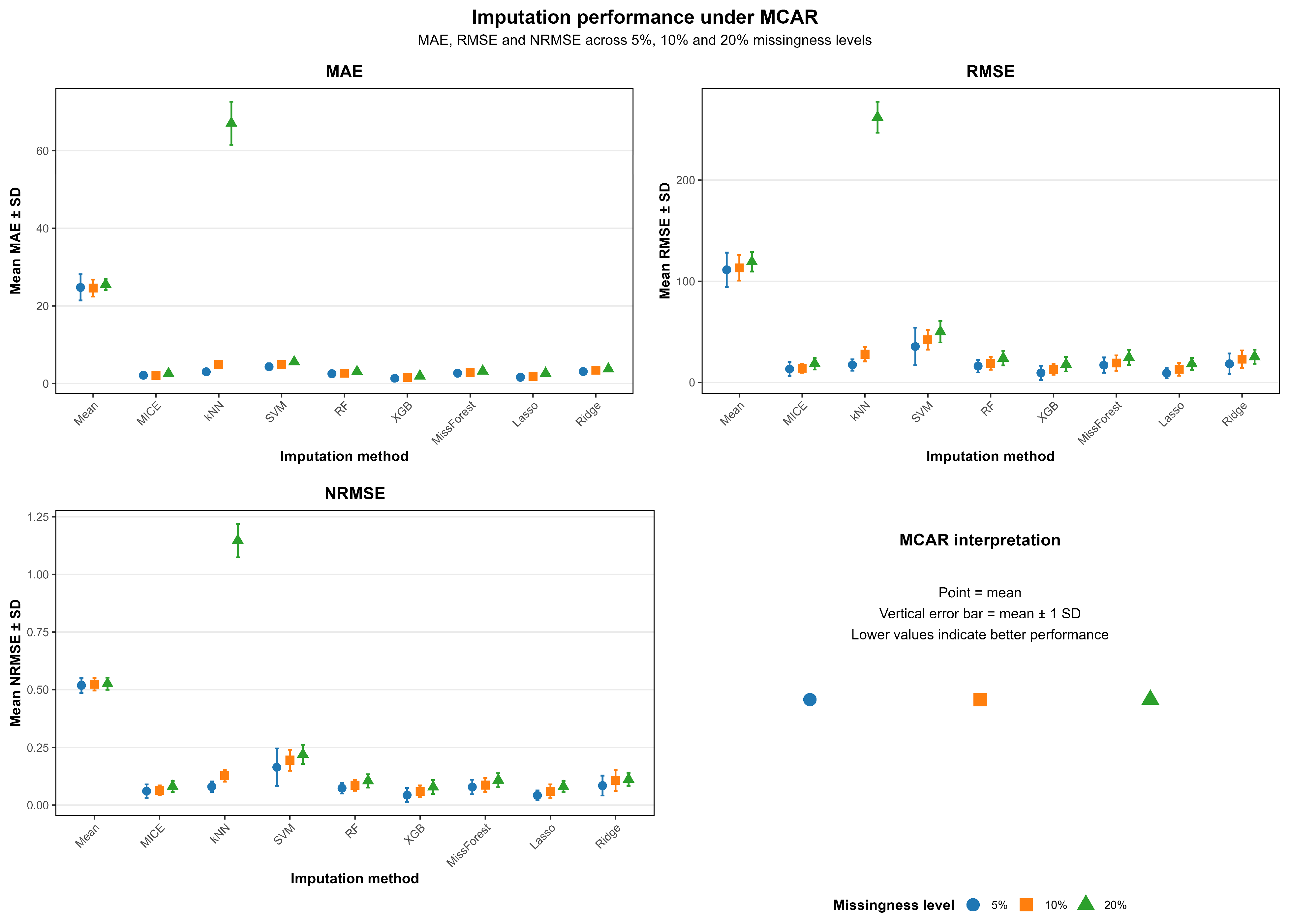
To evaluate the robustness of the imputation methods on the WDBC dataset, average imputation performance was compared across MCAR, MAR, and MNAR missingness mechanisms at 5%, 10%, and 20% missingness levels using MAE, RMSE, and NRMSE as performance metrics. Across the three missingness mechanisms, the imputation models exhibited distinct performance patterns. Under MCAR, most machine learning and regularized regression methods maintained relatively low prediction errors, with Lasso and XGBoost (XGB) consistently emerging as the strongest performers across MAE, RMSE, and NRMSE. MICE also demonstrated competitive performance, particularly at lower levels of missingness, while Random Forest (RF), MissForest, Ridge, and kNN generally produced intermediate results. In contrast, the simple mean imputation method consistently performed worst, reflecting its inability to preserve the multivariate relationships within the WDBC data. As the proportion of missing data increased, all methods experienced some deterioration in performance; however, Lasso and XGB remained comparatively robust, whereas kNN showed a marked decline at the highest missingness level, suggesting reduced stability under extensive information loss. The imputation performance under MCAR is given in Figure 2.

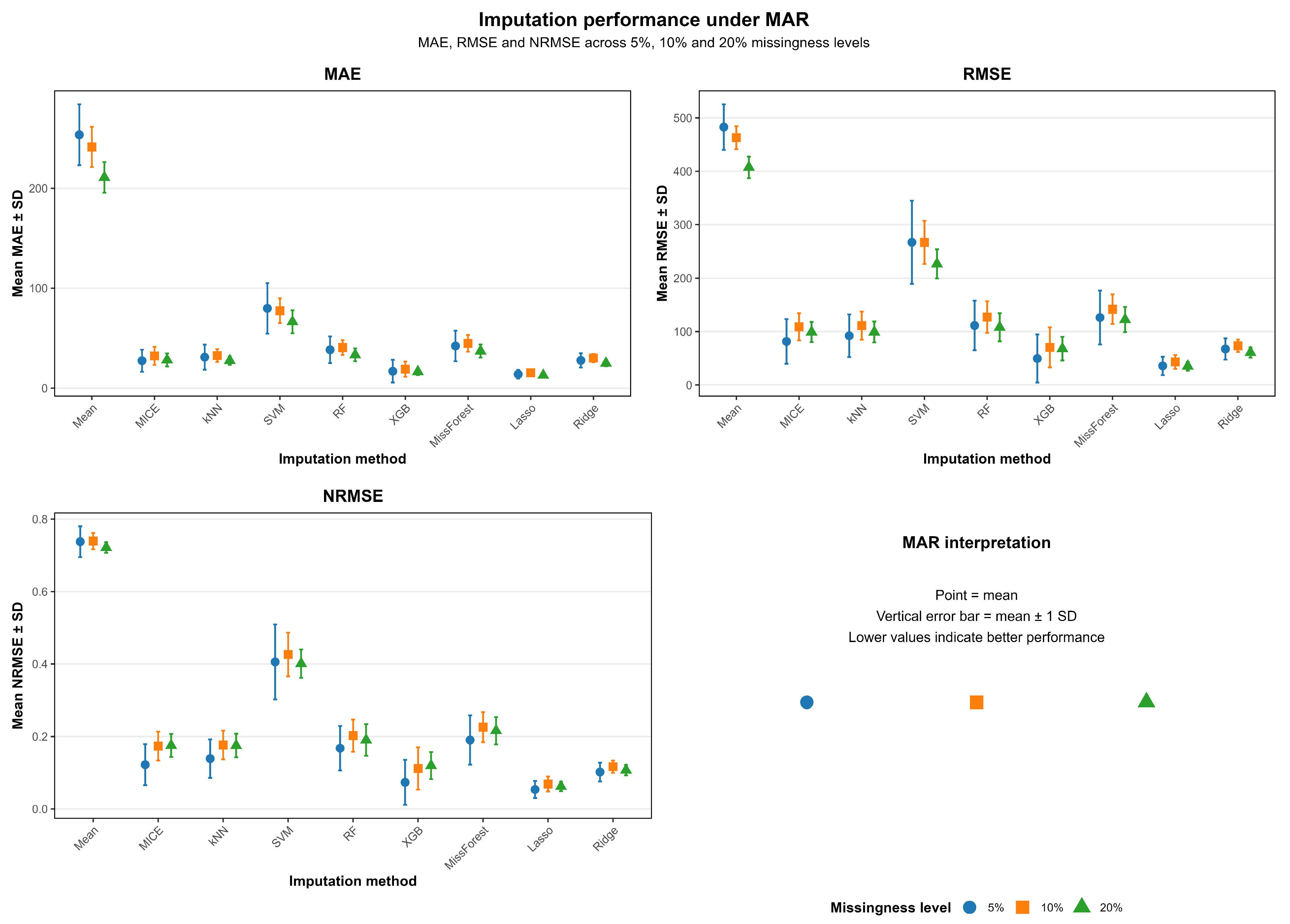
A different pattern was observed under the MAR mechanism, where imputation became considerably more challenging because missing values depended on observed variables. Overall prediction errors increased for all methods relative to MCAR, indicating the greater complexity introduced by systematic missingness. Nevertheless, Lasso consistently achieved the best overall performance, followed closely by XGB and Ridge, demonstrating their ability to exploit relationships among predictors when estimating missing values. Tree-based methods such as RF and MissForest provided moderate performance, whereas MICE and kNN were generally less accurate under this mechanism. Similar to the MCAR results, mean imputation remained the least effective approach, producing substantially larger errors across all evaluation metrics. Although increasing missingness generally led to reduced imputation accuracy, the relative ranking of the better-performing methods remained largely consistent, highlighting the robustness of regularized regression and gradient boosting approaches under MAR conditions. The imputation performance under MAR is given in Figure 3.

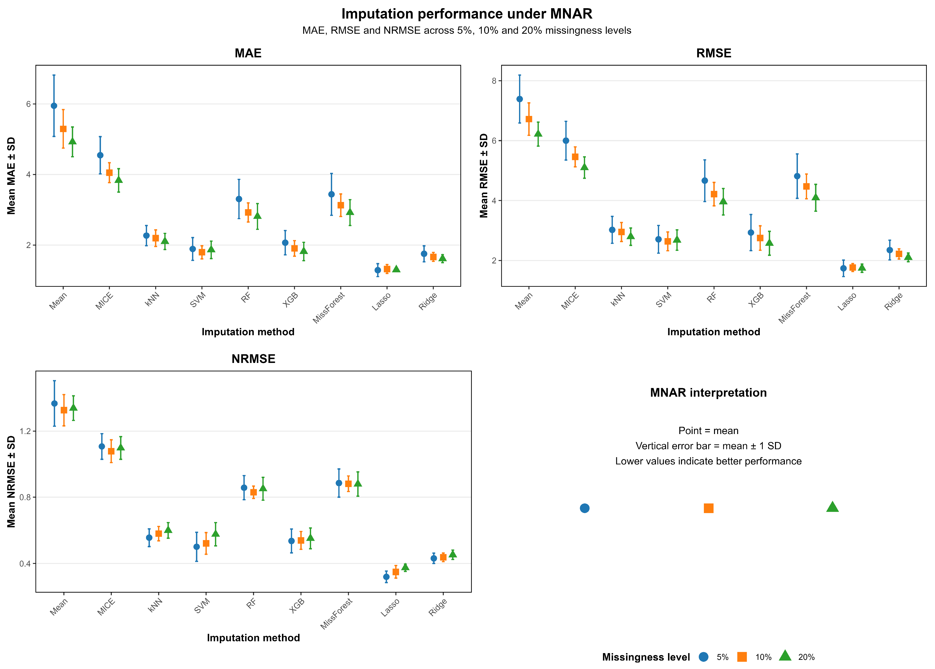
Under the MNAR mechanism, the overall magnitude of the imputation errors was considerably lower than under MAR, although differences between methods remained evident. Lasso consistently produced the most accurate imputations across all missingness levels, with Ridge frequently ranking second, while RF, MissForest, XGB, SVM, and kNN formed a middle-performing group with relatively similar performance. Unlike the MCAR and MAR scenarios, increasing the percentage of missingness had only a modest effect on the leading methods, indicating stable performance under the simulated MNAR mechanism. Mean imputation and MICE continued to exhibit comparatively poorer performance, particularly when evaluated using NRMSE, suggesting that these approaches were less capable of recovering the underlying data structure when missingness depended on the unobserved values themselves. Overall, the WDBC results indicate that regularized regression methods, particularly Lasso, provided the most reliable and consistent imputation performance across all missingness mechanisms and levels, whereas mean imputation consistently yielded the poorest results, reinforcing the advantages of model-based imputation techniques for breast cancer diagnostic data. The imputation performance under MNAR is given in Figure 4.

3.1.2. LBCC Dataset

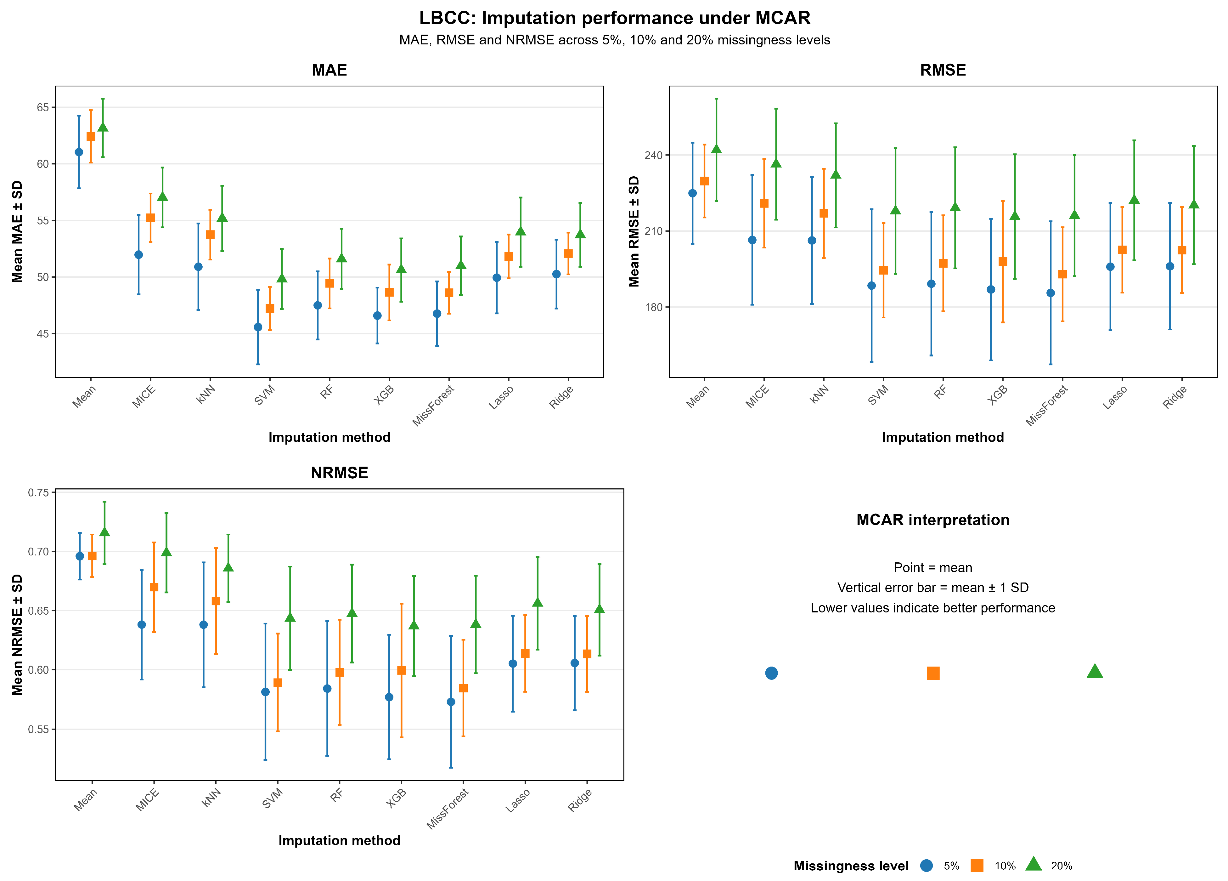
To evaluate the robustness of the imputation methods on the LBCC dataset, average imputation performance was compared across MCAR, MAR, and MNAR missingness mechanisms at 5%, 10%, and 20% missingness levels using MAE, RMSE, and NRMSE as performance metrics. Under the MCAR mechanism, MissForest and XGBoost (XGB) consistently produced the lowest reconstruction errors across the three missingness levels, with SVM also demonstrating highly competitive performance, particularly for MAE. Differences among these three methods were relatively small, indicating that they were robust when data were missing completely at random. Random Forest (RF) exhibited slightly higher errors but remained among the better-performing approaches. Lasso and Ridge achieved intermediate performance, whereas kNN and MICE generated comparatively larger reconstruction errors. As expected, Mean imputation consistently produced the highest MAE, RMSE, and NRMSE values, making it the least effective approach under MCAR. Increasing the missingness level from 5% to 20% resulted in only modest increases in prediction error for MissForest, XGB, SVM, and RF, whereas the degradation was more pronounced for Mean imputation, MICE, and kNN, demonstrating the greater robustness of the machine-learning-based methods to increasing levels of randomly missing data. The imputation performance under MCAR is given in Figure 5.

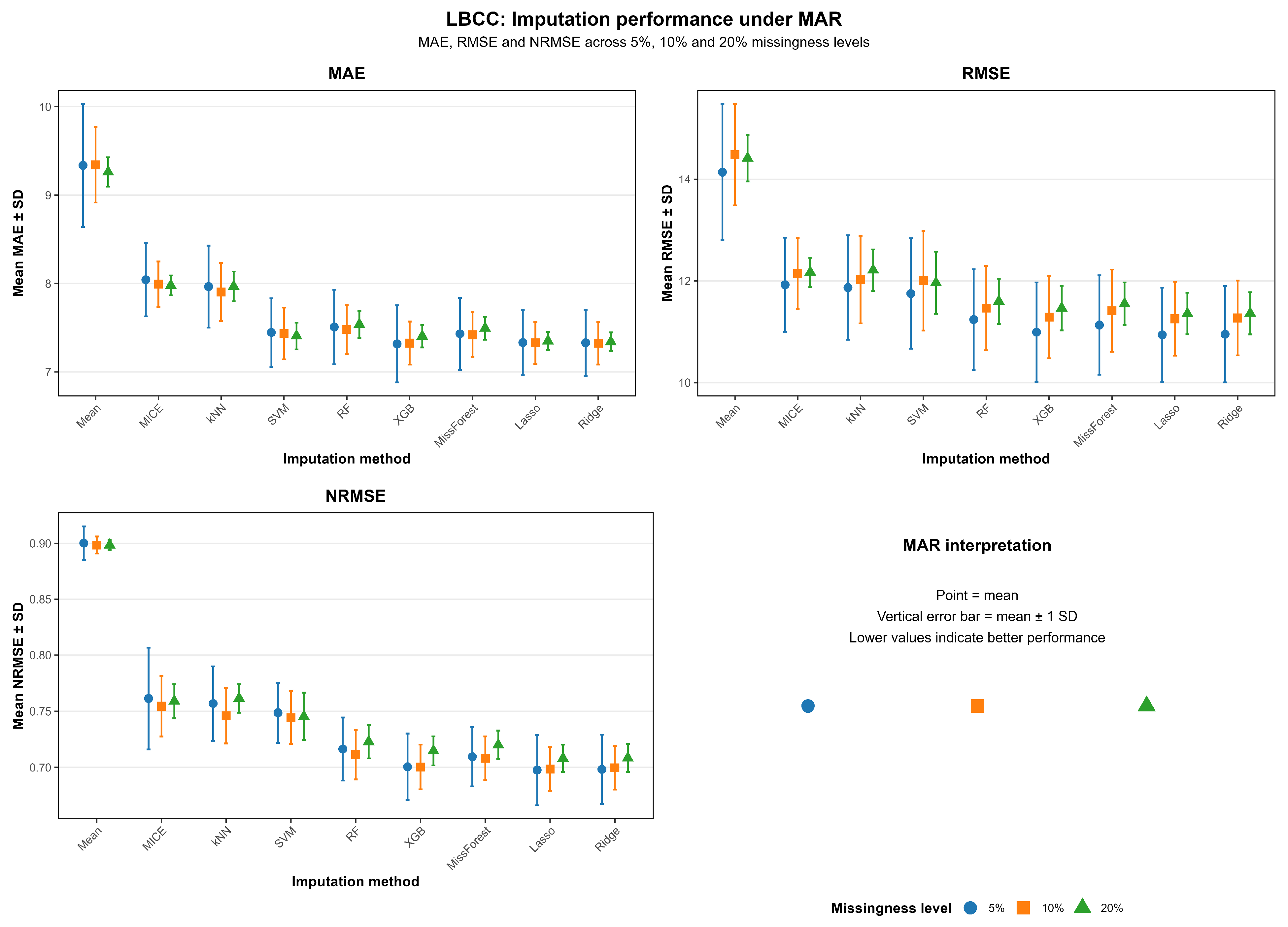
Under the MAR mechanism, Lasso consistently achieved the best overall imputation performance across all three missingness levels, recording the lowest RMSE and NRMSE while also maintaining one of the lowest MAE values. Ridge closely matched the performance of Lasso, with XGB ranking a very close third, indicating that these methods reconstructed missing values with comparable accuracy under missingness dependent on observed variables. MissForest and RF also performed well but with marginally higher reconstruction errors. Although SVM produced relatively low MAE values, its RMSE and NRMSE were consistently higher than those of the leading methods. MICE and kNN showed comparatively poorer performance, while Mean imputation again yielded the largest errors across all evaluation metrics. Notably, the performance of the leading methods remained remarkably stable as missingness increased from 5% to 20%, whereas larger increases in error were observed for Mean imputation, MICE, and kNN, particularly at the highest missingness level. The imputation performance under MAR is given in Figure 6.

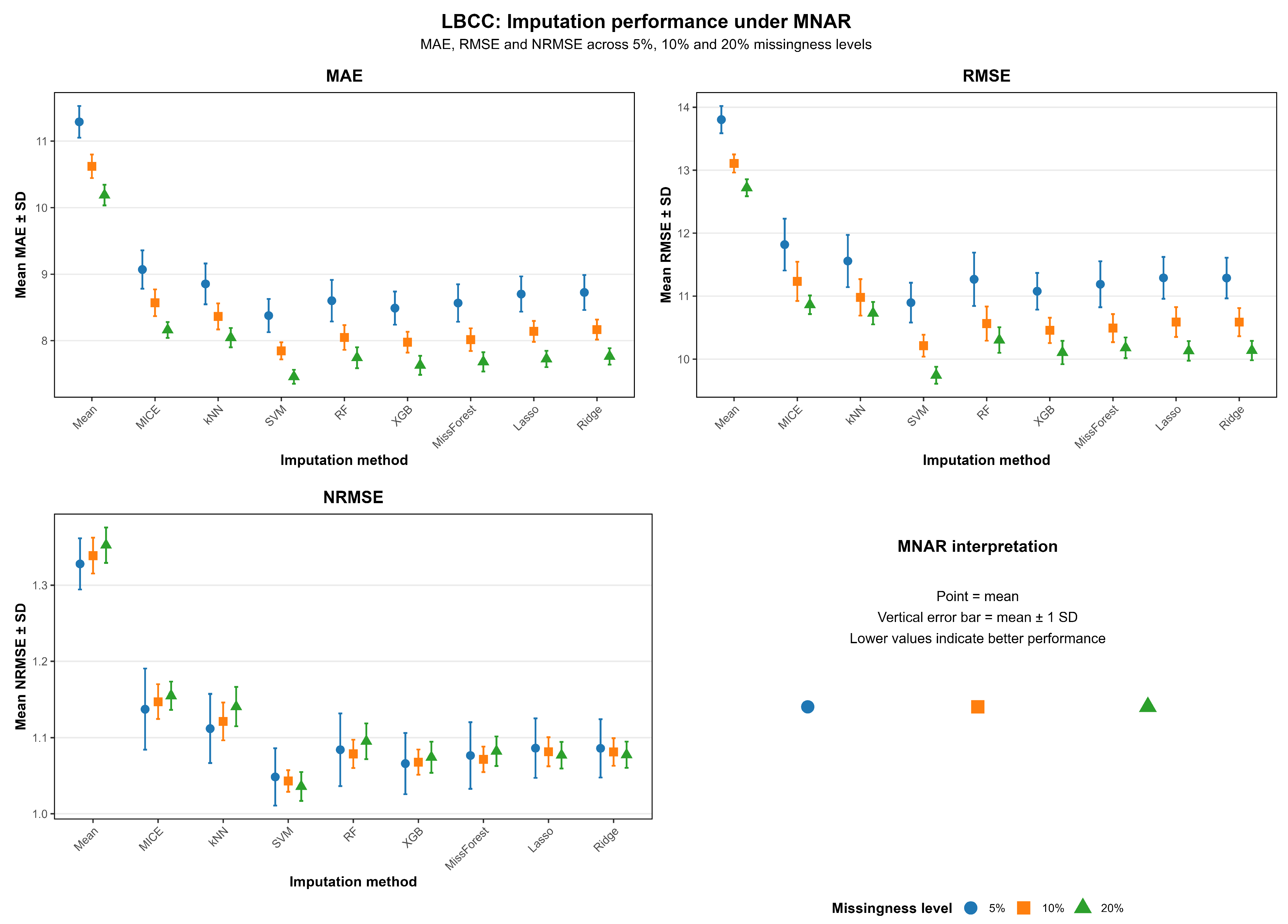
Under the MNAR mechanism, SVM emerged as the best-performing imputation method, consistently achieving the lowest MAE, RMSE, and NRMSE across all three missingness levels. XGB ranked second overall, followed closely by MissForest and RF, with only small differences separating these machine-learning approaches. Lasso and Ridge demonstrated similar intermediate performance, whereas MICE and kNN produced larger reconstruction errors. Mean imputation remained the poorest-performing approach, recording substantially higher errors than all other methods regardless of the evaluation metric. Interestingly, unlike the MCAR and MAR scenarios, prediction errors generally decreased slightly as the missingness level increased from 5% to 20%, although the relative ranking of the imputation methods remained largely unchanged. Overall, the results indicate that advanced machine-learning-based imputation methods, particularly SVM and XGB under MNAR, MissForest and XGB under MCAR, and Lasso under MAR, consistently provided more accurate and stable imputations than conventional approaches, while Mean imputation remained the least reliable across all missingness mechanisms. The imputation performance under MNAR is given in Figure 7.

Overall, the highest-performing methods exhibited relatively small variability across repeated simulations, indicating that their superior performance was not driven by a particular realization of the missing-data process. As expected, variability generally increased under the MNAR mechanism and at higher missingness levels, reflecting the greater uncertainty associated with more complex missing-data scenarios. These findings suggest that both average performance and variability should be considered when selecting imputation methods for breast cancer prediction.

3.2. Statistical Comparison of Imputation Methods

3.2.1. WDBC Dataset

The Friedman test was used to determine whether the nine imputation methods differed significantly in their reconstruction performance across the ten repeated missing-data simulations. Statistically significant differences were observed for MAE, RMSE and NRMSE under every combination of missingness mechanism and level, with all omnibus tests yielding $p<0.001$. The Friedman chi-square statistics ranged from 43.156 to 79.013, indicating substantial differences in the relative performance of the imputation methods across the WDBC experiments.

Kendall’s coefficient of concordance also indicated strong agreement in the rankings of the methods across the repeated simulations. The coefficient ranged from 0.790 to 0.988, with most values exceeding 0.90. The strongest agreement was observed for MAE under MNAR at 20% missingness ($W=0.988$), whereas the lowest agreement was recorded for RMSE and NRMSE under MCAR at 5% missingness ($W=0.790$). These large effect sizes demonstrate that the differences identified by the Friedman tests were not only statistically significant but were also associated with highly consistent performance rankings across the repeated datasets. The complete Friedman statistics and Kendall’s W effect sizes are provided in Appendix A (WDBC).

The overall average rankings further showed that Lasso was the best-performing imputation method, followed by XGB and Ridge (see

Table 4. Friedman test, Kendall’s coefficient of concordance and average ranks of the imputation methods for the WDBC dataset.

Panel A: Friedman Test Results
Missingness Scenario	Metric	Friedman ${\mathit{\chi }}^2$	df	p-Value	Kendall’s $\mathit{W}$
MCAR, 5%	MAE	75.147	8	<0.001	0.939
	RMSE	63.227	8	<0.001	0.790
	NRMSE	63.227	8	<0.001	0.790
MAR, 5%	MAE	75.840	8	<0.001	0.948
	RMSE	75.200	8	<0.001	0.940
	NRMSE	75.200	8	<0.001	0.940
MNAR, 5%	MAE	77.600	8	<0.001	0.970
	RMSE	77.893	8	<0.001	0.974
	NRMSE	77.893	8	<0.001	0.974
MCAR, 10%	MAE	78.213	8	<0.001	0.978
	RMSE	66.560	8	<0.001	0.832
	NRMSE	66.560	8	<0.001	0.832
MAR, 10%	MAE	75.813	8	<0.001	0.948
	RMSE	76.507	8	<0.001	0.956
	NRMSE	76.507	8	<0.001	0.956
MNAR, 10%	MAE	77.947	8	<0.001	0.974
	RMSE	77.467	8	<0.001	0.968
	NRMSE	77.467	8	<0.001	0.968
MCAR, 20%	MAE	47.156	8	<0.001	0.982
	RMSE	43.156	8	<0.001	0.899
	NRMSE	43.156	8	<0.001	0.899
MAR, 20%	MAE	74.720	8	<0.001	0.934
	RMSE	76.907	8	<0.001	0.961
	NRMSE	76.907	8	<0.001	0.961
MNAR, 20%	MAE	79.013	8	<0.001	0.988
	RMSE	77.893	8	<0.001	0.974
	NRMSE	77.893	8	<0.001	0.974
Panel B: Overall Average Ranking
Imputation Method			Average Rank
Lasso			1.465
XGB			2.535
Ridge			3.523
MICE			5.147
kNN			5.333
RF			5.423
SVM			6.279
MissForest			6.364
Mean			8.930

). Random Forest ranked fourth, while SVM, MICE and kNN occupied the middle positions. MissForest and Mean imputation were ranked eighth and ninth, respectively. This ranking is consistent with the descriptive findings, in which the regularised regression and gradient-boosting approaches generally produced lower reconstruction errors than the conventional Mean and distance-based methods.

Because the Friedman tests established significant overall differences, pairwise Wilcoxon signed-rank tests with Holm adjustment were conducted to identify the specific method pairs that differed. For MAE, 34 of the 36 pairwise comparisons were statistically significant. The only non-significant comparisons were MICE versus kNN ($p_{\mathrm{Holm}}=0.291$) and MICE versus RF ($p_{\mathrm{Holm}}=0.075$). Lasso significantly outperformed all other methods for MAE, including XGB ($p_{\mathrm{Holm}}=0.016$), while XGB also performed significantly better than Ridge, RF, MICE, MissForest, kNN, SVM and Mean imputation.

For RMSE, 33 of the 36 pairwise comparisons were significant. The differences between MICE and kNN ($p_{\mathrm{Holm}}=0.053$), kNN and RF ($p_{\mathrm{Holm}}=0.082$), and XGB and Ridge ($p_{\mathrm{Holm}}=0.082$) were not statistically significant. Lasso produced significantly lower RMSE values than all competing methods, including XGB ($p_{\mathrm{Holm}}=0.003$) and Ridge ($p_{\mathrm{Holm}}<0.001$).

For NRMSE, 29 of the 36 comparisons were significant. Non-significant differences were observed among several middle-performing methods, including MICE versus kNN, SVM, RF and MissForest; SVM versus RF and MissForest; and XGB versus Ridge (See

Table 5. Summary of pairwise Wilcoxon signed-rank comparisons with Holm correction for the WDBC dataset.

Metric	Total Comparisons	Significant Comparisons	Non-Significant Comparisons
MAE	36	34	MICE–kNN; MICE–RF
RMSE	36	33	MICE–kNN; kNN–RF; XGB–Ridge
NRMSE	36	29	MICE–kNN; MICE–SVM; MICE–RF; MICE–MissForest; SVM–RF; SVM–MissForest; XGB–Ridge

Note: Holm-adjusted p < 0.05 was considered statistically significant. The complete pairwise test statistics are presented in the Appendix A.

). Nevertheless, Lasso remained significantly better than every other method, while XGB and Ridge generally outperformed the lower-ranked approaches. Mean imputation was significantly inferior to all eight competing methods across MAE, RMSE and NRMSE.

3.2.2. LBCC Dataset

The Friedman test was used to determine whether the nine imputation methods differed significantly in their reconstruction performance across the repeated missing-data simulations for the LBCC dataset. Statistically significant differences were observed for MAE, RMSE and NRMSE under every combination of missingness mechanism and missingness level, with all omnibus tests yielding p < 0.001. The Friedman chi-square statistics ranged from 61.467 to 77.093, indicating substantial differences in the relative performance of the imputation methods across the LBCC experiments.

Kendall’s coefficient of concordance likewise demonstrated strong agreement in the rankings of the methods across the repeated simulations. The coefficient ranged from 0.768 to 0.964, with most values exceeding 0.85, indicating large effect sizes and highly consistent rankings of the competing imputation methods. The strongest agreement was observed for MAE under MNAR at 10% missingness (W = 0.964), whereas the lowest agreement occurred for RMSE and NRMSE under MCAR at 5% missingness (W = 0.768). These findings demonstrate that the statistically significant differences identified by the Friedman tests were accompanied by highly reproducible performance rankings across repeated simulations, despite the larger sample size and greater heterogeneity of the LBCC dataset.

The overall average rankings further showed that XGB was the best-performing imputation method, followed by SVM and MissForest. Lasso and Ridge ranked fourth and fifth, respectively, while Random Forest occupied the sixth position (

Table 6. Friedman test, Kendall’s coefficient of concordance (W), and average ranks of the imputation methods for the LBCC dataset.

Panel A: Friedman Test Results
Missingness Scenario	Metric	Friedman χ2	df	p-Value	Kendall’s W
MCAR, 5%	MAE	69.893	8	<0.001	0.874
	RMSE	61.467	8	<0.001	0.768
	NRMSE	61.467	8	<0.001	0.768
MAR, 5%	MAE	67.440	8	<0.001	0.843
	RMSE	67.440	8	<0.001	0.843
	NRMSE	67.440	8	<0.001	0.843
MNAR, 5%	MAE	74.027	8	<0.001	0.925
	RMSE	73.333	8	<0.001	0.917
	NRMSE	73.333	8	<0.001	0.917
MCAR, 10%	MAE	76.960	8	<0.001	0.962
	RMSE	66.560	8	<0.001	0.832
	NRMSE	66.560	8	<0.001	0.832
MAR, 10%	MAE	66.560	8	<0.001	0.832
	RMSE	68.560	8	<0.001	0.857
	NRMSE	68.560	8	<0.001	0.857
MNAR, 10%	MAE	77.093	8	<0.001	0.964
	RMSE	71.413	8	<0.001	0.893
	NRMSE	71.413	8	<0.001	0.893
MCAR, 20%	MAE	75.760	8	<0.001	0.947
	RMSE	69.600	8	<0.001	0.870
	NRMSE	69.600	8	<0.001	0.870
MAR, 20%	MAE	72.000	8	<0.001	0.900
	RMSE	72.160	8	<0.001	0.902
	NRMSE	72.160	8	<0.001	0.902
MNAR, 20%	MAE	76.480	8	<0.001	0.956
	RMSE	75.653	8	<0.001	0.946
	NRMSE	75.653	8	<0.001	0.946
Panel B: Overall Average Ranking
Imputation Method			Average Rank
XGB			2.474
SVM			3.067
MissForest			3.193
Lasso			3.933
Ridge			4.156
RF			4.504
kNN			7.085
MICE			7.641
Mean			8.948

). kNN and MICE ranked seventh and eighth, whereas Mean imputation consistently ranked last. Compared with the WDBC dataset, where Lasso achieved the highest overall ranking, the LBCC dataset favoured ensemble machine-learning approaches, particularly gradient boosting and kernel-based learning. This shift suggests that flexible nonlinear models are better able to capture the greater variability and more complex relationships present in large longitudinal epidemiological datasets. Nevertheless, the consistently poor ranking of Mean imputation across both datasets reinforces the limitations of simple deterministic imputation methods for breast cancer research. The complete Friedman statistics and Kendall’s W effect sizes are provided in Appendix B (LBCC).

Because the Friedman tests established significant overall differences, pairwise Wilcoxon signed-rank tests with Holm adjustment were conducted to identify the specific method pairs that differed. Under MCAR, 34 of the 36 pairwise comparisons were statistically significant for MAE, while 29 comparisons were significant for both RMSE and NRMSE. Under MAR, 31 of the 36 comparisons were statistically significant for each of the three performance metrics. The greatest separation among methods was observed under MNAR, where all 36 pairwise comparisons were statistically significant for MAE, while 31 comparisons remained significant for RMSE and NRMSE.

The pairwise analyses largely corroborated the Friedman rankings. Under MCAR, the only non-significant MAE comparisons were between Lasso and Ridge and between MissForest and XGB, suggesting comparable reconstruction performance among these leading methods. For RMSE and NRMSE, most non-significant comparisons involved neighbouring machine-learning methods, including MissForest, SVM, RF and XGB, whereas MICE and kNN also showed similar performance. Under MAR, the non-significant comparisons primarily occurred among the higher-ranked methods (Lasso, Ridge and XGB) and between MICE, kNN and SVM, indicating relatively small performance differences within these groups. Under MNAR, all MAE comparisons were statistically significant, demonstrating complete discrimination among the competing methods (see

Table 7. Summary of pairwise Wilcoxon signed-rank comparisons with Holm correction for the LBCC dataset.

Mechanism	Metric	Total Comparisons	Significant Comparisons	Non-Significant Comparisons
MCAR	MAE	36	34	Lasso–Ridge; MissForest–XGB
	RMSE	36	29	Lasso–Ridge; MICE–kNN; MissForest–SVM; MissForest–XGB; RF–SVM; RF–XGB; SVM–XGB
	NRMSE	36	29	Lasso–Ridge; MICE–kNN; MissForest–SVM; MissForest–XGB; RF–SVM; RF–XGB; SVM–XGB
MAR	MAE	36	31	Lasso–Ridge; Lasso–XGB; Ridge–XGB; MICE–kNN; MissForest–SVM
	RMSE	36	31	Lasso–XGB; Ridge–XGB; MICE–kNN; MICE–SVM; SVM–kNN
	NRMSE	36	31	Lasso–XGB; Ridge–XGB; MICE–kNN; MICE–SVM; SVM–kNN
MNAR	MAE	36	36	None
	RMSE	36	31	Lasso–MissForest; Lasso–RF; Lasso–Ridge; MissForest–Ridge; RF–Ridge
	NRMSE	36	31	Lasso–MissForest; Lasso–RF; Lasso–Ridge; MissForest–Ridge; RF–Ridge

Note: Holm-adjusted p < 0.05 was considered statistically significant. The complete pairwise Wilcoxon signed-rank test statistics, adjusted p-values and effect sizes are presented in the Appendix B because the full analysis comprises 324 pairwise comparisons across the three missingness mechanisms, three missingness levels and three evaluation metrics.

). In contrast, the few non-significant RMSE and NRMSE comparisons were confined to Lasso, Ridge, Random Forest and MissForest, again indicating that differences among the best-performing methods were comparatively modest. Overall, Mean imputation remained significantly inferior to the advanced machine-learning approaches across virtually all comparisons, providing further evidence that sophisticated imputation techniques offer substantially more reliable reconstruction of incomplete longitudinal breast cancer data. Detailed pairwise comparisons for the WDBC and LBCC datasets are provided in Appendix C and Appendix D, respectively.

3.3. Classification Performance

3.3.1. WDBC Dataset

To assess the effect of missing data and imputation on diagnostic performance, the classification results obtained after imputation were compared with the baseline models trained on the complete WDBC dataset. Before introducing missing values, LightGBM achieved the highest classification performance, with an accuracy of 0.9912, perfect specificity (1.000), perfect precision (1.000) and a Kappa coefficient of 0.981. Random Forest ranked second with an accuracy of 0.9823 and Kappa of 0.9621, while Logistic Regression achieved an accuracy of 0.9469 and Kappa of 0.8863 (

Table 8. Classification performance of the baseline models and the best imputation–classifier combinations for the WDBC dataset.

Panel A. Baseline Classification Performance (Complete Dataset)
Model		Accuracy	Sensitivity		Specificity		Precision		Kappa
Logistic Regression		0.9469	0.9286		0.9577		0.9286		0.8863
Random Forest		0.9823	0.9762		0.9859		0.9762		0.9621
LightGBM		0.9912	0.9762		1.0000		1.0000		0.9810
Panel B. Best Imputation–Classifier Combinations
Mechanism	Missingness	Best Imputation	Best Classifier	Accuracy		Sensitivity	Specificity	Precision		Kappa
MCAR	5%	Lasso	LightGBM	0.9626		0.9374	0.9776	0.9622		0.9196
MCAR	10%	XGB	LightGBM	0.9614		0.9436	0.9720	0.9523		0.9171
MCAR	20%	XGB	LightGBM	0.9579		0.9342	0.9720	0.9516		0.9094
MAR	5%	Lasso	LightGBM	0.9635		0.9378	0.9787	0.9639		0.9214
MAR	10%	Lasso	LightGBM	0.9624		0.9336	0.9796	0.9652		0.9190
MAR	20%	Lasso	LightGBM	0.9647		0.9416	0.9784	0.9637		0.9241
MNAR	5%	Lasso	RF	0.9596		0.9386	0.9720	0.9537		0.9133
MNAR	10%	Lasso	LightGBM	0.9649		0.9411	0.9790	0.9646		0.9245
MNAR	20%	Lasso	RF	0.9613		0.9434	0.9720	0.9540		0.9171

). Following missingness creation and imputation, LightGBM remained the best-performing classifier in seven of the nine missing-data scenarios, whereas Random Forest performed best under MNAR at 5% and 20% missingness. Lasso was the preferred imputation method in seven scenarios, while XGB was selected under MCAR at 10% and 20% missingness.

Compared with the baseline models, classification performance declined only modestly after missingness creation and imputation. The highest post-imputation accuracy was 0.9649 under MNAR at 10% missingness using Lasso imputation and LightGBM classification, representing a reduction of 2.64 percentage points from the LightGBM baseline accuracy of 0.9912. Similarly, the highest post-imputation Kappa coefficient (0.9245) remained close to the baseline value of 0.9810, indicating that substantial agreement was preserved despite the introduction of missing data. Sensitivity after imputation ranged from 0.9336 to 0.9436, compared with the baseline value of 0.9762 for both Random Forest and LightGBM. Specificity ranged from 0.9720 to 0.9796, remaining close to the baseline values of 0.9859 for Random Forest and 1.0000 for LightGBM. Precision also remained consistently high (0.9516–0.9652), although slightly below the perfect precision achieved by the baseline LightGBM model. Overall, the results demonstrate that the proposed imputation framework preserved a high level of diagnostic performance across all missingness mechanisms and levels. Although some reduction relative to the complete-data baseline was observed, the decline was small, indicating that Lasso and XGB imputation effectively mitigated the adverse effects of missing data, particularly when combined with the LightGBM classifier. Complete classification results for all evaluated imputation method–classifier combinations are presented in Appendix E.

3.3.2. LBCC Dataset

To evaluate the effects of missing data, imputation, and class balancing on breast cancer classification, the performance of the imputed datasets was compared with baseline models trained on the complete LBCC dataset without imputation or Borderline-SMOTE. Before introducing missing values and applying class balancing, all three classifiers (Logistic Regression, Random Forest, and LightGBM) produced near-identical results, achieving an accuracy of 0.9956 and perfect specificity (1.000), but failed to identify any breast cancer cases, resulting in zero sensitivity and a Kappa coefficient of zero (

Table 9. Classification performance of the baseline models and the best imputation–classifier combinations for the LBCC dataset.

Panel A. Baseline Classification Performance (Complete Dataset)
Model		Accuracy	Sensitivity		Specificity		Precision		Kappa
Logistic Regression		0.9956	0.0000		1.0000		NA		0.0000
Random Forest		0.9956	0.0000		1.0000		NA		0.0000
LightGBM		0.9956	0.0000		1.0000		NA		0.0000
Panel B. Best Imputation–Classifier Combinations
Mechanism	Missingness	Best Imputation	Best Classifier	Accuracy		Sensitivity	Specificity	Precision		Kappa
MCAR	5%	SVM	RF	0.9805		0.1124	0.9933	0.2032		0.1350
MCAR	10%	SVM	RF	0.9831		0.0562	0.9967	0.1738		0.0772
MCAR	20%	Mean	RF	0.9825		0.0571	0.9961	0.2000		0.0790
MAR	5%	XGB	RF	0.9799		0.0971	0.9929	0.1743		0.1147
MAR	10%	SVM	RF	0.9799		0.1390	0.9922	0.2094		0.1549
MAR	20%	kNN	RF	0.9801		0.1676	0.9920	0.2356		0.1850
MNAR	5%	RF	RF	0.9795		0.1248	0.9920	0.1667		0.1310
MNAR	10%	SVM	RF	0.9807		0.1533	0.9929	0.2371		0.1765
MNAR	20%	Mean	RF	0.9809		0.1676	0.9929	0.2198		0.1787

). Precision was undefined because no positive cases were predicted. These findings reflect the severe class imbalance in the LBCC dataset, where the overwhelming majority of observations belonged to the non-cancer class.

Following missingness creation, imputation, and application of BSMOTE during model training, classification performance improved substantially with respect to minority-class detection. Random Forest consistently emerged as the best-performing classifier across all nine missingness scenarios, while the optimal imputation method varied according to the missingness mechanism and level. SVM imputation was selected most frequently, producing the highest-performing Random Forest models under MCAR at 5% and 10% missingness, MAR at 10% missingness, and MNAR at 10% missingness. Mean imputation was preferred under MCAR at 20% and MNAR at 20%, whereas XGB, kNN, and Random Forest imputation each produced the best-performing model in one missingness scenario.

Compared with the baseline models, overall classification accuracy decreased modestly from 0.9956 to 0.9795–0.9831 following missingness creation, imputation, and BSMOTE. However, this reduction in accuracy was accompanied by a marked improvement in the model’s ability to identify breast cancer cases. Whereas the baseline models failed to detect any positive cases (sensitivity = 0.000 and Kappa = 0.000), the imputed and balanced models achieved sensitivities ranging from 0.0562 to 0.1676 and Kappa coefficients between 0.0772 and 0.1850. Specificity remained consistently high (0.9920–0.9967), indicating that the improvement in minority-class detection was achieved with only a minimal increase in false-positive classifications. Precision also increased from an undefined value at baseline to 0.1667–0.2371 across the best-performing models.

Overall, the results demonstrate that although the use of imputation and BSMOTE resulted in a slight reduction in overall accuracy, they substantially improved the clinical usefulness of the classification models by enabling the detection of breast cancer cases that were entirely missed by the baseline classifiers. Among the evaluated approaches, Random Forest consistently provided the most robust classification performance, while the optimal imputation method depended on the missingness mechanism and level. Complete classification results for all evaluated imputation method–classifier combinations are presented in Appendix F.

4. Discussion

This study systematically evaluated nine statistical and machine learning-based imputation methods under three missing-data mechanisms (MCAR, MAR and MNAR) using two publicly available breast cancer datasets representing complementary clinical settings. Unlike many previous studies that evaluate imputation methods solely on reconstruction accuracy, this study simultaneously assessed their impact on downstream breast cancer classification within a repeated nested cross-validation framework. The findings demonstrate that the performance of imputation methods depended on both the characteristics of the dataset and the missing-data mechanism. Across both datasets, advanced machine learning and regularized regression methods generally achieved lower reconstruction errors than conventional deterministic approaches, although the optimal imputation method differed between datasets. These findings support recent evidence that no single imputation method is universally optimal and that method performance should be evaluated within the context of the data structure, missingness mechanism and intended downstream analytical task [16,17].

A notable finding was the contrasting behaviour of the evaluated methods across the two study datasets. For the WDBC dataset, Lasso consistently achieved the best overall reconstruction performance, followed by XGBoost and Ridge. In contrast, XGBoost ranked first for the LBCC dataset, with SVM and MissForest also demonstrating competitive performance. This difference is consistent with the distinct characteristics of the two datasets. The WDBC dataset comprises highly correlated continuous morphometric features extracted from digitised breast cell images, whereas the LBCC dataset contains heterogeneous demographic, anthropometric, lifestyle and biochemical variables collected from a longitudinal cohort. Regularized regression methods such as Lasso are particularly effective when predictors exhibit substantial correlation because coefficient shrinkage reduces estimation variance while simultaneously selecting informative variables [18,19]. Conversely, gradient boosting methods such as XGBoost are capable of modelling nonlinear relationships and complex interactions without requiring explicit model specification [17]. The present findings therefore suggest that the observed differences between datasets are more likely to reflect differences in predictor structure than inherent superiority of one imputation algorithm over another. Similar conclusions have been reached in recent comparative reviews, which emphasize that the relative performance of imputation methods depends strongly on data characteristics rather than on algorithm class alone [20].

The influence of the missing-data mechanism was evident throughout the study. Under MCAR, where missingness was generated independently of the observed and unobserved data, several advanced imputation methods produced relatively similar reconstruction accuracy, particularly at lower levels of missingness. This behaviour is expected because MCAR does not introduce systematic bias into the estimation process and therefore represents the least challenging missing-data scenario [5]. Nevertheless, Mean imputation consistently produced substantially larger reconstruction errors than all model-based approaches across both datasets. Although computationally simple, Mean imputation ignores multivariate relationships among predictors and reduces data variability, which can distort covariance structures and attenuate associations between variables [16]. The consistently poor performance of Mean imputation observed in this study therefore reinforces longstanding recommendations that deterministic single-value substitution should be avoided when more informative model-based alternatives are available.

Performance differences became more pronounced under MAR, where missingness depended on observed variables. For the WDBC dataset, Lasso maintained the highest overall performance, while XGBoost, Ridge and MissForest also produced comparatively low reconstruction errors. In the LBCC dataset, Lasso, Ridge and XGBoost formed a group of similarly high-performing methods. These findings are broadly consistent with the theoretical assumptions underlying MAR, under which observed predictors contain information that can be exploited to estimate missing values [15]. Regularized regression methods benefit from stable estimation when predictor correlation is high, whereas ensemble learning methods exploit nonlinear dependencies and interaction effects among predictors. Interestingly, MICE did not consistently rank among the strongest methods despite its widespread recommendation for MAR data. This does not contradict the theoretical validity of multiple imputation under MAR but rather reflects that predictive performance depends on model specification and the complexity of the underlying relationships. Previous methodological studies have similarly reported that MICE may be less competitive than machine learning approaches when predictor interactions are highly nonlinear or when data contain heterogeneous feature distributions [9,20].

The simulated MNAR scenarios represented the most challenging conditions because missingness depended directly on the values being imputed. Although advanced methods continued to outperform simpler approaches, the leading algorithms differed between datasets. Lasso remained the best-performing method for the WDBC dataset, whereas SVM and XGBoost achieved the lowest reconstruction errors for the LBCC dataset. These findings should be interpreted carefully. The present study simulated MNAR using predefined logistic mechanisms to create controlled experimental conditions rather than reproducing naturally occurring clinical missingness. Consequently, the results demonstrate comparative robustness under the specified simulation framework rather than establishing that these methods are universally superior under MNAR conditions. This distinction is important because MNAR mechanisms are inherently untestable from the observed data alone, and no general-purpose imputation method can guarantee unbiased estimation without additional assumptions regarding the missing-data process [5]. Nevertheless, the results suggest that flexible nonlinear learning algorithms and regularized regression methods may retain greater predictive capability than deterministic approaches when missingness departs from the standard MAR assumption.

The statistical analyses provide further support for these observations. Across both datasets, Friedman tests identified statistically significant differences among the nine imputation methods under every missing-data mechanism and missingness level, while Kendall’s coefficients of concordance indicated strong agreement in the rankings across repeated simulation runs. Moreover, the pairwise Wilcoxon signed-rank tests showed that many of the observed differences remained statistically significant after Holm correction, particularly when comparing the highest-ranked methods with Mean imputation. However, several comparisons among the leading machine learning methods were not statistically significant, particularly under MCAR and MAR for the LBCC dataset. These findings indicate that although advanced methods generally outperformed simpler approaches, differences among the best-performing algorithms were often relatively modest. Consequently, practical considerations such as computational efficiency, implementation complexity and model interpretability may influence method selection when reconstruction performance is comparable. This observation is consistent with recent recommendations advocating evidence-based selection of imputation methods rather than assuming the universal superiority of any single algorithm [9,20].

An important contribution of the present study is the simultaneous evaluation of imputation accuracy and downstream classification performance. Many comparative imputation studies conclude after reporting reconstruction error, implicitly assuming that more accurate imputations necessarily produce better predictive models. The results of this study demonstrate that the relationship is more nuanced. For the WDBC dataset, LightGBM achieved the highest classification performance using the complete data and remained the best-performing classifier in seven of the nine missing-data scenarios following imputation, while Random Forest achieved the highest performance in the remaining two MNAR scenarios. Although modest reductions in classification accuracy, sensitivity and Cohen’s Kappa were observed after introducing missingness, the decreases were relatively small, indicating that the best-performing imputation methods preserved much of the predictive information contained within the complete data. These findings suggest that reconstruction accuracy provides a useful, although incomplete, indicator of downstream predictive performance.

The LBCC dataset illustrates this distinction even more clearly. Before class balancing, all baseline classifiers achieved very high overall accuracy but failed to identify any breast cancer cases, resulting in zero sensitivity and a Cohen’s Kappa coefficient of zero. This outcome reflects the severe class imbalance present in the cohort rather than poor model implementation. Following imputation and application of Borderline-SMOTE within the training folds, Random Forest consistently achieved the highest classification performance across all missing-data scenarios. The improvement in sensitivity and Kappa demonstrates that evaluation based solely on overall accuracy would have produced misleading conclusions regarding classifier effectiveness. Consequently, the present findings reinforce the importance of assessing downstream predictive performance using multiple complementary metrics, particularly when analysing imbalanced clinical datasets where accurate identification of minority cases is of primary clinical interest. Similar recommendations have been made in recent machine learning studies emphasising that reconstruction accuracy alone is insufficient for selecting imputation strategies intended for predictive modelling [21,22].

This study possesses several methodological strengths. Two complementary breast cancer datasets representing diagnostic and longitudinal epidemiological settings were analysed using a common experimental framework. Artificial missingness was generated under three distinct mechanisms and multiple missingness levels, enabling systematic comparison of imputation performance under controlled conditions. The evaluation combined reconstruction error metrics with downstream classification, while repeated simulation and nested cross-validation reduced the likelihood of optimistic performance estimates arising from information leakage. Together, these design features provide a comprehensive assessment of imputation performance under conditions relevant to biomedical prediction studies.

The study also has limitations that should be considered when interpreting the findings. First, the missing-data mechanisms were simulated rather than observed and therefore cannot fully capture the complexity of missingness encountered in routine clinical practice. Second, although two datasets with contrasting characteristics were analysed, the findings should not be extrapolated to all breast cancer datasets or other biomedical domains without additional validation. Finally, only three classification algorithms were evaluated. Future research should investigate whether the observed performance patterns remain consistent across additional clinical datasets, alternative machine learning algorithms and naturally occurring missing-data scenarios.

Overall, the present study contributes to the methodological literature on missing-data handling by demonstrating that rigorous evaluation should extend beyond reconstruction error to include downstream predictive performance. Rather than identifying a universally superior imputation method, the findings indicate that method selection should be informed by dataset characteristics, the assumed missing-data mechanism and the objectives of the subsequent predictive analysis. This evidence supports a more context-specific approach to imputation method selection in breast cancer prediction studies, while highlighting the importance of validating imputation strategies within the analytical framework for which they are intended.

5. Conclusions

This study systematically compared nine statistical and machine learning-based imputation methods under simulated MCAR, MAR and MNAR missing-data mechanisms using two breast cancer datasets with distinct characteristics. By combining reconstruction accuracy with downstream classification performance within a repeated nested cross-validation framework, the study provides a comprehensive evaluation of imputation methods that extends beyond the conventional assessment based solely on reconstruction error. This dual evaluation framework offers a more complete assessment of the practical implications of missing-data handling for predictive modelling in breast cancer research.

The results demonstrated that no single imputation method consistently achieved the best performance across both datasets. For the WDBC dataset, Lasso produced the most accurate overall reconstruction, followed by XGBoost and Ridge, whereas XGBoost ranked highest for the LBCC dataset, with SVM and MissForest also demonstrating competitive performance. These findings indicate that imputation performance depends on the interaction between the characteristics of the dataset and the underlying missing-data mechanism rather than the choice of algorithm alone. Conventional Mean imputation consistently yielded the poorest reconstruction accuracy across both datasets, reinforcing previous recommendations that deterministic single-value substitution should be avoided when more informative model-based alternatives are available.

Evaluation of downstream classification further demonstrated that effective imputation can preserve predictive performance despite the presence of missing data. LightGBM remained the best-performing classifier for most WDBC scenarios, while Random Forest consistently achieved the highest classification performance for the LBCC dataset following imputation and class balancing. Importantly, the study showed that reconstruction accuracy alone is insufficient for selecting imputation methods intended for predictive modelling, as methods producing similar reconstruction errors may differ in their ability to preserve clinically relevant classification performance.

The findings should be interpreted within the scope of the experimental design. The missing-data mechanisms were generated through simulation, and the evaluated datasets represent only two breast cancer populations with distinct predictor characteristics. Consequently, the results should not be interpreted as establishing a universally optimal imputation method. Instead, they provide empirical evidence that imputation method selection should be guided by dataset characteristics, assumptions regarding the missing-data mechanism and the intended downstream analytical objective. Future studies should extend this evaluation to additional clinical datasets with naturally occurring missingness, investigate emerging deep learning-based imputation approaches, and examine the generalisability of these findings across other biomedical prediction tasks.

References

1. World Health Organization. Breast Cancer. Available online: https://www.who.int/news-room/fact-sheets/detail/breast-cancer (accessed on 9 June 2026).
2. Kallah-Dagadu, G.; Mohammed, M.; Nasejje, J.B.; Mchunu, N.N.; Twabi, H.S.; Batidzirai, J.M.; Singini, G.C.; Nevhungoni, P.; Maposa, I. Breast Cancer Prediction Based on Gene Expression Data Using Interpretable Machine Learning Techniques. Sci. Rep. 2025, 15, 7594. [Google Scholar] [CrossRef] [Scilit] [PubMed]
3. Akter, S.; Adesola, R.O.; Basnet, S. Machine Learning Approach to Identify Significant Genes and Classify Cancer Types from RNA-Seq Data. Glob. Med. Genet. 2025, 12, 100079. [Google Scholar] [CrossRef] [Scilit] [PubMed]
4. Azur, M.J.; Stuart, E.A.; Frangakis, C.; Leaf, P.J. Multiple Imputation by Chained Equations: What Is It and How Does It Work? Int. J. Methods Psychiatr. Res. 2011, 20, 40–49. [Google Scholar] [CrossRef] [Scilit] [PubMed]
5. Little, R.J.; Rubin, D.B. Statistical Analysis with Missing Data, 3rd ed.; Wiley Series in Probability and Statistics; Wiley: Hoboken, NJ, USA, 2019; Available online: https://onlinelibrary.wiley.com/doi/book/10.1002/9781119482260 (accessed on 9 June 2026).
6. Nyakundi, G.N.; Ndiritu, J.; Mwaniki Ivivi, J.; Kamanu, T. Class Prediction of High-Dimensional Data with Class Imbalance: Breast Cancer Gene Expression Data. Int. J. Adv. Sci. Res. Eng. 2024, 10, 28–46. [Google Scholar] [CrossRef] [Scilit]
7. Nyakundi, G.; Ndiritu, J.; Mwaniki, J.; Kamanu, T. Leveraging on hybrid machine learning models for early breast cancer detection. JP J. Biostat. 2026, 26, 11–40. [Google Scholar] [CrossRef] [Scilit]
8. Nyakundi, G.; Ndiritu, J.; Mwaniki, J.; Kamanu, T. Machine Learning for Breast Cancer Diagnosis: A Review of High-Dimensional and Class-Imbalanced Data Approaches. J. Agric. Sci. Technol. 2026, 25, 1–27. [Google Scholar] [CrossRef] [Scilit]
9. Stekhoven, D.J.; Bühlmann, P. MissForest—Non-Parametric Missing Value Imputation for Mixed-Type Data. Bioinformatics 2012, 28, 112–118. [Google Scholar] [CrossRef] [Scilit] [PubMed]
10. Jerez, J.M.; Molina, I.; García-Laencina, P.J.; Alba, E.; Ribelles, N.; Martín, M.; Franco, L. Missing Data Imputation Using Statistical and Machine Learning Methods in a Real Breast Cancer Problem. Artif. Intell. Med. 2010, 50, 105–115. [Google Scholar] [CrossRef] [Scilit] [PubMed]
11. Fan, J.; Lv, J. A Selective Overview of Variable Selection in High Dimensional Feature Space. Stat. Sin. 2010, 20, 101–148. [Google Scholar] [PubMed]
12. Li, H.; Ding, M.; Zhang, R.; Xiu, C. Motor Imagery EEG Classification Algorithm Based on CNN-LSTM Feature Fusion Network. Biomed. Signal Process. Control 2022, 72, 103342. [Google Scholar] [CrossRef] [Scilit]
13. Wolberg, W.H.; Street, W.N.; Mangasarian, O.L. Machine Learning Techniques to Diagnose Breast Cancer from Image-Processed Nuclear Features of Fine Needle Aspirates. Cancer Lett. 1994, 77, 163–171. [Google Scholar] [CrossRef] [Scilit] [PubMed]
14. McDonnell, S.L.; Baggerly, C.A.; French, C.B.; Baggerly, L.L.; Garland, C.F.; Gorham, E.D.; Hollis, B.W.; Trump, D.L.; Lappe, J.M. Breast Cancer Risk Markedly Lower with Serum 25-Hydroxyvitamin D Concentrations ≥60 vs <20 Ng/Ml (150 vs 50 Nmol/L): Pooled Analysis of Two Randomized Trials and a Prospective Cohort. PLoS ONE 2018, 13, e0199265. [Google Scholar] [CrossRef] [Scilit] [PubMed]
15. van Buuren, S. Flexible Imputation of Missing Data, 2nd ed.; Chapman and Hall/CRC: New York, NY, USA, 2018; ISBN 978-0-429-49225-9. [Google Scholar]
16. Chen, T.; Guestrin, C. XGBoost: A Scalable Tree Boosting System. In Proceedings of the 22nd ACM SIGKDD International Conference on Knowledge Discovery and Data Mining, San Francisco, CA, USA, 13–17 August 2016; ACM: San Francisco, CA, USA, 2016; pp. 785–794. [Google Scholar]
17. Tibshirani, R. Regression Shrinkage and Selection via the Lasso. J. R. Stat. Soc. Ser. B (Methodol.) 1996, 58, 267–288. [Google Scholar] [CrossRef] [Scilit]
18. Friedman, J.; Hastie, T.; Tibshirani, R. Regularization Paths for Generalized Linear Models via Coordinate Descent. J. Stat. Softw. 2010, 33, 1–22. [Google Scholar] [CrossRef] [Scilit]
19. Barrabés, M.; Perera, M.; Novelle Moriano, V.; Giró-I-Nieto, X.; Mas Montserrat, D.; Ioannidis, A.G. Advances in Biomedical Missing Data Imputation: A Survey. IEEE Access 2025, 13, 16918–16932. [Google Scholar] [CrossRef] [Scilit]
20. Rubin, D.B. Inference and Missing Data. Biometrika 1976, 63, 581–592. [Google Scholar] [CrossRef] [Scilit] [PubMed]
21. Beaulieu-Jones, B.K.; Moore, J.H. Missing data imputation in the electronic health record using deeply learned autoencoders. Pac. Symp. Biocomput. 2016, 22, 207–218. [Google Scholar] [CrossRef] [Scilit] [PubMed]
22. Digitale, J.; Franzon, D.; Pletcher, M.J.; McCulloch, C.E.; Gennatas, E.D. Methods for Addressing Missingness in Electronic Health Record Data for Clinical Prediction Models: Comparative Evaluation. JMIR Med. Inform. 2025, 13, e79307. [Google Scholar] [CrossRef] [Scilit] [PubMed]
Figure 1. Experimental workflow.
Appliedmath 06 00134 g001
Figure 2. Imputation Performance under MCAR—WDBC dataset.
Appliedmath 06 00134 g002
Figure 3. Imputation Performance under MAR—WDBC dataset.
Appliedmath 06 00134 g003
Figure 4. Imputation Performance under MNAR—WDBC dataset.
Appliedmath 06 00134 g004
Figure 5. Imputation Performance under MCAR—LBCC dataset.
Appliedmath 06 00134 g005
Figure 6. Imputation Performance under MAR—LBCC dataset.
Appliedmath 06 00134 g006
Figure 7. Imputation Performance under MNAR—LBCC dataset.
Appliedmath 06 00134 g007