Delayed Feedback and Asymptotic Decay for a Time-Fractional Equation with the Spectral Fractional Laplacian

Abstract

We study a delayed semilinear evolution equation with a Caputo time derivative and the spectral fractional Dirichlet Laplacian on a bounded connected domain. The model separates two forms of memory: the Caputo operator retains the distributed Volterra history, whereas the nonlinear production samples the single past state $u(t-\tau )$. Working in the strongly continuous phase space $C_0(\Omega )$, we prove local well-posedness, positivity, a sup-norm continuation criterion, and a compatible weak formulation. In the delayed-source case with $\mu =0$, the solution exists globally and remains bounded on every finite time interval, while the first Dirichlet mode admits an explicit recursive sequence of positive lower bounds across successive delay windows. In the dissipative case $\mu >0$, $p>q>1$, histories satisfying the explicit smallness conditions remain in an invariant order interval and the $L^2$-energy decays at a Mittag–Leffler rate. The scalar computations are presented only as heuristic first-mode surrogate experiments. In addition, an independent spatially resolved sine spectral-Galerkin/L1 computation of the PDE, with temporal and spectral refinement studies, is included as a numerical illustration.

1. Introduction

The purpose of this paper is to examine how a strict delay modifies the balance between nonlinear production and dissipation in a time-fractional diffusion equation. The source is evaluated at the delayed state $u(t-\tau )$, whereas the absorption is evaluated at the present state $u\left(t\right)$. This temporal separation has a direct effect on the estimates, since the source on a given delay interval is determined by values already prescribed or previously constructed.

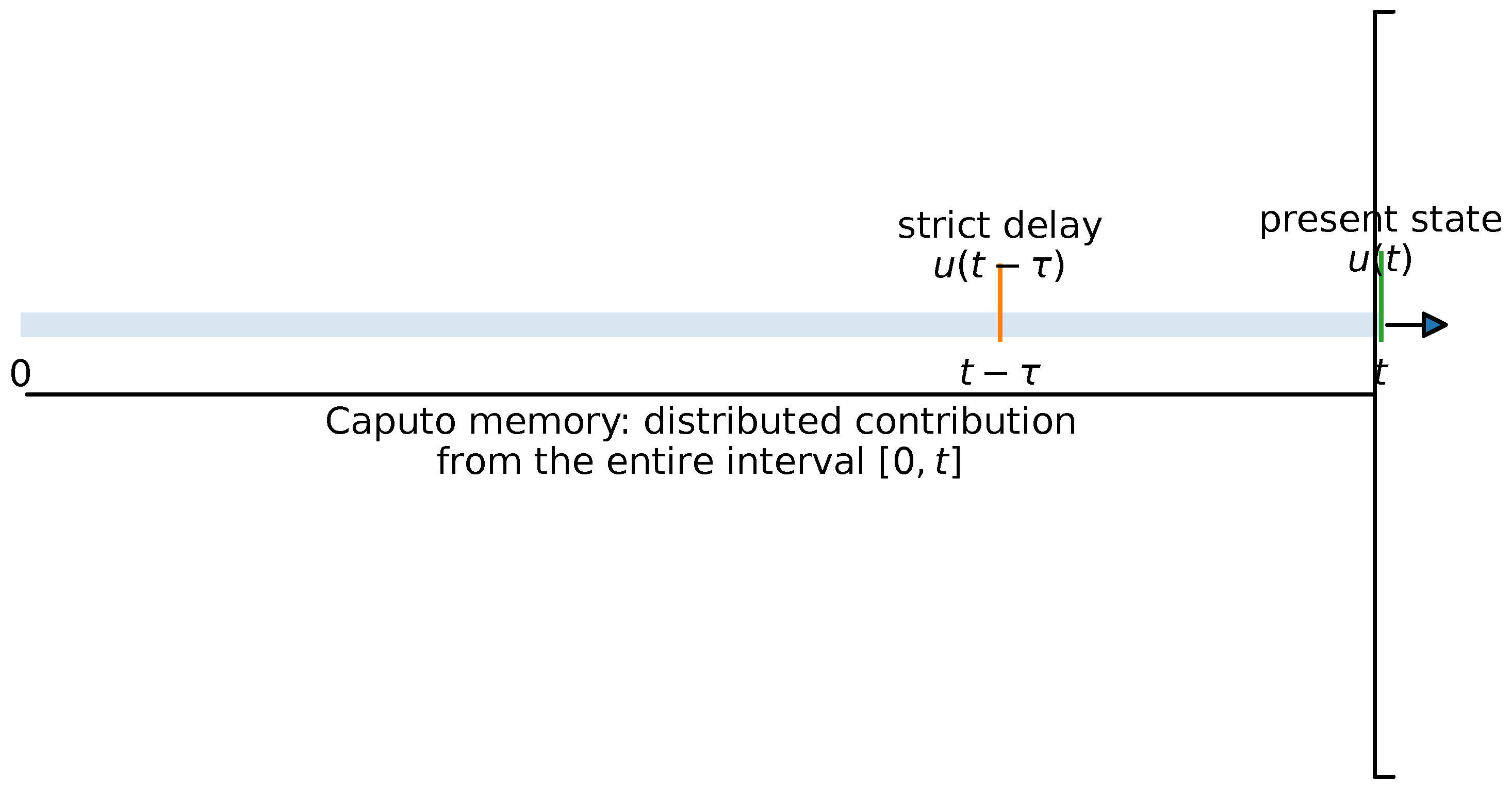
A second memory effect comes from the Caputo derivative. Unlike in the classical parabolic case, the evolution cannot be restarted independently at the endpoints of the delay intervals. The Volterra memory generated by the Caputo operator remains tied to the whole past interval $[0,t]$, while the nonlinear source samples the single delayed time $t-\tau$. The analysis therefore keeps these two forms of memory separate: the continuous memory of the fractional derivative and the discrete memory introduced by the delay. This separation is used because the fractional time derivative determines the Volterra resolvent, the Mittag–Leffler kernels and the energy-decay scale used in the proofs. Figure 1 schematically displays the two time dependencies.

The prototype considered below has the form

$${}^{C}D_t^{\alpha }u+{(-\Delta )}_D^{s}u=\lambda u{(t-\tau )}^p-\mu u{\left(t\right)}^q,$$

with a homogeneous Dirichlet boundary condition and a nonnegative history on $[-\tau ,0]$.

The projection method used here is inspired by the classical first-eigenfunction approach by Kaplan [1] and by Fujita’s work on critical nonlinear parabolic behavior [2]. The methodological connection is that projection onto the positive principal eigenfunction converts a PDE inequality into a scalar inequality, while Fujita’s work provides the classical semilinear diffusion context for nonlinear growth and blow-up behavior. In the present delayed problem, however, the source is evaluated at $t-\tau$ rather than at the current time, so the classical same-time feedback is replaced by an interval-to-interval transfer. Standard background on semilinear parabolic problems is given in [3,4,5]. For fractional equations, we use the frameworks in [6,7,8]; the Mittag–Leffler scale, which replaces exponential decay in many fractional models, is discussed in [9]. We also use comparison and maximum principle ideas from [10,11,12].

The diffusion operator is the spectral fractional power of the Dirichlet Laplacian. Because this operator is defined through the Dirichlet eigenbasis, the first eigenfunction can be used consistently as a positive test mode in the scalar estimates below. This spectral realization should not be confused with the integral fractional Laplacian. In the present work, the exponent s enters explicitly into the spectral gap ${\lambda }_1^s$, the fractional energy form and the small-data decay condition. We refer to [13,14,15] for fractional Sobolev and nonlocal-operator background, and to [16,17] for spectral fractional powers of elliptic operators. Recent works on time-fractional reaction–diffusion equations, including global existence, blow-up and critical behavior, include [18,19,20,21]. For a numerical analysis of Riesz space-fractional reaction–diffusion equations with one or several discrete delays, see [22,23]; these works concern a different spatial realization and an integer-order time derivative, but they provide a directly related numerical comparison for the space-fractional delay component.

Delay and memory have their own analytical tradition. Halanay’s stability estimate [24], the theory of functional differential equations [25], and the Volterra framework in [26] provide background for the present setting. For recent delayed time-fractional reaction–diffusion equations and fractional Halanay estimates, see [27,28].

This combination arises in models in which transport is anomalous while the reaction is activated after a finite response time. Examples include hereditary diffusion with delayed control, maturation or incubation effects in population models, and thermal or viscoelastic media in which the constitutive memory is continuous but the feedback device acts after a prescribed lag. These examples motivate the coexistence of a Caputo memory kernel and a strict delay; the present article develops the analytical consequences of that coexistence rather than a calibrated model for one particular application.

The position of the main results relative to the related strands of the literature is summarized in

Table 1. Theorem-level comparison with explicitly identified nearby works cited in the manuscript.

Related Strand	Typical Result in the Cited Literature	Result Established Here
Delayed Caputo reaction–diffusion [27]	Well-posedness or stability for delayed fractional equations under abstract Lipschitz assumptions	Theorem 1: local well-posedness in the strongly continuous Dirichlet phase space $C_0(\Omega )$, positivity, weak formulation, and a continuation criterion without restarting the Caputo memory
Fractional Halanay asymptotics [28] (Theorem 2.4)	Decay for scalar or abstract delay inequalities	Theorem 3: the weak PDE energy is shown directly, in the distributional Caputo sense, to satisfy a generalized fractional Halanay inequality
Time–space fractional blow-up alternatives [20,21]	Same-time nonlinear production and blow-up/global alternatives	Theorem 2: a strict delay yields an explicit interval-by-interval lower-bound transfer, not a same-time Kaplan blow-up inequality
Space-fractional delay equations [22,23]	Stability and convergence of numerical schemes for Riesz space-fractional reaction–diffusion equations with discrete delays and an integer-order time derivative	The present paper treats a Caputo time derivative, the spectral Dirichlet fractional Laplacian, and a nonlinear strict delay; its main contribution is analytical, while the spectral-Galerkin/L1 experiment is explicitly illustrative rather than a convergence theorem

. The comparison is made at theorem level and is limited to the properties actually proved here.

The works cited above address different subsets of these features rather than their simultaneous occurrence. In this setting, the delay prevents the usual first-eigenfunction projection from producing a same-time nonlinear lower inequality. The resulting estimate is instead a transfer of lower bounds from one delay interval to the next. In the dissipative case, the argument is different and relies on smallness, spectral damping and a fractional Halanay estimate. Thus, this paper belongs to the fractional reaction–diffusion setting both through the time operator and through the spatial diffusion operator.

We study the problem

$$\left\{\begin{array}{cc}{}^{C}D_t^{\alpha }u(x,t)+{(-\Delta )}_D^{s}u(x,t)=\lambda u{(x,t-\tau )}^p-\mu u{(x,t)}^q,\hfill & x\in \Omega ,t>0,\hfill \\ u(x,t)=0,\hfill & x\in \partial \Omega ,t>0,\hfill \\ u(x,t)=\phi (x,t)\ge 0,\hfill & x\in \Omega ,-\tau \le t\le 0,\hfill \end{array}\right.$$

(1)

where $\Omega \subset {\mathbb{R}}^N$ is a bounded, connected domain with $C^{1,1}$ boundary, $0<\alpha <1$, $0<s<1$, $\tau >0$, $\lambda >0$, $\mu \ge 0$ and $p,q>1$. Connectedness ensures the simplicity of the first Dirichlet eigenvalue and allows the corresponding eigenfunction to be chosen strictly positive throughout $\Omega$, as required by the first-mode arguments. The delayed power $u{(t-\tau )}^p$ is the production term. It is fed either by the prescribed history or by values of the solution that have already been constructed. The absorption $u{\left(t\right)}^q$ is not delayed. This is the basic asymmetry in (1).

This asymmetry has a concrete consequence. If the source were $u{\left(t\right)}^p$, the first projection would feed on its own current value and yield a same-time lower scalar inequality. With the strict delay, the source is not allowed to use the current projection. On a given interval of length $\tau$, it uses what was known on the previous interval. For this reason, the delayed-source case with $\mu =0$ leads to a stepwise lower-bound transfer estimate rather than to a same-time scalar blow-up criterion.

This analysis gives three main results. First, nonnegative histories in $C([-\tau ,0];C_0(\Omega ))$ generate nonnegative mild solutions, and boundedness in the $C_0(\Omega )$ norm is the continuation criterion. Second, in the delayed-source case $\mu =0$, the solution exists globally, remains bounded on every finite time interval, and exhibits a stepwise transfer of positive lower bounds for the first Dirichlet mode. Third, when $\mu >0$, $p>q>1$, and the history satisfies the explicit smallness conditions of Theorem 3, the present absorption and the spectral gap dominate the delayed feedback, giving global boundedness and convergence to zero in $L^2(\Omega )$ with a Mittag–Leffler-type decay estimate.

The numerical section has two clearly separated components. The scalar first-mode equation is used only as a heuristic surrogate and is not claimed to be a PDE comparison equation in the dissipative case. Independently, a sine spectral-Galerkin/L1 approximation of the original one-dimensional PDE is reported with temporal and mode refinements; this experiment illustrates the analytical regime but is not promoted to a fully discrete convergence theorem.

To fix the scope of the paper, we emphasize that attractors, $\omega$-limit sets, stationary states and a complete dynamical-system description of (1) are outside the present study. The word “global” is used only in the sense of the global continuation or global boundedness of the solutions considered here. Likewise, “decay” always refers to convergence to zero as $t\to +\infty$, not to finite-time extinction.

This paper is organized as follows. Section 2 fixes the spectral setting, the delayed trajectory and the basic inequalities. Section 3 states the main results. Section 4 proves local existence, positivity and continuation. Section 5 derives the first-mode identities and delayed scalar estimates. Section 6 handles the delayed-source case $\mu =0$. Section 7 proves boundedness and asymptotic decay in the dissipative regime. Section 8 records the Mittag–Leffler and spectral consequences. Section 9 presents the heuristic reduced first-mode illustrations and an independent spatially resolved spectral-Galerkin/L1 PDE computation with refinement studies, and the Section 10 concludes the paper.

2. Functional Setting and Preliminary Estimates

The purpose of this section is not to develop a general theory of spectral fractional operators, but to fix the precise framework needed for the delayed estimates used below. The notation is therefore chosen for the arguments to come. The first eigenfunction will be used to derive scalar lower estimates, while the delayed state specifies whether the source is evaluated on the prescribed history or on a previously constructed portion of the solution. The fractional character of the problem enters here through two independent objects: the Caputo memory kernel in time and the spectral fractional form associated with $A^s$.

Let $\Omega \subset {\mathbb{R}}^N$ be a bounded, connected domain with $C^{1,1}$ boundary. We denote by $C_0(\Omega )$ the Banach space of continuous functions on $\overline{\Omega }$ that vanish on $\partial \Omega$, equipped with the supremum norm. We write $A=-{\Delta }_D$ for the Dirichlet Laplacian in $L^2(\Omega )$, and denote its eigenpairs by ${({\lambda }_k,{\varphi }_k)}_{k\ge 1}$:

$$-\Delta {\varphi }_k={\lambda }_k{\varphi }_k\mathrm{in}\Omega ,{\varphi }_k=0\mathrm{on}\partial \Omega .$$

The eigenvalues are ordered by

$$0<{\lambda }_1<{\lambda }_2\le {\lambda }_3\le \cdots ,{\lambda }_k\to +\infty ,$$

and the eigenfunctions are orthonormal in $L^2(\Omega )$. We choose ${\varphi }_1>0$ in $\Omega$ and normalize it by

$${∥{\varphi }_1∥}_{L^2(\Omega )}=1,M_1={\int }_{\Omega }{\varphi }_1\left(x\right)dx>0.$$

For $0<s<1$, the operator used in the paper is the spectral fractional power of A. Thus, if $u={\sum }_{k\ge 1}{u}_k{\varphi }_k$, then

$$A^{s}u={(-\Delta )}_D^{s}u=\sum _{k\ge 1}{\lambda }_k^s{u}_k{\varphi }_k.$$

The energy space attached to this operator is

$$H_D^s(\Omega )=D\left(A^{s/2}\right)=\left\{u=\sum _{k\ge 1}{u}_k{\varphi }_k\in L^2(\Omega ):\sum _{k\ge 1}{\lambda }_k^s{\left|u_k\right|}^2<+\infty \right\}.$$

Throughout the paper, $H_D^s(\Omega )=D\left(A^{s/2}\right)$ denotes the spectral fractional space associated with the Dirichlet Laplacian. The homogeneous Dirichlet condition is encoded through this spectral construction. This space should not be confused with the integral fractional Sobolev space defined by the Gagliardo seminorm. We use the form

$${\mathcal{E}}_s(u,v)=\sum _{k\ge 1}{\lambda }_k^s{u}_k{v}_k,u,v\in H_D^s(\Omega ),$$

so that

$${\mathcal{E}}_s(u,u)\ge {\lambda }_1^s{∥u∥}_{L^2(\Omega )}^2,u\in H_D^s(\Omega ).$$

The following result collects the truncation and Caputo inequalities used later in the positivity and barrier arguments.

Lemma 1.

Let $H=L^2(\Omega )$, $V=H_D^s(\Omega )$ and $V^{\prime }=H_D^s{(\Omega )}^{\prime }$, with $V\hookrightarrow H\hookrightarrow V^{\prime }$. Assume that

$$v\in C([0,T];H)\cap L^2(0,T;V),v_0=v\left(0\right)\in H,$$

and

$$w:=g_{1-\alpha }\ast (v-v_0)\in H^1(0,T;V^{\prime }),{}^{C}D_t^{\alpha }v=w^{\prime }\in L^2(0,T;V^{\prime }).$$

Then, for every $k\ge 0$, ${(v-k)}^{+}$ and $v^{-}$ belong to $L^2(0,T;V)$. Moreover,

$$g_{1-\alpha }\ast \left({\parallel (v-k)}^{+}{\parallel }_2^2-{\parallel {(v_0-k)}^{+}\parallel }_2^2\right),g_{1-\alpha }\ast \left(\parallel v^{-}{\parallel }_2^2-{\parallel v_0^{-}\parallel }_2^2\right),g_{1-\alpha }\ast \left({\parallel v\parallel }_2^2-{\parallel v_0\parallel }_2^2\right)$$

belong to $W^{1,1}(0,T)$ and, in ${\mathcal{D}}^{\prime }(0,T)$,

$$\begin{array}{cc}\hfill {\langle {}^{C}D_t^{\alpha }v,{(v-k)}^{+}\rangle }_{V^{\prime },V}& \ge {\displaystyle \frac{1}{2}}{\mathfrak{D}}_t^{\alpha }{\parallel {(v-k)}^{+}\parallel }_{L^2(\Omega )}^2,\hfill \end{array}$$

(2)

$$\begin{array}{cc}\hfill {\langle {}^{C}D_t^{\alpha }v,-v^{-}\rangle }_{V^{\prime },V}& \ge {\displaystyle \frac{1}{2}}{\mathfrak{D}}_t^{\alpha }{\parallel v^{-}\parallel }_{L^2(\Omega )}^2,\hfill \end{array}$$

(3)

$$\begin{array}{cc}\hfill {\langle {}^{C}D_t^{\alpha }v,v\rangle }_{V^{\prime },V}& \ge {\displaystyle \frac{1}{2}}{\mathfrak{D}}_t^{\alpha }{\parallel v\parallel }_{L^2(\Omega )}^2.\hfill \end{array}$$

(4)

For a.e. t, the spectral Dirichlet form satisfies

$$\begin{array}{cc}\hfill {\mathcal{E}}_s(v,{(v-k)}^{+})& \ge {\mathcal{E}}_s({(v-k)}^{+},{(v-k)}^{+}),\hfill \end{array}$$

(5)

$$\begin{array}{cc}\hfill {\mathcal{E}}_s(v,-v^{-})& \ge {\mathcal{E}}_s(v^{-},v^{-}).\hfill \end{array}$$

(6)

Consequently, ${(v-k)}^{+}$, $-v^{-}$ and v are admissible tests in the weak inequalities used below.

Proof. 

Let $Bz={\displaystyle \frac{d}{dt}}(g_{1-\alpha }\ast z)$ be the Volterra derivative with zero initial trace, acting in $V^{\prime }$, and let $B_n=nB{(n+B)}^{-1}$ be its Yosida approximation. The standard regularization theory for abstract Volterra equations provides kernels $g_{1-\alpha ,n}\in W^{1,1}(0,T)$ that are nonnegative and nonincreasing, satisfy

$$B_{n}z={\displaystyle \frac{d}{dt}}(g_{1-\alpha ,n}\ast z),g_{1-\alpha ,n}⟶g_{1-\alpha }\mathrm{in}{L}^1(0,T),$$

and give $B_{n}z\to Bz$ strongly for z in the domain of B; see [29,30,31]. Apply this construction to $z=v-v_0$.

For a convex $C^1$ function $\mathsf{\Phi }$ with Lipschitz derivative, the fundamental identity for the regular kernel gives, after integration over $\Omega$,

$${〈B_n(v-v_0),{\mathsf{\Phi }}^{\prime }\left(v\right)〉}_{V^{\prime },V}\ge {\displaystyle \frac{d}{dt}}\left[g_{1-\alpha ,n}\ast {\int }_{\Omega }\left(\mathsf{\Phi }\left(v\right)-\mathsf{\Phi }\left(v_0\right)\right)dx\right]$$

(7)

in the distributional sense. The omitted remainder is nonnegative because $g_{1-\alpha ,n}$ is nonincreasing and $\mathsf{\Phi }$ is convex. Approximate the convex functions

$${\mathsf{\Phi }}_k\left(r\right)=\frac{1}{2}{\left({(r-k)}^{+}\right)}^2,{\mathsf{\Phi }}_{-}\left(r\right)=\frac{1}{2}{\left(r^{-}\right)}^2,{\mathsf{\Phi }}_0\left(r\right)=\frac{1}{2}{r}^2$$

by smooth convex functions with uniformly Lipschitz derivatives. The normal-contraction property of the spectral Dirichlet form implies that the corresponding derivatives belong to V and that the contractions converge strongly in $L^2(0,T;V)$. Since $B_n(v-v_0)\to {}^{C}D_t^{\alpha }v$ in $L^2(0,T;V^{\prime })$, the $L^2\left(V^{\prime }\right)$–$L^2\left(V\right)$ duality permits passage first in the smooth approximation and then as $n\to \infty$. This yields (2)–(4) and the asserted $W^{1,1}$ regularity of the scalar convolutions.

Finally, the form associated with $A^s$ is a symmetric Dirichlet form. Its Markov property gives stability under normal contractions and Inequalities (5)–(6); see [32,33]. □

For a Banach-space-valued function y, the vector-valued Caputo derivative used in the weak formulation is defined by Bochner convolution:

$${}^{C}D_t^{\alpha }y={\displaystyle \frac{d}{dt}}\left[g_{1-\alpha }\ast (y-y\left(0\right))\right],g_{1-\alpha }\left(t\right)={\displaystyle \frac{t^{-\alpha }}{\mathsf{\Gamma }(1-\alpha )}},$$

whenever the convolution belongs to the relevant Bochner–Sobolev space. For a continuous scalar function z whose convolution belongs to $W_{\mathrm{loc}}^{1,1}(0,T)$, we write separately

$${\mathfrak{D}}_t^{\alpha }z:={\displaystyle \frac{d}{dt}}\left[g_{1-\alpha }\ast (z-z\left(0\right))\right]\mathrm{in}{\mathcal{D}}^{\prime }(0,T).$$

When y is absolutely continuous, the vector-valued definition agrees with the classical formula

$${}^{C}D_t^{\alpha }y\left(t\right)={\displaystyle \frac{1}{\mathsf{\Gamma }(1-\alpha )}}{\int }_0^t{(t-\xi )}^{-\alpha }{y}^{\prime }\left(\xi \right)d\xi .$$

The lower limit is fixed at 0 in both notations; hence, the Volterra memory is never restarted at the endpoints of the delay intervals.

We also use the Mittag–Leffler functions

$$E_{\alpha ,\beta }\left(z\right)={\displaystyle \sum _{n=0}^{\infty }}{\displaystyle \frac{z^n}{\mathsf{\Gamma }(\alpha n+\beta )}},E_{\alpha }\left(z\right)=E_{\alpha ,1}\left(z\right).$$

They are the kernels naturally associated with the linear Caputo equation and are used both in the lower first-mode estimates and in the decay bounds.

The past is prescribed on an interval, not only at one initial time:

$$\phi \in C([-\tau ,0];C_0(\Omega )),\phi \ge 0.$$

We keep the compatibility condition

$$u(x,0)=\phi (x,0)\mathrm{for}\mathrm{a}.\mathrm{e}.x\in \Omega .$$

For positive times, the history is attached to the trajectory by

$$\tilde{u}(x,t)=\left\{\begin{array}{cc}\phi (x,t),\hfill & -\tau \le t\le 0,\hfill \\ u(x,t),\hfill & t>0,\hfill \end{array}\right.$$

and the delayed state is

$$u_{\tau }(x,t)=\tilde{u}(x,t-\tau ).$$

Thus,

$$u_{\tau }(x,t)=\left\{\begin{array}{cc}\phi (x,t-\tau ),\hfill & 0<t<\tau ,\hfill \\ u(x,t-\tau ),\hfill & t\ge \tau .\hfill \end{array}\right.$$

At a time t, the source therefore reads either the prescribed history or a value which has already been produced by the evolution.

For later use and to fix the notation for weak solutions, we rewrite (1) as

$$\left\{\begin{array}{cc}{}^{C}D_t^{\alpha }u(x,t)+A^{s}u(x,t)=\lambda u_{\tau }{(x,t)}^p-\mu u{(x,t)}^q,\hfill & x\in \Omega ,t>0,\hfill \\ u(x,t)=0,\hfill & x\in \partial \Omega ,t>0,\hfill \\ u(x,t)=\phi (x,t),\hfill & x\in \Omega ,-\tau \le t\le 0.\hfill \end{array}\right.$$

(8)

Definition 1.

Let $T>0$, $V=H_D^s(\Omega )$, and $V^{\prime }=H_D^s{(\Omega )}^{\prime }$. A nonnegative function u is a weak solution of (8) on $(0,T)$ if

$$u\in C([0,T];L^2(\Omega ))\cap L^2(0,T;V),g_{1-\alpha }\ast (u-u\left(0\right))\in H^1(0,T;V^{\prime }),$$

so that

$${}^{C}D_t^{\alpha }u={\displaystyle \frac{d}{dt}}\left[g_{1-\alpha }\ast (u-u\left(0\right))\right]\in L^2(0,T;V^{\prime }),$$

and if $u_{\tau }^p,u^q\in L^2(0,T;L^2(\Omega ))$. For every $\psi \in V$ and a.e. $t\in (0,T)$,

$${\langle {}^{C}D_t^{\alpha }u\left(t\right),\psi \rangle }_{V^{\prime },V}+{\mathcal{E}}_s(u\left(t\right),\psi )=\lambda {\int }_{\Omega }{u}_{\tau }{(x,t)}^p\psi \left(x\right)dx-\mu {\int }_{\Omega }u{(x,t)}^q\psi \left(x\right)dx.$$

(9)

Moreover, $u=\phi$ on $\Omega \times [-\tau ,0]$ and $u\left(0\right)=\phi \left(0\right)$ in $L^2(\Omega )$.

For later use, we also recall the mild representation associated with the linear Caputo equation. Define the operators

$$S_{\alpha }\left(t\right)v={\displaystyle \sum _{k=1}^{\infty }}{E}_{\alpha }(-{\lambda }_k^s{t}^{\alpha })v_k{\varphi }_k,v={\displaystyle \sum _{k=1}^{\infty }}{v}_k{\varphi }_k,$$

and

$$P_{\alpha }\left(t\right)v={\displaystyle \sum _{k=1}^{\infty }}{t}^{\alpha -1}{E}_{\alpha ,\alpha }(-{\lambda }_k^s{t}^{\alpha })v_k{\varphi }_k.$$

For bounded source terms, the associated mild formulation is

$$u\left(t\right)=S_{\alpha }\left(t\right)\phi \left(0\right)+{\int }_0^t{P}_{\alpha }(t-\xi )\left[\lambda u_{\tau }{\left(\xi \right)}^p-\mu u{\left(\xi \right)}^q\right]d\xi .$$

We shall also use Jensen’s inequality with the first eigenfunction as a positive weight.

Lemma 2.

Let $r>1$ and let $v\ge 0$ a.e. in Ω. Then,

$${\int }_{\Omega }v{\left(x\right)}^r{\varphi }_1\left(x\right)dx\ge M_1^{1-r}{\left({\int }_{\Omega }v\left(x\right){\varphi }_1\left(x\right)dx\right)}^r.$$

(10)

Proof. 

Set

$$d\nu \left(x\right)={\displaystyle \frac{{\varphi }_1\left(x\right)}{M_1}}dx.$$

Then, $\nu$ is a probability measure on $\Omega$. Since $z\mapsto z^r$ is convex on $[0,+\infty )$, Jensen’s inequality gives

$${\int }_{\Omega }v{\left(x\right)}^{r}d\nu \left(x\right)\ge {\left({\int }_{\Omega }v\left(x\right)d\nu \left(x\right)\right)}^r.$$

Multiplying by $M_1$ yields (10). □

3. Statement of the Main Results

We now state the main results. All notation is that of Section 2. In particular, $A^s={(-\Delta )}_D^s$ denotes the spectral fractional Dirichlet Laplacian, ${\varphi }_1$ is the positive first Dirichlet eigenfunction normalized in $L^2(\Omega )$, and

$$M_1={\int }_{\Omega }{\varphi }_1\left(x\right)dx.$$

The delayed state is $u_{\tau }(x,t)=\tilde{u}(x,t-\tau )$, where $\tilde{u}$ is the historical extension associated with $\phi$.

The results below have complementary roles. The first one gives the local well-posedness and continuation framework for the Caputo–spectral fractional Volterra formulation. The second one describes the stepwise lower-bound transfer produced by the strict delay in the case $\mu =0$. The third one gives global boundedness and fractional Mittag–Leffler decay when the delayed feedback is dominated by present absorption and spectral damping.

The term “delayed transfer” refers only to the propagation of positive lower bounds from the history window to the first spectral mode, and then from one delay interval to the next. It is not a finite-time blow-up statement.

We first record the local well-posedness and continuation framework.

Theorem 1.

Assume that

$$\phi \in C([-\tau ,0];C_0(\Omega )),\phi \ge 0.$$

Then, Problem (8) admits a unique maximal nonnegative mild solution

$$u\in C([-\tau ,T_{\max });C_0(\Omega )),$$

where $T_{\max }\in (0,+\infty ]$. Moreover, for every $T<T_{\max }$, the restriction of u to $(0,T)$ satisfies the weak formulation of Definition 1. If $T_{\max }<+\infty$, then

$$\underset{t\uparrow T_{\max }}{lim\; sup}{∥u\left(t\right)∥}_{C_0(\Omega )}=+\infty .$$

This result provides the local well-posedness framework for the delayed Volterra formulation. The continuation criterion is used below to convert finite-interval bounds into global-in-time continuation.

The next result treats the case $\mu =0$ and gives the stepwise transfer of first-mode lower bounds.

Theorem 2.

Assume that $\mu =0$. Let u be the maximal nonnegative solution of (8). Then,

$$T_{\max }=+\infty .$$

Moreover, for every $T>0$,

$$\underset{0\le t\le T}{sup}{∥u\left(t\right)∥}_{C_0(\Omega )}<+\infty .$$

Furthermore, assume

$${\eta }_0:=\underset{-\tau \le \theta \le 0}{\min }{m}_{\phi }\left(\theta \right)>0,m_{\phi }\left(\theta \right)={\int }_{\Omega }\phi (x,\theta ){\varphi }_1\left(x\right)dx.$$

Let $a={\lambda }_1^s$ and $b=\lambda M_1^{1-p}$. Define recursively

$$L_{n+1}\left(t\right)=m\left(0\right)E_{\alpha }(-a{t}^{\alpha })+b{\eta }_n^p{\int }_{n\tau }^t{(t-\xi )}^{\alpha -1}{E}_{\alpha ,\alpha }(-a{(t-\xi )}^{\alpha })d\xi ,$$

for $n\tau \le t\le (n+1)\tau$, and

$${\eta }_{n+1}=\underset{n\tau \le t\le (n+1)\tau }{\min }{L}_{n+1}\left(t\right)>0.$$

Then, the history satisfies $m_{\phi }\left(\theta \right)\ge {\eta }_0$ on $[-\tau ,0]$, and, for every $n\ge 1$,

$$m\left(t\right)\ge {\eta }_n,(n-1)\tau \le t\le n\tau .$$

In particular, the positive first-mode lower bound propagates recursively through every delay interval.

The estimate on the first interval records the first transfer of historical mass into the solution. The second estimate shows how the same transfer repeats from one delay interval to the next. This is the precise sense in which the first-mode lower-bound transfer is delayed and stepwise.

The final main result gives global boundedness and decay under a dissipative smallness condition.

Theorem 3.

Assume that

$$\mu >0,p>q>1.$$

Let $\epsilon >0$ exist such that

$$\lambda {\epsilon }^{p-q}\le \mu \mathrm{and}\lambda {\epsilon }^{p-1}<{\lambda }_1^s.$$

Such a choice of ε is possible by taking $\epsilon >0$ sufficiently small, since $p>q>1$; histories satisfying the barrier below are then admissible. If the history satisfies

$$0\le \phi (x,t)\le \epsilon ,\mathit{for}a.e.x\in \Omega ,-\tau \le t\le 0,$$

then the corresponding solution is global and satisfies

$$0\le u(x,t)\le \epsilon ,\mathit{for}a.e.x\in \Omega ,t\ge -\tau .$$

Furthermore,

$${∥u\left(t\right)∥}_{L^2(\Omega )}\to 0\mathit{as}t\to +\infty .$$

More precisely, let

$$\gamma =2{\lambda }_1^s-\lambda {\epsilon }^{p-1},\delta =\lambda {\epsilon }^{p-1},$$

and let ${\omega }_{*}>0$ be the unique root of

$${\omega }_{*}-\gamma +{\displaystyle \frac{\delta }{E_{\alpha }(-{\omega }_{*}{\tau }^{\alpha })}}=0.$$

Then, every $0<\omega <{\omega }_{*}$ is admissible and

$${∥u\left(t\right)∥}_{L^2(\Omega )}^2\le C{E}_{\alpha }(-\omega t^{\alpha }),t\ge 0,C=\underset{-\tau \le \theta \le 0}{sup}{∥\phi \left(\theta \right)∥}_{L^2(\Omega )}^2.$$

The two smallness conditions have distinct roles. The condition $\lambda {\epsilon }^{p-q}\le \mu$ ensures the invariance of the barrier $0\le u\le \epsilon$, since under this barrier the present absorption dominates the delayed source. The condition $\lambda {\epsilon }^{p-1}<{\lambda }_1^s$ provides a dominant dissipative contribution in the energy inequality and allows the application of a fractional Halanay-type argument. The condition $p>q>1$ ensures that, near the origin, the delayed source $u_{\tau }^p$ is of higher order than the present absorption $u^q$; hence, it can be dominated under a sufficiently small invariant barrier. These conditions are sufficient and are not asserted to be sharp. Retaining the absorption term in the energy estimate may enlarge the stability region, but no closed estimate depending only on $Y\left(t\right)$ and its delayed supremum follows in general from the projection inequalities available here; optimization of the stability region is left open.

The two regimes described above are complementary. Without instantaneous absorption, the delayed source yields a stepwise transfer of lower bounds through the first Dirichlet mode. When the two smallness conditions of Theorem 3 hold, the delayed feedback is dominated by the spectral gap and the solution decays to zero.

4. Proof of Local Existence, Positivity and Continuation

This section proves Theorem 1. We first construct a local mild solution by a fixed-point argument for a truncated equation. We then justify the weak formulation of the truncated solution. The positivity test is performed at this level, which avoids a circular use of the weak formulation. Finally, we establish the continuation criterion in the supremum norm of $C_0(\Omega )$.

The mild form of (8) is

$$u\left(t\right)=S_{\alpha }\left(t\right)\phi \left(0\right)+{\int }_0^t{P}_{\alpha }(t-\xi )\left[\lambda u_{\tau }{\left(\xi \right)}^p-\mu u{\left(\xi \right)}^q\right]d\xi .$$

4.1. Local Construction

The proof of local existence is performed with a truncated nonlinearity. Define

$$F(v,w)=\lambda {\left(w^{+}\right)}^p-\mu {\left(v^{+}\right)}^q,v,w\in \mathbb{R},$$

where $z^{+}=\max \{z,0\}$. On every bounded subset of ${\mathbb{R}}^2$, the function F is locally Lipschitz. Once positivity is established, the truncated equation coincides with the original problem.

Let

$$R_0={∥\phi ∥}_{C([-\tau ,0];C_0(\Omega ))}.$$

Choose $R>2R_0$. For $T>0$, set

$$X_T=\left\{v\in C([-\tau ,T];C_0(\Omega )):v\left(t\right)=\phi \left(t\right)\mathrm{for}-\tau \le t\le 0,{∥v∥}_{C([-\tau ,T];C_0)}\le R\right\}.$$

For $v\in X_T$, let $v_{\tau }\left(t\right)=\tilde{v}(t-\tau )$ be the delayed state associated with the historical extension of v. Define the operator $\mathcal{T}$ by

$$\left(\mathcal{T}v\right)\left(t\right)=\phi \left(t\right),-\tau \le t\le 0,$$

and, for $0<t\le T$,

$$\left(\mathcal{T}v\right)\left(t\right)=S_{\alpha }\left(t\right)\phi \left(0\right)+{\int }_0^t{P}_{\alpha }(t-\xi )F(v\left(\xi \right),v_{\tau }\left(\xi \right))d\xi .$$

(11)

The linear operators used in (11) satisfy the properties needed for the fixed-point argument. Let $T_s\left(r\right)=e^{-r{A}^s}$ be the positive contraction semigroup generated by $-A^s$ on $C_0(\Omega )$. With the standard Wright density ${\mathsf{\Phi }}_{\alpha }\ge 0$, the subordinated families are

$$S_{\alpha }\left(t\right)z={\int }_0^{\infty }{\mathsf{\Phi }}_{\alpha }\left(\theta \right)T_s\left(t^{\alpha }\theta \right)zd\theta ,$$

$$P_{\alpha }\left(t\right)z=\alpha t^{\alpha -1}{\int }_0^{\infty }\theta {\mathsf{\Phi }}_{\alpha }\left(\theta \right)T_s\left(t^{\alpha }\theta \right)zd\theta .$$

Since ${\int }_0^{\infty }{\mathsf{\Phi }}_{\alpha }\left(\theta \right)d\theta =1$ and $\alpha {\int }_0^{\infty }\theta {\mathsf{\Phi }}_{\alpha }\left(\theta \right)d\theta =1/\mathsf{\Gamma }\left(\alpha \right)$,

$$\parallel S_{\alpha }{\left(t\right)\parallel }_{\mathcal{L}\left(C_0\right)}\le 1,{\parallel P_{\alpha }\left(t\right)\parallel }_{\mathcal{L}\left(C_0\right)}\le {\displaystyle \frac{t^{\alpha -1}}{\mathsf{\Gamma }\left(\alpha \right)}},t>0.$$

(12)

Consequently, for every $g\in L^{\infty }(0,T_0;C_0(\Omega ))$,

$${∥{\int }_0^t{P}_{\alpha }(t-\xi )g\left(\xi \right)d\xi ∥}_{C_0(\Omega )}\le {\displaystyle \frac{t^{\alpha }}{\mathsf{\Gamma }(1+\alpha )}}{\parallel g\parallel }_{L^{\infty }(0,t;C_0(\Omega ))}.$$

(13)

These formulas also give positivity and strong continuity of $S_{\alpha }$ on $C_0(\Omega )$. Since $-A^s$ generates an analytic Dirichlet semigroup, $S_{\alpha }$ and $P_{\alpha }$ are operator-norm continuous on every compact subinterval of $(0,+\infty )$. Finally, the truncated nonlinearity is locally Lipschitz on every bounded subset of $C_0(\Omega )\times C_0(\Omega )$, since the scalar maps $z\mapsto {\left(z^{+}\right)}^p$ and $z\mapsto {\left(z^{+}\right)}^q$ are locally Lipschitz on bounded intervals.

Since F is bounded on ${[-R,R]}^2$, there exists $C_R>0$ such that

$$\left|F(v,w)\right|\le C_R,\left|v\right|\le R,\left|w\right|\le R.$$

Hence,

$${∥\mathcal{T}v∥}_{C([0,T];C_0)}\le R_0+T^{\alpha }{C}_R/\mathsf{\Gamma }(1+\alpha ).$$

Taking $T>0$ sufficiently small, $\mathcal{T}$ maps $X_T$ into itself.

Since F is Lipschitz on ${[-R,R]}^2$, there exists $L_R>0$ such that

$$|F(v_1,w_1)-F(v_2,w_2)|\le L_R\left(\right|v_1-v_2|+|w_1-w_2\left|\right).$$

Moreover,

$$\parallel {\left(v_1\right)}_{\tau }-{\left(v_2\right)}_{\tau }{\parallel }_{C([0,T];C_0)}\le {\parallel v_1-v_2\parallel }_{C([-\tau ,T];C_0)}.$$

Therefore, for $v_1,v_2\in X_T$,

$${∥\mathcal{T}{v}_1-\mathcal{T}{v}_2∥}_{C([0,T];C_0)}\le 2L_R{T}^{\alpha }/\mathsf{\Gamma }(1+\alpha ){∥v_1-v_2∥}_{C([-\tau ,T];C_0)}.$$

Choosing $T>0$ smaller if necessary, we obtain $2L_R{T}^{\alpha }/\mathsf{\Gamma }(1+\alpha )<1$. The time T is chosen in terms of $R,\lambda ,\mu ,p,q,\alpha ,s$ and $\Omega$ through $L_R$ and the explicit resolvent bound in (12); it is not chosen in terms of the particular function v in the ball $X_T$. Thus, $\mathcal{T}$ is a contraction on $X_T$. Banach’s fixed-point theorem gives a unique mild solution of the truncated delayed problem on $[-\tau ,T]$.

The continuation step is performed without resetting the Caputo memory. One keeps the already constructed trajectory on $[0,T_0]$ in the Volterra integral and applies the same fixed-point estimate to the unknown part on $[T_0,T_0+\theta ]$, with the previous contribution treated as known data. Thus, one obtains a unique maximal mild solution

$$u\in C([-\tau ,T_{\max });C_0(\Omega ))$$

for the truncated equation.

4.2. Weak Formulation for the Truncated Equation

We record the mild-to-weak passage before the use of truncation tests. This avoids using the weak formulation before it has been justified.

Lemma 3.

Let $T<T_{\max }$. The fixed point of (11) belongs to

$$C([0,T];L^2(\Omega ))\cap L^2(0,T;V),g_{1-\alpha }\ast (u-\phi \left(0\right))\in H^1(0,T;V^{\prime }),$$

and satisfies

$$\langle {}^{C}D_t^{\alpha }u\left(t\right),\psi \rangle +{\mathcal{E}}_s(u\left(t\right),\psi )={\int }_{\Omega }F(u\left(t\right),u_{\tau }\left(t\right))\psi \left(x\right)dx$$

(14)

for every $\psi \in V$ and for a.e. $t\in (0,T)$.

Proof. 

Put $f=F(u,u_{\tau })$. Since $u\in C([-\tau ,T];C_0(\Omega ))$, $f\in C([0,T];C_0(\Omega ))\subset L^2(0,T;L^2(\Omega ))$. This passage does not construct a new nonlinear Galerkin scheme: after the mild fixed point has been obtained, f is treated as the prescribed forcing in the linear fractional equation satisfied by u.

Write $f_k\left(t\right)={(f\left(t\right),{\varphi }_k)}_{L^2}$ and $u_{0k}={(\phi \left(0\right),{\varphi }_k)}_{L^2}$. The spectral representation of the mild solution is

$$u\left(t\right)={\displaystyle \sum _{k=1}^{\infty }}{u}_k\left(t\right){\varphi }_k,u_k\left(t\right)=E_{\alpha }(-{\lambda }_k^s{t}^{\alpha })u_{0k}+{\int }_0^t{(t-\xi )}^{\alpha -1}{E}_{\alpha ,\alpha }(-{\lambda }_k^s{(t-\xi )}^{\alpha })f_k\left(\xi \right)d\xi .$$

For $u_m={\sum }_{k=1}^m{u}_k{\varphi }_k$, each coefficient satisfies

$${\mathfrak{D}}_t^{\alpha }{u}_k+{\lambda }_k^s{u}_k=f_k,u_k\left(0\right)=u_{0k}.$$

Testing the first m equations by $u_k$ and summing gives, in the scalar distributional sense,

$${\displaystyle \frac{1}{2}}{\mathfrak{D}}_t^{\alpha }\parallel u_m{\left(t\right)\parallel }_2^2+{\parallel u_m\left(t\right)\parallel }_V^2\le {(P_{m}f\left(t\right),u_m\left(t\right))}_{L^2}.$$

The spectral Poincaré inequality and Young’s inequality imply

$${(P_{m}f,u_m)}_{L^2}\le {\parallel f\parallel }_2{\parallel u_m\parallel }_2\le {\lambda }_1^{-s/2}{\parallel f\parallel }_2{\parallel u_m\parallel }_V\le {\displaystyle \frac{1}{2}}{\parallel u_m\parallel }_V^2+{\displaystyle \frac{1}{2{\lambda }_1^s}}{\parallel f\parallel }_2^2.$$

Consequently,

$${\mathfrak{D}}_t^{\alpha }\parallel u_m{\left(t\right)\parallel }_2^2+\parallel u_m{\left(t\right)\parallel }_V^2\le {\lambda }_1^{-s}{\parallel f\left(t\right)\parallel }_2^2.$$

(15)

Let $I^{\alpha }$ denote the Riemann–Liouville fractional integral. Applying $I^{\alpha }$ to (15) and using $I^{\alpha }{\mathfrak{D}}_t^{\alpha }z\left(t\right)=z\left(t\right)-z\left(0\right)$ gives

$$\parallel u_m{\left(t\right)\parallel }_2^2+I^{\alpha }({\parallel u_m\parallel }_V^2)\left(t\right)\le \parallel P_m{\phi \left(0\right)\parallel }_2^2+{\lambda }_1^{-s}{I}^{\alpha }{(\parallel f\parallel }_2^2)\left(t\right).$$

Since $f\in L^{\infty }(0,T;L^2(\Omega ))$,

$$I^{\alpha }{(\parallel f\parallel }_2^2)\left(t\right)\le {\displaystyle \frac{T^{\alpha }}{\mathsf{\Gamma }(1+\alpha )}}{\parallel f\parallel }_{L^{\infty }(0,T;L^2)}^2.$$

Moreover, for every nonnegative g,

$${\int }_0^{T}g\left(t\right)dt\le \mathsf{\Gamma }\left(\alpha \right)T^{1-\alpha }{I}^{\alpha }g\left(T\right).$$

We therefore obtain

$$\underset{0\le t\le T}{sup}{\parallel u_m\left(t\right)\parallel }_2^2+{\int }_0^T{\parallel u_m\left(t\right)\parallel }_V^{2}dt\le C_T\left({\parallel \phi \left(0\right)\parallel }_2^2+{\parallel f\parallel }_{L^{\infty }(0,T;L^2)}^2\right),$$

(16)

where $C_T$ depends only on $T,\alpha ,s$ and ${\lambda }_1$, and is independent of m. Moreover,

$${\parallel {}^{C}D_t^{\alpha }{u}_m\parallel }_{L^2(0,T;V^{\prime })}\le {\parallel u_m\parallel }_{L^2(0,T;V)}+{\parallel f\parallel }_{L^2(0,T;L^2)}.$$

Because $u\left(\right[0,T\left]\right)$ is compact in $L^2(\Omega )$ and the orthogonal projections $P_m$ converge strongly to the identity, $u_m=P_{m}u\to u$ uniformly in $C([0,T];L^2(\Omega ))$. Bound (16) and the monotone convergence of the spectral energy show that $u\in L^2(0,T;V)$; the spectral tails then give $u_m\to u$ strongly in $L^2(0,T;V)$. Consequently,

$$A^s{u}_m\to A^{s}u\mathrm{in}{L}^2(0,T;V^{\prime }),P_{m}f\to f\mathrm{in}{L}^2(0,T;L^2),$$

and therefore

$${}^{C}D_t^{\alpha }{u}_m=P_{m}f-A^s{u}_m⟶f-A^{s}u\mathrm{in}{L}^2(0,T;V^{\prime }).$$

Passing to the limit in

$${\displaystyle \frac{d}{dt}}\left[g_{1-\alpha }\ast (u_m-P_m\phi \left(0\right))\right]={}^{C}D_t^{\alpha }{u}_m$$

shows that $g_{1-\alpha }\ast (u-\phi \left(0\right))\in H^1(0,T;V^{\prime })$ with derivative $f-A^{s}u$. The finite-dimensional variational identities then yield (14). Finally, convergence in $C([0,T];L^2)$ gives $u\left(0\right)=\phi \left(0\right)$ and identifies the initial trace. Thus, every item in Definition 1 is verified. □

The following positivity argument is therefore justified at the weak level.

4.3. Positivity

We now prove that the solution is nonnegative. Since the history satisfies

$$\phi \ge 0\mathrm{on}\Omega \times [-\tau ,0],$$

it remains to prove nonnegativity for positive times. Let

$$u^{-}(x,t)=\max \{-u(x,t),0\}.$$

The test function $-u^{-}\left(t\right)$ is admissible by Lemma 1. Using it in (14), we obtain

$$\langle {}^{C}D_t^{\alpha }u\left(t\right),-u^{-}\left(t\right)\rangle +{\mathcal{E}}_s(u\left(t\right),-u^{-}\left(t\right))={\int }_{\Omega }F(u\left(t\right),u_{\tau }\left(t\right))(-u^{-}\left(t\right))dx.$$

On the set where $u<0$, one has $u^{+}=0$. Moreover, since the truncated source contains only ${\left(u_{\tau }^{+}\right)}^p$ and ${\left(u^{+}\right)}^q$, we have

$$F(u\left(t\right),u_{\tau }\left(t\right))=\lambda {\left(u_{\tau }^{+}\left(t\right)\right)}^p\ge 0$$

there. Therefore,

$${\int }_{\Omega }F(u\left(t\right),u_{\tau }\left(t\right))(-u^{-}\left(t\right))dx\le 0.$$

By Lemma 1,

$${\mathcal{E}}_s(u\left(t\right),-u^{-}\left(t\right))\ge {\mathcal{E}}_s(u^{-}\left(t\right),u^{-}\left(t\right)),$$

and

$$\langle {}^{C}D_t^{\alpha }u\left(t\right),-u^{-}\left(t\right)\rangle \ge {\displaystyle \frac{1}{2}}{\mathfrak{D}}_t^{\alpha }{∥u^{-}\left(t\right)∥}_{L^2(\Omega )}^2.$$

Consequently,

$${\displaystyle \frac{1}{2}}{\mathfrak{D}}_t^{\alpha }{∥u^{-}\left(t\right)∥}_{L^2(\Omega )}^2+{\mathcal{E}}_s(u^{-}\left(t\right),u^{-}\left(t\right))\le 0.$$

Using the spectral Poincare inequality gives

$${\mathfrak{D}}_t^{\alpha }{∥u^{-}\left(t\right)∥}_{L^2(\Omega )}^2+2{\lambda }_1^s{∥u^{-}\left(t\right)∥}_{L^2(\Omega )}^2\le 0.$$

Since $u^{-}\left(0\right)=0$, convolution with the positive resolvent kernel of ${\mathfrak{D}}_t^{\alpha }+2{\lambda }_1^s$ gives $\parallel u^{-}{\left(t\right)\parallel }_2^2\le 0$. As this quantity is nonnegative,

$${∥u^{-}\left(t\right)∥}_{L^2(\Omega )}^2=0,0\le t<T_{\max }.$$

Thus, $u\ge 0$. Hence, the truncated nonlinearity coincides with the original nonlinearity.

4.4. Weak Formulation for the Original Equation

Let $T<T_{\max }$. Since

$$u\in C([-\tau ,T];C_0(\Omega )),$$

the nonlinear terms $u_{\tau }^p$ and $u^q$ belong to $C([0,T];C_0(\Omega ))$. Since positivity has been proven, Identity (14) becomes exactly

$$\langle {}^{C}D_t^{\alpha }u\left(t\right),\psi \rangle +{\mathcal{E}}_s(u\left(t\right),\psi )=\lambda {\int }_{\Omega }{u}_{\tau }{(x,t)}^p\psi \left(x\right)dx-\mu {\int }_{\Omega }u{(x,t)}^q\psi \left(x\right)dx.$$

Thus, the restriction of u to $(0,T)$ satisfies the weak formulation of Definition 1.

4.5. Continuation Criterion

Assume that $T_{\max }<+\infty$ and

$$M:=\underset{0\le t<T_{\max }}{sup}{\parallel u\left(t\right)\parallel }_{C_0(\Omega )}<+\infty .$$

Set $R=2M+1$. On the ball of radius R, the nonlinearity has a bound $B_R$ and a Lipschitz constant $L_R$ depending only on R and the structural parameters. Put

$$f\left(t\right)=\lambda u_{\tau }{\left(t\right)}^p-\mu u{\left(t\right)}^q,{\parallel f\left(t\right)\parallel }_{C_0}\le B_R,$$

and, for $T_0<T_{\max }$, define

$$G_{T_0}\left(t\right)=S_{\alpha }\left(t\right)\phi \left(0\right)+{\int }_0^{T_0}{P}_{\alpha }(t-\xi )f\left(\xi \right)d\xi ,t\ge T_0.$$

The mild equation gives $G_{T_0}\left(T_0\right)=u\left(T_0\right)$.

We now prove the uniform left-endpoint modulus that is needed for continuation. It is enough to take $T_0\in [T_{\max }/2,T_{\max })$. With $r=T_0-\xi$ and $0\le h\le 1$,

$$\begin{array}{cc}\hfill \parallel G_{T_0}(T_0+h)-G_{T_0}\left(T_0\right){\parallel }_{C_0}& \le {\parallel [S_{\alpha }(T_0+h)-S_{\alpha }\left(T_0\right)]\phi \left(0\right)\parallel }_{C_0}\hfill \\ \hfill & +B_R{\int }_0^{T_0}{\parallel P_{\alpha }(r+h)-P_{\alpha }\left(r\right)\parallel }_{\mathcal{L}\left(C_0\right)}dr.\hfill \end{array}$$

Fix $0<\eta <T_{\max }/2$. On $0<r<\eta$, Bound (12) gives

$${\int }_0^{\eta }\left(\parallel P_{\alpha }(r+h)\parallel +\parallel P_{\alpha }\left(r\right)\parallel \right)dr\le {\displaystyle \frac{2{\eta }^{\alpha }}{\mathsf{\Gamma }(1+\alpha )}}.$$

On $[\eta ,T_{\max }+1]$, the operator-norm continuity of $P_{\alpha }$ is uniform, while the corresponding $S_{\alpha }$ term is uniform for $T_0\in [T_{\max }/2,T_{\max }]$. First, choose $\eta$ small and then h small. We obtain a function $\rho :[0,1]\to [0,+\infty )$, independent of $T_0$, such that

$$\underset{0\le h\le \delta }{sup}\parallel G_{T_0}(T_0+h)-u\left(T_0\right){\parallel }_{C_0(\Omega )}\le \rho \left(\delta \right),\rho \left(\delta \right)\downarrow 0(\delta \downarrow 0).$$

(17)

Choose ${\delta }_{*}>0$, independently of $T_0$, so that

$$\rho \left({\delta }_{*}\right)+{\displaystyle \frac{B_R{\delta }_{*}^{\alpha }}{\mathsf{\Gamma }(1+\alpha )}}\le 1,{\displaystyle \frac{2L_R{\delta }_{*}^{\alpha }}{\mathsf{\Gamma }(1+\alpha )}}<1,{\delta }_{*}\le \tau .$$

Let

$${\mathcal{B}}_{T_0}=\left\{v\in C([T_0,T_0+{\delta }_{*}];C_0(\Omega )):\underset{T_0\le t\le T_0+{\delta }_{*}}{sup}{\parallel v\left(t\right)-u\left(T_0\right)\parallel }_{C_0}\le 1\right\},$$

and attach to v the known trajectory on $[-\tau ,T_0]$. For $t\in [T_0,T_0+{\delta }_{*}]$, define

$$\left(\mathcal{K}v\right)\left(t\right)=G_{T_0}\left(t\right)+{\int }_{T_0}^t{P}_{\alpha }(t-\xi )[\lambda v_{\tau }{\left(\xi \right)}^p-\mu v{\left(\xi \right)}^q]d\xi .$$

Estimates (13) and (17) show that $\mathcal{K}$ maps ${\mathcal{B}}_{T_0}$ into itself, while the second displayed inequality makes it a contraction. All constants and ${\delta }_{*}$ are independent of $T_0$. Taking $T_0>T_{\max }-{\delta }_{*}/2$ extends the solution beyond $T_{\max }$, which is a contradiction. Hence,

$$\underset{t\uparrow T_{\max }}{lim\; sup}{\parallel u\left(t\right)\parallel }_{C_0(\Omega )}=+\infty .$$

The proof of Theorem 1 is complete.

5. First Eigenfunction Projection and Delayed Scalar Inequalities

This section converts the history-to-present lower-bound transfer into quantitative first-mode estimates. The first eigenfunction is used as a positive probe. It does not describe the whole solution, but it provides a scalar lower estimate for the first spectral component.

Let u be a nonnegative weak solution of (8) on $(0,T)$. We define the first projected mass by

$$m\left(t\right)={\int }_{\Omega }u(x,t){\varphi }_1\left(x\right)dx,0\le t<T,$$

and the delayed projected mass by

$$m_{\tau }\left(t\right)={\int }_{\Omega }{u}_{\tau }(x,t){\varphi }_1\left(x\right)dx,0<t<T.$$

Using the historical extension of u, we have

$$m_{\tau }\left(t\right)=\left\{\begin{array}{cc}{m}_{\phi }(t-\tau ),\hfill & 0<t<\tau ,\hfill \\ m(t-\tau ),\hfill & \tau \le t<T,\hfill \end{array}\right.$$

where

$$m_{\phi }\left(\theta \right)={\int }_{\Omega }\phi (x,\theta ){\varphi }_1\left(x\right)dx,-\tau \le \theta \le 0.$$

Since $u\in C([0,T];L^2(\Omega ))$ and ${\varphi }_1\in L^2(\Omega )$, the function m is continuous on $[0,T]$. The Caputo derivative of m below is understood in the scalar weak sense obtained by testing the weak formulation with ${\varphi }_1$.

Testing the weak formulation with the first eigenfunction gives the following scalar identity.

Lemma 4.

For a.e. $t\in (0,T)$, the projected mass m satisfies

$${\mathfrak{D}}_t^{\alpha }m\left(t\right)+{\lambda }_1^{s}m\left(t\right)=\lambda {\int }_{\Omega }{u}_{\tau }{(x,t)}^p{\varphi }_1\left(x\right)dx-\mu {\int }_{\Omega }u{(x,t)}^q{\varphi }_1\left(x\right)dx.$$

(18)

Proof. 

We take $\psi ={\varphi }_1$ in the weak formulation in (9). Since ${\varphi }_1$ is independent of time and the Caputo derivative is linear, pairing ${}^{C}D_t^{\alpha }u$ with ${\varphi }_1$ gives the scalar Caputo derivative of m:

$$\langle {}^{C}D_t^{\alpha }u\left(t\right),{\varphi }_1\rangle ={\mathfrak{D}}_t^{\alpha }m\left(t\right).$$

Moreover, by the spectral definition of $A^s$,

$$A^s{\varphi }_1={\lambda }_1^s{\varphi }_1.$$

Therefore,

$${\mathcal{E}}_s(u\left(t\right),{\varphi }_1)=\langle A^{s}u\left(t\right),{\varphi }_1\rangle =\langle u\left(t\right),A^s{\varphi }_1\rangle ={\lambda }_1^{s}m\left(t\right).$$

Substituting these identities into (9) gives (18). □

The delayed source is bounded from below by applying the weighted Jensen inequality to the delayed state.

Lemma 5.

For a.e. $t\in (0,T)$,

$${\int }_{\Omega }{u}_{\tau }{(x,t)}^p{\varphi }_1\left(x\right)dx\ge M_1^{1-p}{m}_{\tau }{\left(t\right)}^p.$$

Proof. 

Since $u\ge 0$ and $\phi \ge 0$, the historical extension $\tilde{u}$ is nonnegative; hence, $u_{\tau }(·,t)\ge 0$ for a.e. t. Applying Lemma 2 with $v=u_{\tau }(·,t)$ and $r=p$ gives the result. □

Combining the first-mode identity with the delayed Jensen estimate gives the basic scalar inequality.

Proposition 1.

For a.e. $t\in (0,T)$,

$${\mathfrak{D}}_t^{\alpha }m\left(t\right)+{\lambda }_1^{s}m\left(t\right)\ge \lambda M_1^{1-p}{m}_{\tau }{\left(t\right)}^p-\mu {\int }_{\Omega }u{(x,t)}^q{\varphi }_1\left(x\right)dx.$$

(19)

Proof. 

Combine Lemma 4 with Lemma 5. □

We record the sign difficulty caused by the absorption contribution in lower estimates.

Remark 1.

The absorption contribution has a negative sign in (19). Although Jensen’s inequality gives

$${\int }_{\Omega }u{(x,t)}^q{\varphi }_1\left(x\right)dx\ge M_1^{1-q}m{\left(t\right)}^q,$$

one cannot use this lower bound to obtain a lower closed inequality of the form

$$-\mu {\int }_{\Omega }u{(x,t)}^q{\varphi }_1\left(x\right)dx\ge -\mu M_1^{1-q}m{\left(t\right)}^q.$$

The inequality goes in the wrong direction after multiplication by $-\mu$. Therefore, in lower estimates, the absorption term must either be kept in integral form or handled by additional upper bounds. Because the delayed source and the absorption do not act on the same time level, this obstruction prevents a closed lower scalar inequality in terms of $m\left(t\right)$ alone unless an independent upper estimate for the absorption term is available.

When $\mu =0$, the first-mode inequality closes as a scalar delayed inequality.

Corollary 1.

Assume that $\mu =0$. Then, in the scalar weak sense and for a.e. $t\in (0,T)$,

$${\mathfrak{D}}_t^{\alpha }m\left(t\right)+am\left(t\right)\ge b{m}_{\tau }{\left(t\right)}^p,$$

(20)

where

$$a={\lambda }_1^s,b=\lambda M_1^{1-p}.$$

(21)

The closed scalar inequality yields the following integral lower estimate.

Proposition 2.

Assume that $\mu =0$. Then, for every $0<t<T$,

$$m\left(t\right)\ge m\left(0\right)E_{\alpha }(-a{t}^{\alpha })+b{\int }_0^t{(t-\xi )}^{\alpha -1}{E}_{\alpha ,\alpha }(-a{(t-\xi )}^{\alpha })m_{\tau }{\left(\xi \right)}^{p}d\xi ,$$

(22)

where a and b are defined by (21).

Proof. 

Let $h\left(t\right)=b{m}_{\tau }{\left(t\right)}^p$. By (20),

$${\mathfrak{D}}_t^{\alpha }m\left(t\right)+am\left(t\right)\ge h\left(t\right).$$

Consider the linear scalar Caputo problem

$${\mathfrak{D}}_t^{\alpha }z\left(t\right)+az\left(t\right)=h\left(t\right),z\left(0\right)=m\left(0\right).$$

Its variation-of-constants formula is

$$z\left(t\right)=m\left(0\right)E_{\alpha }(-a{t}^{\alpha })+{\int }_0^t{(t-\xi )}^{\alpha -1}{E}_{\alpha ,\alpha }(-a{(t-\xi )}^{\alpha })h\left(\xi \right)d\xi .$$

Since $a>0$ and $0<\alpha <1$, the kernel is nonnegative for $0<\xi <t$. This follows from the complete monotonicity of $E_{\alpha }(-a{t}^{\alpha })$ on the negative real axis and the positivity of the associated resolvent kernel $t^{\alpha -1}{E}_{\alpha ,\alpha }(-a{t}^{\alpha })$. The scalar comparison principle for Caputo equations gives $m\left(t\right)\ge z\left(t\right)$, which yields (22). □

If

$$m_{\phi }\left(\theta \right)\ge {\eta }_0>0,-\tau \le \theta \le 0,$$

then, for $0\le t\le \min \{\tau ,T\}$,

$$m\left(t\right)\ge m\left(0\right)E_{\alpha }(-a{t}^{\alpha })+{\displaystyle \frac{b{\eta }_0^p}{a}}\left(1-E_{\alpha }(-a{t}^{\alpha })\right).$$

(23)

Indeed, this follows from the identity

$${\int }_0^t{(t-\xi )}^{\alpha -1}{E}_{\alpha ,\alpha }(-a{(t-\xi )}^{\alpha })d\xi ={\displaystyle \frac{1-E_{\alpha }(-a{t}^{\alpha })}{a}},$$

which is obtained from

$${\displaystyle \frac{d}{dt}}{E}_{\alpha }(-a{t}^{\alpha })=-a{t}^{\alpha -1}{E}_{\alpha ,\alpha }(-a{t}^{\alpha }).$$

More generally, if, for some $n\ge 1$ and some ${\eta }_n>0$,

$$m\left(t\right)\ge {\eta }_n,(n-1)\tau \le t\le n\tau ,$$

then, for $\xi \in [n\tau ,t]\subset [n\tau ,(n+1\left)\tau \right]$, one has $\xi -\tau \in \left[\right(n-1)\tau ,n\tau ]$ and therefore $m_{\tau }\left(\xi \right)=m(\xi -\tau )\ge {\eta }_n$. Hence, for every $t\in [n\tau ,(n+1\left)\tau \right]$,

$$m\left(t\right)\ge m\left(0\right)E_{\alpha }(-a{t}^{\alpha })+b{\eta }_n^p{\int }_{n\tau }^t{(t-\xi )}^{\alpha -1}{E}_{\alpha ,\alpha }(-a{(t-\xi )}^{\alpha })d\xi .$$

(24)

The term $m\left(0\right)E_{\alpha }(-a{t}^{\alpha })$ remains anchored at the initial time because the Caputo derivative is not restarted at the endpoints of the delay intervals.

6. Proof of Global Continuation and Delayed Lower-Bound Transfer

This section proves Theorem 2. Throughout this section, we assume that $\mu =0$. The equation becomes

$$\left\{\begin{array}{cc}{}^{C}D_t^{\alpha }u(x,t)+A^{s}u(x,t)=\lambda u_{\tau }{(x,t)}^p,\hfill & x\in \Omega ,t>0,\hfill \\ u(x,t)=0,\hfill & x\in \partial \Omega ,t>0,\hfill \\ u(x,t)=\phi (x,t)\ge 0,\hfill & x\in \Omega ,-\tau \le t\le 0.\hfill \end{array}\right.$$

The main point is that the source is strictly delayed. Hence, on each delay interval, the forcing term is determined by values already constructed on the previous interval. Although the Caputo derivative keeps memory from the initial time, the variation-of-constants formula remains global in time and allows us to estimate the solution on every finite interval once the delayed forcing is bounded there.

6.1. Global Continuation

Let $T_{\max }\in (0,+\infty ]$ be the maximal existence time of the nonnegative mild solution given by Theorem 1. We prove that $T_{\max }=+\infty$. Set

$$K_0={∥\phi ∥}_{C([-\tau ,0];C_0(\Omega ))}.$$

For $0<t<\tau$, the delayed state is entirely determined by the history

$$u_{\tau }(x,t)=\phi (x,t-\tau ).$$

Hence,

$${∥u_{\tau }{\left(t\right)}^p∥}_{C_0(\Omega )}\le K_0^p,0<t<\tau .$$

Using the mild formulation

$$u\left(t\right)=S_{\alpha }\left(t\right)\phi \left(0\right)+\lambda {\int }_0^t{P}_{\alpha }(t-\xi )u_{\tau }{\left(\xi \right)}^{p}d\xi$$

and the $C_0$ bounds for $S_{\alpha }$ and $P_{\alpha }$, we obtain, for $0\le t\le \min \{\tau ,T_{\max }\}$,

$${∥u\left(t\right)∥}_{C_0(\Omega )}\le K_0+{\displaystyle \frac{\lambda {\tau }^{\alpha }}{\mathsf{\Gamma }(1+\alpha )}}{K}_0^p.$$

Thus, the solution is bounded on the first delay interval.

Assume now that, for some integer $n\ge 1$, the solution is bounded on $[-\tau ,n\tau ]\cap [-\tau ,T_{\max })$. That is, there exists $K_n>0$ such that

$${∥u\left(t\right)∥}_{C_0(\Omega )}\le K_n\mathrm{for}-\tau \le t\le n\tau ,t<T_{\max }.$$

Let $t\in [n\tau ,(n+1)\tau ]\cap [0,T_{\max })$. For $0\le \xi \le t\le (n+1)\tau$, one has $\xi -\tau \le n\tau$. Hence, $u_{\tau }\left(\xi \right)$ is either a value of the history or a value of the solution on $[0,n\tau ]$. Therefore,

$${∥u_{\tau }\left(\xi \right)∥}_{C_0(\Omega )}\le \max \{K_0,K_n\},0\le \xi \le t.$$

Consequently, using the mild formulation on the original interval $[0,t]$, we get

$${∥u\left(t\right)∥}_{C_0(\Omega )}\le K_0+{\displaystyle \frac{\lambda {\left((n+1)\tau \right)}^{\alpha }}{\mathsf{\Gamma }(1+\alpha )}}\max \{K_0^p,K_n^p\}.$$

Set

$$K_{n+1}=K_0+{\displaystyle \frac{\lambda {\left((n+1)\tau \right)}^{\alpha }}{\mathsf{\Gamma }(1+\alpha )}}\max \{K_0^p,K_n^p\}.$$

Then,

$${∥u\left(t\right)∥}_{C_0(\Omega )}\le K_{n+1}$$

for all $-\tau \le t\le (n+1)\tau$ with $t<T_{\max }$. By induction, the solution is bounded on every finite interval contained in $[-\tau ,T_{\max })$. If $T_{\max }<+\infty$, choose an integer N such that $T_{\max }<N\tau$. The preceding induction gives

$$\underset{0\le t<T_{\max }}{sup}{∥u\left(t\right)∥}_{C_0(\Omega )}<+\infty ,$$

which contradicts the continuation criterion in Theorem 1. Therefore, $T_{\max }=+\infty$. Moreover, the same induction shows that, for every $T>0$,

$$\underset{0\le t\le T}{sup}{∥u\left(t\right)∥}_{C_0(\Omega )}<+\infty .$$

6.2. First-Delay Lower Estimate

Assume that there exists ${\eta }_0>0$ such that

$$m_{\phi }\left(\theta \right)\ge {\eta }_0,-\tau \le \theta \le 0.$$

For $0<t<\tau$, we have $m_{\tau }\left(t\right)=m_{\phi }(t-\tau )\ge {\eta }_0$. Using (23), with $a={\lambda }_1^s$ and $b=\lambda M_1^{1-p}$, gives

$$m\left(t\right)\ge m\left(0\right)E_{\alpha }(-{\lambda }_1^s{t}^{\alpha })+{\displaystyle \frac{\lambda M_1^{1-p}{\eta }_0^p}{{\lambda }_1^s}}\left(1-E_{\alpha }(-{\lambda }_1^s{t}^{\alpha })\right),0\le t\le \tau .$$

6.3. Stepwise Lower-Bound Propagation

Set ${\eta }_0={\min }_{[-\tau ,0]}{m}_{\phi }>0$. The first-window estimate defines ${\eta }_1$ on $[0,\tau ]$. For $n\ge 1$, assume inductively that $m\left(t\right)\ge {\eta }_n$ on $\left[\right(n-1)\tau ,n\tau ]$. For $t\in [n\tau ,(n+1\left)\tau \right]$, the variation-of-constants inequality gives

$$m\left(t\right)\ge L_{n+1}\left(t\right):=m\left(0\right)E_{\alpha }(-a{t}^{\alpha })+b{\eta }_n^p{\int }_{n\tau }^t{(t-\xi )}^{\alpha -1}{E}_{\alpha ,\alpha }(-a{(t-\xi )}^{\alpha })d\xi .$$

The function $L_{n+1}$ is continuous and strictly positive on the compact interval $[n\tau ,(n+1\left)\tau \right]$. Consequently,

$${\eta }_{n+1}:=\underset{n\tau \le t\le (n+1)\tau }{\min }{L}_{n+1}\left(t\right)>0,m\left(t\right)\ge {\eta }_{n+1}$$

throughout the next delay interval. At its right endpoint,

$$m\left((n+1)\tau \right)\ge m\left(0\right)E_{\alpha }(-a{\left((n+1)\tau \right)}^{\alpha })+{\displaystyle \frac{b{\eta }_n^p}{a}}\left(1-E_{\alpha }(-a{\tau }^{\alpha })\right).$$

This recurrence quantifies the interval-to-interval transfer. It does not by itself yield a universal long-time growth rate: the Caputo term remains anchored at the initial time and the minimum defining ${\eta }_{n+1}$ depends on the complete preceding history. The uniform positivity assumption on the whole history window is a sufficient condition for initializing the recursive construction at $t=0$. We do not claim that this hypothesis is optimal, and its possible weakening is left open.

This conclusion differs from the instantaneous Kaplan argument. The strict delay gives a recursive transfer of positive lower bounds rather than a same-time nonlinear differential inequality.

The proof of Theorem 2 is complete.

7. Proof of Dissipative Boundedness and Asymptotic Decay

This section proves Theorem 3. We assume throughout that

$$\mu >0,p>q>1.$$

The goal is to show that small histories remain uniformly small for all times and that the solution converges to zero, with a Mittag–Leffler type estimate for the $L^2$-energy. The assumption $p>q>1$ ensures that the two smallness conditions can be satisfied by choosing $\epsilon >0$ sufficiently small.

7.1. Uniform Smallness

Let $\epsilon >0$ exist such that

$$\lambda {\epsilon }^{p-q}\le \mu ,$$

and assume that the history satisfies

$$0\le \phi (x,t)\le \epsilon ,\mathrm{for}\mathrm{a}.\mathrm{e}.x\in \Omega ,-\tau \le t\le 0.$$

We prove that

$$0\le u(x,t)\le \epsilon ,\mathrm{for}\mathrm{a}.\mathrm{e}.x\in \Omega ,t\ge -\tau .$$

(25)

The lower bound $u\ge 0$ follows from Theorem 1. It remains to prove the upper bound. We use the truncation

$$w\left(t\right)={(u\left(t\right)-\epsilon )}^{+}.$$

The test function $w\left(t\right)$ is admissible by Lemma 1. On $[0,\tau ]$, $u_{\tau }(x,t)=\phi (x,t-\tau )$, so $0\le u_{\tau }\le \epsilon$. Testing the weak formulation with $w\left(t\right)$ gives

$$\langle {}^{C}D_t^{\alpha }u\left(t\right),w\left(t\right)\rangle +{\mathcal{E}}_s(u\left(t\right),w\left(t\right))=\lambda {\int }_{\Omega }{u}_{\tau }{(x,t)}^{p}w(x,t)dx-\mu {\int }_{\Omega }u{(x,t)}^{q}w(x,t)dx.$$

On the set where $w\left(t\right)>0$, one has $u\left(t\right)>\epsilon$ and $u_{\tau }\left(t\right)\le \epsilon$. Hence,

$$\lambda u_{\tau }{(x,t)}^p-\mu u{(x,t)}^q\le \lambda {\epsilon }^p-\mu {\epsilon }^q={\epsilon }^q(\lambda {\epsilon }^{p-q}-\mu )\le 0.$$

Thus, the right-hand side is nonpositive. By Lemma 1,

$${\mathcal{E}}_s(u\left(t\right),w\left(t\right))\ge {\mathcal{E}}_s(w\left(t\right),w\left(t\right)),$$

and

$$\langle {}^{C}D_t^{\alpha }u\left(t\right),w\left(t\right)\rangle \ge {\displaystyle \frac{1}{2}}{\mathfrak{D}}_t^{\alpha }{∥w\left(t\right)∥}_{L^2(\Omega )}^2.$$

Consequently,

$${\displaystyle \frac{1}{2}}{\mathfrak{D}}_t^{\alpha }{∥w\left(t\right)∥}_{L^2(\Omega )}^2+{\mathcal{E}}_s(w\left(t\right),w\left(t\right))\le 0.$$

Using the spectral Poincaré inequality, we obtain

$${\mathfrak{D}}_t^{\alpha }{∥w\left(t\right)∥}_{L^2(\Omega )}^2+2{\lambda }_1^s{∥w\left(t\right)∥}_{L^2(\Omega )}^2\le 0.$$

Since $w\left(0\right)={(\phi \left(0\right)-\epsilon )}^{+}=0$, the positive-resolvent comparison for ${\mathfrak{D}}_t^{\alpha }+2{\lambda }_1^s$ gives ${\parallel w\left(t\right)\parallel }_2^2\le 0$. Hence, $w\left(t\right)=0$ for $0\le t\le \tau$, and therefore $u\le \epsilon$ on $[0,\tau ]$.

The induction is performed strictly below the maximal existence time, without restarting the Caputo derivative. Assume that

$$0\le u\le \epsilon \mathrm{on}[-\tau ,n\tau ]\cap [-\tau ,T_{\max }).$$

Fix

$$0<T<\min \{(n+1)\tau ,T_{\max }\}.$$

For every $0\le t\le T$, one has $t-\tau \le n\tau$, so the induction hypothesis and the prescribed history give $0\le u_{\tau }\left(t\right)\le \epsilon$. Applying the same truncation argument on the whole interval $[0,T]$, with the Caputo derivative still taken from the initial time 0, yields $u\le \epsilon$ on $[0,T]$. Since T is arbitrary,

$$0\le u\le \epsilon \mathrm{on}[-\tau ,(n+1)\tau ]\cap [-\tau ,T_{\max }).$$

Induction therefore proves the barrier on the whole maximal interval $[-\tau ,T_{\max })$. In particular,

$$\underset{0\le t<T_{\max }}{sup}{\parallel u\left(t\right)\parallel }_{C_0(\Omega )}\le \epsilon .$$

If $T_{\max }<+\infty$, this contradicts the continuation criterion in Theorem 1. Hence, $T_{\max }=+\infty$, and (25) holds for every $t\ge -\tau$.

7.2. A Fractional Halanay Estimate

The next lemma is adapted from the constant-coefficient scalar case of Theorem 2.4 in [28] and is extended here to the distributional Caputo regularity produced by the weak energy method. Its proof uses the Mittag–Leffler sub-semigroup inequality from Lemma 2.2 of that reference and a positive-resolvent comparison, rather than a pointwise first-contact argument.

Lemma 6.

Let $Y\ge 0$ be continuous on $[-\tau ,+\infty )$ and assume

$$g_{1-\alpha }\ast (Y-Y\left(0\right))\in W_{\mathrm{loc}}^{1,1}(0,+\infty ).$$

Define

$$M_Y\left(t\right)=\underset{t-\tau \le \xi \le t}{sup}Y\left(\xi \right),$$

where the prescribed history on $[-\tau ,0]$ is included. Suppose that

$${\mathfrak{D}}_t^{\alpha }Y\le -\gamma Y+\delta M_Y\mathit{in}{\mathcal{D}}^{\prime }(0,+\infty ),$$

(26)

with $\gamma >\delta >0$. Let ${\omega }_{*}>0$ be the unique solution of

$${\omega }_{*}-\gamma +{\displaystyle \frac{\delta }{E_{\alpha }(-{\omega }_{*}{\tau }^{\alpha })}}=0.$$

(27)

Then, for every $0<\omega <{\omega }_{*}$,

$$Y\left(t\right)\le C{E}_{\alpha }(-\omega t^{\alpha }),t\ge 0,C=\underset{-\tau \le \theta \le 0}{sup}Y\left(\theta \right).$$

Proof. 

Set

$$F\left(\omega \right)=\omega -\gamma +{\displaystyle \frac{\delta }{E_{\alpha }(-\omega {\tau }^{\alpha })}}.$$

For $0<\alpha <1$, $E_{\alpha }(-r)$ is positive and strictly decreasing for $r\ge 0$. Hence, F is strictly increasing, $F\left(0\right)=\delta -\gamma <0$, and $F\left(\omega \right)\to +\infty$ as $\omega \to +\infty$. Thus, (27) has a unique positive root.

Fix $0<\omega <{\omega }_{*}$ and define

$$Z\left(t\right)=C{E}_{\alpha }(-\omega t^{\alpha }),t\ge 0,Z\left(t\right)=C,-\tau \le t\le 0.$$

Then, ${\mathfrak{D}}_t^{\alpha }Z=-\omega Z$. If $0\le t\le \tau$, monotonicity gives

$$M_Z\left(t\right)=C\le {\displaystyle \frac{Z\left(t\right)}{E_{\alpha }(-\omega {\tau }^{\alpha })}}.$$

If $t\ge \tau$, the sub-semigroup inequality

$$E_{\alpha }(-\omega {(t-\tau )}^{\alpha })E_{\alpha }(-\omega {\tau }^{\alpha })\le E_{\alpha }(-\omega t^{\alpha })$$

gives the same bound. Therefore,

$${\mathfrak{D}}_t^{\alpha }Z+\gamma Z-\delta M_Z\ge \left(\gamma -\omega -{\displaystyle \frac{\delta }{E_{\alpha }(-\omega {\tau }^{\alpha })}}\right)Z>0.$$

It remains to justify comparison at the weak regularity of Y. Put $W=Y-Z$ and

$$M_W^{+}\left(t\right)=\underset{t-\tau \le \xi \le t}{sup}W{\left(\xi \right)}^{+}.$$

Since $M_Y-M_Z\le M_W^{+}$ and $W\le 0$ on $[-\tau ,0]$, (26) implies

$${\mathfrak{D}}_t^{\alpha }W+\gamma W\le \delta M_W^{+}$$

in distributions—hence, almost everywhere, because all terms belong to $L_{\mathrm{loc}}^1$. Let

$$r_{\gamma }\left(t\right)=t^{\alpha -1}{E}_{\alpha ,\alpha }(-\gamma t^{\alpha }),t>0.$$

The positive resolvent formula for ${\mathfrak{D}}_t^{\alpha }+\gamma$ yields

$$W\left(t\right)\le E_{\alpha }(-\gamma t^{\alpha })W\left(0\right)+\delta {\int }_0^t{r}_{\gamma }(t-s)M_W^{+}\left(s\right)ds.$$

For fixed $T>0$, put $P_T={sup}_{-\tau \le s\le T}W{\left(s\right)}^{+}$. Since $W\left(0\right)\le 0$ and

$${\int }_0^t{r}_{\gamma }\left(s\right)ds={\displaystyle \frac{1-E_{\alpha }(-\gamma t^{\alpha })}{\gamma }}<{\displaystyle \frac{1}{\gamma }},$$

we obtain $W{\left(t\right)}^{+}\le (\delta /\gamma )P_T$ for $0\le t\le T$. Taking the supremum gives $P_T\le (\delta /\gamma )P_T$. Because $\delta <\gamma$, $P_T=0$. Since T is arbitrary, $Y\le Z$ on $[0,+\infty )$. □

7.3. Energy Inequality

Set

$$Y\left(t\right)={∥u\left(t\right)∥}_{L^2(\Omega )}^2.$$

Lemma 1, applied with the convex function $r\mapsto r^2/2$, gives directly

$$g_{1-\alpha }\ast (Y-Y\left(0\right))\in W_{\mathrm{loc}}^{1,1}(0,+\infty )$$

and the distributional inequality

$${\langle {}^{C}D_t^{\alpha }u,u\rangle }_{V^{\prime },V}\ge {\displaystyle \frac{1}{2}}{\mathfrak{D}}_t^{\alpha }Y.$$

Thus, the energy has exactly the regularity required in Lemma 6; no local absolute continuity of Y and no unproven passage from Galerkin energies are used. By the uniform bound already proven,

$$0\le u(x,t)\le \epsilon ,0\le u_{\tau }(x,t)\le \epsilon .$$

Testing the weak formulation with $u\left(t\right)$ gives

$$\langle {}^{C}D_t^{\alpha }u\left(t\right),u\left(t\right)\rangle +{\mathcal{E}}_s(u\left(t\right),u\left(t\right))=\lambda {\int }_{\Omega }{u}_{\tau }{(x,t)}^{p}u(x,t)dx-\mu {\int }_{\Omega }u{(x,t)}^{q+1}dx.$$

The Caputo convexity inequality gives

$$\langle {}^{C}D_t^{\alpha }u\left(t\right),u\left(t\right)\rangle \ge {\displaystyle \frac{1}{2}}{\mathfrak{D}}_t^{\alpha }Y\left(t\right),$$

and the spectral Poincaré inequality gives

$${\mathcal{E}}_s(u\left(t\right),u\left(t\right))\ge {\lambda }_1^{s}Y\left(t\right).$$

The absorption term is used first to construct the invariant barrier. Once this barrier is available, the delayed source is small enough for spectral damping to dominate the energy inequality. Dropping the nonpositive absorption term, we obtain

$${\displaystyle \frac{1}{2}}{\mathfrak{D}}_t^{\alpha }Y\left(t\right)+{\lambda }_1^{s}Y\left(t\right)\le \lambda {\int }_{\Omega }{u}_{\tau }{(x,t)}^{p}u(x,t)dx.$$

Since $0\le u_{\tau }\le \epsilon$ and $p>1$,

$$u_{\tau }^p\le {\epsilon }^{p-1}{u}_{\tau }.$$

Hence, by Cauchy’s inequality,

$${\int }_{\Omega }{u}_{\tau }{(x,t)}^{p}u(x,t)dx\le {\epsilon }^{p-1}{\int }_{\Omega }{u}_{\tau }(x,t)u(x,t)dx\le {\displaystyle \frac{{\epsilon }^{p-1}}{2}}\left({∥u_{\tau }\left(t\right)∥}_{L^2(\Omega )}^2+Y\left(t\right)\right).$$

Therefore,

$${\mathfrak{D}}_t^{\alpha }Y\left(t\right)\le -\left(2{\lambda }_1^s-\lambda {\epsilon }^{p-1}\right)Y\left(t\right)+\lambda {\epsilon }^{p-1}{∥u_{\tau }\left(t\right)∥}_{L^2(\Omega )}^2.$$

For $-\tau \le \xi \le 0$, set

$$Y\left(\xi \right)={∥\phi \left(\xi \right)∥}_{L^2(\Omega )}^2.$$

By the definition of the delayed state,

$${∥u_{\tau }\left(t\right)∥}_{L^2(\Omega )}^2\le \underset{t-\tau \le \xi \le t}{sup}Y\left(\xi \right).$$

Thus,

$${\mathfrak{D}}_t^{\alpha }Y\left(t\right)\le -\gamma Y\left(t\right)+\delta \underset{t-\tau \le \xi \le t}{sup}Y\left(\xi \right),$$

with

$$\gamma =2{\lambda }_1^s-\lambda {\epsilon }^{p-1},\delta =\lambda {\epsilon }^{p-1}.$$

The spectral smallness condition $\lambda {\epsilon }^{p-1}<{\lambda }_1^s$ implies $\gamma >\delta >0$. Lemma 6 gives constants $C>0$ and $\omega >0$ such that

$${∥u\left(t\right)∥}_{L^2(\Omega )}^2\le C{E}_{\alpha }(-\omega t^{\alpha }),t\ge 0.$$

Since $E_{\alpha }(-\omega t^{\alpha })\to 0$ as $t\to +\infty$, we conclude that

$${∥u\left(t\right)∥}_{L^2(\Omega )}\to 0\mathrm{as}t\to +\infty .$$

The proof of Theorem 3 is complete.

8. Mittag–Leffler and Spectral Consequences

This section records direct consequences of Theorem 3. Under its assumptions, the solution is global and nonnegative, it satisfies

$$0\le u(x,t)\le \epsilon ,\mathrm{for}\mathrm{a}.\mathrm{e}.x\in \Omega ,t\ge -\tau ,$$

and there exist constants $C>0$ and $\omega >0$ such that

$${∥u\left(t\right)∥}_{L^2(\Omega )}^2\le C{E}_{\alpha }(-\omega t^{\alpha }),t\ge 0.$$

(28)

For $0<\alpha <1$,

$$E_{\alpha }(-\omega t^{\alpha })\sim {\displaystyle \frac{1}{\omega \mathsf{\Gamma }(1-\alpha )}}{t}^{-\alpha }\mathrm{as}t\to +\infty .$$

Thus, the estimate gives an algebraic $L^2$-energy decay of order $t^{-\alpha }$, matching the large-time behavior of the Mittag–Leffler bound for the Caputo equation.

The delay enters the estimate through the Halanay-type inequality satisfied by $Y\left(t\right)={∥u\left(t\right)∥}_{L^2(\Omega )}^2$:

$${\mathfrak{D}}_t^{\alpha }Y\left(t\right)\le -\gamma Y\left(t\right)+\delta \underset{t-\tau \le \xi \le t}{sup}Y\left(\xi \right),$$

where

$$\gamma =2{\lambda }_1^s-\lambda {\epsilon }^{p-1},\delta =\lambda {\epsilon }^{p-1}.$$

The condition $\lambda {\epsilon }^{p-1}<{\lambda }_1^s$ gives $\gamma >\delta >0$. The parameters $\gamma$ and $\delta$ are independent of $\tau$. The constant C is the supremum of the prescribed energy history on $[-\tau ,0]$, while any $0<\omega <{\omega }_{*}$ is admissible, where ${\omega }_{*}$ is determined by (27); hence, the decay rate depends explicitly on $\alpha$, $\tau$, $\gamma$ and $\delta$.

The first consequence is the decay of the first Dirichlet mode.

Proposition 3.

Under the assumptions of Theorem 3,

$$m\left(t\right)={\int }_{\Omega }u(x,t){\varphi }_1\left(x\right)dx\to 0\mathit{as}t\to +\infty ,$$

and, possibly with a different constant $C>0$,

$${\left|m\left(t\right)\right|}^2\le C{E}_{\alpha }(-\omega t^{\alpha }),t\ge 0.$$

Proof. 

Since ${∥{\varphi }_1∥}_{L^2(\Omega )}=1$, Cauchy’s inequality gives $\left|m\left(t\right)\right|\le {∥u\left(t\right)∥}_{L^2(\Omega )}$. The conclusion follows from (28). □

Let

$$u\left(t\right)={\displaystyle \sum _{k=1}^{\infty }}{u}_k\left(t\right){\varphi }_k,u_k\left(t\right)={\int }_{\Omega }u(x,t){\varphi }_k\left(x\right)dx.$$

The same energy estimate also controls all $L^2$-spectral coefficients.

Proposition 4.

Under the assumptions of Theorem 3, for every $k\ge 1$,

$$u_k\left(t\right)\to 0\mathit{as}t\to +\infty ,$$

and

$${\displaystyle \sum _{k=1}^{\infty }}{\left|u_k\left(t\right)\right|}^2={∥u\left(t\right)∥}_{L^2(\Omega )}^2\le C{E}_{\alpha }(-\omega t^{\alpha }).$$

(29)

Proof. 

For each $k\ge 1$, $|u_k\left(t\right)|\le {∥u\left(t\right)∥}_{L^2(\Omega )}$. The convergence of each coefficient and Estimate (29) follow from (28) and Parseval’s identity. □

Thus, all $L^2$-spectral coefficients vanish as $t\to +\infty$, and their ${\mathsf{\ell }}^2$-sum satisfies the same Mittag–Leffler energy bound. The first spectral mode, which records delayed lower-bound transfer in the case $\mu =0$, also decays under the dissipative smallness assumptions.

9. Heuristic Reduced First-Mode Illustrations

The computations below are restricted to heuristic scalar first-mode equations associated with the preceding estimates. They do not approximate the full partial differential equation and are not used as a numerical validation of the PDE analysis. Their role is narrower: they illustrate the scalar behaviors obtained from the first-mode analysis, namely, delayed lower-bound transfer in the case $\mu =0$ and damping under the smallness assumptions.

9.1. Discrete Realization of the Heuristic Reduced Model

The heuristic reduced equation is

$${\mathfrak{D}}_t^{\alpha }y\left(t\right)+ay\left(t\right)=b{y}_{\tau }{\left(t\right)}^p-\mu y{\left(t\right)}^q,t>0,$$

(30)

with

$$a={\lambda }_1^s,b=\lambda M_1^{1-p}.$$

The coefficient b is the Jensen constant appearing in the first-mode lower estimate. Hence, (30) uses coefficients suggested by the first-mode estimate, but it is not a proven upper or lower comparison equation when $\mu >0$, and it is not the Galerkin projection of the full PDE. In the plots, we take $\Omega =(0,1)$; hence,

$${\lambda }_1={\pi }^2,{\varphi }_1\left(x\right)=\sqrt{2}sin\left(\pi x\right),M_1={\displaystyle \frac{2\sqrt{2}}{\pi }}.$$

The history is constant, $y_{\phi }\left(t\right)=\eta$ on $[-\tau ,0]$.

The grid is $t_n=nh$, $0\le n\le N$, with $N=\lfloor T/h\rfloor$ and $y^0=\eta$. The delay is chosen so that $\tau =m_{\tau }h$. The delayed value is therefore unambiguous:

$$y_{\tau }^n=\left\{\begin{array}{cc}{y}_{\phi }(t_n-\tau ),\hfill & n<m_{\tau },\hfill \\ y^{n-m_{\tau }},\hfill & n\ge m_{\tau }.\hfill \end{array}\right.$$

This is the discrete counterpart of the method used in the proofs: by the time $y^n$ is computed, the delayed input has already been determined.

For the Caputo term we use the L1 formula, a standard choice for fractional diffusion problems; see Lin and Xu [34]. Throughout the numerical section, $D_h^{\alpha }$ is reserved exclusively for the L1 discrete approximation of the continuous Caputo operator ${}^{C}D_t^{\alpha }$. In the present notation,

$$D_h^{\alpha }{y}^n={\displaystyle \frac{1}{\mathsf{\Gamma }(2-\alpha )h^{\alpha }}}{\displaystyle \sum _{j=0}^{n-1}}{\omega }_j\left(y^{n-j}-y^{n-j-1}\right),{\omega }_j={(j+1)}^{1-\alpha }-j^{1-\alpha }.$$

The sum contains all previous increments of the computed sequence, whereas the delay term selects one previously computed value.

For $n\ge 1$, the value $y^n$ is computed from

$$D_h^{\alpha }{y}^n+a{y}^n+\mu {\left(y^n\right)}^q=b{\left(y_{\tau }^n\right)}^p.$$

The delayed production is explicit, while the absorption stays at the new time level. For $\mu =0$, this gives a linear update. For $\mu >0$, the scalar map

$$z⟼{\displaystyle \frac{z}{\mathsf{\Gamma }(2-\alpha )h^{\alpha }}}+az+\mu z^q$$

is strictly increasing on $[0,+\infty )$. Thus, the scalar step has at most one nonnegative solution, and it is computed by bisection. The implementation uses 80 bisection iterations at every nonlinear step; the final bisection bracket therefore has width $2^{-80}$ times its initial width. No spatial discretization is used in this reduced experiment, and no convergence claim for the full PDE is inferred from these computations.

9.2. Parameters and Interpretation of the Figures

The parameter choices for the heuristic reduced computations are summarized in

Table 2. Parameters used in the heuristic reduced first-mode illustrations.

Figure/Panel	$\mathit{\alpha }$	s	$\mathit{\tau }$	$\mathit{\lambda }$	$\mathit{\mu }$	$\mathsf{(}\mathit{p},\mathit{q}\mathsf{)}$	$\mathit{\eta }$	$\mathsf{(}\mathit{T},\mathit{h}\mathsf{)}$
Figure 2	0.8	0.5	0.20	3.6	0	$(2,-)$	0.8	$(3,{10}^{-3})$
Figure 3a	0.8	0.5	0.20	3	3	$(3,2)$	0.8	$(8,2\times {10}^{-3})$
Figure 3b	0.8	0.5	0.10, 0.20, 0.40, 0.80	3	3	$(3,2)$	0.8	$(8,2\times {10}^{-3})$

.

For the dissipative reduced illustrations, with $\epsilon =\eta =0.8$, $p=3$, $q=2$, $\lambda =3$, $\mu =3$ and $s=1/2$, the smallness requirements are satisfied:

$$\lambda {\epsilon }^{p-q}=2.4\le 3=\mu ,\lambda {\epsilon }^{p-1}=1.92<\pi ={\lambda }_1^s.$$

A time-step refinement test was performed for the dissipative reduced model at $T=8$. For nested grids, define

$$e_h^{\mathrm{red}}=\underset{0\le n\le T/h}{\max }|y_h\left(t_n\right)-y_{h/2}\left(t_n\right)|.$$

The terminal values stabilize and the maximum common-grid discrepancy decreases as the step is halved. The corresponding values are reported in

Table 3. Nested-grid time-step refinement for the L1 discretization of the heuristic dissipative reduced model.

h	${\mathit{y}}_{\mathit{h}}\mathsf{\left(}8\mathsf{\right)}$	${\mathit{e}}_{\mathit{h}}^{\mathbf{red}}$
$8\times {10}^{-3}$	0.0113495544	$4.1922\times {10}^{-3}$
$4\times {10}^{-3}$	0.0113470677	$2.4433\times {10}^{-3}$
$2\times {10}^{-3}$	0.0113458300	$1.4019\times {10}^{-3}$
${10}^{-3}$	0.0113452127	$7.9973\times {10}^{-4}$
$5\times {10}^{-4}$	0.0113449045	–

.

The refinement test concerns only the scalar model. It supports the numerical consistency of the displayed L1 computation and does not constitute a convergence study for the full PDE.

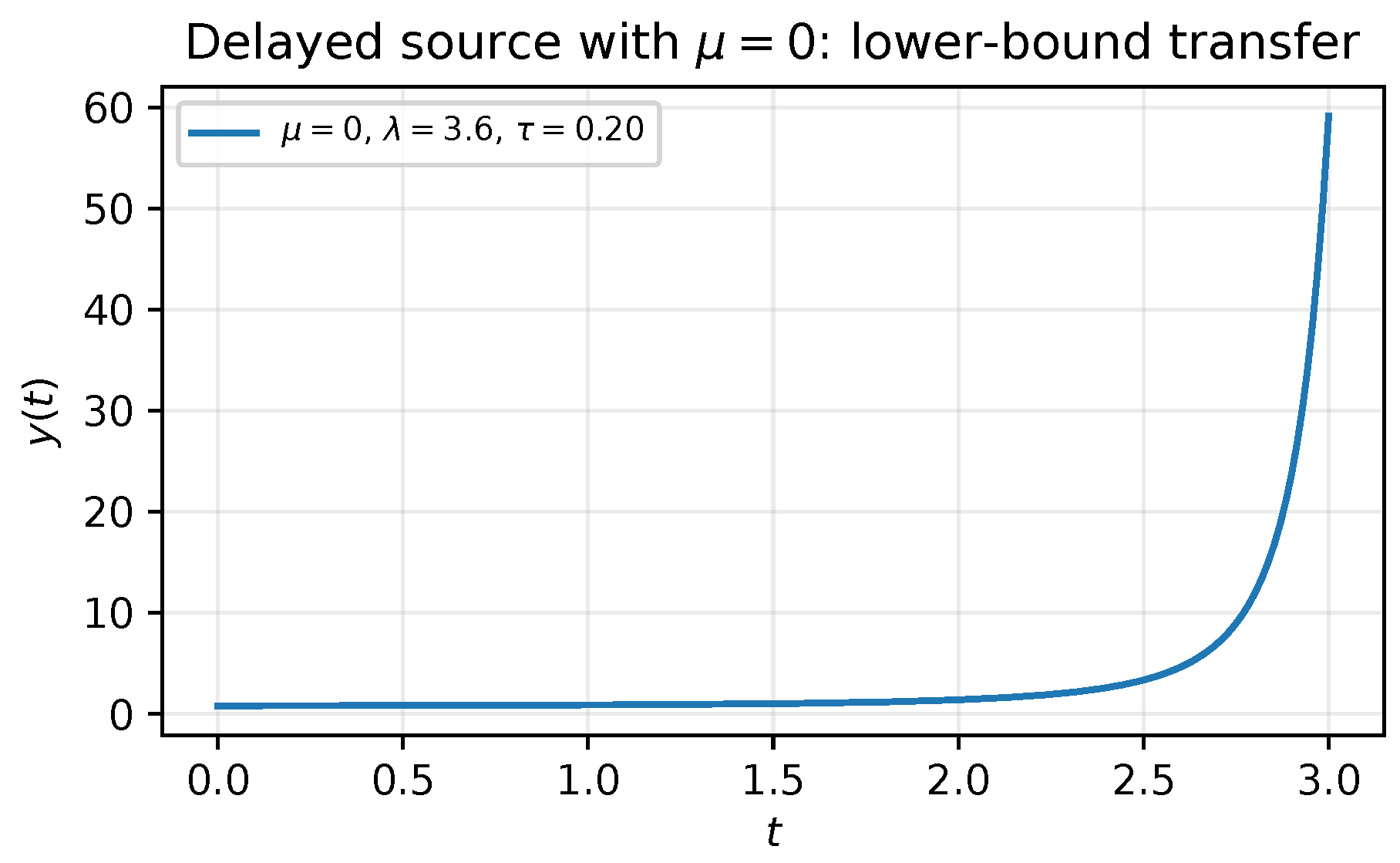
Figure 2 shows delayed lower-bound transfer in the heuristic reduced solution. The increase is generated by values entering through the delayed term, so the transfer becomes visible only after the delayed feedback has returned from the history window.

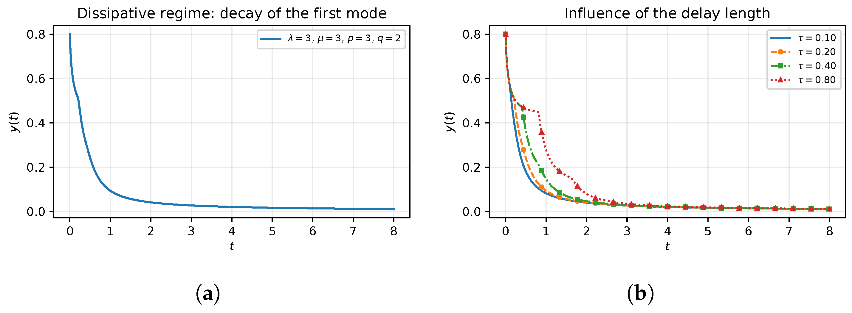
Panel a in Figure 3 illustrates decay under the smallness conditions in the heuristic reduced equation. The delayed input is still present, but it is too small to overcome absorption and spectral damping; the heuristic reduced solution decays toward zero over the computed time interval.

Panel b in Figure 3 illustrates how the length of the delay window changes the transient response. Changing $\tau$ changes when past values re-enter the scalar equation, while the dissipative regime still drives the heuristic reduced solution downward.

These figures accompany the analysis but do not replace it. A space-time discrete approximation of the original PDE would require spectral approximation of $A^s$, treatment of the Caputo derivative and delay, and convergence estimates for the resulting scheme.

9.3. Independent Spatially Resolved Spectral-Galerkin/L1 Computation

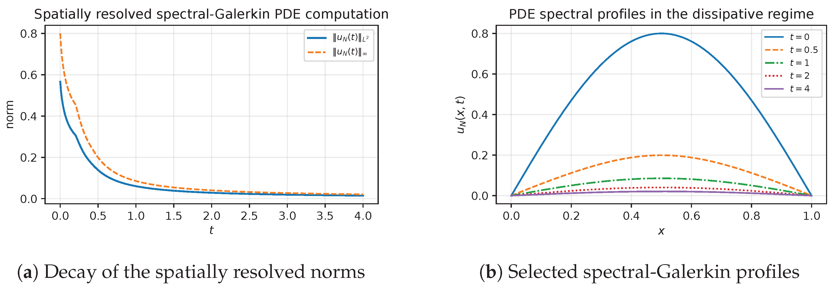
To go beyond the scalar surrogate, we also compute an independent spatially resolved approximation of (8) on $\Omega =(0,1)$. This experiment is not used in the proof and no convergence theorem for the fully discrete nonlinear delay scheme is claimed. Its purpose is to check that the dissipative behavior remains visible when several spatial modes are retained.

Let

$$u_N^n\left(x\right)={\displaystyle \sum _{k=1}^N}{a}_k^n{\varphi }_k\left(x\right),{\varphi }_k\left(x\right)=\sqrt{2}sin\left(k\pi x\right),{\lambda }_k^s={\left(k\pi \right)}^{2s}.$$

For each retained mode, the L1 time formula is combined with

$$D_h^{\alpha }{a}_k^n+{\lambda }_k^s{a}_k^n=\lambda \left({\left(u_{N,\tau }^n\right)}^p,{\varphi }_k\right)-\mu \left({\left(u_N^n\right)}^q,{\varphi }_k\right),1\le k\le N.$$

(31)

The nonlinear projections are evaluated by Gauss–Legendre quadrature. For N retained modes, we use

$$J=\max \{8N,128\}$$

nodes in $(0,1)$. The delay is represented exactly by choosing $\tau /h\in \mathbb{N}$. The present-state absorption is implicit; the resulting N-dimensional system is solved by damped Newton iteration until

$${\displaystyle \frac{\parallel F\left(a^n\right){\parallel }_{\infty }}{\max \{1,\parallel r^n{\parallel }_{\infty }\}}}\le {10}^{-11},$$

where $F\left(a^n\right)=0$ is the nonlinear algebraic system and $r^n$ its right-hand side. At most, 25 Newton iterations are allowed; in the computations below, no step required more than four iterations.

We take

$$\alpha =0.8,s=0.5,\tau =0.2,\lambda =3,\mu =3,p=3,q=2,$$

and the time-independent history

$$\phi (x,t)=0.8sin\left(\pi x\right),-\tau \le t\le 0.$$

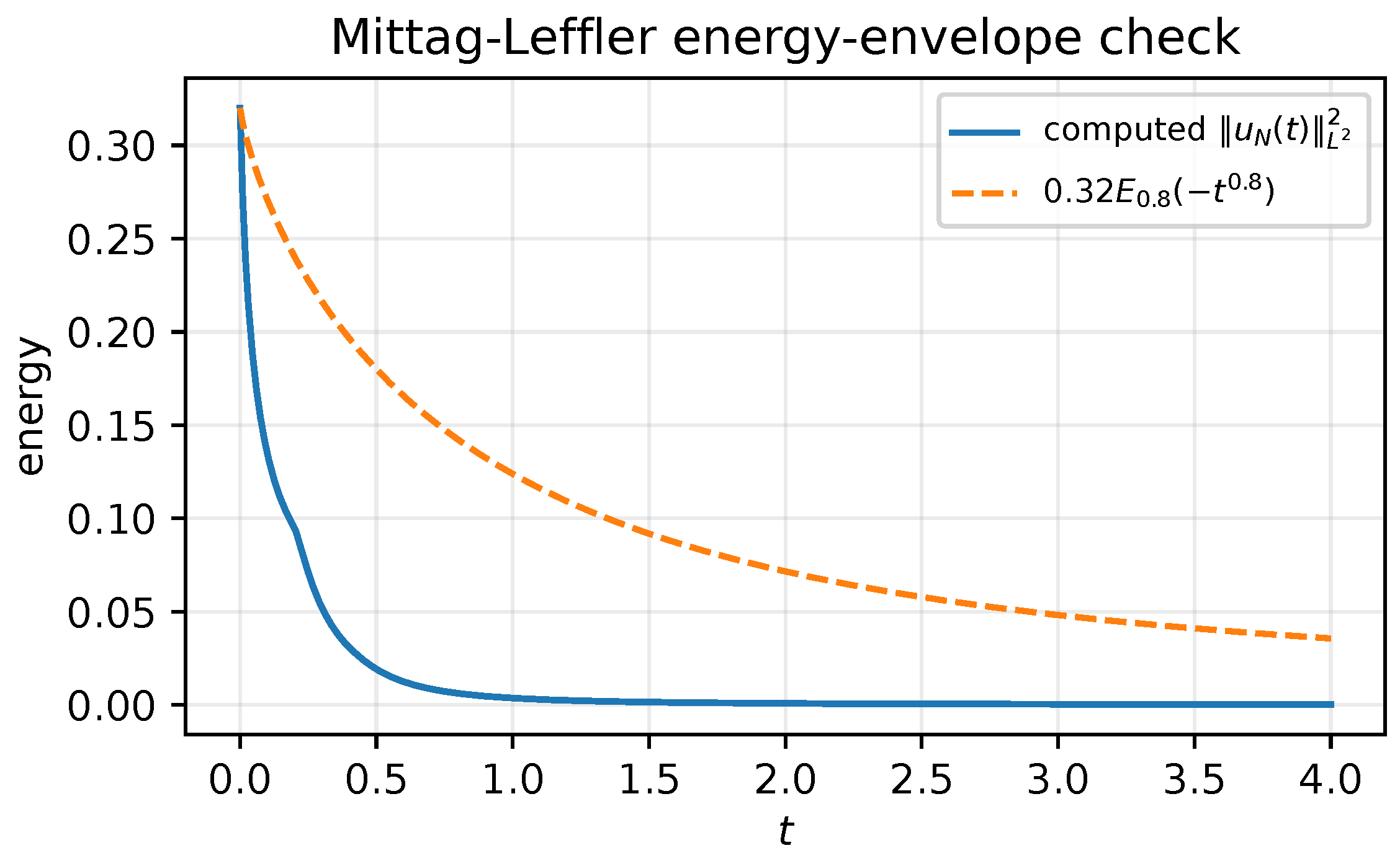
This history satisfies the smallness assumptions of Theorem 3. Figure 4 and Figure 5 use $N=32$, $h=5\times {10}^{-3}$ and $T=4$.

For these parameters,

$${\lambda }_1^s=\pi ,\gamma =2\pi -3{\left(0.8\right)}^2\approx 4.363185,\delta =3{\left(0.8\right)}^2=1.92.$$

Equation (27) gives ${\omega }_{*}\approx 1.461715$, so $\omega =1$ is admissible. Since

$$\underset{-\tau \le \theta \le 0}{sup}{\parallel \phi \left(\theta \right)\parallel }_{L^2(0,1)}^2=0.32,$$

Lemma 6 gives the analytical envelope

$${\parallel u\left(t\right)\parallel }_{L^2(0,1)}^2\le 0.32E_{0.8}(-t^{0.8}).$$

Independent temporal and spectral refinements are reported in

Table 4. Temporal refinement at fixed $N=32$ and spectral-mode refinement at fixed $h={10}^{-2}$ for the spatially resolved PDE computation. The successive discrepancies decrease under both refinements.

Refinement	Resolution	$\parallel {\mathit{u}}_{\mathit{N}}{\mathsf{\left(}4\mathsf{\right)}\parallel }_{{\mathit{L}}^2}$	Successive Error	Max. Newton
Time	$h=2\times {10}^{-2}$	0.01475889	$7.0092\times {10}^{-3}$	4
Time	$h=1\times {10}^{-2}$	0.01473985	$4.1553\times {10}^{-3}$	4
Time	$h=5\times {10}^{-3}$	0.01473054	–	4
Modes	$N=8$	0.01473985	$1.0450\times {10}^{-4}$	4
Modes	$N=16$	0.01473985	$1.1042\times {10}^{-5}$	4
Modes	$N=32$	0.01473985	–	4

. For nested time grids,

$$e_h^{\mathrm{PDE}}=\underset{n}{\max }{\parallel u_{N,h}\left(t_n\right)-u_{N,h/2}\left(t_n\right)\parallel }_{L^2},$$

and, at fixed h,

$$e_N^{\mathrm{PDE}}=\underset{n}{\max }{\parallel u_{N,h}\left(t_n\right)-u_{2N,h}\left(t_n\right)\parallel }_{L^2},$$

where the smaller modal vector is zero-padded before comparison.

The terminal $L^2$-norm stabilizes and the successive-grid discrepancies decrease under both refinements. These data support numerical consistency of the displayed experiment, without replacing a fully discrete convergence analysis.

• Computational reproducibility.

The supplied scripts generate every numerical figure and every CSV table reported in this section from the parameter values stated above. The scripts check that $\tau /h$ is an integer, record the maximum Newton iteration count, and print the Halanay root and the maximum excess of the computed energy over the analytical envelope. Running the scripts from a clean copy of the supplementary directory reproduces the numerical files used in the manuscript.

10. Conclusions

We have studied a Caputo time-fractional semilinear diffusion equation driven by the spectral fractional Dirichlet Laplacian, in which the nonlinear source is delayed while the absorption acts at the present time. The aim was to isolate the delayed first-mode lower-bound transfer estimate and the small-data fractional decay regime, rather than to develop a complete dynamical-system theory. The fractional operators are central in the proof: the Caputo derivative gives the Volterra memory and Mittag–Leffler kernels, whereas the spectral fractional Laplacian provides the energy form and the damping scale ${\lambda }_1^s$.

The first part of the analysis established local existence, positivity and a $C_0(\Omega )$ continuation criterion for bounded nonnegative histories. In the delayed-source case $\mu =0$, the solution can be continued globally, with boundedness on every finite time interval, and the first Dirichlet mode satisfies explicit lower estimates showing how positive lower bounds are transferred from one delay interval to the next. This delayed transfer is a stepwise lower-bound propagation, not a finite-time blow-up result.

In the dissipative case $\mu >0$, the smallness assumptions

$$\lambda {\epsilon }^{p-q}\le \mu ,\lambda {\epsilon }^{p-1}<{\lambda }_1^s$$

ensure that small histories remain trapped below the barrier $0\le u\le \epsilon$. The absorption term is used to obtain this invariant barrier, and under the barrier the delayed source is small enough to be dominated by the spectral damping in the energy estimate. This yields global boundedness and convergence to zero in $L^2(\Omega )$, with a Mittag–Leffler-type estimate for the $L^2$-energy. This decay statement is fractional in nature: it replaces the exponential energy scale of the classical parabolic case by the Mittag–Leffler scale associated with the Caputo derivative.

The numerical section separates two levels of computation. The scalar equations remain explicitly heuristic first-mode surrogates and carry no PDE comparison claim in the dissipative case. Independently, a spatially resolved sine spectral-Galerkin/L1 computation of the original one-dimensional PDE was performed with temporal and mode refinements and a direct Mittag–Leffler envelope check. The computed norms and profiles decay, the reported energy remains below the stated Mittag–Leffler envelope on the computed grid, and the successive refinement discrepancies decrease. These observations do not substitute for a fully discrete convergence theorem.

• Preprint disclosure

An earlier, non-peer-reviewed version of this work was posted on Preprints.org on 16 July 2026 as Version 1, https://doi.org/10.20944/preprints202607.1183.v1, (accessed on 2 August 2026). The present revised manuscript substantially changes that version, including the phase space, weak Caputo and truncation framework, continuation and Halanay arguments, and numerical scope. The preprint is disclosed as an earlier version and is not used as evidence for any result proved here.

References

1. Kaplan, S. On the growth of solutions of quasi-linear parabolic equations. Commun. Pure Appl. Math. 1963, 16, 305–330. [Google Scholar] [CrossRef] [Scilit]
2. Fujita, H. On the blowing up of solutions of the Cauchy problem for ut = Δu + u1+α. J. Fac. Sci. Univ. Tokyo Sect. I 1966, 13, 109–124. [Google Scholar] [CrossRef]
3. Henry, D. Geometric Theory of Semilinear Parabolic Equations; Lecture Notes in Mathematics; Springer: Berlin, Germany, 1981; Volume 840. [Google Scholar]
4. Pazy, A. Semigroups of Linear Operators and Applications to Partial Differential Equations; Applied Mathematical Sciences; Springer: New York, NY, USA, 1983; Volume 44. [Google Scholar]
5. Quittner, P.; Souplet, P. Superlinear Parabolic Problems: Blow-up, Global Existence and Steady States; Birkhäuser: Basel, Switzerland, 2007. [Google Scholar]
6. Podlubny, I. Fractional Differential Equations; Academic Press: San Diego, CA, USA, 1999. [Google Scholar]
7. Kilbas, A.A.; Srivastava, H.M.; Trujillo, J.J. Theory and Applications of Fractional Differential Equations; Elsevier: Amsterdam, The Netherlands, 2006. [Google Scholar]
8. Diethelm, K. The Analysis of Fractional Differential Equations; Lecture Notes in Mathematics; Springer: Berlin, Germany, 2010; Volume 2004. [Google Scholar]
9. Gorenflo, R.; Kilbas, A.A.; Mainardi, F.; Rogosin, S.V. Mittag-Leffler Functions, Related Topics and Applications; Springer: Berlin, Germany, 2014. [Google Scholar] [CrossRef] [Scilit]
10. Luchko, Y. Maximum principle for the generalized time-fractional diffusion equation. J. Math. Anal. Appl. 2009, 351, 218–223. [Google Scholar] [CrossRef] [Scilit]
11. Luchko, Y. Maximum principle and its application for the time-fractional diffusion equations. Fract. Calc. Appl. Anal. 2011, 14, 110–124. [Google Scholar] [CrossRef] [Scilit]
12. Sakamoto, K.; Yamamoto, M. Initial value/boundary value problems for fractional diffusion-wave equations and applications to some inverse problems. J. Math. Anal. Appl. 2011, 382, 426–447. [Google Scholar] [CrossRef] [Scilit]
13. Caffarelli, L.; Silvestre, L. An extension problem related to the fractional Laplacian. Commun. Partial Differ. Equ. 2007, 32, 1245–1260. [Google Scholar] [CrossRef] [Scilit]
14. Di Nezza, E.; Palatucci, G.; Valdinoci, E. Hitchhiker’s guide to the fractional Sobolev spaces. Bull. Sci. Math. 2012, 136, 521–573. [Google Scholar] [CrossRef] [Scilit]
15. Servadei, R.; Valdinoci, E. Variational methods for non-local operators of elliptic type. Discrete Contin. Dyn. Syst. 2013, 33, 2105–2137. [Google Scholar] [CrossRef] [Scilit]
16. Stinga, P.R.; Torrea, J.L. Extension problem and Harnack’s inequality for some fractional operators. Commun. Partial Differ. Equ. 2010, 35, 2092–2122. [Google Scholar] [CrossRef] [Scilit]
17. Bonito, A.; Pasciak, J.E. Numerical approximation of fractional powers of elliptic operators. Math. Comput. 2015, 84, 2083–2110. [Google Scholar] [CrossRef] [Scilit]
18. Shi, L.; Cheng, W.; Mao, J.; Xu, T. Blow-up and global existence of solutions for the time fractional reaction–diffusion equation. Mathematics 2021, 9, 3248. [Google Scholar] [CrossRef] [Scilit]
19. Aldawish, I.; Samet, B. On the critical behavior for time-fractional reaction diffusion problems. Discrete Contin. Dyn. Syst. 2023, 16, 2015–2032. [Google Scholar] [CrossRef] [Scilit]
20. Igarashi, T. The second critical exponent for a time-fractional reaction-diffusion equation. Mathematics 2024, 12, 2895. [Google Scholar] [CrossRef] [Scilit]
21. Jabbarkhanov, K.; Suragan, D. Dynamics of nonlinear anomalous reaction-diffusion models: Global existence and blow-up of solutions. Evol. Equ. Control Theory 2025, 14, 1128–1140. [Google Scholar] [CrossRef] [Scilit]
22. Zhang, Q.; Ren, Y.; Lin, X.; Xu, Y. Uniform convergence of compact and BDF methods for the space fractional semilinear delay reaction–diffusion equations. Appl. Math. Comput. 2019, 358, 91–110. [Google Scholar] [CrossRef] [Scilit]
23. Jian, H.-Y.; Huang, T.-Z.; Ostermann, A.; Gu, X.-M.; Zhao, Y.-L. Fast numerical schemes for nonlinear space-fractional multidelay reaction–diffusion equations by implicit integration factor methods. Appl. Math. Comput. 2021, 408, 126360. [Google Scholar] [CrossRef] [Scilit]
24. Halanay, A. Differential Equations: Stability, Oscillations, Time Lags; Academic Press: New York, NY, USA, 1966. [Google Scholar]
25. Hale, J.K.; Verduyn Lunel, S.M. Introduction to Functional Differential Equations; Applied Mathematical Sciences; Springer: New York, NY, USA, 1993; Volume 99. [Google Scholar]
26. Gripenberg, G.; Londen, S.-O.; Staffans, O. Volterra Integral and Functional Equations; Cambridge University Press: Cambridge, UK, 1990. [Google Scholar]
27. Hendy, A.S.; Zaky, M.A.; Van Bockstal, K. Theoretical and numerical aspects for the long-time behavior of nonlinear delay time Caputo fractional reaction-diffusion equations. Nonlinear Dyn. 2023, 111, 3525–3537. [Google Scholar] [CrossRef] [Scilit]
28. Thinh, L.V.; Tuan, H.T. A generalized fractional Halanay inequality and its applications. SIAM J. Control Optim. 2025, 63, 916–935. [Google Scholar] [CrossRef] [Scilit]
29. Zacher, R. Weak solutions of abstract evolutionary integro-differential equations in Hilbert spaces. Funkcial. Ekvacioj 2009, 52, 1–18. [Google Scholar] [CrossRef] [Scilit]
30. Zacher, R. A De Giorgi–Nash type theorem for time fractional diffusion equations. Math. Ann. 2013, 356, 99–146. [Google Scholar] [CrossRef] [Scilit]
31. Vergara, V.; Zacher, R. Optimal decay estimates for time-fractional and other nonlocal subdiffusion equations via energy methods. SIAM J. Math. Anal. 2015, 47, 210–239. [Google Scholar] [CrossRef] [Scilit]
32. Fukushima, M.; Oshima, Y.; Takeda, M. Dirichlet Forms and Symmetric Markov Processes, 2nd ed.; De Gruyter Studies in Mathematics; Walter de Gruyter: Berlin, Germany, 2011; Volume 19. [Google Scholar]
33. Ouhabaz, E.M. Analysis of Heat Equations on Domains; London Mathematical Society Monographs Series; Princeton University Press: Princeton, NJ, USA, 2005; Volume 31. [Google Scholar]
34. Lin, Y.; Xu, C. Finite difference/spectral approximations for the time-fractional diffusion equation. J. Comput. Phys. 2007, 225, 1533–1552. [Google Scholar] [CrossRef] [Scilit]
Figure 1. Schematic distinction between the distributed Volterra memory generated by the Caputo derivative and the discrete feedback generated by the strict delay.
Appliedmath 06 00135 g001
Figure 2. Heuristic reduced model: delayed lower-bound transfer in the delayed-source regime with μ = 0 .
Appliedmath 06 00135 g002
Figure 3. Heuristic reduced illustrations in the dissipative regime. (a) Decay of the heuristic reduced solution. (b) Delay-length effect in the heuristic reduced model on the transient response while the dissipative regime still drives the solution toward zero. The curves in panel (b) are distinguished by color, line style, and markers. (a) Decay under the smallness conditions. (b) Delay-length effect in the heuristic reduced model.
Appliedmath 06 00135 g003
Figure 4. Independent spatially resolved spectral-Galerkin/L1 computation of the delayed PDE in the dissipative regime. The norm histories and the selected profiles decay while preserving the homogeneous Dirichlet boundary behavior. This is not a scalar first-mode comparison.
Appliedmath 06 00135 g004
Figure 5. Computed spectral-Galerkin energy and the admissible analytical Mittag–Leffler envelope 0.32 E 0.8 ( t 0.8 ) . The computed energy remains below the envelope on the reported grid; this is a consistency check, not a numerical proof of Theorem 3.
Appliedmath 06 00135 g005