Article

Mathematical Modeling and Analysis of Atmospheric Carbon Dioxide (CO2) Dynamics with Human Population Growth and Vehicle Services Age


by
Ashenafi Kelemu Mengistu
1,
Elias Merkebu Adamu
1,
Getachew Tilahun Affesa
1,
Yeshambel Azene Belay
1 and
Peter Joseph Witbooi
2,*
1
Department of Mathematics, Woldia University, Woldia P.O. Box 400, Ethiopia
2
Department of Mathematics and Applied Mathematics, University of the Western Cape, Private Bag X17, Cape Town 7535, South Africa
*
Author to whom correspondence should be addressed.
AppliedMath 2026, 6(8), 122; https://doi.org/10.3390/appliedmath6080122
Submission received: 4 June 2026 / Revised: 25 June 2026 / Accepted: 1 July 2026 / Published: 27 July 2026
(This article belongs to the Section Computational and Numerical Mathematics)

Abstract

In this study, we propose a mathematical model for the dynamics of atmospheric carbon dioxide (CO2) with human population growth and an age-structured vehicle population. The positivity and boundedness of the model’s solutions are verified, and the global stability of an interior equilibrium point is proved. We calibrate the model parameters using the least-squares method. Simulations of the model show good alignment with the reported atmospheric CO2 data. Moreover, the sensitivity analysis shows that human-related emission factors and emissions from old vehicles are the main contributors to CO2 accumulation. The results of this study recommend that reducing anthropogenic emissions, accelerating the retirement of old vehicles, and strengthening carbon sequestration initiatives be considered to mitigate future atmospheric CO2 accumulation.

1. Introduction

The rapid escalation of atmospheric carbon dioxide (CO2) over recent decades has emerged as the defining crisis of the modern era. The continuous accumulation of atmospheric CO2 acts as the primary driver of global climate change, yielding profound and long-lasting adverse impacts on environmental stability, weather patterns, air quality, and public health [1,2,3]. This crisis is largely driven by human activities, including industrial expansion, fossil fuel combustion for energy production, large-scale deforestation, growing transportation demands, and intensive agricultural practices that weaken the Earth’s natural capacity to absorb carbon [4,5,6]. Among the various sectors contributing to CO2 emissions, transportation is widely recognized as one of the largest and fastest-growing sources worldwide [7,8,9]. In particular, the transport sector accounts for approximately 15% of total anthropogenic greenhouse gas emissions and around 23% of all energy-related greenhouse gas releases globally [10].
Vehicle fleet characteristics such as service age, total mileage, and mechanical condition significantly influence CO2 emission levels. Data from fleet-tracking systems highlight substantial variations in emissions related to vehicle deterioration over time. Korzeb et al. [11] demonstrated that vehicles with cumulative mileage up to 86,000 km emit substantially less CO2 than those operating between 86,001 and 160,000 km. Correspondingly, Singam et al. [12] identified vehicle age, baseline fuel consumption, driving habits, and maintenance frequency as critical determinants affecting emissions. These observations are corroborated by engineering analyses and data-driven models, which reveal that component wear degrades engine combustion efficiency, thereby elevating carbon emissions [13].
In response to the growing concern over atmospheric CO2 accumulation, various mathematical models have been developed to examine how socioeconomic, technological, and environmental factors govern CO2 dynamics [5,14,15,16,17,18,19]. For instance, Misra et al. [14] proposed a compartment model that examined the relationship between atmospheric CO2 accumulation and mitigation budget allocations, finding that rising CO2 levels directly increase funding requirements for mitigation efforts. On the ecological side, Sundar et al. [15] showed that targeted green belt development and seaweed farming can substantially reduce ambient carbon levels by enhancing photosynthetic absorption near major urban emission sources. Addressing demographic drivers, Fors [16] developed a mathematical model demonstrating that human population growth accelerates deforestation, which in turn raises the equilibrium concentration of atmospheric CO2. Additionally, nonlinear dynamic models have been used to assess carbon fluctuations under varying plant absorption capacities [19], as well as the feedback relationships between reforestation efforts and human population pressures [17,18].
Most existing mathematical models focus on broad interactions among human populations, industrial activities, and atmospheric CO2 concentrations. Even when vehicular activity is explicitly incorporated, vehicles are often assumed to emit CO2 at the same constant rate, regardless of their service age or condition. For example, Mehmood et al. [20] developed a model to investigate the effects of emissions from fossil-fueled vehicles on atmospheric CO2 concentrations and global warming. However, their study assumed identical CO2 emission rates for all vehicles and did not account for differences in emissions due to variations in vehicle age and condition.
Donald et al. [5] developed a nonlinear compartmental model to investigate the contribution of vehicular activities to atmospheric CO2 accumulation. The model incorporated human population, vehicle population, forest biomass, and atmospheric carbon dioxide as interacting compartments. The authors analyzed the existence and stability of equilibrium points and estimated model parameters using available data. Sensitivity analysis and numerical simulations were also conducted to assess the influence of various parameters on CO2 dynamics. The study demonstrated that increasing vehicular activities significantly elevates atmospheric CO2 concentrations. However, the model assumed that all vehicles emit CO2 at the same rate, without considering differences arising from vehicle age or condition. This limitation provides an opportunity for extending the model by incorporating age-structured vehicle classes.
Liu et al. [21] employed a system dynamics approach to evaluate the impact of transportation policies on carbon dioxide emissions. The study simulated the effects of measures such as improving public transportation, implementing vehicle restrictions, and promoting fuel efficiency. Their findings suggested that integrated transport policies can substantially reduce future emissions. However, the analysis focused primarily on policy scenarios and simulation outcomes without conducting rigorous mathematical investigations such as equilibrium analysis or stability assessment.
Chang et al. [22] proposed a real-time emission estimation framework using intelligent transportation system technologies. The model incorporated traffic characteristics such as vehicle speed, acceleration, and road conditions to estimate CO2 emissions more accurately. The study demonstrated the usefulness of traffic monitoring systems for managing urban emissions and improving transport efficiency. Despite its practical significance, the work focused on short-term emission estimation and did not address the long-term dynamics of atmospheric CO2 accumulation.
Cardona et al. [23] developed a system dynamics model to estimate and project CO2 emissions from the transport sector under different development scenarios. The study assessed the long-term implications of transportation growth and explored strategies for emission mitigation. The results emphasized the importance of sustainable transport planning in controlling emissions. Nevertheless, the model did not explicitly describe atmospheric CO2 accumulation mechanisms and lacked an analytical examination of the system’s dynamic properties.
Overall, these studies demonstrate substantial progress in modeling carbon dioxide dynamics and transportation-related emissions. However, they reveal important research gaps, particularly the absence of age-structured vehicle populations and the limited integration of transportation dynamics with rigorous mathematical analysis of atmospheric CO2 accumulation. These gaps motivate the development of models that account for heterogeneous vehicle fleets and provide a deeper understanding of the long-term impacts of transportation on climate change.

2. Model Formulation

In this study, we develop a deterministic compartmental mathematical model to describe the dynamics of atmospheric CO2 concentration influenced by human population growth, vehicle fleet expansion, and human activities. The model consists of five interacting state variables: the human population, H ( t ) ; three vehicle age classes, V 1 ( t ) , V 2 ( t ) , and V 3 ( t ) ; and the accumulated atmospheric CO2 concentration, C ( t ) .
Human population dynamics: Although the logistic growth model has some limitations, such as assuming a homogeneous population and neglecting socioeconomic, cultural, and policy factors, it has been widely used to describe human population growth [24,25,26]. Therefore, for simplicity and consistency with previous studies, we assume that the human population follows logistic growth.
Let H ( t ) denote the human population at time t. The population grows at an intrinsic rate s, while environmental limitations restrict its growth through the carrying capacity K. Under these assumptions, the human population dynamics are given by
d H d t = s H 1 H K .
Human population dynamics play an important role in the model because vehicle ownership and other human activities depend on population size. We assume that new vehicles enter the system at a rate proportional to the human population, given by Λ H , where Λ is the per capita vehicle acquisition rate.
Vehicle fleet dynamics: The vehicle fleet is divided into three groups according to vehicle age and cumulative mileage. Based on fleet distribution data reported in [27,28,29], the vehicle classes are defined as follows:
  • V 1 ( t ) represents new vehicles with less than three years of service and cumulative mileage below 30,000 miles.
  • V 2 ( t ) represents mid-aged vehicles with 3–6 years of service and mileage between 30,000 and 100,000 miles.
  • V 3 ( t ) represents old vehicles with more than seven years of service and mileage exceeding 100,000 miles.
Vehicles are assumed to move sequentially through these classes as they age and accumulate mileage. New vehicles progress to the mid-aged class at rate α 1 , while mid-aged vehicles move to the old vehicle class at rate α 2 . Vehicles may also leave each class because of retirement, scrappage, or mechanical failure. These removals occur at rates μ 1 , μ 2 , and μ 3 , respectively.
An important assumption of the model is that older vehicles emit more CO2 due to reduced engine efficiency and technological deterioration. Consequently, the emission rates satisfy
β 1 < β 2 < β 3 ,
where β i represents the CO2 emission rate of the i-th vehicle class. The vehicle population dynamics are therefore given by
d V 1 d t = Λ H ( α 1 + μ 1 ) V 1 , d V 2 d t = α 1 V 1 ( α 2 + μ 2 ) V 2 , d V 3 d t = α 2 V 2 μ 3 V 3 .
Atmospheric CO2 dynamics: The final component of the model describes the accumulated atmospheric carbon dioxide concentration, denoted by C ( t ) . Atmospheric CO2 accumulates from three main sources:
  • Natural processes and biological respiration contribute CO2 at a constant rate δ .
  • Human activities, including energy consumption, industrial production, and land-use changes, contribute CO2 at a rate proportional to the population size, given by θ H .
  • Vehicular emissions arise from the three vehicle classes and are represented by
    β 1 V 1 + β 2 V 2 + β 3 V 3 .
To capture the major mechanisms of the carbon cycle, the model incorporates two pathways for CO2 removal. The first pathway represents natural sequestration through forests, soils, and oceans, occurring at rate γ 1 C . The second pathway represents human mitigation efforts, such as carbon capture technologies and reforestation programs, occurring at rate γ 2 C . Therefore, the atmospheric CO2 dynamics are described by
dC dt = δ + θ H + β 1 V 1 + β 2 V 2 + β 3 V 3 ( γ 1 + γ 2 ) C .
Combining the above components, we obtain the following system of nonlinear differential equations:
dH dt = sH 1 H K , dV 1 dt = Λ H ( α 1 + μ 1 ) V 1 , dV 2 dt = α 1 V 1 ( α 2 + μ 2 ) V 2 , dV 3 dt = α 2 V 2 μ 3 V 3 , dC dt = δ + θ H + β 1 V 1 + β 2 V 2 + β 3 V 3 ( γ 1 + γ 2 ) C ,
where the initial data
H ( 0 ) 0 , V 1 ( 0 ) 0 , V 2 ( 0 ) 0 , V 3 ( 0 ) 0 , C ( 0 ) 0 .
To ensure biological, physical, and environmental realism, all model parameters are assumed to be positive. The definitions of the state variables and model parameters are presented in Table 1 and Table 2, respectively.

3. Qualitative Analysis

3.1. Positivity and Boundedness of a Solution

Since the proposed model describes the dynamics of the human population, vehicle fleets, and atmospheric CO2 concentration, it is necessary to ensure that all state variables remain non-negative for all time t > 0 . This requirement guarantees the biological and physical feasibility of the model.
In this section, we establish two fundamental properties of system (1): positivity and boundedness of the solutions.
Theorem 1 Positivity of Solutions).
(Consider the system (1) with strictly positive parameters and initial conditions
H ( 0 ) > 0 , V 1 ( 0 ) > 0 , V 2 ( 0 ) > 0 , V 3 ( 0 ) > 0 , C ( 0 ) > 0 .
Then, the solutions
H ( t ) , V 1 ( t ) , V 2 ( t ) , V 3 ( t ) , C ( t )
remain strictly positive for all t 0 .
Proof. 
The first equation of the system (1) is a differential equation of the logistic form:
dH dt = sH 1 H K .
The solution for H ( t ) is given by
H ( t ) = KH ( 0 ) e st K + H ( 0 ) ( e st 1 ) .
Given that s > 0 and H ( 0 ) > 0 , the exponential nature of the solution ensures that H ( t ) > 0 for all t 0 .
To establish the positivity of V 1 ( t ) , we consider the second equation of system (1):
dV 1 dt = Λ H ( α 1 + μ 1 ) V 1 .
Using the integrating factor e ( α 1 + μ 1 ) t , the general solution is
V 1 ( t ) = e ( α 1 + μ 1 ) t V 1 ( 0 ) + Λ 0 t H ( τ ) e ( α 1 + μ 1 ) τ d τ .
Given that H ( τ ) > 0 , all terms on the right-hand side are positive. Consequently, V 1 ( t ) > 0 for all t 0 .
Similarly, for the mid-aged vehicle cohort:
dV 2 dt = α 1 V 1 ( α 2 + μ 2 ) V 2 ,
using the integrating factor e ( α 2 + μ 2 ) t the general solution is
V 2 ( t ) = e ( α 2 + μ 2 ) t V 2 ( 0 ) + α 1 0 t V 1 ( τ ) e ( α 2 + μ 2 ) τ d τ .
Since V 1 ( τ ) > 0 , it follows that V 2 ( t ) > 0 for all t 0 .
For the old vehicle cohort V 3 :
dV 3 dt = α 2 V 2 μ 3 V 3 ,
and using the integrating factor e μ 3 t , the general solution is
V 3 ( t ) = e μ 3 t V 3 ( 0 ) + α 2 0 t V 2 ( τ ) e μ 3 τ d τ .
Since V 2 ( τ ) > 0 , we obtain V 3 ( t ) > 0 for all t 0 .
Finally, we consider the equation of atmospheric CO2 concentration C ( t ) :
dC dt = δ + θ H + β 1 V 1 + β 2 V 2 + β 3 V 3 ( γ 1 + γ 2 ) C .
Using the integrating factor e ( γ 1 + γ 2 ) t , we have:
C ( t ) = e ( γ 1 + γ 2 ) t C ( 0 ) + 0 t δ + θ H + β 1 V 1 + β 2 V 2 + β 3 V 3 e ( γ 1 + γ 2 ) τ d τ .
Because all parameters and state variables are positive, the integrand is positive, ensuring C ( t ) > 0 for all t 0 . Therefore, each state variable remains strictly positive for all t 0 whenever the initial data are strictly positive. This proves that the region R + 5 is positively invariant for system (1). □
Theorem 2 (Boundedness of Solutions).
Consider the system (1) with strictly positive parameters and non-negative initial conditions in R + 5 . Then all solutions of the system remain bounded for all t > 0 . Moreover, there exists a positively invariant bounded region
Ω = ( H , V 1 , V 2 , V 3 , C ) R + 5 : H K , V 1 M 1 , V 2 M 2 , V 3 M 3 , C M 4 ,
which attracts all the trajectories.
Proof. 
Since the right-hand side of the system (1) is locally Lipschitz in R + 5 , solutions exist and are unique for all t > 0 . From the first equation of the system (1):
dH dt = sH 1 H K
which is a standard logistic equation. This implies the following:
0 H ( t ) max { H ( 0 ) , K } , for all t > 0 .
In particular, if H ( 0 ) K , then 0 H ( t ) K for all t > 0 , ensuring H ( t ) is uniformly bounded. Next, consider the dynamics of the new vehicle cohort V 1 ( t ) :
dV 1 dt = Λ H ( α 1 + μ 1 ) V 1 .
Given H ( t ) K , we obtain
dV 1 dt Λ K ( α 1 + μ 1 ) V 1 .
By the comparison theorem, it follows that
0 V 1 ( t ) max V 1 ( 0 ) , Λ K α 1 + μ 1 = M 1 , for all t > 0 .
For the mid-aged vehicle cohort V 2 ( t ) :
dV 2 dt = α 1 V 1 ( α 2 + μ 2 ) V 2 .
The boundedness of V 1 ( t ) implies
dV 2 dt α 1 M 1 ( α 2 + μ 2 ) V 2 .
Applying the comparison theorem again yields
0 V 2 ( t ) max V 2 ( 0 ) , α 1 M 1 α 2 + μ 2 = M 2 , for all t > 0 .
For the old vehicle cohort V 3 ( t ) :
dV 3 dt = α 2 V 2 μ 3 V 3 .
Using the boundedness of V 2 ( t ) , we obtain
dV 3 dt α 2 M 2 μ 3 V 3 .
By comparison, it follows that
0 V 3 ( t ) max V 3 ( 0 ) , α 2 M 2 μ 3 = M 3 , for all t > 0 .
Finally, consider the carbon concentration equation
dC dt = δ + θ H + β 1 V 1 + β 2 V 2 + β 3 V 3 ( γ 1 + γ 2 ) C .
Since V 1 ( t ) , V 2 ( t ) , and V 3 ( t ) are bounded, let
M = δ + θ K + β 1 M 1 + β 2 M 2 + β 3 M 3 .
Thus,
dC dt M ( γ 1 + γ 2 ) C .
By the comparison theorem,
0 C ( t ) max C ( 0 ) , M γ 1 + γ 2 = M 4 , for all t > 0 .
Hence, all solution sets of the system (1) remain bounded for all t > 0 . Consequently, there exists a positively invariant compact region Ω R + 5 that attracts all the trajectories of the system (1). □

3.2. Equilibrium Points of the System

Equilibrium points of the system (1) correspond to steady states where all state variables remain constant over time. These points are obtained by setting the right-hand sides of the system to zero. That is, an equilibrium point
( H * , V 1 * , V 2 * , V 3 * , C * )
satisfies
dH / dt = ( dV 1 ) / dt = ( dV 2 ) / dt = ( dV 3 ) / dt = dC / dt = 0 .
Using system (1), the equilibrium conditions are therefore given by
0 = sH * 1 H * K 0 = Λ H * ( α 1 + μ 1 ) V 1 * 0 = α 1 V 1 * ( α 2 + μ 2 ) V 2 * 0 = α 2 V 2 * μ 3 V 3 * 0 = δ + θ H * + β 1 V 1 * + β 2 V 2 * + β 3 V 3 * ( γ 1 + γ 2 ) C *
The first equation satisfies either
H * = 0
or
H * = K .
Thus, system (1) admits two equilibrium points.
If
H * = 0 ,
V 1 * = V 2 * = V 3 * = 0 ,
and
C * = δ γ 1 + γ 2 .
Thus, the system admits the boundary equilibrium
E 0 * = 0 , 0 , 0 , 0 , δ γ 1 + γ 2 .
This equilibrium corresponds to a hypothetical scenario in which no human population and no vehicles exist, and the atmospheric CO2 concentration is determined solely by natural processes and environmental sequestration.
If
H * = K ,
we obtain the interior equilibrium
E 1 * = ( H * , V 1 * , V 2 * , V 3 * , C * ) ,
where
H * = K , V 1 * = K Λ α 1 + μ 1 , V 2 * = K Λ α 1 ( α 1 + μ 1 ) ( α 2 + μ 2 ) , V 3 * = K Λ α 1 α 2 ( α 1 + μ 1 ) ( α 2 + μ 2 ) μ 3 , and C * = β 1 V 1 * + β 2 V 2 * + β 3 V 3 * + δ + K θ γ 1 + γ 2 .
Since all parameters are positive, the interior equilibrium E 1 * is strictly positive and biologically feasible.

3.3. Local Stability Analysis of the Equilibrium Points

To analyze the local stability of the equilibrium points, we first compute the Jacobian matrix of system (1).
Let
E = ( H , V 1 , V 2 , V 3 , C ) ,
then Jacobian matrix J ( E ) of system (1) is
J ( E ) = s ( 1 2 H / K ) 0 0 0 0 Λ α 1 μ 1 0 0 0 0 α 1 α 2 μ 2 0 0 0 0 α 2 μ 3 0 θ β 1 β 2 β 3 γ 1 γ 2 .
Local Stability of the boundary equilibrium point E 0 * :
To investigate the local stability of the boundary equilibrium point E 0 * , the Jacobian matrix is evaluated at this point, yielding
J ( E 0 * ) = s 0 0 0 0 Λ α 1 μ 1 0 0 0 0 α 1 α 2 μ 2 0 0 0 0 α 2 μ 3 0 θ β 1 β 2 β 3 γ 1 γ 2 .
Since the matrix is lower triangular, its eigenvalues are given by the diagonal entries:
λ 1 = s , λ 2 = ( γ 1 + γ 2 ) , λ 3 = ( α 1 + μ 1 ) , λ 4 = ( α 2 + μ 2 ) , λ 5 = μ 3 .
Since s > 0 , one eigenvalue is positive. Therefore, the equilibrium point E 0 * is unstable.
Theorem 3.
The boundary equilibrium point E 0 * of system (1) is unstable.
This result indicates that a system with no human population and no vehicles cannot persist. Any small introduction of population will cause the system to move away from E 0 * .
Local Stability of the Interior Equilibrium E 1 * : Evaluating the Jacobian matrix at E 1 * gives
J ( E 1 * ) = s 0 0 0 0 Λ α 1 μ 1 0 0 0 0 α 1 α 2 μ 2 0 0 0 0 α 2 μ 3 0 θ β 1 β 2 β 3 γ 1 γ 2 .
The eigenvalues of this matrix are
λ 1 = s , λ 2 = ( γ 1 + γ 2 ) , λ 3 = ( α 1 + μ 1 ) , λ 4 = ( α 2 + μ 2 ) , λ 5 = μ 3 .
Since all parameters are positive, all eigenvalues are negative. Thus we have proved the following.
Theorem 4.
The interior equilibrium point E 1 * of system (1) is locally asymptotically stable within the invariant region Ω.

4. Global Stability Analysis

Theorem 5.
The interior equilibrium point E 1 * of system (1) is globally asymptotically stable in the invariant region Ω.
Proof. 
First, consider the human population equation
dH dt = sH 1 H K .
The logistic equation admits the explicit solution
H ( t ) = KH 0 H 0 + ( K H 0 ) e st ,
where H 0 = H ( 0 ) > 0 . Consequently,
lim t H ( t ) = K .
Since the interior equilibrium satisfies
H * = K ,
it follows that
lim t H ( t ) H * = 0 .
Next, define the error variable
e 1 ( t ) = V 1 ( t ) V 1 * .
Using the equation
dV 1 dt = Λ H ( α 1 + μ 1 ) V 1 ,
together with the equilibrium relation
0 = Λ H * ( α 1 + μ 1 ) V 1 * ,
we obtain
e ˙ 1 = Λ ( H H * ) ( α 1 + μ 1 ) e 1 .
Applying the variation-of-constants formula yields
e 1 ( t ) = e ( α 1 + μ 1 ) t e 1 ( 0 ) + Λ 0 t e ( α 1 + μ 1 ) ( t τ ) H ( τ ) H * d τ .
Since α 1 + μ 1 > 0 and
H ( t ) H * 0 as t ,
the first term converges to zero exponentially, while the integral term also tends to zero. Therefore,
lim t e 1 ( t ) = 0 ,
which implies
lim t V 1 ( t ) = V 1 * .
Similarly, define
e 2 ( t ) = V 2 ( t ) V 2 * .
Using
dV 2 dt = α 1 V 1 ( α 2 + μ 2 ) V 2
and the equilibrium identity
0 = α 1 V 1 * ( α 2 + μ 2 ) V 2 * ,
we obtain
e ˙ 2 = α 1 e 1 ( α 2 + μ 2 ) e 2 .
Applying the variation-of-constants formula gives
e 2 ( t ) = e ( α 2 + μ 2 ) t e 2 ( 0 ) + α 1 0 t e ( α 2 + μ 2 ) ( t τ ) e 1 ( τ ) d τ .
Since α 2 + μ 2 > 0 and e 1 ( t ) 0 , it follows that
lim t e 2 ( t ) = 0 .
Hence,
lim t V 2 ( t ) = V 2 * .
Proceeding similarly, let
e 3 ( t ) = V 3 ( t ) V 3 * .
Using
dV 3 dt = α 2 V 2 μ 3 V 3
and the equilibrium relation
0 = α 2 V 2 * μ 3 V 3 * ,
we obtain
e ˙ 3 = α 2 e 2 μ 3 e 3 .
Hence,
e 3 ( t ) = e μ 3 t e 3 ( 0 ) + α 2 0 t e μ 3 ( t τ ) e 2 ( τ ) d τ .
Since μ 3 > 0 and e 2 ( t ) 0 , we conclude that
lim t e 3 ( t ) = 0 ,
which implies that
lim t V 3 ( t ) = V 3 * .
Finally, define
e 4 ( t ) = C ( t ) C * .
Using the carbon dynamics equation
dC dt = δ + θ H + β 1 V 1 + β 2 V 2 + β 3 V 3 ( γ 1 + γ 2 ) C ,
together with the equilibrium identity
0 = δ + θ H * + β 1 V 1 * + β 2 V 2 * + β 3 V 3 * ( γ 1 + γ 2 ) C * ,
we obtain
e ˙ 4 = θ ( H H * ) + β 1 e 1 + β 2 e 2 + β 3 e 3 ( γ 1 + γ 2 ) e 4 .
Applying the variation-of-constants formula yields
e 4 ( t ) = e ( γ 1 + γ 2 ) t e 4 ( 0 ) + 0 t e ( γ 1 + γ 2 ) ( t τ ) θ H ( τ ) H * + β 1 e 1 ( τ ) + β 2 e 2 ( τ ) + β 3 e 3 ( τ ) d τ .
Since
H ( t ) H * 0 , e 1 ( t ) 0 , e 2 ( t ) 0 , e 3 ( t ) 0 ,
and γ 1 + γ 2 > 0 , it follows that
lim t e 4 ( t ) = 0 .
Therefore,
lim t C ( t ) = C * .
Combining the above limits, we obtain
lim t ( H ( t ) , V 1 ( t ) , V 2 ( t ) , V 3 ( t ) , C ( t ) ) = ( H * , V 1 * , V 2 * , V 3 * , C * ) ,
for every initial condition in Ω . Hence, the interior equilibrium point E 1 * is globally asymptotically stable in the positively invariant region Ω . □

5. Quantitative Analysis

5.1. Data Set Introduction

To calibrate the model parameters, numerical simulations were initialized at an initial time t 0 = 2010 . The initial atmospheric CO2 concentration was set to C ( 0 ) = 390.1 parts per million (ppm) according to data reported by the national oceanic and atmospheric administration [30]. The corresponding global human population was H ( 0 ) = 6.99 × 10 9 , based on United Nations demographic data [31].
In 2010, approximately 1.015 × 10 9 vehicles were operating worldwide [32]. Based on the fleet distribution ratios reported in [27,28,29], the global vehicle population was partitioned into three mileage-based cohorts. Specifically, the initial conditions were set as
V 1 ( 0 ) = 2.5375 × 10 8 ,
V 2 ( 0 ) = 4.5675 × 10 8 ,
V 3 ( 0 ) = 3.405 × 10 8 ,
corresponding to new, mid-aged, and old vehicles, respectively. Observed atmospheric CO2 data for the period 2010–2025 were obtained from the National Oceanic and Atmospheric Administration [30] and are listed in Table 3.
The unknown parameters were estimated by fitting the model to observed CO2 concentration data spanning 2010–2025 using nonlinear least squares optimization. Specifically, MATLAB, R2024a, lsqcurvefit function was employed, which minimizes the sum of squared residuals between the model output and observed data. Since box constraints were imposed on all parameters, the trust region reflective algorithm was automatically selected as the underlying solver. All parameters were bounded within the interval [0, 1] to ensure physically meaningful estimates. The optimization was configured with a maximum of 5000 function evaluations and a function tolerance of 10 8 to ensure adequate convergence. To assess the reliability of the estimated parameters, 95% confidence intervals were computed using MATLAB’s nlparci function, based on the residuals and Jacobian matrix returned at the optimal solution.

5.2. Model Fitting Performance Evaluation

To evaluate the predictive performance of the proposed model, the Normalized Root Mean Squared Error (RMSE) and the Nash–Sutcliffe Efficiency (NSE) are used.
The RMSE measures the percentage difference between simulated and observed values and indicates the model’s average prediction error. Based on established evaluation criteria [33,34,35], model performance is categorized as excellent (RMSE ≤ 10%), good (10% < RMSE ≤ 20%), reasonable (20% < RMSE ≤ 30%), or poor (RMSE > 30%).
The NSE is another widely used statistical measure for evaluating the predictive performance of simulation models. It compares the variance of model errors with the variance of the observed data. The NSE value ranges from to 1, where a value closer to 1 indicates a better agreement between simulated and observed values. Following the classification criteria established in the literature [34,36,37], the model performance is categorized as very good (0.75 < NSE < 1), good (0.65 ≤ NSE ≤ 0.75), satisfactory (0.50 ≤ NSE < 0.65), or unsatisfactory (NSE < 0.50). The RMSE and NSE are computed, respectively, as
RMSE = 100 O ¯ × 1 n i = 1 n P i O i 2
and
NSE = 1 i = 1 n P i O i 2 i = 1 n O i O ¯ 2
In these equations, O i and P i represent the observed and predicted values, respectively, while O ¯ denotes the mean of the observations and n is the sample size.
Using Equation (2), the RMSE value was calculated as 0.286%, indicating excellent model accuracy. Similarly, applying Equation (3) produced an NSE value of 0.9962, which also falls within the very good performance category.
These statistical results indicate that the proposed model accurately reproduces the observed atmospheric CO2 dynamics and demonstrates strong predictive capability. Figure 1 shows the model output (solid blue curve) closely follows the observed data points, demonstrating a high degree of agreement between the model and empirical observations. Therefore, the estimated parameters can be considered for further simulations and long-term projections. The parameter values, together with their corresponding units, are summarized in Table 4.

5.3. Numerical Simulations

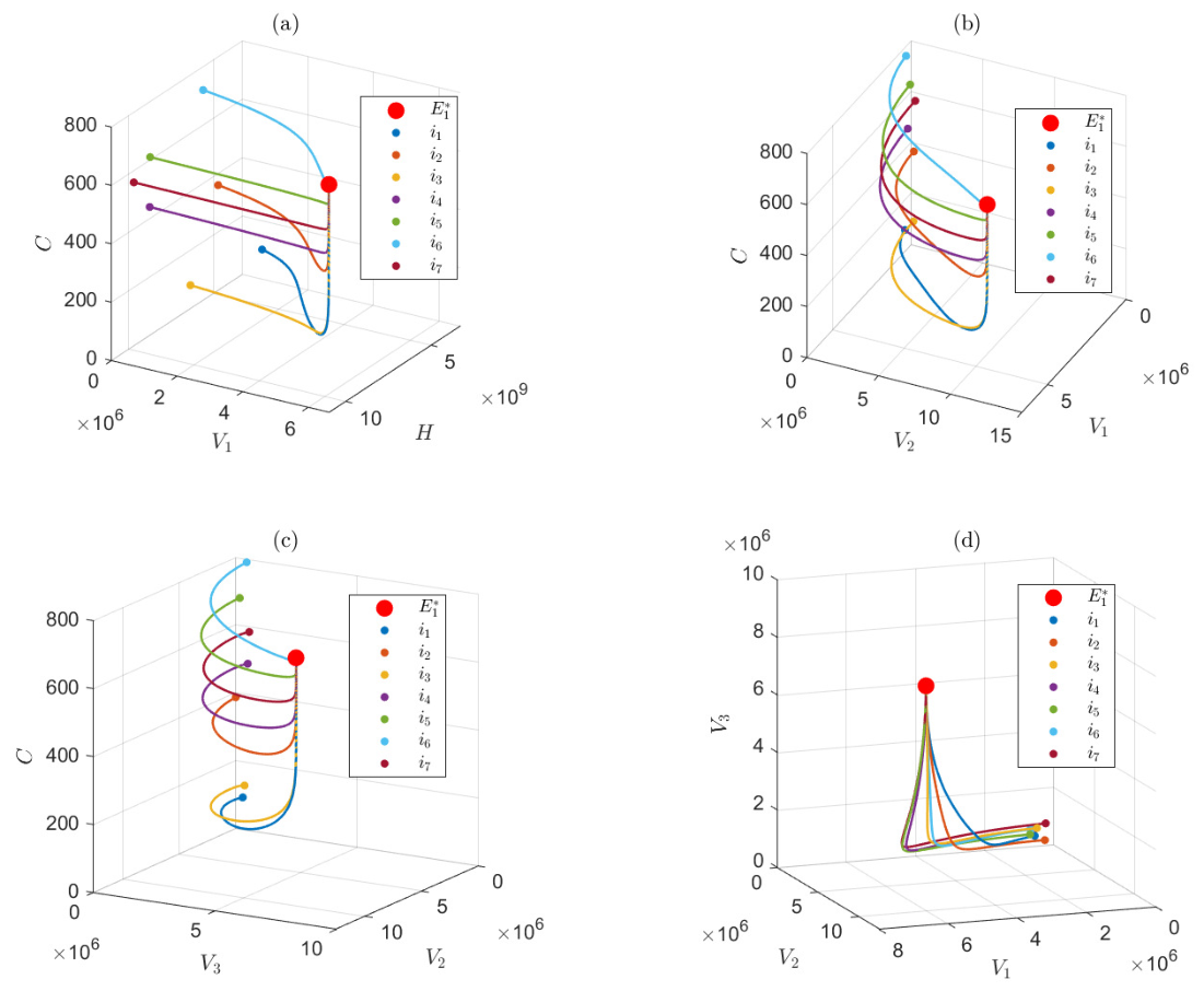
In this section, we present numerical simulations to validate the global asymptotic stability of the interior equilibrium E 1 * = ( H * , V 1 * , V 2 * , V 3 * , C * ) , as analytically established in Theorem 5. The simulations are conducted using the parameter values listed in Table 4. To confirm that the system consistently converges to E 1 * , the governing equations are integrated across multiple distinct initial points.
Figure 2a–d displays the phase space trajectories projected onto the H V 1 C , V 1 V 2 C , V 2 V 3 C , and V 1 V 2 V 3 subspaces, respectively, simulated over the time span t [ 0 , 3000 ] .
As illustrated, regardless of their initial points, all trajectories converge to the interior equilibrium point E 1 * . These numerical trajectories verify that the interior equilibrium state is globally attractive and highly robust against variations in initial perturbations. Ultimately, these simulation results strongly align with and validate the formal analytical proof provided in Theorem 5.

5.4. Global Sensitivity Analysis

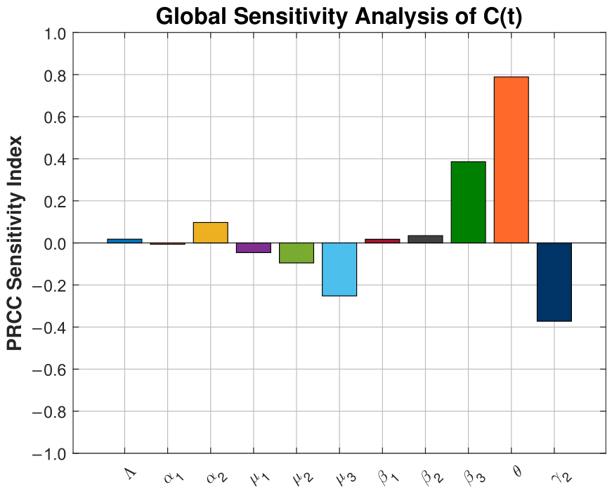
To quantify how individual model parameters influence atmospheric CO2 concentrations, we employed Latin Hypercube Sampling (LHS) in conjunction with Partial Rank Correlation Coefficient (PRCC) analysis. This LHS–PRCC framework provides a robust global sensitivity measure, where the absolute magnitude of the PRCC (ranging from 0 to 1) identifies the parameters with the most significant impact on model outcomes [38,39]. Within this context, the sign of the coefficient dictates the direction of influence: positive PRCC values indicate a direct relationship, whereas negative values signify an inverse relationship [40].
For the LHS matrix generation, all parameters in model (1) were assigned uniform distributions. To ensure statistical convergence and the robustness of the resulting PRCCs, a sample size of N = 3000 was generated. This global analysis was executed by perturbing each parameter within a ± 50 % range of its established baseline value, thereby providing a comprehensive view of the system’s sensitivity and capturing potential extreme real-world scenarios.
The ranking of parameters based on their absolute PRCC values is presented in Table 5. The results indicate that the human activity emission coupling factor ( θ ) is the most influential parameter, with the highest PRCC value ( + 0.789 ). This strong influence suggests that human-driven activities such as energy consumption, industrial processes, and land-use changes play a dominant role in determining atmospheric CO2 levels. Therefore, reductions in emissions associated with these activities could significantly decrease atmospheric CO2 concentration.
The CO2 emission rate from old-aged vehicles ( β 3 ) is identified as the second-most-influential parameter (PRCC = + 0.386 ). This finding highlights the substantial contribution of older vehicles to atmospheric CO2 emissions, mainly due to inefficient combustion systems and outdated emission-control technologies. Closely following this is the anthropogenic depletion coefficient ( γ 2 ), which ranks third with a strong negative sensitivity of 0.372 . This inverse relationship highlights the critical role of mitigation strategies, such as reforestation and carbon sequestration, in actively counterbalancing atmospheric accumulation.
Finally, parameters governing vehicle lifecycles, specifically the retirement rate of old-aged vehicles ( μ 3 ) demonstrate a moderate yet noticeable influence (PRCC = 0.252 ). This suggests that while sequestration and industrial regulations are primary levers, accelerating the removal of inefficient vehicles from the transport network provides a significant secondary benefit for climate stabilization.
The sensitivity analysis presented in Figure 3 identifies θ and β 3 as the parameters with the most significant positive PRCC values. This confirms that atmospheric CO2 accumulation is most strongly driven by human activity emissions and the output from aging vehicle fleets.
Conversely, the parameter γ 2 shows a strong negative sensitivity, indicating that it plays an important role in reducing atmospheric CO2 concentration. The simulation results show that increasing γ 2 leads to a decrease in CO2 levels. Similarly, the parameter μ 3 , which represents the retirement rate of old vehicles, also has a negative effect on CO2 levels.
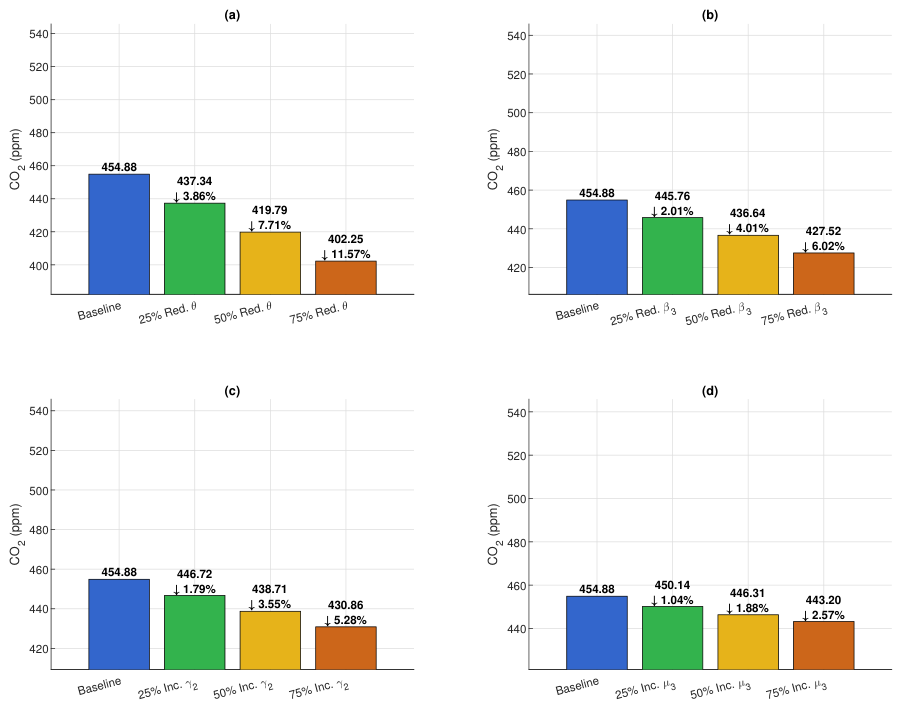
Figure 4 presents a comparative sensitivity analysis of projected CO2 concentrations over 30-years. As illustrated in Figure 4a, reducing the human activity emission factor ( θ ) yields the most substantial decline in atmospheric CO2 concentration, notably, a 25% reduction in θ lowers the projected CO2 level from 454.88 ppm to 436.7 ppm. Similarly, Figure 4b reveals that decreasing the emission rate of old vehicles ( β 3 ) markedly reduces overall CO2 concentrations. In contrast, Figure 4c demonstrates that increasing the anthropogenic CO2 removal coefficient ( γ 2 ) enhances carbon sequestration capacity. Finally, Figure 4d indicates that accelerating the retirement rate of old vehicles ( μ 3 ) further contributes to CO2 mitigation by removing high-emitting vehicles from system.

6. Results and Discussion

Balancing atmospheric CO2 mitigation with the continuously increasing demand for transportation remains one of the defining challenges of sustainable development. In this study, we developed and analyzed a nonlinear mathematical model of atmospheric CO2 dynamics by coupling atmospheric carbon concentration with human population growth and an age-structured vehicle population. Unlike many existing mathematical models that treat transportation emissions as a homogeneous source, the proposed model explicitly accounts for the differential contributions of vehicle cohorts by age. This enables the model to capture the elevated emissions associated with aging vehicle fleets and their long-term influence on atmospheric carbon accumulation.
The qualitative analysis demonstrated that the solutions of the model remain positive and bounded for all biologically feasible initial conditions, confirming the physical relevance of the proposed framework. The stability analysis further showed that the boundary equilibrium point, E 0 * , is unstable, whereas the interior equilibrium point, E 1 * , is globally asymptotically stable. From an environmental perspective, these findings proved that the coupled human–vehicle–atmospheric system naturally evolves toward a persistent equilibrium characterized by non-zero atmospheric CO2 concentrations.
This interpretation is consistent with the findings of large-scale climate assessments. According to the Intergovernmental Panel on Climate Change (IPCC) report [41], continued economic and population growth, together with ongoing dependence on fossil fuels, will continue to increase greenhouse gas emissions unless effective mitigation measures are implemented. Similarly, analyses of the global carbon budget show that current emission trends are not consistent with the pathways needed to limit global warming to internationally agreed targets [42]. Therefore, the mathematical stability results obtained in this study provide theoretical support for the empirical evidence that atmospheric carbon accumulation is unlikely to decline on its own without deliberate policy interventions.
Using historical data, model calibration, and parameter estimation, projected an atmospheric CO2 concentration of approximately 455 ppm by the year 2040 if present trends persist. This estimate falls within the range suggested by previous climate investigations and stabilization studies. For example, den Elzen et al. [43] showed that delayed mitigation efforts substantially increase the likelihood of exceeding stabilization thresholds, while Mukherji et al. [44] highlighted that continued anthropogenic forcing under current development trajectories results in sustained increases in atmospheric carbon concentrations. Moreover, observational records reported by NASA [45] continue to document a persistent rise in atmospheric CO2, reinforcing the plausibility of our model projections. The agreement between our model and these climate assessments suggests that such Mathematical models can effectively reproduce the dominant mechanisms governing long-term atmospheric carbon dynamics.
The global sensitivity analysis based on the Partial Rank Correlation Coefficient (PRCC) method identified human-related activities as the most influential determinants of atmospheric CO2 accumulation. This result agrees with the broad scientific consensus that energy consumption, industrial activities, land-use change, and population-driven demand are the principal drivers of anthropogenic climate change [41,42].
More importantly, our analysis identified the emission rate associated with older vehicles as the second-most-influential parameter affecting future atmospheric carbon levels. This finding extends previous transportation studies by demonstrating that fleet composition may be as important as fleet size in determining long-term environmental outcomes. Transportation research has consistently shown that older vehicles emit substantially higher levels of pollutants because of technological obsolescence, engine deterioration, and the absence of modern emission-control systems. Studies by Anenberg et al. [46] and Barrett et al. [47], for example, reported that replacing aging vehicle fleets with cleaner technologies yields considerable environmental and public-health benefits. Similarly, assessments by the International Energy Agency have emphasized that improvements in vehicle efficiency can be offset by slow fleet turnover and increasing travel demand [48]. By explicitly incorporating vehicle age structure, the present model provides a mathematical explanation for these empirical observations and identifies aging vehicles as a critical leverage point for intervention.

7. Recommendations

The PRCC analysis identified the human activity emission coupling factor, θ , as the most influential parameter governing atmospheric CO2 accumulation. Consequently, emission-reduction policies should primarily target sectors associated with human activities, including energy production, industrial processes, and land-use practices. The sensitivity analysis further indicates that a 25% reduction in the human activity emission parameter could decrease the projected atmospheric CO2 concentration by approximately 17 ppm by 2040 relative to the baseline projection. This finding suggests that interventions aimed at improving energy efficiency, expanding renewable energy deployment, and promoting low-carbon production practices would have the greatest impact on mitigating future atmospheric CO2 accumulation.
The older-vehicle emission parameter, β 3 , was identified as the second-most-influential factor affecting atmospheric CO2 dynamics. This result demonstrates that aging vehicle fleets contribute disproportionately to long-term carbon accumulation. The model predicts that a 25% reduction in emissions from older vehicles could lower the projected atmospheric CO2 concentration by approximately 9 ppm by 2040. Therefore, transportation policies should prioritize accelerated fleet renewal through stricter vehicle inspection and maintenance programs, vehicle scrappage incentives, the enforcement of emission standards for aging vehicles, and increased support for the adoption of cleaner and electric vehicle technologies.
Furthermore, the anthropogenic CO2 depletion parameter, γ 2 , was found to play an important role in mitigating atmospheric carbon accumulation. Sensitivity analysis indicates that increasing the effective anthropogenic CO2 removal rate by 25% could reduce the projected atmospheric CO2 concentration by approximately 8 ppm by 2040. Accordingly, governments and stakeholders should establish measurable targets for expanding reforestation and afforestation programs and invest in carbon capture, utilization, and storage technologies to enhance atmospheric carbon removal.

8. Future Work

In future research, the model can be extended to include additional factors, such as electric vehicles and the adoption of renewable energy.

Author Contributions

A.K.M.: conceptualization of the study; development of the methodology; formulation of the mathematical model; and preparation of the original draft manuscript. E.M.A.: conceptualization of the study; development and implementation of the MATLAB code; numerical simulations; and critical review and editing of the manuscript. G.T.A.: conceptualization of the study; development of MATLAB code; model validation; numerical verification of results; and review and editing of the manuscript. P.J.W.: conceptualization of the study; supervision of the research project; guidance on theoretical analysis; project administration; and critical review and editing of the manuscript. Y.A.B.: conceptualization of the study; analytical analysis of the model; investigation and interpretation of results; and review and editing of the manuscript. All authors have read and agreed to the published version of the manuscript.

Funding

This research received no external funding.

Data Availability Statement

No data was generated for or during this research. All the data used are publicly available and are referenced in this manuscript.

Conflicts of Interest

The authors declare no conflict of interest.

References

  1. Riaz, M.B.; Raza, N.; Martinovic, J.; Bakar, A.; Tunç, O. Modeling and simulations for the mitigation of atmospheric carbon dioxide through forest management programs. AIMS Math. 2024, 9, 22712–22742. [Google Scholar] [CrossRef] [Scilit]
  2. Nunes, L.J. The rising threat of atmospheric CO2: A review on the causes, impacts, and mitigation strategies. Environments 2023, 10, 66. [Google Scholar] [CrossRef] [Scilit]
  3. Hansen, J.; Sato, M. Greenhouse gas growth rates. Proc. Natl. Acad. Sci. USA 2004, 101, 16109–16114. [Google Scholar] [CrossRef] [Scilit] [PubMed]
  4. Raihan, A.; Begum, R.A.; Nizam, M.; Said, M.; Pereira, J.J. Dynamic impacts of energy use, agricultural land expansion, and deforestation on CO2 emissions in Malaysia. Environ. Ecol. Stat. 2022, 29, 477–507. [Google Scholar] [CrossRef] [Scilit]
  5. Donald, P.; Mayengo, M.; Lambura, A.G. Mathematical modeling of vehicle carbon dioxide emissions. Heliyon 2024, 10, e23976. [Google Scholar] [CrossRef] [Scilit] [PubMed]
  6. Kabir, M.; Habiba, U.; Iqbal, M.; Shafiq, M.; Farooqi, Z.; Shah, A.; Khan, W. Impacts of anthropogenic activities & climate change resulting from increasing concentration of carbon dioxide on environment in 21st century: A critical review. IOP Conf. Ser. Earth Environ. Sci. 2023, 1194. [Google Scholar] [CrossRef] [Scilit]
  7. Pedreira, V.N.; Brito, M.L.; Santos, L.C.L.d.; Simonelli, G. Modeling of Brazilian carbon dioxide emissions: A review. Braz. Arch. Biol. Technol. 2022, 65, e22210594. [Google Scholar] [CrossRef] [Scilit]
  8. Zhao, X.; Mahendra, A.; Godfrey, N.; Dalkmann, H.; Rode, P.; Floater, G. Unlocking the Power of Urban Transit Systems for Better Growth and a Better Climate; Technical Note; New Climate Economy: London, UK; Washington, DC, USA, 2015. [Google Scholar]
  9. Gu, J.; Jiang, S.; Zhang, J.; Jiang, J. An analysis of the decomposition and driving force of carbon emissions in transport sector in China. Sci. Rep. 2024, 14, 30177. [Google Scholar] [CrossRef] [Scilit] [PubMed]
  10. Ferrer, A.L.C.; Thome, A.M.T. Carbon emissions in transportation: A synthesis framework. Sustainability 2023, 15, 8475. [Google Scholar] [CrossRef] [Scilit]
  11. Pryciński, P.; Pielecha, J.; Korzeb, J.; Jachimowski, R.; Pielecha, P. Impact of vehicle aging and mileage on air pollution emissions. Energies 2025, 18, 939. [Google Scholar] [CrossRef] [Scilit]
  12. Singam, V.T.; Rafiuddin, N.M.; Zahari, H.M. Factors of Old Vehicles Contributing to Air Pollution in The Urban Environment. Int. J. Acad. Res. Bus. Soc. Sci. 2024, 14, 962–972. [Google Scholar] [CrossRef] [Scilit]
  13. Ene Yalçın, S. Estimation of CO2 emissions in transportation systems using artificial neural networks, machine learning, and deep learning: A comprehensive approach. Systems 2025, 13, 194. [Google Scholar] [CrossRef] [Scilit]
  14. Misra, A.K.; Jha, A. Modeling the effect of budget allocation on the abatement of atmospheric carbon dioxide. Comput. Appl. Math. 2022, 41, 202. [Google Scholar] [CrossRef] [Scilit]
  15. Sundar, S.; Mishra, A.K.; Naresh, R.; Shukla, J. Modeling the impact of population density on carbon dioxide emission and its control: Effects of greenbelt plantation and seaweed cultivation. Model. Earth Syst. Environ. 2019, 5, 833–841. [Google Scholar] [CrossRef] [Scilit]
  16. Fors, W. Population and Greenhouse Gas Dynamics: An Implementation of System Dynamics. Master’s Thesis, University of Vaasa, Vaasa, Finland, 2021. [Google Scholar]
  17. Misra, A.; Verma, M.; Venturino, E. Modeling the control of atmospheric carbon dioxide through reforestation: Effect of time delay. Model. Earth Syst. Environ. 2015, 1, 24. [Google Scholar] [CrossRef] [Scilit]
  18. Caetano, M.A.L.; Gherardi, D.F.M.; Yoneyama, T. Optimal resource management control for CO2 emission and reduction of the greenhouse effect. Ecol. Model. 2008, 213, 119–126. [Google Scholar] [CrossRef] [Scilit]
  19. Devi, S.; Gupta, N. Dynamics of carbon dioxide gas (CO2): Effects of varying capability of plants to absorb CO2. Nat. Resour. Model. 2019, 32, e12174. [Google Scholar]
  20. Mehmood, A.; Hassan, M.; Ali, I.; Jawo, E. A mathematical model for optimizing global warming caused by carbon dioxide emissions from energy sector. AIP Adv. 2025, 15, 025223. [Google Scholar] [CrossRef] [Scilit]
  21. Liu, S.; Chen, S.; Liang, X.; Mao, B.; Jia, S. Analysis of transport policy effect on CO2 emissions based on system dynamics. Adv. Mech. Eng. 2015, 7, 323819. [Google Scholar]
  22. Chang, X.; Chen, B.Y.; Li, Q.; Cui, X.; Tang, L.; Liu, C. Estimating real-time traffic carbon dioxide emissions based on intelligent transportation system technologies. IEEE Trans. Intell. Transp. Syst. 2012, 14, 469–479. [Google Scholar] [CrossRef] [Scilit]
  23. Ospina, D.; Zapata, S.; Castañeda, M.; Dyner, I.; Aristizábal, A.J.; Escalante, N. Model for evaluating CO2 emissions and the projection of the transport sector. Int. J. Electr. Comput. Eng. 2018, 8, 1781. [Google Scholar] [CrossRef] [Scilit]
  24. Misra, A.; Jha, A. How to combat atmospheric carbon dioxide along with development activities? A mathematical model. Phys. D. Nonlinear Phenom. 2023, 454, 133861. [Google Scholar] [CrossRef] [Scilit]
  25. Verma, M.; Verma, A.K. Effect of plantation of genetically modified trees on the control of atmospheric carbon dioxide: A modeling study. Nat. Resour. Model. 2021, 34, e12300. [Google Scholar] [CrossRef] [Scilit]
  26. Brauer, F.; Castillo-Chavez, C.; Feng, Z. Mathematical Models in Epidemiology; Springer: New York, NY, USA, 2019; Volume 32. [Google Scholar]
  27. Cinch. When Does a New Car Need a Service? Available online: https://www.cinch.co.uk/guides/car-maintenance/new-car-first-service (accessed on 21 February 2026).
  28. Fleetio. Fleet Vehicle Replacement Timeline: How to Know It’s Time? Available online: https://www.fleetio.com/blog/how-to-calculate-vehicle-replacement-timeline (accessed on 21 February 2026).
  29. Cartrack. Used Car Mileage vs. Age: What’s More Important When Buying a Car? Available online: https://www.cartrack.co.za/blog/used-car-mileage-vs-age-whats-more-important-when-buying-a-car (accessed on 21 February 2026).
  30. NOAA. Climate Change: Atmospheric Carbon Dioxide. Available online: https://gml.noaa.gov/webdata/ccgg/trends/co2/co2_annmean_mlo.txt (accessed on 29 March 2026).
  31. UN. World Population Prospects. Available online: https://www.un.org/development/desa/pd/sites/www.un.org.development.desa.pd/files/files/documents/2020/Jan/un_2010_world_population_prospects-2010_revision_volume-i_comprehensive-tables.pdf (accessed on 29 March 2026).
  32. Statista. Number of Passenger Cars and Commercial Vehicles in Use Worldwide from 2006 to 2015. Available online: https://www.statista.com/statistics/281134/number-of-vehicles-in-use-worldwide/?srsltid=AfmBOoptL7G2TC7fVhJkCSO8KMq9HFEY60eln8bzB_X2j8K_w-wXeU9c (accessed on 21 February 2026).
  33. Moriasi, D.N.; Arnold, J.G.; Van Liew, M.W.; Bingner, R.L.; Harmel, R.D.; Veith, T.L. Model evaluation guidelines for systematic quantification of accuracy in watershed simulations. Trans. ASABE 2007, 50, 885–900. [Google Scholar] [CrossRef] [Scilit]
  34. Boulange, J.; Nizamov, S.; Nurbekov, A.; Ziyatov, M.; Kamilov, B.; Nizamov, S.; Abduvasikov, A.; Khamdamova, G.; Watanabe, H. Calibration and validation of the AquaCrop model for simulating cotton growth under a semi-arid climate in Uzbekistan. Agric. Water Manag. 2025, 310, 109360. [Google Scholar] [CrossRef] [Scilit]
  35. Fandel, G.; Letmathe, P.; Spengler, T.S.; Walther, G. Sustainable operations. J. Bus. Econ. 2021, 91, 123–125. [Google Scholar]
  36. Ritter, A.; Muñoz-Carpena, R. Performance evaluation of hydrological models: Statistical significance for reducing subjectivity in goodness-of-fit assessments. J. Hydrol. 2013, 480, 33–45. [Google Scholar] [CrossRef] [Scilit]
  37. Moriasi, D.N.; Gitau, M.W.; Pai, N.; Daggupati, P. Hydrologic and water quality models: Performance measures and evaluation criteria. Trans. ASABE 2015, 58, 1763–1785. [Google Scholar] [CrossRef] [Scilit]
  38. Marino, S.; Hogue, I.B.; Ray, C.J.; Kirschner, D.E. A methodology for performing global uncertainty and sensitivity analysis in systems biology. J. Theor. Biol. 2008, 254, 178–196. [Google Scholar] [CrossRef] [Scilit] [PubMed]
  39. Khondaker, F.; Kamrujjaman, M.; Islam, M.S. Cost-effectiveness of dengue control strategies in Bangladesh: An optimal control and ACER-ICER analysis. Acta Trop. 2025, 264, 107587. [Google Scholar] [CrossRef] [Scilit] [PubMed]
  40. Fanuel, I.M.; Mirau, S.; Kajunguri, D.; Moyo, F. Conservation of forest biomass and forest–dependent wildlife population: Uncertainty quantification of the model parameters. Heliyon 2023, 9, e16948. [Google Scholar] [CrossRef] [Scilit] [PubMed]
  41. Shukla, P.; Skea, J.; Slade, R.; Al Khourdajie, A.; van Diemen, R.; McCollum, D.; Pathak, M.; Some, S.; Vyas, P.; Fradera, R.; et al. IPCC Summary for Policymakers Sixth Assessment Report (WG3). Clim. Change 2022, 3–48. [Google Scholar] [CrossRef] [Scilit]
  42. IEA. Global EnergyReview 2025. Available online: https://www.iea.org/reports/global-energy-review-2025 (accessed on 21 March 2026).
  43. Den Elzen, M.G.; Van Vuuren, D.P. Peaking profiles for achieving long-term temperature targets with more likelihood at lower costs. Proc. Natl. Acad. Sci. USA 2007, 104, 17931–17936. [Google Scholar] [CrossRef] [Scilit] [PubMed]
  44. Mukherji, A. Climate Change 2023 Synthesis Report. Available online: https://www.ipcc.ch/report/ar6/syr/ (accessed on 29 March 2026).
  45. NASA. Graphic: Carbon Dioxide Hits New High. Available online: https://science.nasa.gov/resource/graphic-carbon-dioxide-hits-new-high/ (accessed on 29 March 2026).
  46. Anenberg, S.C.; Miller, J.; Minjares, R.; Du, L.; Henze, D.K.; Lacey, F.; Malley, C.S.; Emberson, L.; Franco, V.; Klimont, Z.; et al. Impacts and mitigation of excess diesel-related NOx emissions in 11 major vehicle markets. Nature 2017, 545, 467–471. [Google Scholar] [CrossRef] [Scilit] [PubMed]
  47. Barrett, S.R.H.; Speth, R.L.; Eastham, S.D.; Dedoussi, I.C.; Ashok, A.; Malina, R.; Keith, D.W. Impact of the Volkswagen emissions control defeat device on US public health. Environ. Res. Lett. 2015, 10, 114005. [Google Scholar] [CrossRef] [Scilit]
  48. International Energy Agency. Global EV Outlook 2024: Moving Towards Increased Affordability; International Energy Agency: Paris, France, 2024. [Google Scholar]
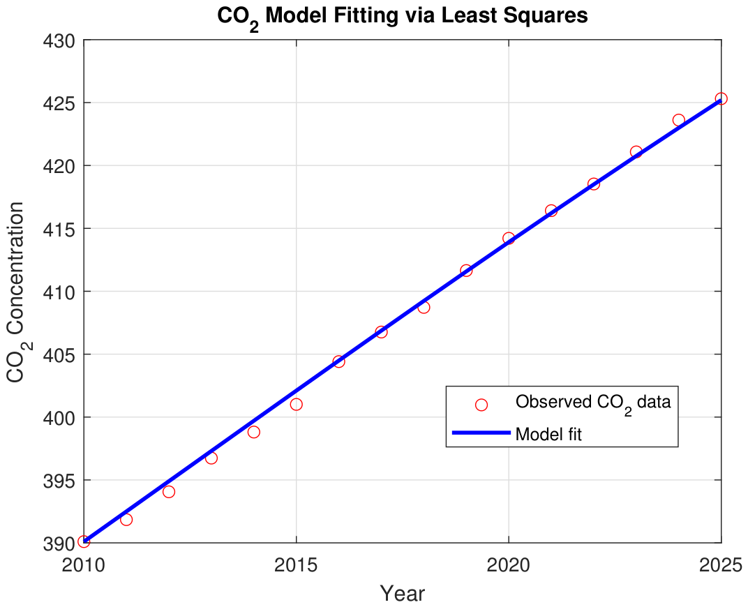
Figure 1. Observed versus fitted atmospheric CO2 concentrations from 2010 to 2025. Red circles indicate the observed CO2 data, while the blue line represents the model fit.
Appliedmath 06 00122 g001
Figure 2. Phase space trajectories verifying the global asymptotic stability of the interior equilibrium E 1 * . Specifically, subplot (a) shows the H V 1 C subspace, demonstrating the simultaneous convergence of the human population ( H ), the new vehicle cohort ( V 1 ), and the atmospheric CO 2 concentration ( C ) towards ( H * , V 1 * , C * ) = ( 1.1 × 10 10 , 6.6473 × 10 6 , 781.66 ) . Subplot (b) presents the V 1 V 2 C subspace, highlighting the convergence of the new ( V 1 ) and mid-aged ( V 2 ) vehicle cohorts alongside carbon dynamics toward ( V 1 * , V 2 * , C * ) = ( 6.6473 × 10 6 , 1.26 × 10 7 , 781.66 ) . Similarly, subplot (c) maps the V 2 V 3 C subspace, tracking the trajectories of the mid-aged ( V 2 ) and old vehicle ( V 3 ) cohorts relative to atmospheric carbon accumulation as they approach ( V 2 * , V 3 * , C * ) = ( 1.26 × 10 7 , 8.343 × 10 6 , 781.66 ) . Finally, subplot (d) isolates the V 1 V 2 V 3 subspace, illustrating the joint evolution of the entire vehicular fleet toward ( V 1 * , V 2 * , V 3 * ) = ( 6.6473 × 10 6 , 1.26 × 10 7 , 8.343 × 10 6 ) .
Appliedmath 06 00122 g002
Figure 3. Global sensitivity analysis of atmospheric CO2 concentration using PRCC. The bar chart shows the influence of model parameters, where positive values indicate increasing effects on CO2 and negative values indicate decreasing effects.
Appliedmath 06 00122 g003
Figure 4. Sensitivity analysis of the predicted 2040 CO2 concentration to parameter perturbations. Reducing the human activity emission factor ( θ ) leads to the largest decline in atmospheric CO2 concentration, indicating that human-related emissions are the dominant driver of CO2 accumulation in the system. Similarly, reducing the emission rate from old vehicles ( β 3 ) significantly decreases CO2 levels. In contrast, increasing the anthropogenic CO2 removal coefficient ( γ 2 ) enhances carbon sequestration capacity. Finally, increasing the retirement rate of old vehicles ( μ 3 ) also contributes to CO2 reduction by removing high-emission vehicles from circulation, though its impact is relatively smaller compared to θ and β 3 .
Appliedmath 06 00122 g004
Table 1. Model state variables and their description.
State VariablesDescription
H ( t ) Human population size at time t
V 1 ( t ) New vehicle cohort (mileage < 30 , 000 miles)
V 2 ( t ) Mid-aged vehicle cohort (mileage 30 , 000 100 , 000 miles)
V 3 ( t ) Old vehicle cohort (mileage > 100 , 000 miles)
C ( t ) Cumulative atmospheric CO 2 concentration
Table 2. Model parameters and their description.
ParametersDescription
s Intrinsic growth rate of the human population
K Environmental carrying capacity for the human population
Λ Per capita vehicle acquisition rate
α 1 , α 2 Transition rates between vehicle age cohorts (aging rates)
μ i Retirement/scrapping rates for vehicle class i ( i = 1 , 2 , 3 )
β i CO 2 emission intensity of vehicle class i ( i = 1 , 2 , 3 )
θ Human activity emission coupling factor (energy consumption, industrial processes, land-use changes)
δ Constant emission rate from natural and biological respiration processes
γ 1 Natural CO 2 depletion coefficient (oceanic and terrestrial sinks)
γ 2 Anthropogenic CO 2 removal coefficient (sequestration and reforestation)
Table 3. Atmospheric CO2 concentration (ppm) from 2010 to 2025.
Year20102011201220132014201520162017
CO2 (ppm)390.1391.85394.06396.74398.81401.01404.41406.76
Year20182019202020212022202320242025
CO2 (ppm)408.72411.65414.21416.41418.53421.08423.61425.31
Table 4. Parameter values and their corresponding units.
ParametersValueUnitSource
H ( 0 ) 6.96 × 10 9 Person[31]
V 1 ( 0 ) 2.5375 × 10 8 Vehicle[27,28,29,32]
V 2 ( 0 ) 4.5675 × 10 8 Vehicle[27,28,29,32]
V 3 ( 0 ) 3.405 × 10 8 Vehicle[27,28,29,32]
C ( 0 ) 390.1 ppm[30]
s 0.046 1 / Year Fitted
K 11 × 10 9 Person[25]
Λ 1.04 × 10 4 Vehicle/(Person · Year)Fitted
α 1 0.164 1 / Year Fitted
α 2 3.789 × 10 2 1 / Year Fitted
μ 1 8.109 × 10 3 1 / Year Fitted
μ 2 4.87 × 10 2 1 / Year Fitted
μ 3 5.715 × 10 2 1 / Year Fitted
β 1 2.187 × 10 10 ppm/(Vehicle · Year)Fitted
β 2 6.836 × 10 10 ppm/(Vehicle · Year)Fitted
β 3 4.912 × 10 9 ppm/(Vehicle · Year)Fitted
θ 3.02 × 10 10 ppm/(Person · Year)Fitted
δ 0.035 ppm/YearFitted
γ 1 0.0016 ppm/YearFitted
γ 2 0.00276 ppm/YearFitted
Table 5. Parameter ranking (most influential first).
RankParameterPRCC Value
1 θ + 0.789
2 β 3 + 0.386
3 γ 2 0.372
4 μ 3 0.252
5 α 2 + 0.0973
6 μ 2 0.0951
7 μ 1 0.0461
8 β 2 + 0.0346
9 Λ + 0.018
10 β 1 + 0.0173
11 α 1 0.00643
Disclaimer/Publisher’s Note: The statements, opinions and data contained in all publications are solely those of the individual author(s) and contributor(s) and not of MDPI and/or the editor(s). MDPI and/or the editor(s) disclaim responsibility for any injury to people or property resulting from any ideas, methods, instructions or products referred to in the content.