1. Introduction
Previous studies on jagged boundaries in continuum topology optimization have mainly focused on boundary reconstruction, post-processing, and direct smooth-boundary representation [
1,
2]. Fu [
3] fitted optimized boundaries using geometric reconstruction techniques, and Zhang [
4] removed gray elements through binarization and extracted boundary corner points for curve fitting. Li et al. [
5] used a pre-built lookup table to transform local boundary-element shapes, thereby improving jagged boundaries in topology optimization results. Although these post-processing-based methods can improve the geometric quality of the final topology, the smoothing operation is usually performed after optimization and is not directly involved in the topology-evolution process. Consequently, the mechanical response of the post-processed geometry may differ from that of the original finite element model.
For direct smooth-boundary representation, Da et al. [
6] constructed a level-set function using nodal sensitivity to obtain smooth boundaries for continuum structures. Liu et al. [
7] investigated stress optimization of smooth continuum structures, and Fu et al. [
8] achieved smooth three-dimensional topology design based on elemental volume fractions and a zero level-set function. Yu introduced a smoothing technique into the Moving Morphable Components (MMC) framework and improved boundary continuity through convolution control [
9]. Level-set methods describe structural boundaries implicitly through level-set functions, whereas MMC-based methods represent structural layouts explicitly through movable morphable components. In contrast to these methods, the present study is developed within the ICM-MMSB framework and focuses on boundary extraction, remeshing, and topology-variable transfer during optimization.
In addition to post-processing and smooth-boundary reconstruction, adaptive meshing provides an important means of improving boundary quality. Maute and Ramm [
10] were among the first to propose adaptive topology optimization methods, which improve the representational accuracy of critical regions through local mesh adjustment. Thomás et al. [
11] proposed an adaptive refinement strategy based on polygonal meshes, obtaining clearer material distributions and boundaries while reducing computational cost. Wang et al. [
12] further developed an adaptive mesh-refinement strategy for manufacturability, showing that mesh refinement can improve both boundary quality and manufacturable structural layouts. Related developments include h/r-type adaptive meshes with level-set pruning meshes for stress-constrained shape and topology optimization [
13], adaptive refinement combined with mesh deformation [
14], conformal adaptive meshes combined with Helmholtz-type filtering [
15], full-scale three-dimensional topology optimization based on level sets and adaptive meshing [
16], adaptive mesh refinement and level-set methods for compliant mechanisms [
17], and an adaptive mesh-based SBFE-BESO method for multi-material topology optimization [
18]. Overall, these studies have improved the representation accuracy of boundary regions and the quality of optimized configurations. However, for optimization procedures involving repeated remeshing, topology-information transfer between different meshes remains a key issue. After remeshing, the element numbers, node locations, and element connectivity of the current analysis mesh change; therefore, topology variables defined on the old mesh cannot be directly used on the new mesh. If the topology-variable field is not properly inherited, the local material distribution may be lost or distorted, and the continuity of topology evolution may be affected. This issue is particularly important for boundary-moving methods because subsequent boundary extraction and remeshing depend on the inherited topology-variable field.
Compared with the above methods, the Independent Continuous Mapping (ICM) method focuses on unifying the relationship between discrete topology variables and continuous optimization solutions at the modeling level. Sui [
19] first proposed the ICM method by restoring the independence of topological design variables through the separation of topology variables from material or geometric parameters. Peng [
20] subsequently improved the ICM method, and Ye [
21] further promoted its engineering implementation in static topology optimization of continuum structures and related software development. For specific applications, Sui [
22] applied the ICM method to continuum topology optimization under static displacement and frequency constraints, extended it to forced harmonic vibration problems [
23], and proposed a first-order approximation method for internal forces in stress-constrained topology optimization [
24]. Long extended ICM modeling through filter-function combinations [
25], node-independent variable interpolation [
26], and harmonic-response continuum topology optimization [
27]. Yan et al. [
28] investigated the influence of power-law filter parameters on the convergence of topology optimization, and Du et al. [
29,
30] extended the ICM method to continuum topology optimization problems under multi-constraint fail-safe and stochastic damage conditions. To address boundary serration within the ICM framework, Du et al. [
31] proposed the Movable Morphable Smooth-Boundary (MMSB) method. This method uses a triangular mesh and performs boundary identification and remeshing according to threshold contour lines during optimization. It can therefore directly improve jagged boundaries without altering the original mechanical properties of the structure and has achieved satisfactory boundary-smoothing results in numerical examples. Nevertheless, existing MMSB methods mainly focus on smooth-boundary generation, and further improvement is still needed in the stable transfer of topology information before and after remeshing and in the reduction of redundant computations on the updated mesh.
Based on the above review, existing methods have improved boundary quality through post-processing reconstruction, adaptive mesh refinement, level-set-based boundary description, MMC-based geometric representation, and the original MMSB method. However, post-processing methods are usually not involved in topology evolution, and remeshing-based methods must carefully address topology-variable transfer between different meshes. The original MMSB method can move smooth boundaries during optimization, but it mainly focuses on boundary generation; the stable inheritance of topology information before and after remeshing has not been sufficiently considered.
From a broader perspective, the proposed improved MMSB method is related to several existing smooth-boundary topology optimization approaches, but its focus is different. Level Set methods describe structural boundaries implicitly through level-set functions and can naturally provide smooth-boundary representations. MMC-based methods represent structural layouts explicitly using movable morphable components and can describe structural geometry with relatively clear boundaries. Adaptive remeshing techniques improve boundary-region representation by refining, deforming, or regenerating the mesh according to the evolving structural boundary. In contrast, the present method is developed within the ICM-MMSB framework. It does not aim to replace Level Set methods, MMC-based methods, or adaptive remeshing techniques. Instead, it focuses on improving the topology-evolution procedure of the original MMSB method by coupling boundary extraction, remeshing, and topology-variable transfer. In particular, the fixed background mesh is introduced as an intermediate carrier to preserve topology-variable information before and after remeshing. Therefore, the proposed method provides a specific improvement for maintaining topology-information continuity during repeated remeshing while improving boundary representation in the MMSB framework.
Based on this discussion, the main contributions of this study are summarized as follows.
3. Improved MMSB Method
3.1. Original MMSB Method and Its Limitations
The Moving Morphable Smooth-Boundary (MMSB) method was proposed to address the jagged-boundary problem commonly observed in traditional fixed-mesh topology optimization. In ICM-based topology optimization, the mesh serves both as a finite element analysis tool and as a representation of the spatial distribution of topology variables. When the design domain is discretized using a regular quadrilateral mesh, the optimized boundary is usually approximated by element stacking, which can easily produce a stepped contour. This affects the geometric quality of the structural configuration and its subsequent manufacturability. To address this issue, the original MMSB method employs a triangular mesh as the base analysis mesh. During optimization, it extracts isovalue boundaries based on a prescribed threshold and performs remeshing along these boundaries, thereby gradually transforming the structural boundary from a jagged fixed-mesh contour into a smoother geometric boundary. A threshold value of 0.5 is used for boundary identification. When the topology-variable values of adjacent elements cross this threshold, threshold points are obtained through interpolation and then connected to form an isovalue boundary. The mesh is subsequently regenerated based on this boundary. Compared with methods that smooth the boundary only after optimization, the original MMSB method reconstructs the boundary during the optimization iteration process and therefore has advantages in improving boundary quality and manufacturability.
Nevertheless, the original MMSB method still requires further improvement. First, the effectiveness of boundary reconstruction largely depends on the accuracy of threshold-point identification. If the threshold points are not located stably, the extracted isovalue boundaries may contain local discontinuities or geometric deviations, which can affect the subsequent boundary-smoothing results. Second, after each boundary remapping, the number of elements, node numbers, and spatial relationships in the current analysis mesh change, making it difficult to directly map the original topology variables onto the new mesh. Without an effective information-transfer mechanism, the optimization process often requires repeated calculations on the new mesh, which may increase the number of repeated result analyses and hinder the continuity of topology evolution between successive remapping steps. Furthermore, although the original MMSB method achieves boundary smoothing, its overall workflow mainly focuses on boundary generation and does not sufficiently address the complete chain of boundary identification, remeshing, and topology-information inheritance. Therefore, it is necessary to improve threshold-point identification and to establish a stable mechanism for transferring topology variables before and after remeshing, thereby reducing repeated analyses after mesh updating and improving topology-evolution continuity.
3.2. Improved Method and Procedure
To address the limitations of the original MMSB method in boundary-recognition accuracy and topology-information continuity, this study introduces holographic scanning and background mesh mapping to construct an improved MMSB method. The basic idea is as follows. First, the holographic scanning method improves the stability of threshold-point searching and boundary extraction, enabling the isovalue boundary to better reflect the current topology-variable field. Second, by establishing a fixed background mesh, topology-variable information can be mapped and remapped before and after boundary remeshing. This reduces repeated result analyses after mesh updating and improves the continuity of topology evolution.
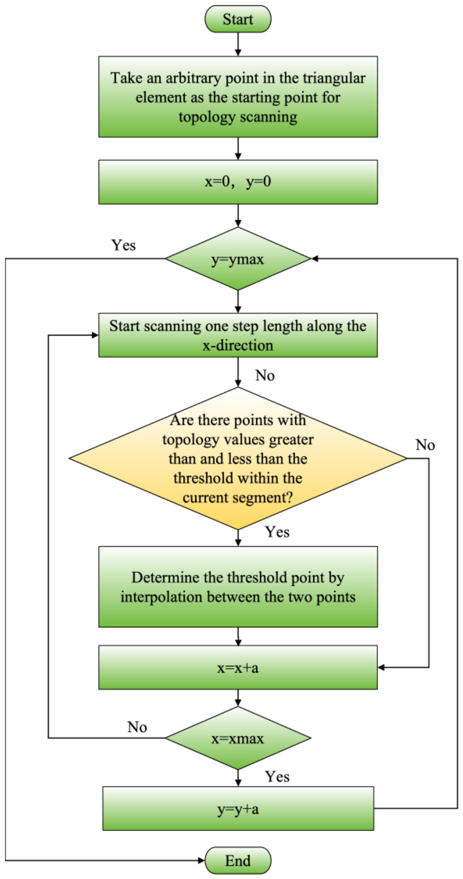
For boundary extraction, the holographic scanning method is used to search the current topology-variable field. First, an arbitrary point in the design domain is selected as the scanning start point. The domain is then scanned segment by segment along the x-direction with a fixed step size. When a scan segment contains topology-variable values both greater than and less than the threshold, linear interpolation is used to determine the coordinate of the boundary point at which the topology-variable value equals the threshold. If no point satisfying this condition is detected within the segment, the scan segment moves forward by one step. After the current row has been scanned, the scan origin returns to the left end and moves one step along the y-direction. This process is repeated until the entire design domain is covered. A series of threshold boundary points is thus obtained in the two-dimensional design domain, and these points are connected to form contour lines representing the structural boundary.
In the holographic scanning process, the design domain is scanned with fixed intervals Δ
x and Δ
y. Let the topology threshold be
η, which is taken as 0.5 in this study. For two adjacent scan points
and
, the corresponding topology-variable values are denoted as
and
respectively. If the following condition is satisfied,
the scan segment between
and
is considered to contain a boundary point. The coordinate of the threshold boundary point
is then calculated by linear interpolation as
After all scan lines are processed, the obtained threshold points are connected according to their spatial order to form the contour boundary used for subsequent remeshing. If the design domain is divided into and scan intervals in the x-directions and y-directions, respectively, the computational complexity of the scanning procedure is .
Where Δ
x and Δ
y are the scanning intervals in the x-directions and y-directions, respectively;
η is the topology threshold used for boundary identification;
and
are two adjacent scan points on the same scan segment;
and
are the topology-variable values corresponding to
and
, respectively; and
denotes the interpolated threshold boundary point.
and
represent the numbers of scan intervals in the x- and y-directions, respectively. The condition
indicates that the topology-variable values on the two sides of the scan segment cross the prescribed threshold, and therefore a boundary point exists between
and
. The flowchart of the holographic scanning method is shown in
Figure 1.
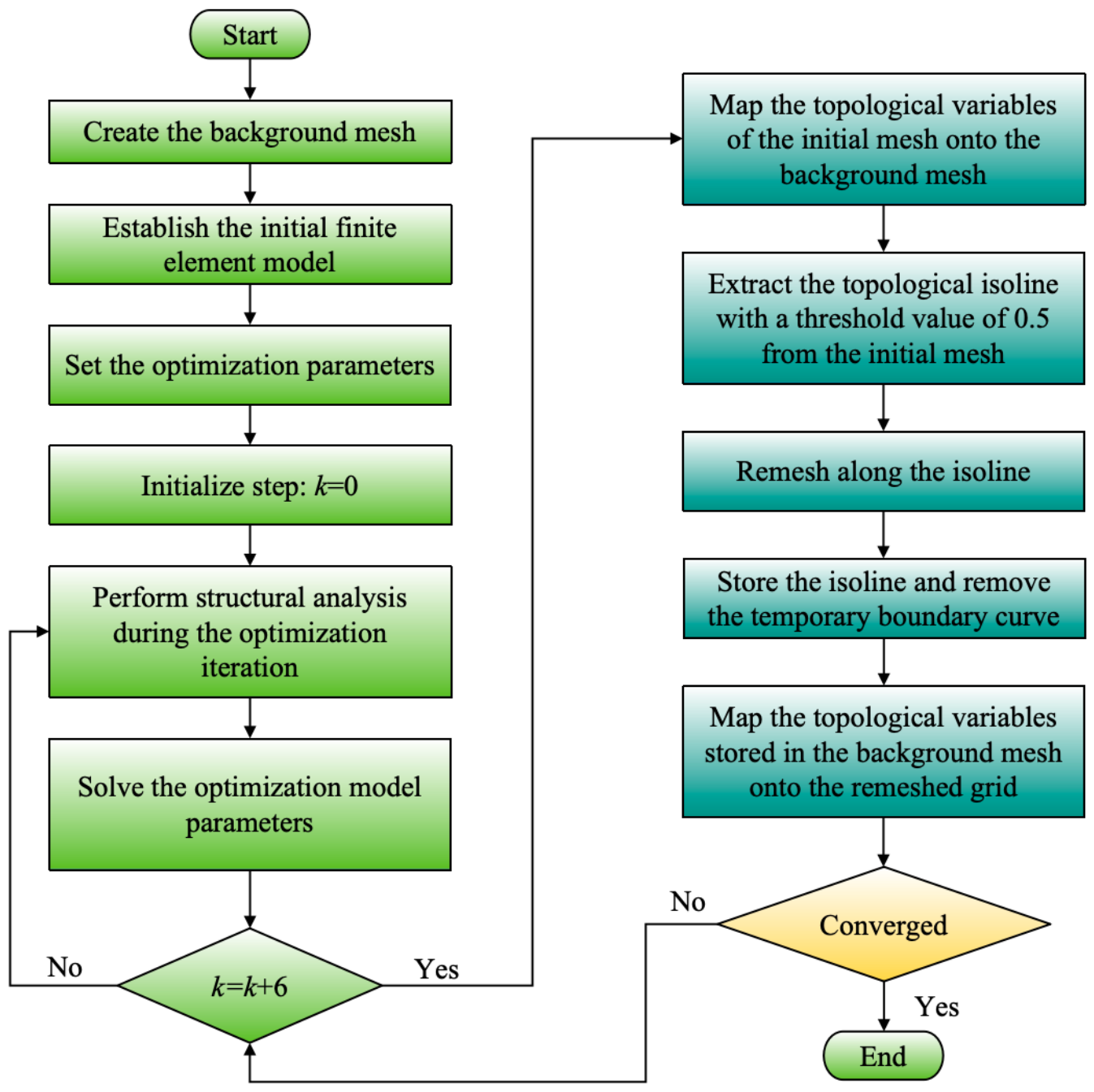
Regarding topology-information transfer, a background mesh mapping technique is introduced to ensure the continuous inheritance of topology variables before and after remeshing. Because the current analysis mesh changes after each boundary remeshing, topology variables on the original mesh cannot be directly mapped to the new mesh. Therefore, this study establishes a fixed background mesh before optimization begins. During optimization, topology information from the current analysis mesh is first mapped to the background mesh for preservation. After boundary extraction is completed and the mesh is regenerated along the contour lines, the topology variables stored on the background mesh are remapped to the new current analysis mesh. Because the node-to-element relationships of the background mesh remain unchanged throughout the optimization process, the background mesh serves as a stable information intermediary between different analysis meshes. With this intermediary, topology variables can be transferred before and after remeshing, thereby reducing repeated result analyses caused by mesh updating and improving the consistency of topology evolution. The overall workflow of the improved MMSB method is shown in
Figure 2.
3.3. Comparison Between the Original MMSB and Improved MMSB Methods
To clarify the methodological differences between the original MMSB method and the improved MMSB method, a direct comparison is presented in this subsection. It should be noted that the proposed method does not aim to establish a completely new topology optimization theory. Instead, its improvement lies in extending the original MMSB framework from a boundary-smoothing procedure to a more complete boundary-evolution procedure that couples boundary extraction, remeshing, and topology-variable transfer.
In the original MMSB method, boundary reconstruction is mainly performed according to the topology-variable distribution on the current analysis mesh. However, when boundary movement and remeshing are carried out, the element numbers, node positions, and element connectivity of the current mesh change. Therefore, topology variables obtained on the previous mesh cannot be continuously inherited by the new mesh through direct correspondence. After remeshing, additional finite element analyses and result calculations are often required to obtain the displacement response, element information, and topology-variable distribution on the updated mesh. This repeated process may increase the number of result analyses and boundary movements during optimization.
In the improved MMSB method, holographic scanning is introduced to extract threshold boundary points in the design domain, while a fixed background mesh is used as an intermediate carrier for topology-variable transfer before and after remeshing. Before the current mesh is updated, the topology-variable field is first mapped onto the fixed background mesh. After remeshing, it is transferred from the background mesh to the new current analysis mesh. Because the background mesh remains unchanged during optimization, topology-variable information can be inherited more continuously when the current mesh changes. Therefore, the improved MMSB method reduces the dependence of boundary updating on the local connectivity of the current mesh and improves the continuity of topology evolution during repeated remeshing.
Table 1 summarizes the main differences between the original MMSB method and the improved MMSB method.
As shown in
Table 1, the methodological improvement of the proposed method is not limited to the scanning operation itself. More importantly, the improved MMSB method establishes a continuous topology-variable transfer procedure during remeshing. This procedure allows optimization to continue on the updated mesh with inherited topology information, thereby reducing repeated result analyses caused by remeshing and improving the continuity of topology evolution.
4. Numerical Examples
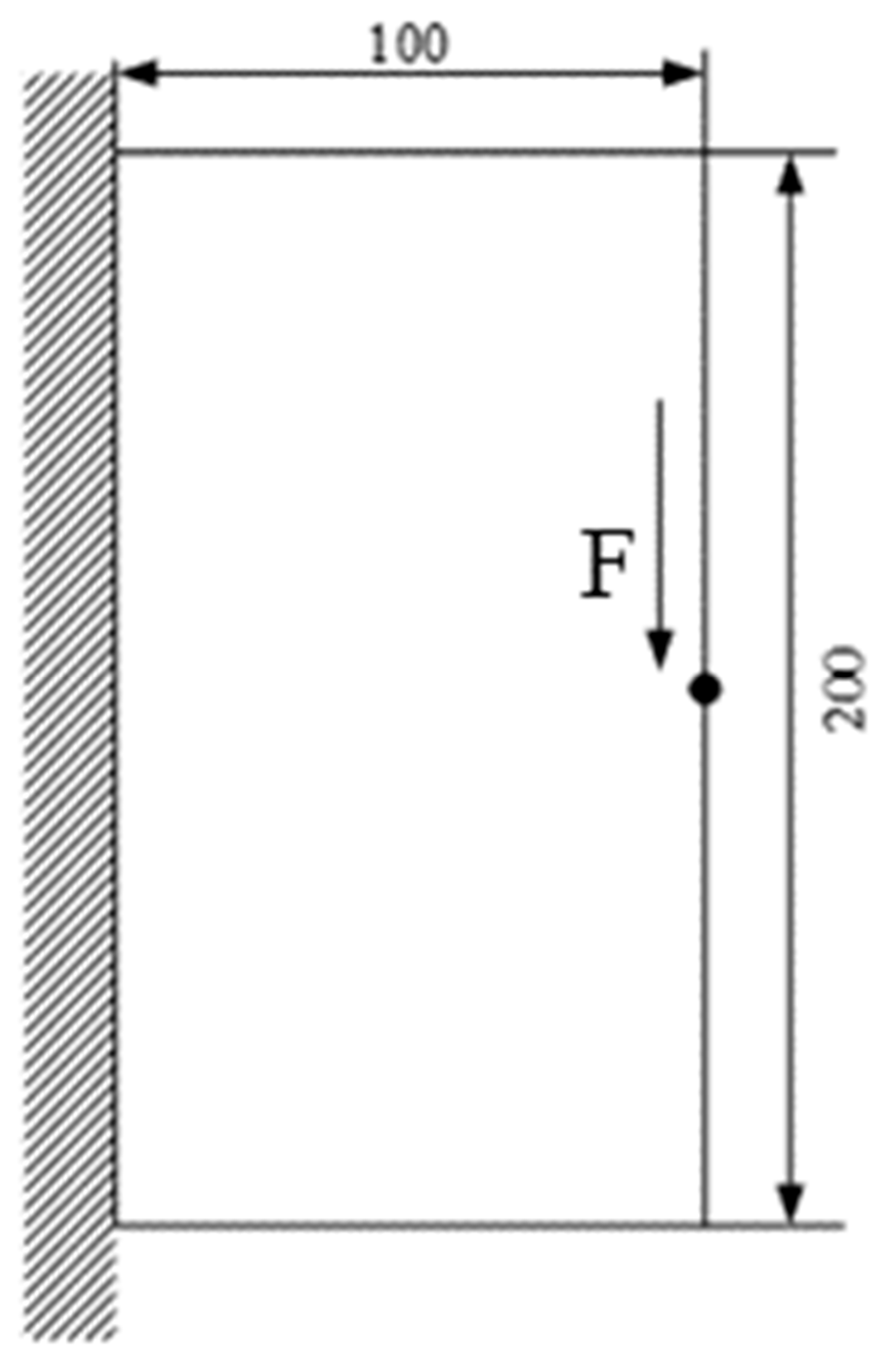
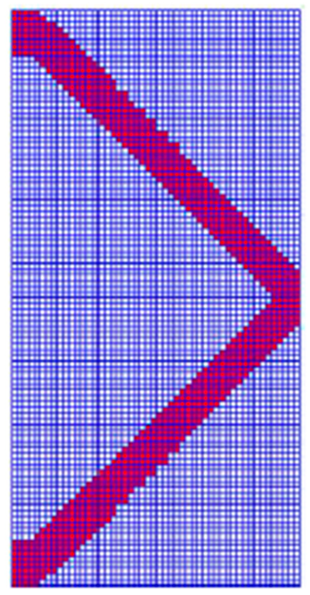
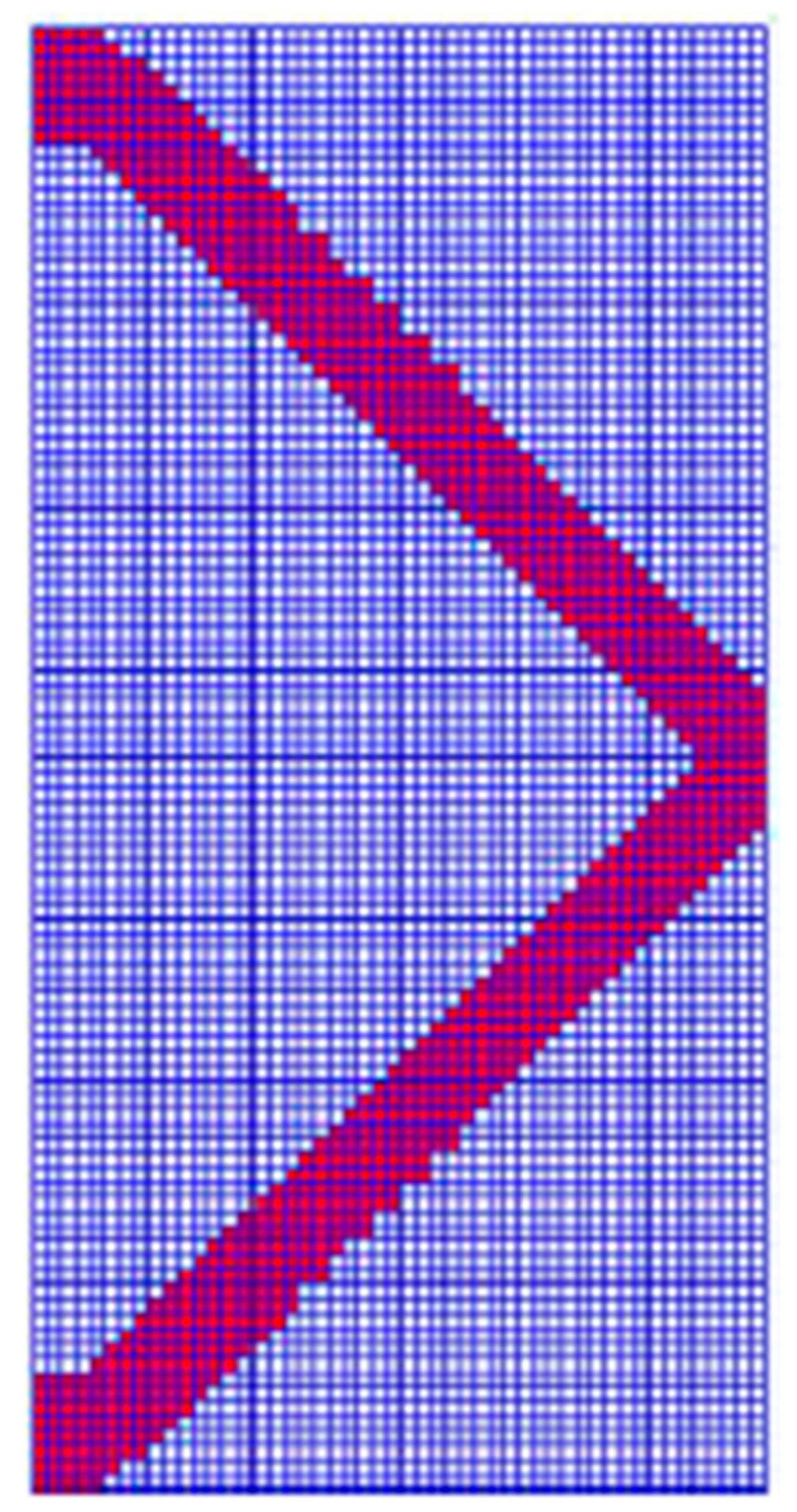
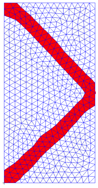
The base structure is shown in
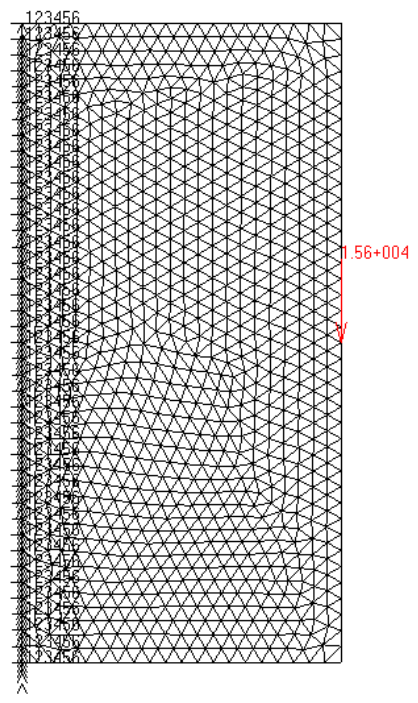
Figure 3, the corresponding finite element model is shown in
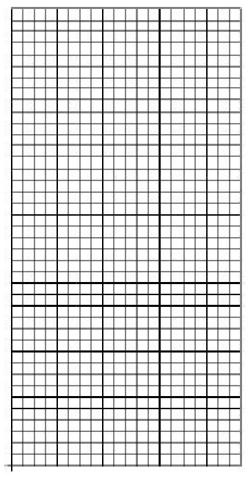
Figure 4, and the fixed background mesh is shown in
Figure 5. The structure has dimensions of 100 mm × 200 mm × 6 mm. The material has a Young’s modulus of 68.89 GPa and a Poisson’s ratio of 0.3. To enable a direct comparison with the traditional topology optimization result and the original MMSB result reported in Refs. [
29,
31], the same geometry, material parameters, boundary conditions, loading condition, and displacement constraint are adopted in this example. A concentrated load of F = 15.6 kN is applied at the midpoint of the right boundary, and the left boundary is fully fixed. The displacement constraint requires that the vertical downward displacement at the load application point be no greater than 0.5 mm. The finite element mesh uses three-node triangular elements, whereas the background mesh uses quadrilateral elements. The side length of both meshes is 5 mm, the convergence tolerance is set to 0.001, and the threshold is 0.5.
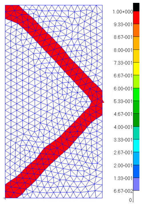
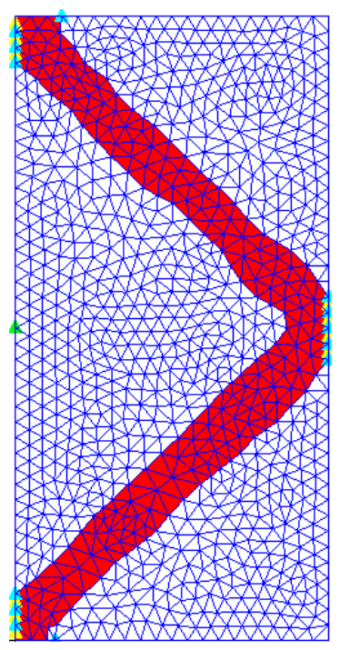
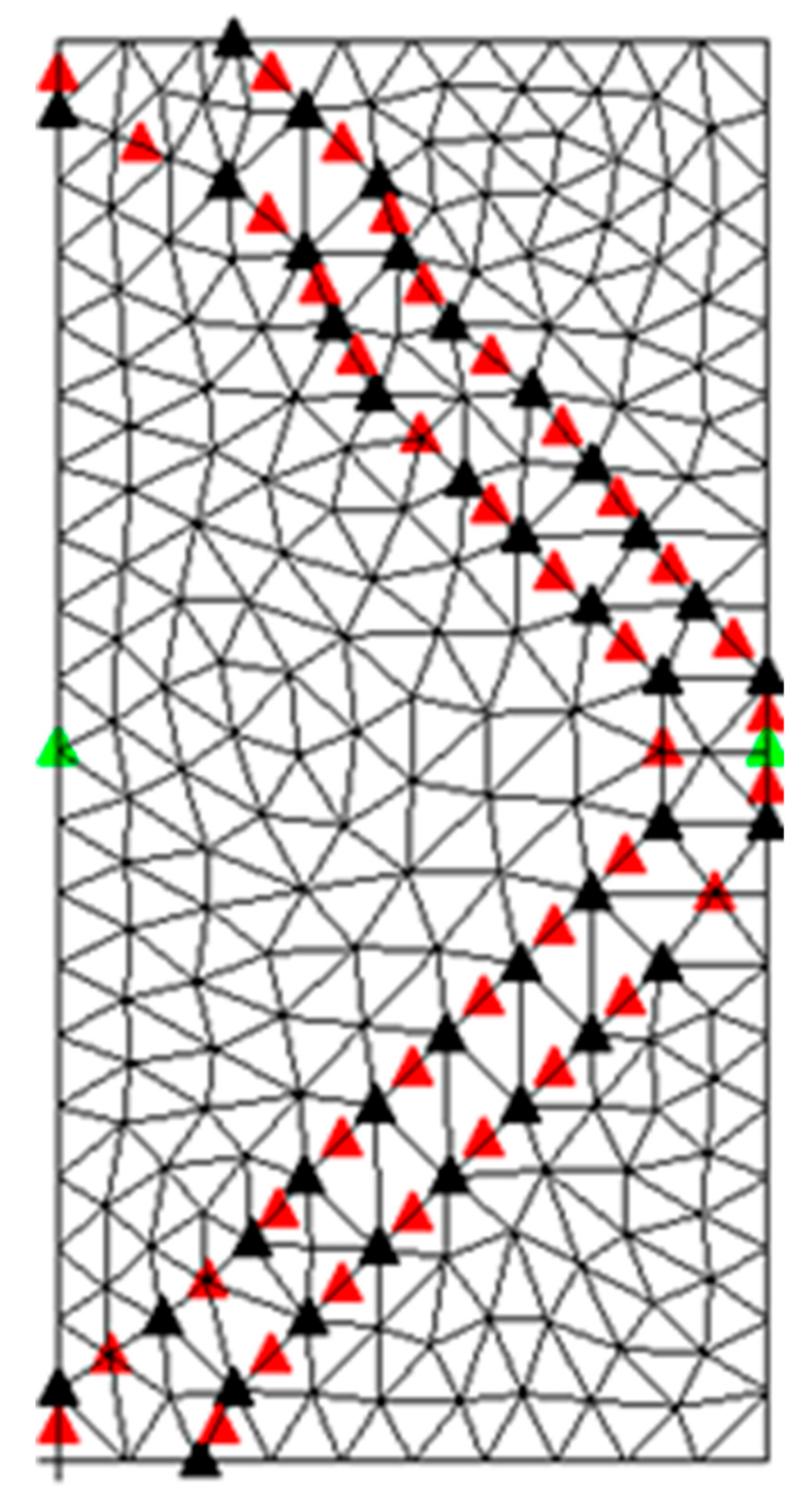
As shown in
Figure 6, the topology-variable distributions before and after each remeshing and mapping operation are consistent in the main material regions and along the load-transfer paths. No obvious shift in the main load-bearing regions or sudden change in the overall topology configuration is observed after mapping. This visual comparison suggests that the background mesh mapping procedure helps maintain the continuous evolution of topology information during remeshing.
To further quantitatively evaluate the consistency of topology-variable transfer during remeshing, a conservation check of the topology-variable field is performed. After remeshing, the element numbers, node positions, and element connectivity of the current analysis mesh change. Therefore, topology variables on the old and new current meshes cannot be directly compared through element-to-element correspondence. In this study, the weighted average topology variable is used as an overall conservation indicator to evaluate whether the topology-variable field is preserved during the mapping process.
The weighted average topology variable is defined as:
where
represents the weighted average topology variable,
is the topology variable of the
i-th element,
is the volume of the
i-th element, and
N is the total number of elements considered in the calculation.
The relative conservation error is calculated as:
where
denotes the relative conservation error,
denotes the weighted average topology variable before mapping, and
denotes the weighted average topology variable after mapping.
Example 1 is selected for this conservation check because it contains four consecutive remeshing steps and therefore provides a representative case for evaluating topology-variable transfer during repeated remeshing. Because the same background mesh mapping strategy is used in the other numerical examples, this check provides direct evidence for the effectiveness of the proposed transfer procedure.
Table 2 presents the quantitative conservation check of topology-variable transfer during the four remeshing steps in Example 1.
As shown in
Table 2, for the complete transfer process from the old current mesh to the new current mesh, the relative conservation errors from the first to fourth remeshing steps are 0.0720%, 0.3079%, 0.4648%, and 0.9774%, respectively. All these values are below 1%. This indicates that, from an overall conservation perspective, the topology-variable field is effectively preserved during the background mesh mapping procedure. Therefore, the background mesh can serve as a stable intermediate carrier for topology-variable transfer before and after remeshing, and no obvious loss of topology information is observed in this example.
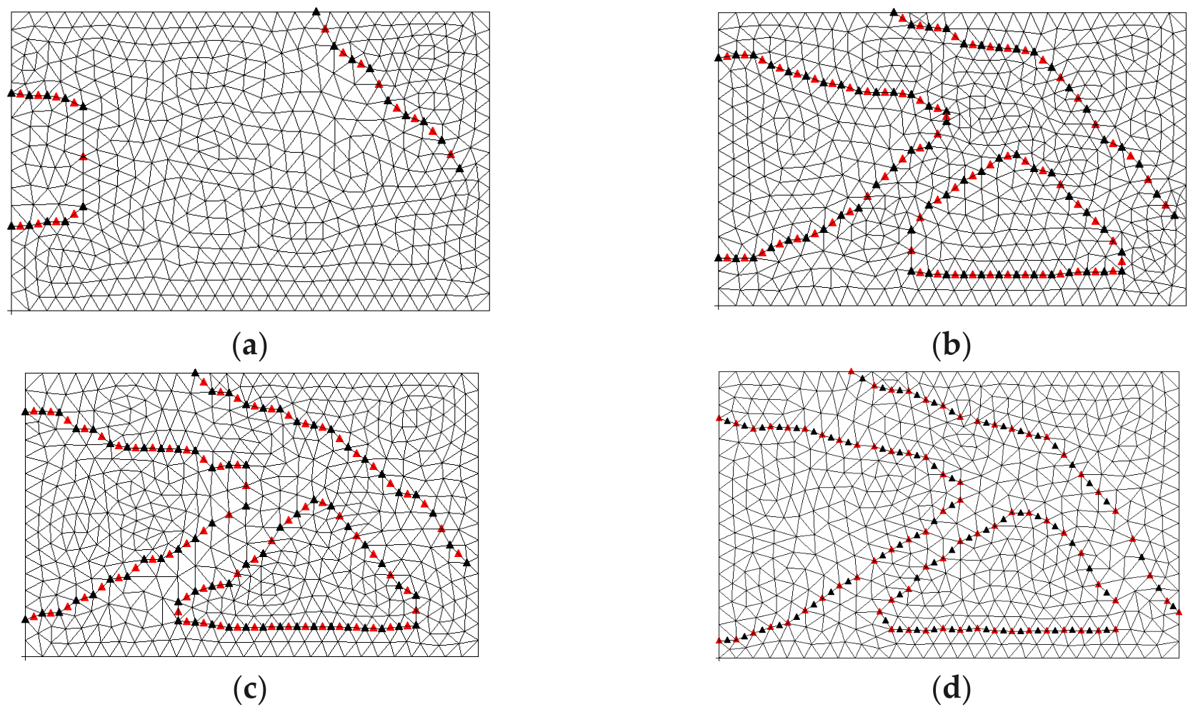
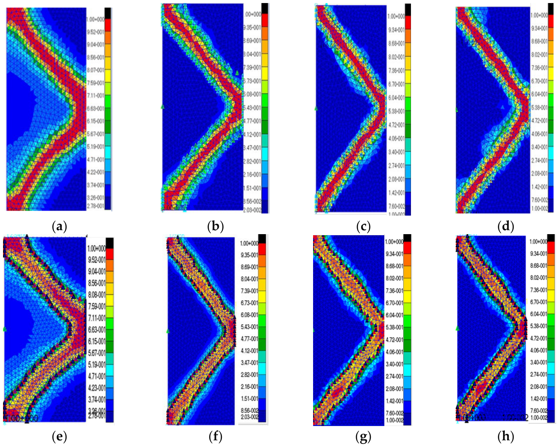
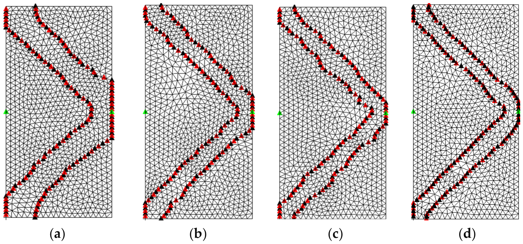
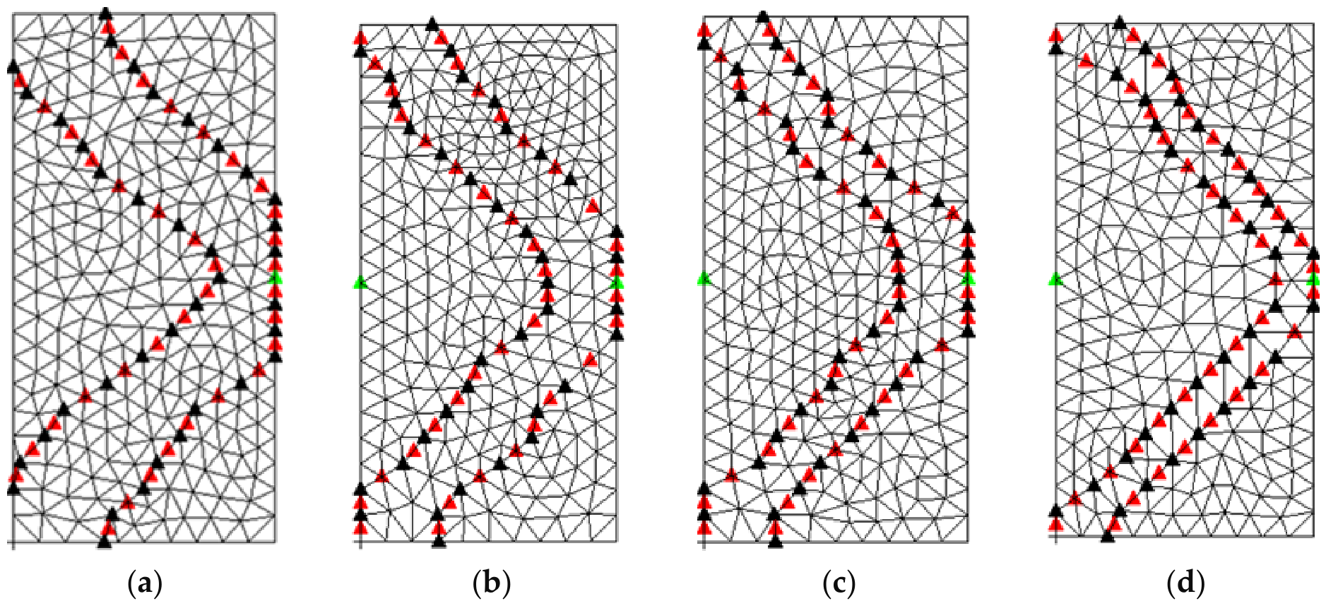
The four boundary-movement processes shown in
Figure 7 indicate that the boundary changes substantially during the first two updates and gradually stabilizes in the later stage. After the fourth boundary movement, the obtained boundary contour is relatively smooth and differs only slightly from the third result, indicating that the structural topology has essentially converged. In terms of the evolution pattern, material gradually concentrates from non-primary load-bearing regions toward the main load-bearing path and eventually forms a clear V-shaped load-bearing skeleton. This behavior reflects the redistribution of material along the main load-bearing path under the displacement constraint.
Figure 7.
Four-time boundary movement diagram in Example 1: (
a) First boundary movement; (
b) Second boundary movement; (
c) Third boundary movement; (
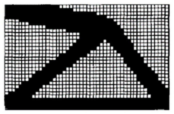
d) Fourth boundary movement. The traditional topology optimization result, the original MMSB result, and the result obtained by the improved MMSB method are shown in
Figure 8,
Figure 9 and
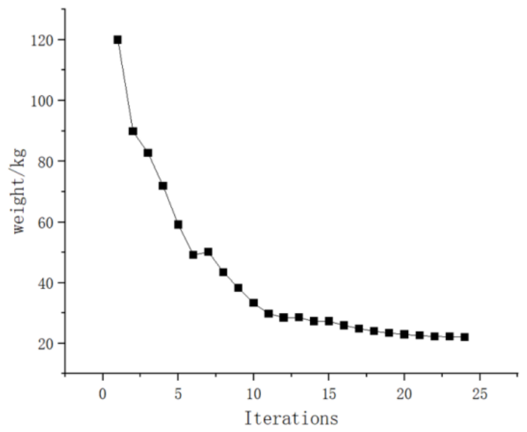
Figure 10, respectively. Combining the weight-iteration curve in
Figure 11 with the comparison results in
Table 3 shows that the improved MMSB method reduces the number of repeated result analyses while maintaining the final structural performance. Compared with the original method, the number of result analyses is reduced from 60 to 24, the number of boundary movements is reduced from 5 to 4, and the final structural weight decreases from 22.5 kg to 22.0 kg. Because the decrease in structural weight is small, the improvement of the proposed method is mainly reflected in smoother boundary representation and fewer repeated result analyses and boundary-updating operations, rather than in a significant weight-reduction advantage.
Figure 7.
Four-time boundary movement diagram in Example 1: (
a) First boundary movement; (
b) Second boundary movement; (
c) Third boundary movement; (
d) Fourth boundary movement. The traditional topology optimization result, the original MMSB result, and the result obtained by the improved MMSB method are shown in
Figure 8,
Figure 9 and
Figure 10, respectively. Combining the weight-iteration curve in
Figure 11 with the comparison results in
Table 3 shows that the improved MMSB method reduces the number of repeated result analyses while maintaining the final structural performance. Compared with the original method, the number of result analyses is reduced from 60 to 24, the number of boundary movements is reduced from 5 to 4, and the final structural weight decreases from 22.5 kg to 22.0 kg. Because the decrease in structural weight is small, the improvement of the proposed method is mainly reflected in smoother boundary representation and fewer repeated result analyses and boundary-updating operations, rather than in a significant weight-reduction advantage.

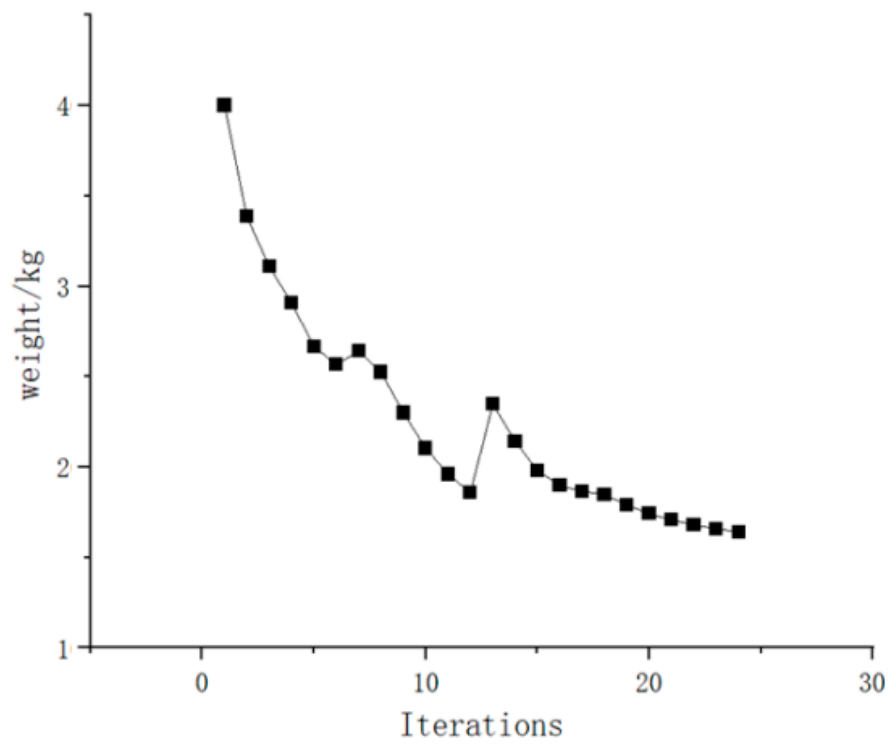
The weight-iteration curve shows that the structural weight decreases rapidly in the early stage and then gradually stabilizes. Boundary-movement and remeshing operations may cause local abrupt changes in the curve, but the overall decreasing trend is maintained. In addition, the boundary-evolution process shows that the main topology configuration does not exhibit divergent oscillation during optimization. This indicates that the proposed method maintains stable topology evolution in the presented benchmark examples.
In addition, a coarse mesh with a side length of 10 mm is used for a preliminary comparison while keeping the load, constraints, and material parameters unchanged. The results show that the improved MMSB method still produces a relatively smooth structural boundary under the coarse-mesh condition, and the main topology configuration is generally consistent with that obtained using the finer mesh. Under the same coarse-mesh condition, the traditional fixed-mesh result still exhibits obvious jagged boundaries. This comparison indicates that the proposed method can maintain its boundary-smoothing effect to some extent at a lower mesh resolution. However, this comparison is only a preliminary examination of mesh influence. A more systematic mesh-density sensitivity study with different element sizes is still needed to further evaluate convergence behavior, local finite element accuracy, and boundary-representation quality. It should also be noted that the comparison of boundary smoothness is mainly based on observed boundary morphology; no quantitative smoothness metric, such as curvature variation, boundary length, or geometric error, is introduced in the present study. The boundary-movement stages under the coarse-mesh condition are shown in
Figure 12.
The optimized boundaries obtained by the traditional method and the MMSB method with a fine mesh are shown in
Figure 13 and
Figure 14, respectively.
The topology boundary obtained after mesh thickening is shown in
Figure 15.
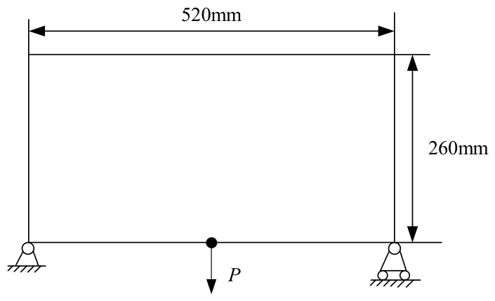
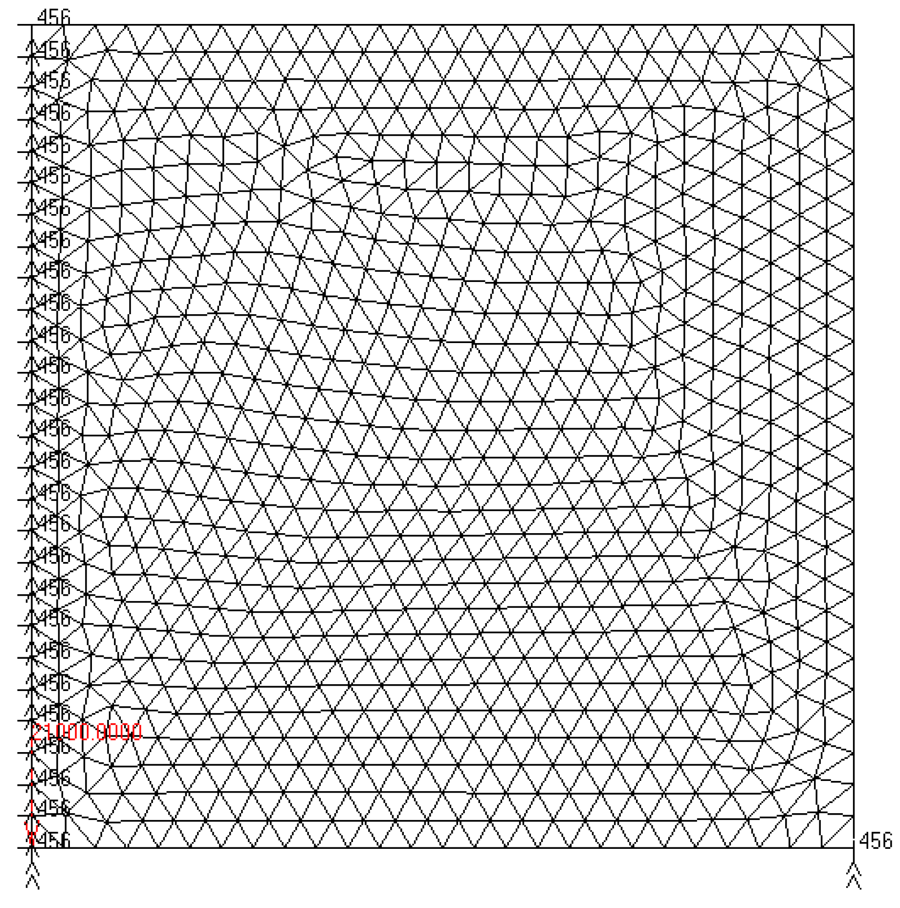
Example 2 has dimensions of 520 mm × 260 mm × 6 mm, as shown in
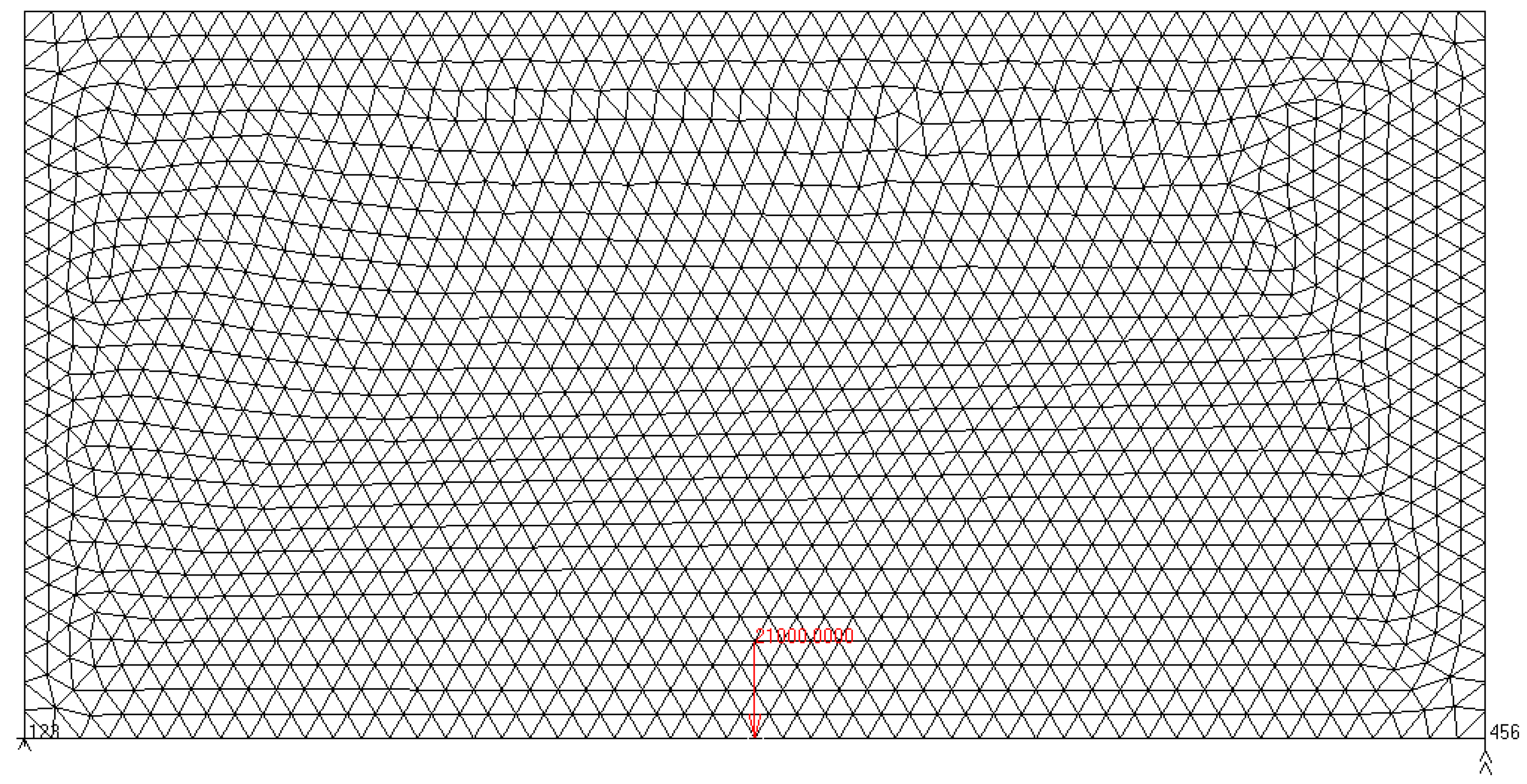
Figure 16. The symmetric basic structure, the finite element model of the basic structure, and the simplified finite element model are shown in
Figure 17,
Figure 18 and
Figure 19, respectively. To enable a direct comparison with the traditional topology optimization result and the original MMSB result reported in Refs. [
21,
31], the same geometry, material parameters, boundary conditions, loading condition, and displacement constraint are adopted. The material has a Young’s modulus of 68.89 GPa and a Poisson’s ratio of 0.3. A concentrated load of P = 21 kN is applied at the left endpoint of the lower boundary, while the left boundary and the lower-right corner are simply supported. The displacement constraint requires that the vertical downward displacement at the load application point be no greater than 0.8 mm. Three-node triangular elements are adopted; the element side length is 10 mm, the convergence tolerance is set to 0.001, and the threshold is 0.5.
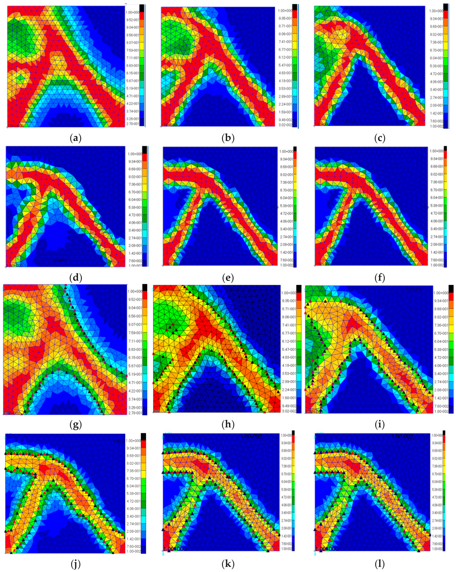
As shown in
Figure 20, although many local features and internal voids are formed during optimization, the topology-variable distributions before and after remeshing remain generally consistent in the main material regions. After mapping, the high-value regions are still concentrated near the main load-bearing regions, and no obvious topology fracture or sudden feature shift is observed. This visual comparison indicates that the background mesh mapping procedure can support continuous topology-information evolution even for more complex topology configurations.
The structural evolution in Example 2 exhibits clear stages. In the initial stage, the material distribution is relatively broad, and the internal load-bearing skeleton is not yet fully defined. As the iteration proceeds, the material gradually concentrates along the main load-bearing paths, and stable cross supports and peripheral load-bearing boundaries begin to form inside the structure. In the later stage, the topology configuration is essentially established. The topology-variable distributions before and after grid mapping in Example 2 are compared in
Figure 20.
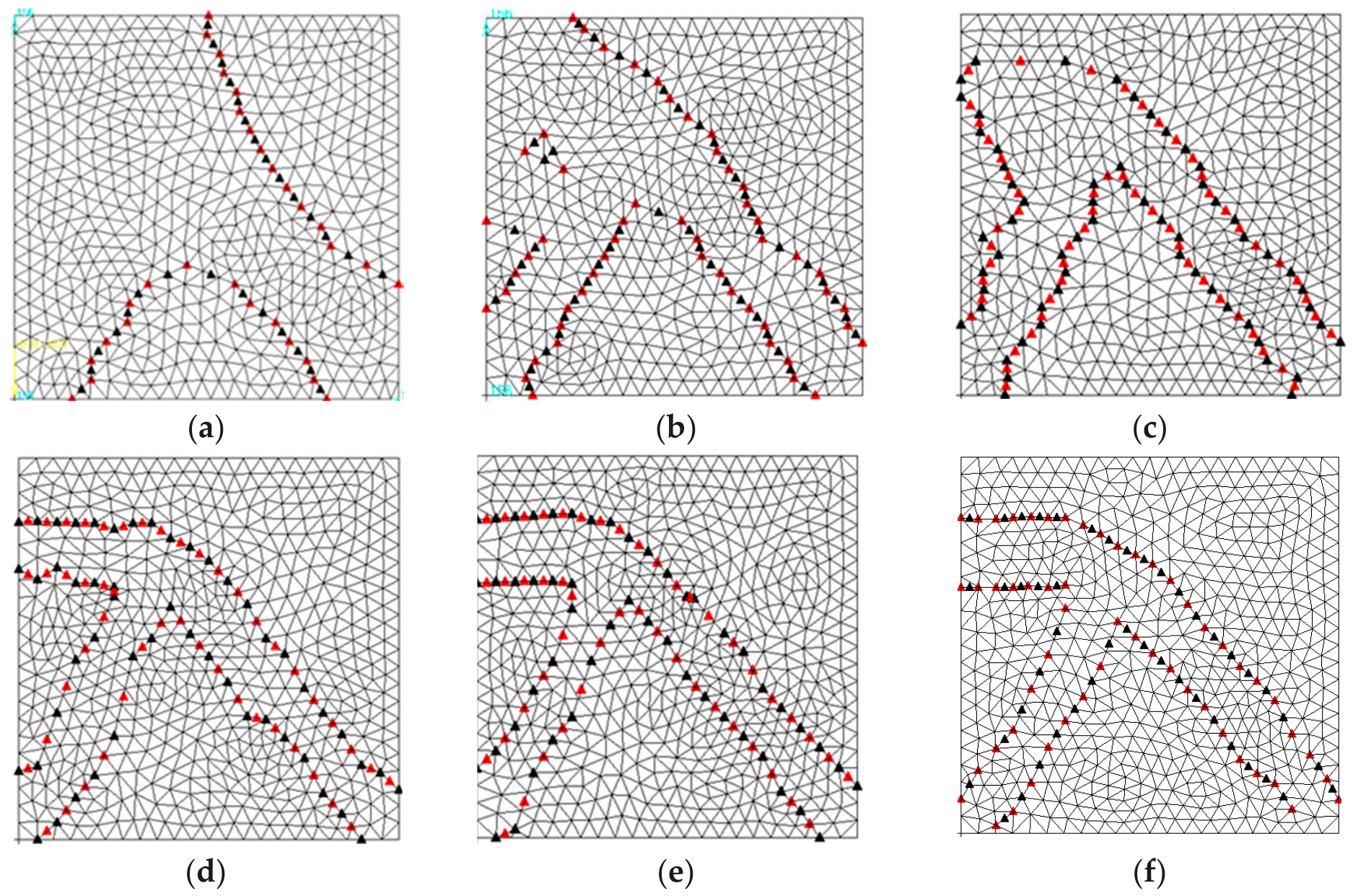
The six boundary-movement stages in Example 2 are shown in
Figure 21. The topology configuration obtained by traditional topology optimization in Example 2 is shown in
Figure 22.
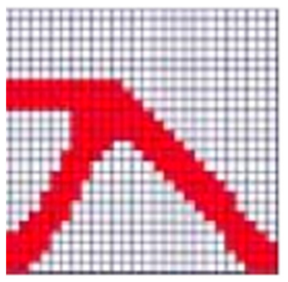
The final topology configuration obtained by the original MMSB method is shown in
Figure 23. The optimized boundary obtained by the improved MMSB method is shown in
Figure 24.
Figure 24.
Topology configuration obtained by the improved MMSB method in Example 2. The weight-iteration curve for the six boundary movements in Example 2 is shown in
Figure 25.
Figure 24.
Topology configuration obtained by the improved MMSB method in Example 2. The weight-iteration curve for the six boundary movements in Example 2 is shown in
Figure 25.
The improved MMSB method also requires fewer repeated result analyses in this example. The original MMSB method requires 8 boundary movements and 144 result analyses to complete the calculation, whereas the improved method requires only 6 boundary movements and 36 result analyses to reach convergence. Meanwhile, both methods produce the same final structural weight of 101.4 kg. This indicates that the improved method reduces repeated analyses and boundary-updating operations without changing the final structural weight. Therefore, in this example, the engineering significance of the proposed method is mainly reflected in maintaining comparable structural performance while improving boundary clarity and topology-evolution continuity.
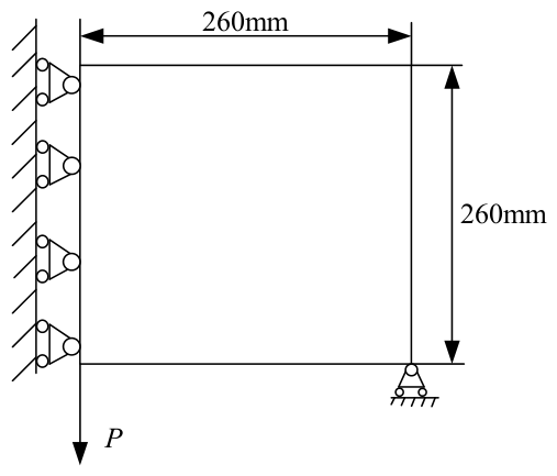
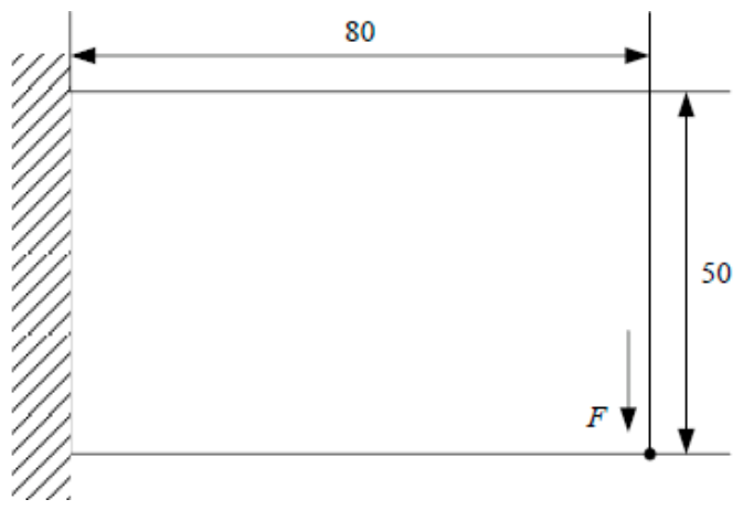
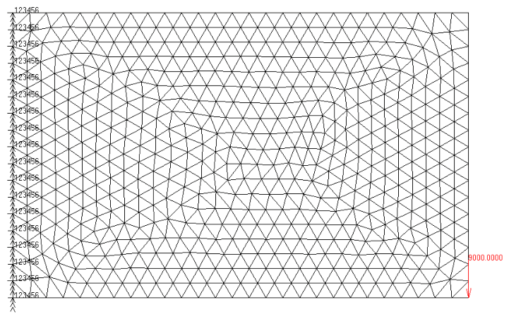
Example 3 has dimensions of 80 mm × 50 mm × 1 mm, as shown in
Figure 26, and its finite element model is shown in
Figure 27. To maintain consistency with the traditional topology optimization result and the original MMSB result reported in Refs. [
20,
31], the same geometry, material parameters, boundary condition, loading condition, and displacement constraint are adopted. The material has a Young’s modulus of 1.0 × 10
6 MPa and a Poisson’s ratio of 0.3. A concentrated load of
F = 9000 N is applied at the lower-right corner of the model, while the left boundary is fixed. The displacement constraint requires that the vertical downward displacement at the load application point be no greater than 0.5 mm. Three-node triangular elements are adopted; the element side length is 10 mm, the convergence tolerance is set to 0.001, and the threshold is 0.5.
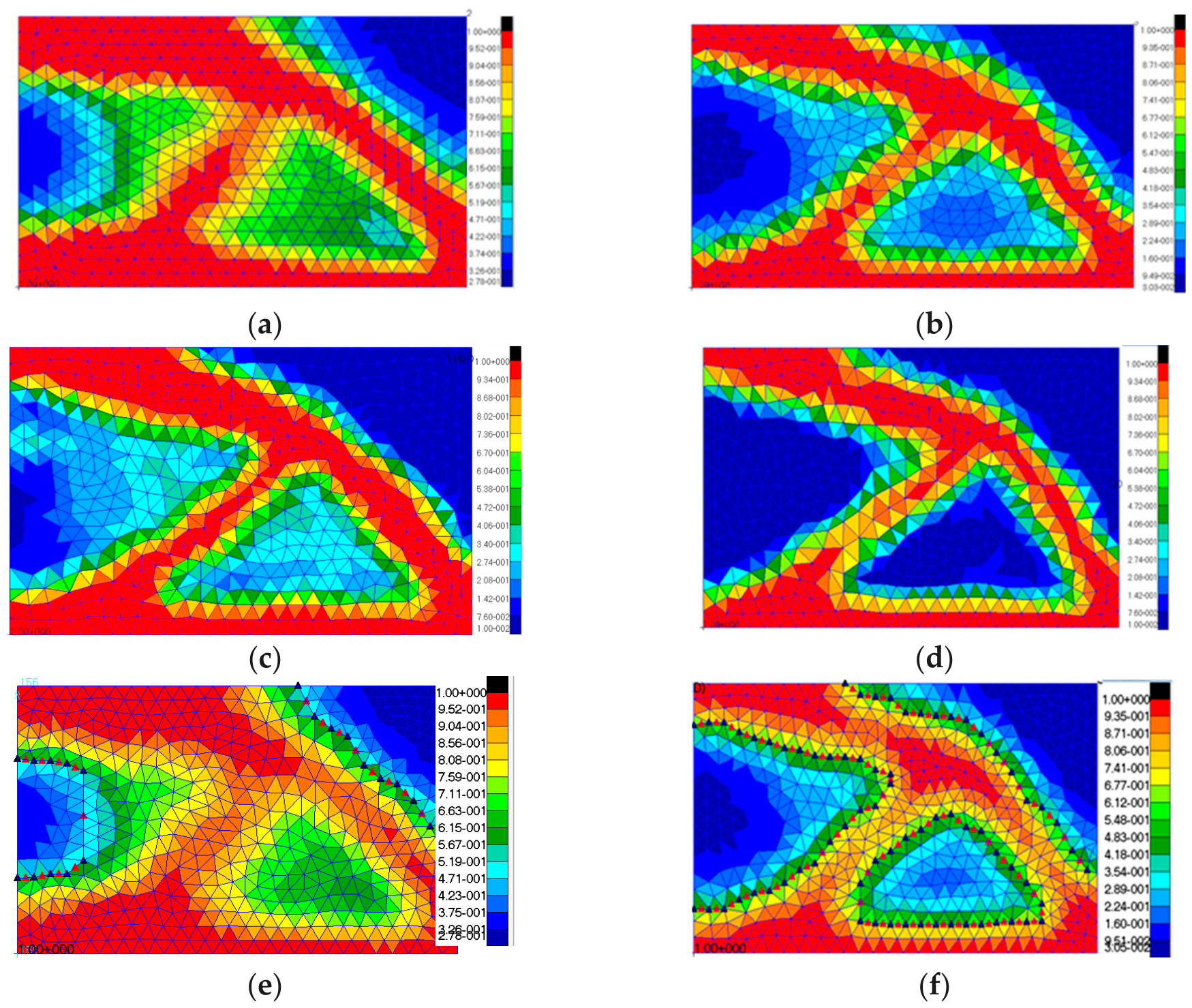
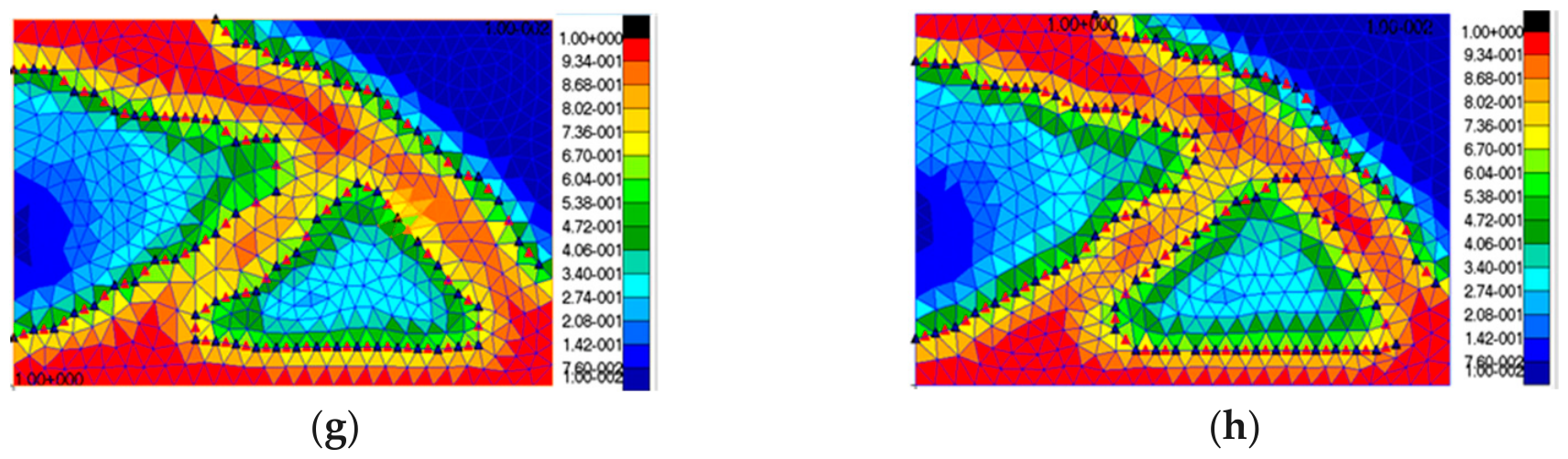
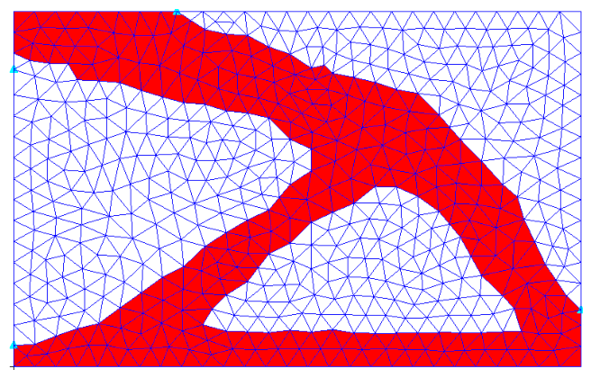
It should be noted that the element size used in this example is relatively coarse compared with the overall dimensions of the structure. Because the design domain is small, some local members are represented by only a limited number of elements. Therefore, local thickness transitions and finite element accuracy in these regions may be affected by mesh density. This example is mainly used to compare the proposed method with the traditional topology optimization result and the original MMSB result under the same benchmark conditions. For more accurate local structural evaluation, especially in thin-member regions, a finer mesh should be adopted in future studies. According to the four boundary-movement processes, the structural boundary changes noticeably in the early updates. By the fourth movement, the boundary contour becomes relatively smooth and changes only slightly compared with the third result, indicating structural convergence. In the final topology, material is mainly retained in the key load-bearing regions connecting the support end and the load application point, whereas regions with smaller contributions to the overall stiffness are gradually removed. This is consistent with the general behavior of displacement-constrained problems, in which material is retained along the main load-bearing paths. The topology-variable distributions before and after mesh mapping in Example 3 are compared in
Figure 28.
The four boundary-movement stages in Example 3 are shown in
Figure 29.
The topology configuration obtained by traditional topology optimization is shown in
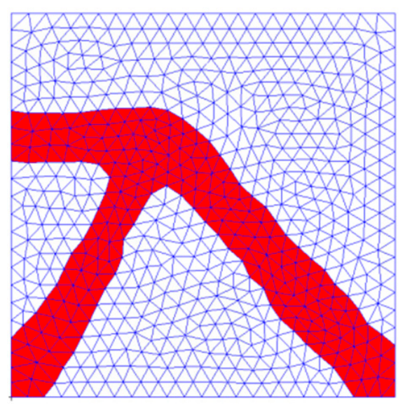
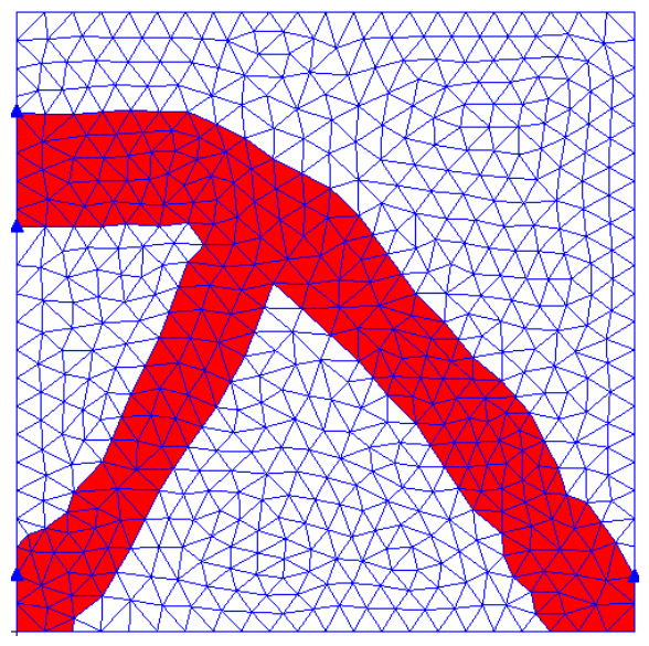
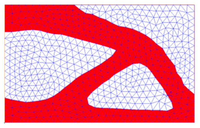
Figure 30. The final topology configuration obtained by the original MMSB method and the topology configuration obtained by the improved MMSB method are shown in
Figure 31 and
Figure 32, respectively.
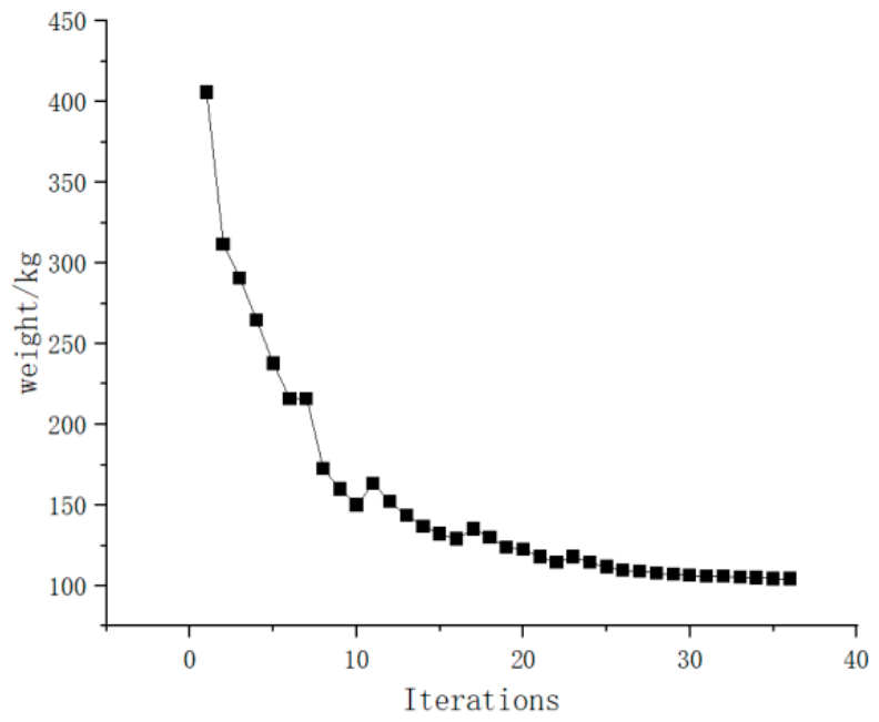
The weight-iteration curve for four boundary movements in Example 3 is shown in
Figure 33.
Compared with the original MMSB method, the improved method reduces the number of result analyses from 112 to 24 and the number of boundary movements from 7 to 4. The final structural weight is 1.64 kg, which is close to the 1.65 kg obtained by the original method. The small difference in structural weight should not be interpreted as a significant weight-reduction advantage. These results indicate that the improved method reduces repeated result analyses and boundary-updating operations while maintaining the main optimization result and a smooth-boundary representation.
To clarify the relationship between the reduction in result analyses and the final optimization performance, the results in
Table 3,
Table 4 and
Table 5 are considered together with the displacement-constraint verification in
Table 6.
Table 3,
Table 4 and
Table 5 compare the original MMSB method and the improved MMSB method in terms of the number of result analyses, structural weight, and boundary movements for the three numerical examples. These results show that the improved MMSB method reduces repeated result analyses and boundary movements, while the final structural weights remain close to those obtained by the original MMSB method.
However, reducing the number of result analyses alone is not sufficient to evaluate the final design quality. Therefore, the displacement responses at the constrained points are further summarized in
Table 6. This additional verification examines whether the optimized structures obtained by the improved MMSB method still satisfy the prescribed displacement constraints after the reduction in repeated analyses and boundary movements.
As shown in
Table 6, the final displacement values of the optimized structures in the three numerical examples are all lower than the corresponding allowable limits. Specifically, the final displacements of Examples 1–3 are 0.4730 mm, 0.7781 mm, and 0.4996 mm, respectively, while the corresponding allowable displacement limits are 0.5 mm, 0.8 mm, and 0.5 mm. The corresponding violation ratios are −5.40%, −2.74%, and −0.08%, respectively. Because all violation ratios are negative, the prescribed displacement constraints are satisfied in all three numerical examples.
Combining the results in
Table 3,
Table 4,
Table 5 and
Table 6 shows that the improved MMSB method reduces the number of result analyses and boundary movements in all three examples, while the final structural weights remain comparable to those obtained by the original MMSB method. In addition, all final displacement values satisfy the prescribed displacement constraints. These results indicate that the reduction in repeated result analyses and boundary-updating operations does not cause an obvious deterioration of the final structural performance in the present examples. Therefore, the improvement of the proposed method should be understood more specifically as a reduction in repeated analyses and boundary movements while maintaining comparable final design performance, rather than as a directly measured reduction in total CPU time.
5. Conclusions
This study establishes a continuum topology optimization model based on the ICM method, with structural weight minimization as the objective and displacement as the constraint. To address the jagged-boundary problem in traditional fixed-mesh topology optimization, an improved MMSB method is proposed by introducing holographic scanning and background mesh mapping into the original MMSB framework. In the proposed method, a triangular mesh is used as the current analysis mesh. During optimization, threshold isocontours are extracted, and remeshing is performed along these contours. In this way, the structural boundary is gradually updated and reconstructed, leading to topological configurations with clearer boundary representations.
The numerical results show that the improved MMSB method can alleviate the jagged-boundary problem commonly observed in traditional fixed-mesh topology optimization. The topology-variable distributions before and after remeshing show good consistency in the main material regions and load-transfer paths. Compared with the original MMSB method, the proposed method reduces the number of result analyses from 60 to 24, from 144 to 36, and from 112 to 24 in the three numerical examples, respectively. The number of boundary movements is also reduced from 5 to 4, from 8 to 6, and from 7 to 4, respectively. Meanwhile, the final structural weights remain close to those obtained by the original MMSB method, and the final displacement responses satisfy the prescribed displacement constraints in all examples. These results indicate that the reduction in repeated result analyses and boundary-updating operations does not lead to an obvious deterioration of the final structural performance in the present examples. Because total CPU time is not used as a controlled comparison indicator in this study, the improvement of the proposed method should be understood as a reduction in repeated result analyses and boundary movements under the same benchmark conditions, rather than as a directly measured reduction in total computational time.
Nevertheless, the present study still has some limitations. First, the numerical verification is mainly based on two-dimensional examples. Although the proposed framework can, in principle, be extended to three-dimensional continuum topology optimization, such an extension would involve additional difficulties, including boundary-surface extraction from three-dimensional topology-variable fields, surface and volume remeshing, topology-variable transfer between different three-dimensional meshes, and increased computational and storage requirements. Second, the influence of mesh density is examined only preliminarily, and a more systematic sensitivity analysis with different element sizes is still needed. Third, although a quantitative conservation check of topology-variable transfer has been added in the revised manuscript, more comprehensive mapping-error evaluation and objective boundary-smoothness assessment are still needed. In future work, more comprehensive quantitative mapping-error evaluation, boundary smoothness metrics, mesh-sensitivity analysis, and comparisons with other smooth-boundary topology optimization approaches, such as level-set-based methods, MMC-based methods, and post-processing-based smoothing strategies, will be investigated to more comprehensively evaluate the applicability and limitations of the proposed method.