Algebraic Combinatorics in Financial Data Analysis: Modeling Sovereign Credit Ratings for Greece and the Athens Stock Exchange General Index

Abstract

This study investigates the relationship between sovereign credit rating transitions and domestic equity market performance, focusing on Greece from 2004 to 2024. Although credit ratings are central to sovereign risk assessment, their immediate influence on financial markets remains contested. This research adopts a multi-method analytical framework combining algebraic combinatorics and time-series econometrics. The methodology incorporates the construction of a directed credit rating transition graph, the partially ordered set representation of rating hierarchies, rolling-window correlation analysis, Granger causality testing, event study evaluation, and the formulation of a reward matrix with optimal rating path optimization. Empirical results indicate that credit rating announcements in Greece exert only modest short-term effects on the Athens Stock Exchange General Index, implying that markets often anticipate these changes. In contrast, sequential downgrade trajectories elicit more pronounced and persistent market responses. The reward matrix and path optimization approach reveal structured investor behavior that is sensitive to the cumulative pattern of rating changes. These findings offer a more nuanced interpretation of how sovereign credit risk is processed and priced in transparent and fiscally disciplined environments. By bridging network-based algebraic structures and economic data science, the study contributes a novel methodology for understanding systemic financial signals within sovereign credit systems.

1. Introduction

The increasing complexity and interconnectivity of global financial systems necessitate the development of novel analytical frameworks capable of elucidating both the structural and dynamic properties of financial phenomena. Once confined to the realm of pure mathematics, algebraic combinatorics has recently found fertile ground in the domains of data science [1,2] and financial optimization [3]. The evolution of combinatorics in financial modeling has progressed well beyond its early applications in elementary probability, giving rise to sophisticated combinatorial structures and algorithms that now underpin modern financial decision-making processes. Originally employed to compute probabilities—such as estimating the likelihood of specific portfolio outcomes through combinations of financial ratios—combinatorics has since expanded into data-intensive fields including big data analytics and machine learning, where combinatorial techniques play a pivotal role in scenario generation and pattern recognition [4].

Among these tools, graph theory has emerged as a foundational methodology, offering a powerful framework for representing and analyzing the intricate network of interactions that characterize financial systems [5]. Graph-theoretic models have been instrumental in quantifying systemic risk, analyzing the propagation of financial contagion, and revealing latent market structures. Notably, models such as those proposed by [6] have proven particularly effective in capturing interbank exposures and the cascading effects of credit interdependencies. The formalism of graph theory enables a rigorous exploration of financial network stability under conditions of systemic stress.

In parallel, combinatorial optimization has become integral to portfolio construction, asset allocation and risk assessment. Techniques such as integer programming and dynamic programming are frequently employed to solve high-dimensional optimization problems in portfolio management [7], while discrete-time models like binomial trees and lattice structures continue to underpin option pricing and risk-neutral valuation methodologies [8]. Combinatorial methods have also contributed significantly to the optimization of algorithmic trading systems and order book structures, thereby enhancing the operational efficiency and robustness of automated financial strategies.

A particularly promising frontier lies at the intersection of combinatorics and machine learning, most notably through the development of graph neural networks (GNNs). GNNs have demonstrated strong capabilities in learning from graph-structured data, offering improved predictions of complex system behaviors and enabling the optimization of intricate financial processes [9]. Recent advances in this area have further highlighted their potential to serve as scalable solvers for otherwise intractable combinatorial optimization problems in financial contexts.

Traditionally, the modeling of credit rating dynamics has relied on Markov chains, which are based on the assumption that future states depend exclusively on current states [10]. While useful for certain applications, Markovian approaches can obscure higher-order dependencies and overlook deeper structural features of rating movements [11]. To address these limitations, algebraic combinatorics has introduced more expressive mathematical representations, such as partially ordered sets or “posets”, chains, antichains, and lattices [12,13]. These structures facilitate the classification of economic agents and the modeling of preference hierarchies, enabling a more nuanced understanding of financial systems.

Emerging research has begun to apply poset-based methods to financial networks, offering new insights into how economic hierarchies can be formalized and analyzed [14]. However, the direct application of algebraic combinatorics for modeling sovereign credit ratings and their empirical relationship with equity market performance remains an under-explored area. This gap underscores the need for integrative approaches that connect combinatorial mathematics with financial datasets to uncover latent structures and dynamics related to credit risk and investor sentiment.

Motivated by this perspective, the present study investigates the impact of sovereign credit rating transitions on equity market performance. Specifically, it explores the utility of algebraic combinatorics in modeling credit rating movements and their relationship with the Athens Stock Exchange General Index (ASE Index), a prominent financial benchmark for the Greek economy. Credit ratings, such as those issued by Moody’s, represent ordinal measures of creditworthiness and are widely recognized for their influence on borrowing costs, investment flows, and macroeconomic policymaking [15]. Changes in these ratings—including upgrades, downgrades, and shifts in outlook—can have pronounced effects on market dynamics [16], making their structural behavior highly relevant for both risk management and economic forecasting. Figure 1 presents a simplified credit rating transition graph designed to illustrate the basic mechanics of rating changes. The diagram consists of three credit quality levels—A (high), B (moderate), and C (low)—positioned vertically to reflect their ordinal hierarchy. Arrows indicate possible transitions between ratings: red arrows on the right represent downgrades, such as those caused by fiscal deterioration or debt crises (e.g., A to B or B to C), while green arrows on the left denote upgrades resulting from reforms or economic recovery (e.g., C to B or B to A).

The ASE Index serves as a proxy for investor sentiment and macroeconomic confidence in Greece. Over the past three decades, the Greek economy has experienced substantial volatility, including a sovereign debt crisis, the implementation of austerity measures, and an extended period of economic stagnation and recovery [17]. The nation’s credit rating history, as documented by Moody’s, reflects this economic turbulence and thus offers a rich empirical basis for combinatorial modeling. By integrating algebraic structures with empirical financial data, this research aims to advance both the theoretical understanding and practical applications of combinatorics in the analysis of sovereign credit risk and its market consequences.

The objective of this study is to investigate the relationship between sovereign credit rating transitions and domestic equity market performance, using Greece as a case study over the period 2004–2024. For this reason, we employed a multi-method framework that includes directed graph modeling, rolling-window correlation analysis, Granger causality tests, event studies, and a reward matrix approach. The central goal is to assess whether rating changes convey new information to markets or merely formalize expectations already priced in. Furthermore, we seek to identify whether market reactions are more strongly associated with isolated rating shifts or with cumulative transition paths. By integrating tools from network theory and econometric analysis, this research contributes to a more nuanced understanding of credit ratings’ informational value and market signaling power. The results are intended to inform policymakers, investors, and credit rating agencies on the structural dynamics of sovereign risk perception.

Our findings reveal that sovereign credit rating transitions in Greece have a limited immediate impact on the domestic equity market, suggesting that such announcements are often anticipated by investors. Granger causality tests show no strong predictive relationship between ratings and market movements, while the event study indicates modest abnormal returns around significant rating changes. However, the reward matrix and optimal path analysis highlight that sequential rating transitions, rather than isolated events, elicit more pronounced market responses. These results emphasize the importance of structural downgrade trajectories in shaping investor sentiment and risk assessment in mature financial systems. This research is among the first to apply algebraic combinatorics to empirically model sovereign rating dynamics and their equity market implications.

The rest of the manuscript is organized as follows. Section 2 presents the data sources, the ordinal transformation of Moody’s credit ratings, and the analytical framework. Section 3 reports the empirical results, and Section 4 offers a discussion of the results, limitations, and future research. Section 5 concludes the paper, summarizing the main contributions and highlighting methodological innovations.

2. Materials and Methods

This section outlines the analytical framework used to examine the dynamic interactions between sovereign credit ratings and financial market performance in Greece over the period 2004–2024.

2.1. Data Description and Preprocessing

Moody’s Investors Service [18] assigns sovereign credit ratings to assess a government’s ability and willingness to meet its debt obligations in a timely manner. These ratings reflect the relative credit risk of sovereign issuers and are expressed on an ordinal scale ranging from Aaa, indicating the highest quality and lowest credit risk, to C, denoting extremely speculative obligations and a high likelihood of default (

Table 1. Moody’s sovereign credit ratings.

No.	Rating	Meaning
1	Aaa	Highest quality, minimal credit risk
2	Aa1	High quality, very low credit risk (upper end of Aa)
3	Aa2	High quality, very low credit risk (mid-range of Aa)
4	Aa3	High quality, very low credit risk (lower end of Aa)
5	A1	Upper-medium grade, low credit risk (upper end of A)
6	A2	Upper-medium grade, low credit risk (mid-range of A)
7	A3	Upper-medium grade, low credit risk (lower end of A)
8	Baa1	Medium grade, moderate credit risk (upper end of Baa)—lowest investment grade
9	Baa2	Medium grade, moderate credit risk (mid-range of Baa)
10	Baa3	Medium grade, moderate credit risk (lower end of Baa)—borderline investment grade
11	Ba1	Speculative, substantial credit risk (upper end of Ba)
12	Ba2	Speculative, substantial credit risk (mid-range of Ba)
13	Ba3	Speculative, substantial credit risk (lower end of Ba)
14	B1	Highly speculative, high credit risk (upper end of B)
15	B2	Highly speculative, high credit risk (mid-range of B)
16	B3	Highly speculative, high credit risk (lower end of B)
17	Caa1	Poor standing, very high credit risk (upper end of Caa)
18	Caa2	Poor standing, very high credit risk (mid-range of Caa)
19	Caa3	Poor standing, very high credit risk (lower end of Caa)
20	Ca	Highly speculative, likely in or near default
21	C	Lowest rating, typically in default with little prospect for recovery

). The rating process integrates both quantitative and qualitative assessments. Quantitatively, Moody’s considers macroeconomic indicators such as GDP growth, fiscal and current account balances, inflation, and external debt sustainability. Qualitatively, the agency evaluates institutional strength, policy credibility, governance effectiveness, and geopolitical risks. Ratings are determined by Moody’s Sovereign Risk Group through a structured framework that weighs economic strength, institutional quality, fiscal strength, and susceptibility to event risk. Importantly, sovereign ratings are not static but subject to continuous monitoring and periodic review. They may be placed on review for upgrade or downgrade, or assigned a rating outlook, indicating the likely direction of future changes. These ratings serve as critical inputs for global capital markets, influencing investor behavior, borrowing costs, and international policy decisions.

Credit ratings are originally expressed in alphanumeric format (e.g., A1, Ba3), reflecting ordinal assessments of creditworthiness. For the purposes of this analysis, each rating was systematically converted into an integer scale ranging from 1 (corresponding to Aaa, the highest rating) to 21 (corresponding to C, the lowest rating). This transformation facilitates quantitative analysis, enables the application of mathematical and statistical techniques, and supports the construction of graph-based models. Let the set of Moody’s credit ratings ${\mathrm{R}\mathrm{a}\mathrm{t}\mathrm{i}\mathrm{n}\mathrm{g}\_\mathrm{L}\mathrm{a}\mathrm{b}\mathrm{e}\mathrm{l}}_{\mathrm{t}}=\left\{\mathrm{A}\mathrm{a}\mathrm{a},\mathrm{A}\mathrm{a}1,\dots ,\mathrm{C}\right\}$ be mapped to a totally ordered numerical scale ${\mathrm{R}\mathrm{a}\mathrm{t}\mathrm{i}\mathrm{n}\mathrm{g}\_\mathrm{I}\mathrm{n}\mathrm{t}\mathrm{e}\mathrm{g}\mathrm{e}\mathrm{r}}_{\mathrm{t}}=\left\{\mathrm{1,2},\dots ,21\right\}$, where a bijective function $\mathrm{f}:{\mathrm{R}\mathrm{a}\mathrm{t}\mathrm{i}\mathrm{n}\mathrm{g}\_\mathrm{L}\mathrm{a}\mathrm{b}\mathrm{e}\mathrm{l}}_{\mathrm{t}}\to {\mathrm{R}\mathrm{a}\mathrm{t}\mathrm{i}\mathrm{n}\mathrm{g}\_\mathrm{I}\mathrm{n}\mathrm{t}\mathrm{e}\mathrm{g}\mathrm{e}\mathrm{r}}_{\mathrm{t}}$ assigns a unique integer to each rating level based on its credit quality, such that

$${\mathrm{R}\mathrm{a}\mathrm{t}\mathrm{i}\mathrm{n}\mathrm{g}\_\mathrm{I}\mathrm{n}\mathrm{t}\mathrm{e}\mathrm{g}\mathrm{e}\mathrm{r}}_{\mathrm{t}}=\mathrm{f}\left({\mathrm{R}\mathrm{a}\mathrm{t}\mathrm{i}\mathrm{n}\mathrm{g}\_\mathrm{L}\mathrm{a}\mathrm{b}\mathrm{e}\mathrm{l}}_{\mathrm{t}}\right),\hspace{1em}\mathrm{f}:\left\{\mathrm{A}\mathrm{a}\mathrm{a},\mathrm{A}\mathrm{a}1,\dots ,\mathrm{C}\right\}\to \left\{\mathrm{1,2},\dots ,21\right\}$$

(1)

This transformation allows ordinal categorical ratings to be embedded in a numerical framework suitable for statistical analysis and graph construction. While the transformation of Moody’s alphanumeric credit ratings into an ordinal integer scale enables the application of quantitative methods, it is important to emphasize that this encoding preserves only the ordinal properties of the data, not its cardinal meaning. Specifically, the numerical values assigned to the rating categories (e.g., Aaa = 1, C = 21) reflect a strict ranking of creditworthiness, whereby lower integers correspond to higher credit quality. However, the intervals between successive ratings are not uniformly meaningful in a quantitative sense. For instance, the numerical difference between A3 (encoded as 7) and Baa1 (encoded as 8) does not imply that the credit risk differential is equivalent to that between Ba1 (encoded as 11) and Ba2 (encoded as 12). As such, any statistical operations involving these values—such as correlation analysis or graph-based optimization—should be interpreted with due regard to their ordinal, rather than metric, nature. This distinction is essential to avoid misinterpretation of results as implying a linear or proportional relationship between rating levels and underlying credit risk.

In the context of this study, Moody’s sovereign rating history for Greece provides a longitudinal dataset for modeling credit risk trajectories and their interaction with financial markets. We utilized daily data for the ASE Index and Greece’s sovereign credit ratings from Moody’s for the period 2004–2024. Moody’s credit rating for Greece underwent significant changes between 2004 and 2024, reflecting the country’s economic challenges and subsequent recovery.

Table 2. Moody’s credit ratings for Greece (2004–2024).

Date	Rating	Outlook
4 November 2002	A1	Stable
25 February 2009	A1	Stable
29 October 2009	A1	Negative Watch
22 December 2009	A2	Negative
22 April 2010	A3	Negative
14 June 2010	Ba1	Stable
16 December 2010	Ba1	Negative Watch
7 March 2011	B1	Negative Watch
1 June 2011	Caa1	Negative
25 July 2011	Ca	Negative
2 March 2012	C	Negative
29 November 2013	Caa3	Stable
1 August 2014	Caa1	Stable
6 November 2020	Ba3	Stable
17 March 2023	Ba3	Positive
15 September 2023	Ba1	Stable
14 September 2024	Ba1	Positive

provides a summary of the sovereign credit ratings for Greece over the study period. For analytical purposes, each assigned rating is assumed to remain constant on a daily basis until a formal change is recorded.

The ASE Index values are aligned with their respective rating dates to ensure temporal consistency (see Supplementary Materials).

2.2. Poset Representation of Rating Hierarchy

We model the hierarchical nature of Moody’s credit ratings using a partially ordered set (poset). Formally, we define the set of ratings $\mathrm{R}\{{\mathrm{r}}_1,{\mathrm{r}}_2,\dots ,{\mathrm{r}}_{\mathrm{n}}\}$ with a binary relation ≤ such that $\mathrm{r}\mathrm{ᵢ}\le \mathrm{r}\mathrm{ⱼ}$ if and only if $\mathrm{r}\mathrm{ᵢ}$ is a better or equal rating than $\mathrm{r}\mathrm{ⱼ}$. The relation ≤ is reflexive, antisymmetric, and transitive, qualifying $(\mathrm{R},\le )$ as a poset. We generate two Hasse diagrams: one illustrating the full theoretical rating structure and another limited to the subset of ratings assigned to Greece (2004–2024).

2.3. Credit Rating Transition Graph

We construct a directed graph to represent rating transitions, where each node denotes a distinct Moody’s rating and directed edges indicate observed transitions between ratings. Let $\mathrm{G}=\left(\mathrm{V},\mathrm{E}\right)$ denote the directed graph, where $\mathrm{V}={\mathrm{R}\mathrm{a}\mathrm{t}\mathrm{i}\mathrm{n}\mathrm{g}\_\mathrm{I}\mathrm{n}\mathrm{t}\mathrm{e}\mathrm{g}\mathrm{e}\mathrm{r}}_{\mathrm{t}}$ represents the set of unique credit rating levels and $\mathrm{E}\subseteq \mathrm{V}\times \mathrm{V}$ is the set of observed transitions between consecutive ratings over time. Each directed edge $(\mathrm{i},\mathrm{j})\in \mathrm{E}$ corresponds to an observed transition from rating $\mathrm{i}$ to rating $\mathrm{j}$ and is assigned a weight ${\mathrm{w}}_{\mathrm{i}\mathrm{j}}$, defined as ${\mathrm{w}}_{\mathrm{i}\mathrm{j}}=\mathrm{n}\mathrm{u}\mathrm{m}\mathrm{b}\mathrm{e}\mathrm{r} \mathrm{o}\mathrm{f} \mathrm{o}\mathrm{c}\mathrm{c}\mathrm{u}\mathrm{r}\mathrm{e}\mathrm{n}\mathrm{c}\mathrm{e}\mathrm{s} \mathrm{o}\mathrm{f} \mathrm{t}\mathrm{h}\mathrm{e} \mathrm{t}\mathrm{r}\mathrm{a}\mathrm{n}\mathrm{s}\mathrm{i}\mathrm{t}\mathrm{i}\mathrm{o}\mathrm{n} \mathrm{i}\to \mathrm{j}$. The adjacency matrix $\mathrm{A}=\left[{\mathrm{a}}_{\mathrm{i}\mathrm{j}}\right]$ of the graph is defined as

$${\mathrm{a}}_{\mathrm{i}\mathrm{j}}=\left\{\begin{array}{c}{\mathrm{w}}_{\mathrm{i}\mathrm{j}}, \mathrm{i}\mathrm{f} \left(\mathrm{i},\mathrm{j}\right)\in \mathrm{E}\\ 0, \mathrm{otherwise}\end{array}\right.$$

(2)

2.4. Rolling Correlation Analysis

To investigate the co-movement between credit ratings and stock market performance, we compute rolling Pearson correlation coefficients using a 90-day window. Given the two time series ${\mathrm{X}}_{\mathrm{t}}$ as the ASE Index values and ${\mathrm{Y}}_{\mathrm{t}}$ as the numerical credit ratings (${\mathrm{R}\mathrm{a}\mathrm{t}\mathrm{i}\mathrm{n}\mathrm{g}\_\mathrm{I}\mathrm{n}\mathrm{t}\mathrm{e}\mathrm{g}\mathrm{e}\mathrm{r}}_{\mathrm{t}}$), the rolling Pearson correlation over a window of $\mathrm{k}$ days is computed as

$${\mathsf{\rho }}_{\mathrm{t}}={\displaystyle \frac{\sum _{\mathrm{i}=\mathrm{t}-\mathrm{k}+1}^{\mathrm{t}}({\mathrm{X}}_{\mathrm{i}}-\overline{\mathrm{X}})({\mathrm{Y}}_{\mathrm{i}}-\overline{\mathrm{Y}})}{\sqrt{\sum _{\mathrm{i}=\mathrm{t}-\mathrm{k}+1}^{\mathrm{t}}{({\mathrm{X}}_{\mathrm{i}}-\overline{\mathrm{X}})}^2}\sqrt{\sum _{\mathrm{i}=\mathrm{t}-\mathrm{k}+1}^{\mathrm{t}}{({\mathrm{Y}}_{\mathrm{i}}-\overline{\mathrm{Y}})}^2}}}$$

(3)

for $\mathrm{t}\ge \mathrm{k}$, where $\overline{\mathrm{X}}$ and $\overline{\mathrm{Y}}$ are the means of $\mathrm{X}$ and $\mathrm{Y}$ over the window $\left[\mathrm{t}-\mathrm{k}+1,\mathrm{t}\right]$ and $\mathrm{k}=90$ denotes the rolling window size of 90 days. This window slides incrementally across the sample period to capture evolving relationships. To handle boundary conditions—particularly at the beginning and end of the dataset—windows that fall partially outside the data range are excluded to maintain consistency and avoid distortions from incomplete observations. The choice of a 90-day window reflects a balance between statistical reliability and temporal responsiveness: shorter windows (e.g., 30 or 60 days) increase noise and volatility in correlation estimates, while longer windows (e.g., 180 days) tend to smooth out meaningful structural changes.

2.5. Granger Causality Tests

We conduct Granger causality tests to examine whether credit rating transitions possess statistically significant predictive power over subsequent market movements. To assess predictive relationships, we implement bidirectional Granger causality tests between credit ratings (${\mathrm{Y}}_{\mathrm{t}}$) and ASE Index levels (${\mathrm{X}}_{\mathrm{t}}$). The standard form of the test involves estimating the following Vector Autoregression (VAR) models:

$${\mathrm{X}}_{\mathrm{t}}={\mathrm{a}}_0+{\sum }_{\mathrm{i}=1}^{\mathrm{p}}{\mathrm{a}}_{\mathrm{i}}{\mathrm{X}}_{\mathrm{t}-\mathrm{i}}+{\sum }_{\mathrm{i}=1}^{\mathrm{p}}{\mathsf{\gamma }}_{\mathrm{j}}{\mathrm{Y}}_{\mathrm{t}-\mathrm{j}}+{\mathsf{\epsilon }}_{\mathrm{t}}$$

(4)

$${\mathrm{Y}}_{\mathrm{t}}={\mathsf{\beta }}_0+{\sum }_{\mathrm{i}=1}^{\mathrm{p}}{\mathsf{\beta }}_{\mathrm{i}}{\mathrm{Y}}_{\mathrm{t}-\mathrm{i}}+{\sum }_{\mathrm{i}=1}^{\mathrm{p}}{\mathsf{\psi }}_{\mathrm{j}}{\mathrm{X}}_{\mathrm{t}-\mathrm{j}}+{\mathsf{\eta }}_{\mathrm{t}}$$

(5)

where $\mathrm{p}$ is the number of lags, ${\mathrm{a}}_0$, ${\mathsf{\beta }}_0$ are intercepts, ${\mathrm{a}}_{\mathrm{i}}$, $\mathsf{\beta }\mathrm{ᵢ}$ are autoregressive coefficients, $\mathsf{\gamma }\mathrm{ⱼ}$, $\mathsf{\psi }\mathrm{ⱼ}$ are cross-lag coefficients, and $\mathsf{\epsilon }\mathrm{ₜ}$, $\mathsf{\eta }\mathrm{ₜ}$ are residuals. We assess the statistical significance of $\mathsf{\gamma }\mathrm{ⱼ}$, and $\mathsf{\psi }\mathrm{ⱼ}$ via F-tests. If the model significantly reduces prediction error (measured by F-test), we conclude that $\mathsf{{\rm X}}$ Granger-causes $\mathsf{{\rm Y}}$ and vice versa.

2.6. Event Study of Rating Shocks

To evaluate the market’s short-term reaction to rating events, we conduct an event study around transitions of two or more notches. For each event, we define a symmetric window of [−5, +5] trading days. Cumulative Abnormal Returns (CARs) are calculated as

$${\mathrm{C}\mathrm{A}\mathrm{R}}_{\left[{\mathrm{t}}_1,{\mathrm{t}}_2\right]}={\sum }_{\mathrm{t}={\mathrm{t}}_1}^{{\mathrm{t}}_2}\left(\mathrm{R}\mathrm{ₜ}-\mathrm{E}\left[\mathrm{R}\mathrm{ₜ}\right]\right)$$

(6)

where ${\mathrm{t}}_1$ and ${\mathrm{t}}_2$ define the event window, $\mathrm{R}\mathrm{ₜ}$ is the ASE Index return, and $\mathrm{E}\left[\mathrm{R}\mathrm{ₜ}\right]$ is the expected return under a market-adjusted model. The event window is a defined time period surrounding a specific event—such as a credit rating announcement—used in event studies to measure the impact of that event on financial variables (e.g., stock prices). Typically expressed in trading days, an event window might range from a few days before to several days after the event date to help capture both anticipatory movements and delayed market reactions.

A symmetric 10-day window (i.e., [−5, +5] trading days around the rating announcement) is adopted to capture both anticipatory and delayed market reactions. This window length is standard in credit rating literature and balances two competing concerns: (i) capturing the full effect of market adjustments without incorporating unrelated noise and (ii) minimizing contamination from overlapping events or confounding macroeconomic shocks. Shorter windows (e.g., [−1, +1]) may miss gradual reactions, especially when market participants adjust positions based on rumors or expectations formed in advance. Conversely, longer windows (e.g., [−10, +10]) risk diluting the specific impact of the credit rating action by including unrelated volatility.

2.7. Reward Matrix Construction

We quantify the market’s valuation of rating transitions by constructing a reward matrix. Each cell ${\mathrm{R}}_{\mathrm{i}\mathrm{j}}$ represents the average change in the ASE Index associated with a transition from rating $\mathrm{i}$ to rating $\mathrm{j}$:

$${\mathrm{R}}_{\mathrm{i}\mathrm{j}}=\left({\displaystyle \frac{1}{{\mathrm{n}}_{\mathrm{i}\mathrm{j}}}}\right){\sum }_{\mathrm{k}=1}^{{\mathrm{n}}_{\mathrm{i}\mathrm{j}}}\left({\mathrm{X}}_{{\mathrm{t}}_{\mathrm{k}}}-{\mathrm{X}}_{{\mathrm{t}}_{\mathrm{k}}-1}\right)$$

(7)

where ${\mathrm{n}}_{\mathrm{i}\mathrm{j}}$ is the number of observed $\mathrm{i}\to \mathrm{j}$ transitions, ${\mathrm{t}}_{\mathrm{k}}$ is the time of the $\mathrm{k}$-th transition, and $\mathrm{X}\mathrm{ₜ}$ is the ASE Index.

Figure 2 presents a simplified example of a reward matrix heatmap that illustrates how the market, proxied by the ASE Index, may respond to transitions between three hypothetical credit ratings: A (high), B (moderate), and C (low). Each cell in the matrix represents the percentage change in the ASE index following a specific transition, with rows indicating the initial rating and columns the resulting rating. Negative values (e.g., A → B or B → C) appear in red and correspond to market declines typically associated with downgrades, while positive values (e.g., C → B or B → A) appear in blue and reflect market upgrades. Diagonal entries are zero, indicating no rating change.

2.8. Optimal Rating Path Optimization

In the context of this study, the optimal path cost function is employed to determine the most advantageous sequences of sovereign credit rating transitions based on their historical impact on the ASE Index. By analyzing past data on Greece’s credit rating changes and corresponding market reactions, the study constructs a reward matrix that captures the average ASE Index response to each observed rating transition. These rewards are then transformed into costs by negating the values, allowing the problem to be framed as a shortest-path optimization in a directed graph. Each node represents a credit rating, and each directed edge between nodes reflects a historical transition weighted by the negative average market response. The total cost of a path is defined as the sum of the negative rewards along that sequence of transitions. This formulation enables the use of Dijkstra’s algorithm to identify rating trajectories—either upgrades or downgrades—that historically resulted in the most favorable or least adverse market outcomes. Dijkstra’s algorithm is a graph-theoretic algorithm used to find the shortest (or most optimal) path between nodes in a network. In this study, it identifies the sequence of rating changes that yields the highest cumulative market return. To our knowledge, this is the first application of Dijkstra’s algorithm to sovereign credit transitions in financial markets. The total cost of a path of rating transitions $\mathrm{P}$ through the rating transition graph is

$$\mathrm{C}\left(\mathrm{P}\right)=\sum _{\left(\mathrm{i},\mathrm{j}\right)\in \mathrm{P}}-{\mathrm{R}}_{\mathrm{i}\mathrm{j}}$$

(8)

where $\left(\mathrm{i},\mathrm{j}\right)$ is a directed edge from rating $\mathrm{i}$ to rating $\mathrm{j}$ and ${\mathrm{R}}_{\mathrm{i}\mathrm{j}}$ is the reward (the average observed change in the ASE Index when Greece was downgraded or upgraded from $\mathrm{i}$ to $\mathrm{j}$). The negative sign (−) converts the “reward” into a “cost” for use in shortest path algorithms (like Dijkstra’s algorithm).

Figure 3 illustrates a hypothetical example of an optimal rating path, representing the sequence of credit ratings that maximizes cumulative market reward over a given time horizon. In this simplified scenario, a country progresses through five time steps, starting with a moderate rating of B at $t_0$ and reaching a high rating of A by $t_3$, which it retains at $t_4$. This path is determined by evaluating all feasible rating trajectories based on the reward matrix and selecting the one that yields the highest total expected market reaction.

While the present study employs the reward matrix framework combined with Dijkstra’s algorithm for optimal path modeling, alternative approaches—such as Markov transition models, reinforcement learning techniques, or regime-switching models—were considered during the conceptual development. The reward matrix method was selected for its interpretability, empirical grounding in observed market reactions, and compatibility with network-based path optimization. In contrast to purely probabilistic models, the chosen framework allows for direct incorporation of economic meaning into the transition costs (i.e., market impact), enabling the analysis of financially optimal rather than merely statistically probable rating trajectories. Moreover, Dijkstra’s algorithm offers computational efficiency and clarity in determining cumulative reward-maximizing paths, which aligns well with the study’s objective of evaluating rating sequences from a market impact perspective. While more complex models may offer greater flexibility, the adopted approach provides a balance between tractability, transparency, and practical relevance.

3. Results

This section presents the empirical results obtained from the application of advanced analytical techniques to Moody’s sovereign credit ratings and the ASE Index from 2004 to 2024.

3.1. Data Preprocessing

The empirical analysis was based on a structured dataset containing Moody’s sovereign credit ratings for Greece and daily closing prices of the ASE Index from 2004 to 2024. The dataset included the date of observation, the ASE Index value, and the corresponding Moody’s credit rating. Since Moody’s ratings are ordinal but categorical, they were numerically encoded (Rating_Integer) on a scale from 1 (Aaa) to 21 (C), preserving their hierarchical credit quality (Appendix A.1). This preprocessing allowed for direct application of statistical and graph-theoretic methods.

3.2. Poset Representation of Rating Hierarchy

We used a poset to model Moody’s sovereign credit rating system (Appendix A.2), which is inherently ordinal in nature. Each credit rating level (e.g., Aaa, Aa1, Aa2, …, C) reflects a distinct level of creditworthiness, forming a totally ordered subset within a poset structure. A graph is built where nodes represent rating levels and edges represent direct dominance (e.g., Aaa > Aa1 > Aa2, etc.). This results in a chain poset where each element is comparable to all others, reflecting the total order imposed by Moody’s rating scale. The structure is visualized as a Hasse diagram (Figure 4), where each node is vertically positioned according to its ordinal rank. This method ensures visual clarity and emphasizes hierarchical relationships. Additionally, a second poset was constructed (Appendix A.3) using only the ratings assigned to Greece from 2004 to 2024, yielding a substructure of the full hierarchy. This captures the practical transitions observed in the empirical data, as opposed to the theoretical full spectrum.

The full poset confirms the strict hierarchy embedded in Moody’s ratings, suitable for use in both theoretical and algorithmic modeling (e.g., lattice analysis, path optimization). The Greece-specific poset includes only 10 of the 21 ratings, indicating that even during periods of fiscal instability, not all levels of credit quality were observed. The observed trajectory—from A1 down to C and gradual recovery to Ba3—demonstrates a significant range of credit deterioration and partial restoration, making it an insightful case for dynamic credit modeling. This subset structure also highlights the non-symmetric nature of real-world rating transitions.

3.3. Credit Rating Transition Graph

To model the dynamics of credit quality changes, a Moody’s credit rating transition graph was constructed using observed rating transitions for Greece from 2004 to 2024 (Appendix A.4). The underlying structure is a directed graph (Figure 5) in which each node represents a unique credit rating (numerically encoded), and a directed edge between nodes indicates an observed transition from one rating to another on consecutive trading days. Edge weights correspond to the frequency of such transitions, capturing how often each downgrade or upgrade occurred in the historical period. Self-transitions were excluded to emphasize actual rating movements.

The resulting network revealed a sparse but informative structure, with most transitions occurring between adjacent rating levels, reflecting Moody’s tendency toward gradual rating changes. Notably, dense clustering was observed in the lower investment-grade and speculative-grade ranges (e.g., transitions between Ba and B levels), underscoring periods of fiscal instability and market uncertainty. Greece’s credit rating trajectory between 2004 and 2024 stands in stark contrast to that of large advanced economies. While countries such as Germany, the United States, and France maintained relatively stable credit ratings—typically within the Aaa to A range—Greece experienced a dramatic sequence of downgrades, particularly during the European sovereign debt crisis (2009–2012). These transitions took Greece from “A1” in the early 2000s to deep speculative-grade levels, reaching as low as “C” by 2012. Such abrupt and severe multi-notch downgrades are rare among large economies and underscore the structural vulnerabilities and fiscal imbalances specific to Greece during that period. In contrast, major economies exhibit infrequent and mostly incremental transitions, reflecting greater institutional stability, monetary policy credibility, and access to global capital markets. The high volatility in Greece’s credit path also produced a richer and more asymmetric transition network, characterized by longer downgrade chains and only partial recovery to “Ba1” by 2024. This divergence highlights the geopolitical and economic singularity of Greece in the Eurozone and serves as a critical case study in sovereign risk propagation, investor behavior, and credit reassessment under systemic stress [19].

3.4. Rolling Correlation Analysis

To investigate the co-movement between sovereign credit risk and market performance, a rolling Pearson correlation analysis was conducted between Moody’s credit ratings (numerically encoded) and the ASE Index over the period 2004–2024 (Appendix A.5). The results are presented in Figure 6. The ratings were transformed from categorical labels into ordinal integers (1 = Aaa to 21 = C), preserving their hierarchical structure. A rolling window of 90 trading days was employed to capture the time-varying nature of the relationship. Robustness checks with alternative window lengths (not reported here) yielded qualitatively similar patterns.

Gaps in the 90-day rolling correlation measure between Greece’s sovereign credit rating and the ASE Index arose primarily from data availability constraints. In particular, the sovereign rating is updated infrequently and often remains constant for long periods, so any 90-day interval during which the rating does not change yields an undefined correlation value. The Pearson correlation is not defined when one variable’s variance is zero [20]. These gaps imply that short-term relationships between credit ratings and market performance are only observable around periods of rating change, underscoring the need for caution in interpreting transient rating–market correlation patterns.

The analysis revealed that the correlation fluctuated significantly over time, with several extended periods of negative correlation, particularly during the Greek sovereign debt crisis. These findings suggest that deteriorations in credit ratings were often associated with declines in the ASE Index, indicating that the market responded adversely to increased perceived sovereign risk. However, there were also episodes where the correlation weakened or turned positive, possibly reflecting periods of market resilience, lagged information effects, or divergence between credit assessments and equity investor sentiment. The dynamic behavior of the correlation underlines the importance of modeling credit–market interactions as a non-stationary process influenced by both economic fundamentals and financial expectations.

3.5. Granger Causality Tests

To assess the predictive relationship between sovereign credit risk and stock market performance, Granger causality tests were applied to the Moody’s credit ratings (numerically encoded) and the ASE Index using daily data from 2004 to 2024. The tests were conducted in both directions: (1) whether past credit ratings Granger-cause ASE Index movements (Appendix A.6) and (2) whether past ASE Index values Granger-cause changes in credit ratings (Appendix A.7). For this purpose, the ratings were transformed into ordinal integers (1 = Aaa to 21 = C), enabling their use in time-series regression models. A maximum lag length of 10 days was selected to capture short-run dynamics, and tests were based on the standard F-statistic comparing restricted and unrestricted autoregressive models.

Table 3. Granger causality test results.

Direction: Moody’s Rating → ASE Index			Direction: ASE Index → Moody’s Rating
Lag	F-Statistic	p-Value	Lag	F-Statistic	p-Value
1	1.5785	0.2090	1	1.2617	0.2614
2	2.1484	0.1168	2	2.3130	0.0991
3	1.4660	0.2217	3	1.8638	0.1334
4	1.1412	0.3351	4	1.4015	0.2307
5	0.9182	0.4679	5	1.5578	0.1685
6	1.4510	0.1911	6	1.2980	0.2543
7	1.3839	0.2073	7	1.3286	0.2321
8	1.2392	0.2714	8	1.3690	0.2047
9	1.1370	0.3322	9	1.5315	0.1306
10	1.0724	0.3796	10	1.3685	0.1882

presents the Granger causality test results.

The results revealed that in both directions, the p-values were consistently above conventional significance thresholds (p > 0.05), indicating that neither variable Granger-caused the other within the observed lag structure. These findings suggest that, despite their theoretical interdependence, Moody’s ratings and ASE Index movements did not exhibit statistically significant short-term predictive power over one another during this period. This outcome may reflect multiple structural and institutional factors specific to the Greek context. First, investor anticipation appears to play a critical role: market participants likely incorporate publicly available fiscal data, macroeconomic trends, and political developments into their expectations well before formal rating announcements, reducing the marginal information content of such announcements. Second, the presence of external oversight—such as the European Commission, the European Central Bank, and the International Monetary Fund during Greece’s bailout programs—enhanced fiscal transparency and constrained discretionary policy shifts, further reducing uncertainty and market surprise. Third, Moody’s adopted a relatively cautious approach to sovereign rating changes in Greece, with infrequent and stepwise revisions, which limited the scope for abrupt shocks that might otherwise drive market reactions. Collectively, these factors suggest that in Greece’s case, credit ratings operated more as confirmatory signals than as leading indicators, with their effects largely anticipated and absorbed by financial markets prior to publication.

Empirical evidence from the literature indicates that Granger causality between sovereign credit ratings and financial market indicators—such as stock indices or bond yields—does reach statistical significance (p < 0.05) in certain countries and contexts. This is particularly evident in emerging markets like Brazil, Turkey, South Africa, and India, where sovereign risk is higher and financial markets are more sensitive to credit rating changes [21]. In these cases, downgrades by credit rating agencies have been shown to Granger-cause declines in equity markets or currency depreciation, reflecting heightened investor reaction to perceived credit deterioration. Similarly, during periods of fiscal stress or crisis in advanced economies—such as Spain, Italy, and Ireland during the Eurozone debt crisis—credit rating actions were found to have a statistically significant predictive impact on market performance. These findings implied that ratings can serve as informational catalysts in environments with elevated uncertainty or weak market transparency [22,23].

3.6. Event Study of Rating Shocks

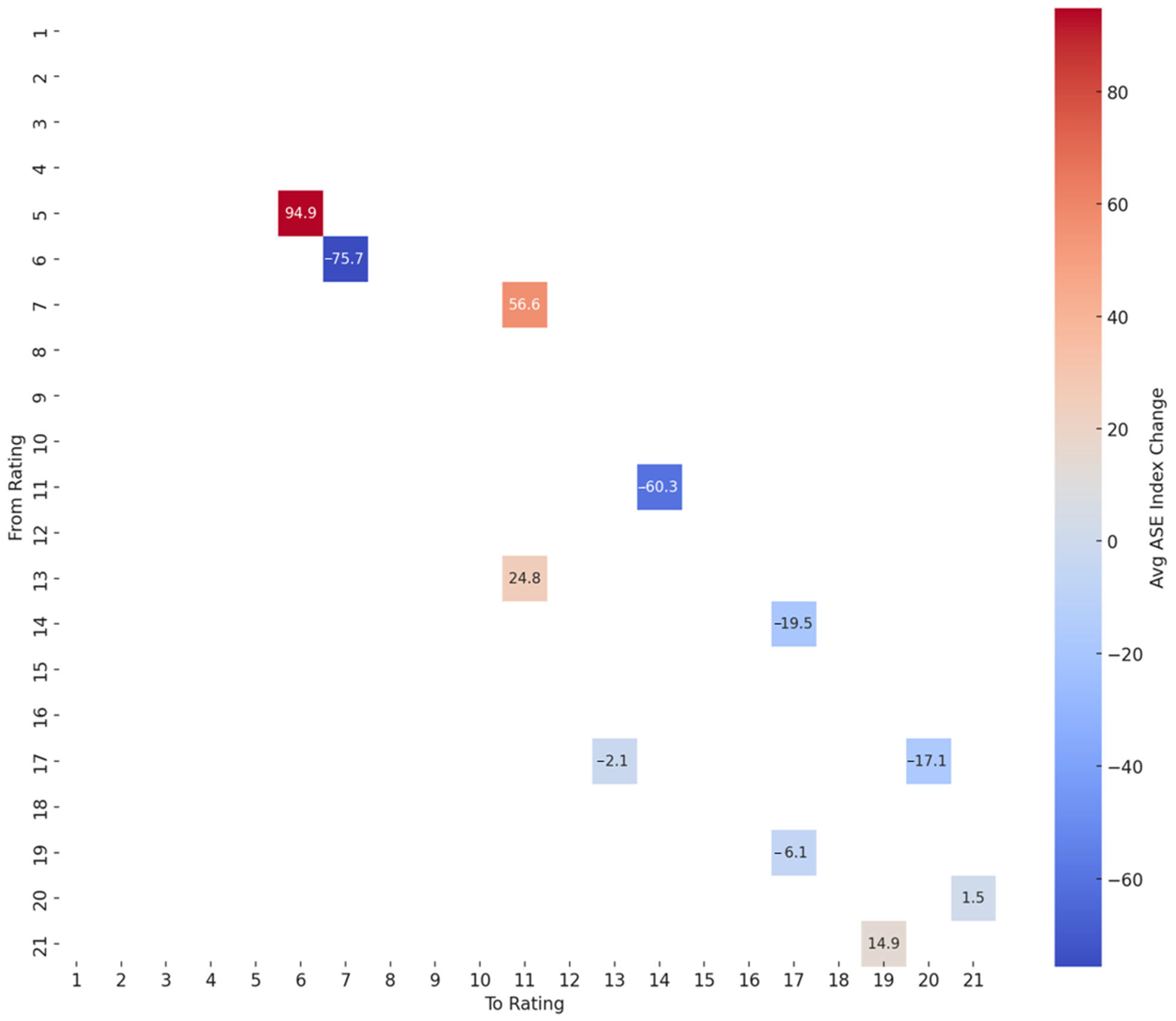
To examine the immediate market response to sovereign credit rating changes, an event study methodology was applied to the ASE Index around major Moody’s rating transitions for Greece between 2004 and 2024. Events were identified as discrete instances where Greece’s credit rating shifted by two or more notches, capturing only the most significant upgrades or downgrades (Appendix A.8). For each event, a symmetric event window of ±5 trading days was constructed, and the ASE Index returns were normalized relative to the event date (t = 0). By aggregating returns across all such events, we computed the average abnormal price movement before and after rating announcements.

The results (Figure 7) revealed that the ASE Index tended to decline slightly in the days leading up to a downgrade and continued to underperform immediately after the event. However, the magnitude of the average market reaction was modest, suggesting that rating changes may have been anticipated or that their informational content was partially absorbed before formal announcements. The absence of sharp corrections post-event also points to a relatively efficient market reaction, where sovereign ratings serve more as confirmatory signals than as surprise shocks. These findings are consistent with the literature [24,25] suggesting limited short-term market impact of credit ratings in countries with relatively transparent fiscal environments.

3.7. Reward Matrix

To quantify the market response to changes in sovereign credit ratings, a reward matrix was constructed by analyzing daily transitions in Greece’s Moody’s credit ratings and the corresponding changes in the ASE Index over the period 2004–2024 (Appendix A.9). The methodology involved identifying all observed transitions between consecutive rating levels (e.g., from Ba2 to Ba3), and for each transition, calculating the change in the ASE Index from the day before to the day of the rating shift. These index changes were then aggregated and averaged to populate a 21 × 21 reward matrix, with rows representing the originating rating and columns representing the target rating. Transitions with insufficient or no observations were left blank to preserve data integrity. The resulting matrix (Figure 8) captures the average market “reward” (or penalty) associated with each rating adjustment. The rows represent the origin ratings (e.g., A1), while the columns correspond to the target ratings (e.g., Ba2). The color intensity and numerical values reflect the magnitude and direction of the market’s response—positive or negative—to each specific rating transition. This matrix constitutes the analytical basis for the optimal path analysis and provides empirical insight into the historical impact of various credit rating events on market performance.

The analysis revealed that downgrades were generally associated with negative average changes in the ASE Index, while upgrades—although less frequent—tended to show modest positive reactions. The matrix is notably sparse, reflecting Moody’s tendency to move ratings gradually and the rarity of abrupt multi-notch transitions. The observed asymmetry in market responses to credit rating changes aligns with findings in the existing literature, which suggests that downgrades tend to exert stronger and more immediate effects on financial markets compared to upgrades [16,23]. This phenomenon is often attributed to the informational asymmetry inherent in negative credit events, which are perceived as signals of increased uncertainty or deteriorating fiscal conditions. The sparsity of the reward matrix reflects Moody’s cautious approach to rating adjustments, consistent with [26], which highlights the agency’s preference for incremental changes over abrupt multi-notch shifts. Such structural sparsity underscores the role of path dependency in sovereign credit risk assessments. By quantifying the average ASE Index responses to individual rating transitions, the reward matrix provides a data-driven foundation for understanding how the equity market historically priced sovereign credit risk, and it served as a critical input for the optimal path analysis of rating recovery or deterioration.

3.8. Optimal Rating Path Optimization

To identify the most advantageous sequences of sovereign credit rating changes from a market perspective, an optimal path analysis was conducted using the reward matrix derived from Moody’s rating transitions and corresponding ASE Index movements. Each cell in the reward matrix represented the average change in the ASE Index associated with a specific transition between two rating levels. This matrix was transformed into a directed graph, where nodes represented credit ratings and edges represented observed transitions weighted by the negative of the reward (i.e., ASE Index gain or loss), enabling the use of shortest-path algorithms to find the route that maximized market value. Using Dijkstra’s algorithm, the analysis computed optimal rating improvement or deterioration paths by minimizing cumulative market cost (or equivalently, maximizing expected gain). For instance, the optimal downgrade path from A1 to Ba1 was found to be A1 → A2 → A3 → Ba1, with a cumulative expected ASE Index gain of +75.76 points (Appendix A.10). Similarly, the optimal upgrade path from C to Ba1 proceeded through a sequence of intermediate speculative ratings and resulted in a total expected gain of +31.50 points (Appendix A.11). To identify historically favorable rating trajectories, an exhaustive optimal path analysis was performed using Greece’s observed sovereign credit rating transitions and corresponding ASE Index responses between 2004 and 2024 (Appendix A.12). The results of all reachable paths are presented in

Table 4. List of all reachable rating transitions (from one rating to another) along with their optimal paths and the expected ASE Index gains (Greece, 2004–2024).

From	To	Path	Expected ASE Index Gain/Loss
A1	A2	A1 → A2	94.87
A1	A3	A1 → A2 → A3	19.2
A1	Ba1	A1 → A2 → A3 → Ba1	75.76
A1	B1	A1 → A2 → A3 → Ba1 → B1	15.41
A1	Ba3	A1 → A2 → A3 → Ba1 → B1 → Caa1 → Ba3	−6.12
A1	Caa1	A1 → A2 → A3 → Ba1 → B1 → Caa1	−4.06
A1	Ca	A1 → A2 → A3 → Ba1 → B1 → Caa1 → Ca	−21.17
A1	Caa3	A1 → A2 → A3 → Ba1 → B1 → Caa1 → Ca → C → Caa3	−4.79
A1	C	A1 → A2 → A3 → Ba1 → B1 → Caa1 → Ca → C	−19.7
A2	A3	A2 → A3	−75.67
A2	Ba1	A2 → A3 → Ba1	−19.11
A2	B1	A2 → A3 → Ba1 → B1	−79.46
A2	Ba3	A2 → A3 → Ba1 → B1 → Caa1 → Ba3	−100.99
A2	Caa1	A2 → A3 → Ba1 → B1 → Caa1	−98.93
A2	Ca	A2 → A3 → Ba1 → B1 → Caa1 → Ca	−116.04
A2	Caa3	A2 → A3 → Ba1 → B1 → Caa1 → Ca → C → Caa3	−99.66
A2	C	A2 → A3 → Ba1 → B1 → Caa1 → Ca → C	−114.57
A3	Ba1	A3 → Ba1	56.56
A3	B1	A3 → Ba1 → B1	−3.79
A3	Ba3	A3 → Ba1 → B1 → Caa1 → Ba3	−25.32
A3	Caa1	A3 → Ba1 → B1 → Caa1	−23.26
A3	Ca	A3 → Ba1 → B1 → Caa1 → Ca	−40.37
A3	Caa3	A3 → Ba1 → B1 → Caa1 → Ca → C → Caa3	−23.99
A3	C	A3 → Ba1 → B1 → Caa1 → Ca → C	−38.9
Ba1	B1	Ba1 → B1	−60.35
Ba1	Ba3	Ba1 → B1 → Caa1 → Ba3	−81.88
Ba1	Caa1	Ba1 → B1 → Caa1	−79.82
Ba1	Ca	Ba1 → B1 → Caa1 → Ca	−96.93
Ba1	Caa3	Ba1 → B1 → Caa1 → Ca → C → Caa3	−80.55
Ba1	C	Ba1 → B1 → Caa1 → Ca → C	−95.46
B1	Ba1	B1 → Caa1 → Ba3 → Ba1	3.24
B1	Ba3	B1 → Caa1 → Ba3	−21.53
B1	Caa1	B1 → Caa1	−19.47
B1	Ca	B1 → Caa1 → Ca	−36.58
B1	Caa3	B1 → Caa1 → Ca → C → Caa3	−20.2
B1	C	B1 → Caa1 → Ca → C	−35.11
Ba3	Ba1	Ba3 → Ba1	24.77
Ba3	B1	Ba3 → Ba1 → B1	−35.58
Ba3	Caa1	Ba3 → Ba1 → B1 → Caa1	−55.05
Ba3	Ca	Ba3 → Ba1 → B1 → Caa1 → Ca	−72.16
Ba3	Caa3	Ba3 → Ba1 → B1 → Caa1 → Ca → C → Caa3	−55.78
Ba3	C	Ba3 → Ba1 → B1 → Caa1 → Ca → C	−70.69
Caa1	Ba1	Caa1 → Ba3 → Ba1	22.71
Caa1	B1	Caa1 → Ba3 → Ba1 → B1	−37.64
Caa1	Ba3	Caa1 → Ba3	−2.06
Caa1	Ca	Caa1 → Ca	−17.11
Caa1	Caa3	Caa1 → Ca → C → Caa3	−0.73
Caa1	C	Caa1 → Ca → C	−15.64
Ca	Ba1	Ca → C → Caa3 → Caa1 → Ba3 → Ba1	32.97
Ca	B1	Ca → C → Caa3 → Caa1 → Ba3 → Ba1 → B1	−27.38
Ca	Ba3	Ca → C → Caa3 → Caa1 → Ba3	8.2
Ca	Caa1	Ca → C → Caa3 → Caa1	10.26
Ca	Caa3	Ca → C → Caa3	16.38
Ca	C	Ca → C	1.47
Caa3	Ba1	Caa3 → Caa1 → Ba3 → Ba1	16.59
Caa3	B1	Caa3 → Caa1 → Ba3 → Ba1 → B1	−43.76
Caa3	Ba3	Caa3 → Caa1 → Ba3	−8.18
Caa3	Caa1	Caa3 → Caa1	−6.12
Caa3	Ca	Caa3 → Caa1 → Ca	−23.23
Caa3	C	Caa3 → Caa1 → Ca → C	−21.76
C	Ba1	C → Caa3 → Caa1 → Ba3 → Ba1	31.5
C	B1	C → Caa3 → Caa1 → Ba3 → Ba1 → B1	−28.85
C	Ba3	C → Caa3 → Caa1 → Ba3	6.73
C	Caa1	C → Caa3 → Caa1	8.79
C	Ca	C → Caa3 → Caa1 → Ca	−8.32
C	Caa3	C → Caa3	14.91

, including the full sequence of transitions and the total expected ASE gain for each path. These results reveal both upgrade and downgrade sequences with positive or negative market implications. The analysis highlights the critical role of path dependency in sovereign credit dynamics, and the optimal paths provide a practical reference for modeling rating-based market reactions or designing rating recovery strategies.

Among the optimal rating trajectories extracted from Greece’s sovereign credit history, notable examples include the downgrade sequence A1 → A2 → A3 → Ba1, which results in a substantial cumulative ASE Index gain of +75.76 points. The unexpected market gains observed along some downgrade trajectories likely reflect anticipatory investor behavior or policy interventions (e.g., EU/IMF support) that mitigated investor panic. This supports the hypothesis that the context and credibility of fiscal policy shape the valuation of credit signals more than the notching itself. Similarly, the upgrade path C → Caa3 → Caa1 → Ba3 → Ba1 yields a positive expected ASE Index gain of +31.50 points, highlighting that recovery transitions—though rare—can restore market confidence over time when accompanied by structural reforms.

These findings align with the conclusions of the relevant literature [24], which show that markets react asymmetrically to downgrades and upgrades, with more severe effects concentrated around the speculative–investment grade threshold. Additionally, ref. [22] emphasized that rating transitions during fiscal crises may carry less new information, particularly when they confirm trends already priced in by the investors. The Greece case reinforces these dynamics, as market reactions to rating shifts often depended not solely on the notching but on the broader economic context and the credibility of corrective measures. Thus, the optimal path analysis does not merely track credit changes but reveals the underlying market psychology that governs sovereign risk pricing.

4. Discussion

Credit rating announcements in Greece exhibit a limited immediate influence on the stock market, suggesting that investors often anticipate these events. This behavior implies a degree of informational efficiency and market maturity, whereby ratings serve more as confirmation than as news. Additionally, sudden downgrades do not appear to trigger significant market destabilization, reinforcing the notion that Greece’s financial ecosystem has evolved greater resilience and transparency since the crisis period. Notably, the analysis highlights that the most impactful market responses arise not from isolated rating shifts, but from sequential downgrade trajectories, underscoring the structural importance of cumulative perceptions in sovereign risk evaluation.

These findings suggest several actionable pathways for policymakers. First, continued emphasis on transparency and predictability in fiscal reporting is crucial, as it enables markets to price in developments prior to formal credit rating changes. Second, advancing investor education initiatives may help market participants better understand the context and limitations of sovereign ratings, particularly in relatively stable economies. Finally, the development of early-warning systems based on reward matrix behavior and optimal downgrade paths could provide preemptive insights for regulatory authorities and institutional investors, enabling more agile and informed responses to emerging fiscal vulnerabilities.

The application of algebraic combinatorics to sovereign credit dynamics not only enhances structural modeling but also aligns with key principles in behavioral finance and decision theory. In particular, the poset and transition graph representations capture how economic agents—such as investors or credit rating agencies—form expectations and update beliefs in response to ordinal information rather than cardinal precision. This resonates with the concept of bounded rationality, where agents rely on discrete heuristics and comparative judgments rather than precise calculations. Furthermore, the observed path-dependency in rating transitions mirrors prospect theory’s emphasis on reference-dependent evaluation: markets tend to react more strongly to deteriorations than to equivalent improvements. The combinatorial models developed in this study—especially the reward matrix and optimal transition paths—formalize such behavioral asymmetries by quantifying investor responses to sequences of credit events. Thus, algebraic structures serve not only as mathematical scaffolds but as conceptual analogues for understanding how cognitive biases and informational frictions shape sovereign risk pricing.

Despite the methodological contributions and empirical insights of this study, limitations should be acknowledged. First, while Moody’s credit ratings are treated as ordinal variables for quantitative analysis, the transformation into an integer scale does not capture the nonlinear nature of credit risk differentials between rating levels. Second, the study focuses exclusively on Greece, which, while offering a unique case of sovereign credit volatility, may limit the generalizability of the findings to other economies with different institutional frameworks or market structures. The focus on Greece from 2004 to 2024 offers a rich and contextually significant case study, given the country’s unique trajectory through the Eurozone debt crisis, multiple credit rating downgrades, and subsequent stabilization efforts. This temporal and geographical specificity allows for a detailed analysis of market responses to rating shocks under conditions of fiscal stress, institutional intervention, and systemic uncertainty. However, the findings inevitably reflect Greece’s idiosyncratic macroeconomic and political environment, which may limit the generalizability of the results. To enhance the empirical contribution, future research could apply the same methodological framework—reward matrix construction, optimal path analysis, and event study techniques—to a broader set of economies. In particular, extending the analysis to other EU periphery countries (e.g., Portugal, Spain, Italy, or Ireland) would allow for comparative insights and the identification of common or divergent patterns in how sovereign rating dynamics affect financial markets. Such cross-country extensions could also help disentangle country-specific effects from broader regional or institutional influences, thereby increasing the robustness and policy relevance of the conclusions. Third, the absence of significant Granger causality between changes in sovereign credit ratings and movements in the Athens Stock Exchange indicates that ratings may function primarily as lagging indicators, formalizing information already priced by investors. While this finding is consistent with the view that rating agencies confirm rather than lead prevailing trends, it could also reflect anticipation effects—investors repositioning before announcements—or endogeneity if market conditions influence rating decisions. Moreover, linear VAR models may miss nonlinear or threshold relationships (e.g., sharp reactions when crossing the speculative-grade boundary). Future research could explore these possibilities using threshold VARs, regime-switching specifications, or instrumental-variable approaches to isolate causal channels more effectively. Fourth, the reward matrix is constructed from historical transitions, and as such, it reflects past market behavior rather than predictive causality. The application of a reward matrix and optimal path modeling through Dijkstra’s algorithm provides valuable insights into the asymmetrical nature of market responses to sovereign credit rating transitions. By treating rating evolution as a path optimization problem, this approach not only captures the disproportionate effects of downgrades but also quantifies the cumulative market impact of sequential rating changes. The framework enables scenario-based exploration of optimal or adverse trajectories, grounded in empirically observed market behavior. However, this method implicitly assumes that market reactions to rating events are stable over time. In reality, significant regime shifts—such as the implementation of bailout programs, entry into fiscal adjustment mechanisms, or changes in monetary policy credibility—may alter investor sensitivity to rating announcements. Consequently, while the model performs well under normal conditions, its applicability may be limited during periods of structural change, suggesting the need for extensions incorporating time-varying reward matrices or regime-switching specifications. Finally, the static structure of the rating transition graph does not account for potential temporal changes in investor behavior or credit rating agency methodologies over the two-decade study period.

Future research may extend this methodology to corporate bond rating dynamics, banking stress test scenarios, or sovereign risk modeling in emerging markets with volatile credit histories.

5. Conclusions

This study provides an in-depth and methodologically integrated investigation into the relationship between sovereign credit rating transitions and domestic equity market performance, with Greece serving as a case study spanning the period 2004–2024. By combining techniques from network theory, econometrics, and financial event analysis, this research advances the understanding of the mechanisms through which credit ratings interact with market dynamics in the context of a fiscally volatile yet institutionally evolving economy. The central finding—that rating announcements exert limited immediate influence on equity markets—challenges the conventional assumption that sovereign credit ratings are primary drivers of investor behavior.

While rolling-window correlation and Granger causality tests reveal no significant or stable predictive power of ratings on the ASE Index, this lack of short-term responsiveness must not be misinterpreted as irrelevance. Rather, the reward matrix and optimal rating path analyses demonstrate that markets respond more meaningfully to rating transitions that unfold in sequences, particularly those indicating sustained deterioration in creditworthiness. These patterns suggest that investors are more sensitive to the trajectory and persistence of sovereign risk signals than to single, abrupt announcements. This insight is critical for understanding how credit risk is interpreted and priced in environments where expectations are formed through multiple channels—including macroeconomic indicators, political developments, and institutional disclosures.

The major focus and contribution of this paper lies in its methodological innovation. It introduces a framework that merges temporal analysis with topological modeling to explore credit rating transitions not only as discrete events but as elements of a broader structural process. The construction of directed graphs, poset representations of rating hierarchies, and the implementation of reward matrices constitute a novel approach to capturing the path-dependent and relational nature of sovereign rating dynamics. This framework departs from traditional linear models and offers a richer interpretive lens, suitable for detecting latent market patterns and long-run interdependencies.

From a scientific quality perspective, the study maintains analytical rigor by grounding each methodological component in both empirical validity and theoretical relevance. The use of daily, real-world data from Moody’s and the Athens Stock Exchange, coupled with the implementation of widely accepted statistical techniques, ensures both robustness and reproducibility. Furthermore, the integration of visual modeling with quantitative analysis allows for a multi-layered understanding that is both interpretable and generalizable, paving the way for applications beyond the Greek case.

Overall, the study concludes that sovereign credit ratings retain symbolic and institutional relevance. Their immediate influence on market behavior—especially in mature or crisis-tempered economies like Greece—appears to be attenuated by the informational efficiency of investors. It is in the structural unfolding of transitions, rather than in isolated rating changes, that meaningful market responses are observed. This finding has important implications for credit rating agencies, policymakers, and investors, suggesting that attention should be directed toward the early detection of sequential downgrade trajectories rather than overreliance on headline rating shifts. As such, the analytical tools and insights developed herein offer valuable contributions to the scientific literature on financial risk, market behavior, and credit assessment.

References

1. Griffith, D.A. Some comments about zero and non-zero eigenvalues from connected undirected planar graph adjacency matrices. AppliedMath 2023, 3, 771–798. [Google Scholar] [CrossRef]
2. Dutta, A.; Kumar, S.; Munjal, D.; Kumar, P.K. The Search-o-Sort Theory. AppliedMath 2025, 5, 64. [Google Scholar] [CrossRef]
3. Cerný, A. Mathematical Techniques in Finance: Tools for Incomplete Markets; Princeton University Press: Princeton, NJ, USA, 2009. [Google Scholar] [CrossRef]
4. Sandfeld, S. Combinatorics and probabilities. In Materials Data Science: Introduction to Data Mining, Machine Learning, and Data-Driven Predictions for Materials Science and Engineering; Springer International Publishing: Cham, Switzerland, 2023; pp. 69–102. [Google Scholar] [CrossRef]
5. Caldarelli, G.; Battiston, S.; Garlaschelli, D.; Catanzaro, M. Emergence of complexity in financial networks. Complex Netw. 2004, 1, 399–423. [Google Scholar] [CrossRef]
6. Battiston, S.; Puliga, M.; Kaushik, R.; Tasca, P.; Caldarelli, G. Debtrank: Too central to fail? Financial networks, the Fed and systemic risk. Sci. Rep. 2012, 2, 541. [Google Scholar] [CrossRef] [PubMed]
7. Hajizadeh, E.; Mahootchi, M. Optimized radial basis function neural network for improving approximate dynamic programming in pricing high dimensional options. Neural Comput. Appl. 2018, 30, 1783–1794. [Google Scholar] [CrossRef]
8. Brandão, L.E.; Dyer, J.S.; Hahn, W.J. Using binomial decision trees to solve real-option valuation problems. Decis. Anal. 2005, 2, 69–88. [Google Scholar] [CrossRef]
9. Li, Y.; Gu, C.; Dullien, T.; Vinyals, O.; Kohli, P. Graph matching networks for learning the similarity of graph structured objects. In Proceedings of the International Conference on Machine Learning, Long Beach, CA, USA, 9–15 June 2019; pp. 3835–3845. Available online: https://proceedings.mlr.press/v97/li19d/li19d.pdf (accessed on 6 June 2025).
10. Lando, D. Credit risk modeling. In Handbook of Financial Time Series; Andersen, T.G., Davis, R.A., Kreiss, J.-P., Mikosch, T., Eds.; Springer: Berlin/Heidelberg, Germany, 2009; pp. 787–798. [Google Scholar] [CrossRef]
11. Xu, J.; Wickramarathne, T.L.; Chawla, N.V. Representing higher-order dependencies in networks. Sci. Adv. 2016, 2, e1600028. [Google Scholar] [CrossRef] [PubMed]
12. Trotter, W.T. Combinatorics and Partially Ordered Sets; Johns Hopkins University Press: Baltimore, MD, USA, 1992. [Google Scholar]
13. Avery, J.E.; Moyen, J.Y.; Růžička, P.; Simonsen, J.G. Chains, antichains, and complements in infinite partition lattices. Algebra Univ. 2018, 79, 37. [Google Scholar] [CrossRef]
14. Yue, L.; Lv, Y. VIKOR optimization decision model based on poset. J. Intell. Fuzzy Syst. 2025, 48, 673–689. [Google Scholar] [CrossRef]
15. White, L.J. The credit rating industry: An industrial organization analysis. In Ratings, Rating Agencies and the Global Financial System; Levich, R.M., Majnoni, G., Reinhart, C.M., Eds.; Springer: Boston, MA, USA, 2002; pp. 41–63. [Google Scholar] [CrossRef]
16. Gonzalez, F.; Haas, F.; Johannes, R.; Persson, M.; Toledo, L.; Violi, R.; Zins, C. Market Dynamics Associated with Credit Ratings—A Literature Review; European Central Bank: Frankfurt, Germany, 2004; Available online: https://www.econstor.eu/bitstream/10419/154469/1/ecbop016.pdf (accessed on 6 June 2025).
17. Alogoskoufis, G. Greece’s Sovereign Debt Crisis: Retrospect and Prospect; LSE Hellenic Observatory: London, UK, 2012; Available online: https://eprints.lse.ac.uk/42848/1/GreeSE%20No54.pdf (accessed on 6 June 2025).
18. Moody’s Investors Service. Sovereign Bond Ratings. Moody’s Ratings Methodology. Available online: https://www.moodys.com/researchdocumentcontentpage.aspx?docid=PBC_151479 (accessed on 6 June 2025).
19. Bratis, T.; Kouretas, G.P.; Laopodis, N.T.; Vlamis, P. Sovereign credit and geopolitical risks during and after the EMU crisis. Int. J. Financ. Econ. 2024, 29, 3692–3712. [Google Scholar] [CrossRef]
20. Lee Rodgers, J.; Nicewander, W.A. Thirteen ways to look at the correlation coefficient. Am. Stat. 1988, 42, 59–66. [Google Scholar] [CrossRef]
21. Kaminsky, G.; Schmukler, S.L. Emerging market instability: Do sovereign ratings affect country risk and stock returns? World Bank Econ. Rev. 2002, 16, 171–195. [Google Scholar] [CrossRef]
22. Afonso, A.; Furceri, D.; Gomes, P. Sovereign credit ratings and financial markets linkages: Application to European data. J. Int. Money Financ. 2012, 31, 606–638. [Google Scholar] [CrossRef]
23. Hill, P.; Faff, R. The market impact of relative agency activity in the sovereign ratings market. J. Bus. Financ. Account. 2010, 37, 1309–1347. [Google Scholar] [CrossRef]
24. Gande, A.; Parsley, D.C. News spillovers in the sovereign debt market. J. Financ. Econ. 2005, 75, 691–734. [Google Scholar] [CrossRef]
25. Ferreira, M.A.; Gama, P.M. Does sovereign debt ratings news spill over to international stock markets? J. Bank. Financ. 2007, 31, 3162–3182. [Google Scholar] [CrossRef]
26. Cantor, R.; Packer, F. Determinants and impact of sovereign credit ratings. Econ. Policy Rev. 1996, 2, 37–53. [Google Scholar] [CrossRef]
Figure 1. An illustrative example of a simplified credit rating transition graph.
Appliedmath 05 00090 g001
Figure 2. A simplified reward matrix heatmap that illustrates how the market may respond to transitions between three hypothetical credit ratings: A (high), B (moderate), and C (low).
Appliedmath 05 00090 g002
Figure 3. A hypothetical example of an optimal rating path, representing the sequence of credit ratings that maximizes cumulative market reward over a given time horizon.
Appliedmath 05 00090 g003
Figure 4. (a) Poset (partially ordered set) representation of Moody’s credit rating hierarchy; (b) Poset (partially ordered set) representation of the Moody’s credit rating hierarchy for Greece (2004–2024). Nodes are vertically ordered by credit quality. Each node represents a rating category (e.g., Aaa, Aa1, …, C). Edges show the strict ordering from higher to lower credit quality.
Appliedmath 05 00090 g004
Figure 5. Moody’s credit rating transition graph for Greece (2004–2024). Nodes represent credit rating categories (e.g., A1, Ba2). Directed edges indicate observed transitions from one rating to another. Edge weights show how frequently each transition occurred.
Appliedmath 05 00090 g005
Figure 6. The rolling 90-day Pearson correlation between Moody’s credit rating (numerically encoded) and the ASE Index. Negative values indicate that as ratings worsen (higher numbers), the ASE Index tends to decline. Positive values suggest the ASE Index may rise even as ratings worsen, indicating possible market decoupling.
Appliedmath 05 00090 g006
Figure 7. The average percentage change in the ASE Index surrounding major credit rating changes by Moody’s (defined as transitions of two or more notches). Day 0 represents the exact date of the rating announcement. The plotted curve captures the temporal pattern of market response, highlighting the behavior of the ASE Index in the days leading up to and following these significant rating events.
Appliedmath 05 00090 g007
Figure 8. Reward matrix heatmap (average change in the ASE Index associated with each observed Moody’s rating transition).
Appliedmath 05 00090 g008