Article

The Search-o-Sort Theory

1
Department of Computer Science and Engineering, Government College of Engineering and Textile Technology, Serampore 712201, Calcutta, India
2
Department of Master of Computer Applications, G.L. Bajaj Institute of Technology and Management, Greater Noida 201308, Uttar Pradesh, India
3
Department of Information Technology, Government College of Engineering and Textile Technology, Serampore 712201, Calcutta, India
*
Author to whom correspondence should be addressed.
AppliedMath 2025, 5(2), 64; https://doi.org/10.3390/appliedmath5020064
Submission received: 18 April 2025 / Revised: 25 May 2025 / Accepted: 27 May 2025 / Published: 29 May 2025
(This article belongs to the Special Issue Algebraic Combinatorics in Data Science and Optimisation)

Abstract

:
In the modern era of informatics, where data are very important, efficient management of data is necessary and critical. Two of the most important data management techniques are searching and data ordering (technically sorting). Traditional sorting algorithms work in quadratic time O x 2 , and in the optimized cases, they take linearithmic time O x · log x , with no existing method surpass this lower bound, given arbitrary data, i.e., ordering a list of cardinality x in O x · log x ϵ ( x ) ϵ ( x ) > 0 . This research proposes Search-o-Sort, which reinterprets sorting in terms of searching, thereby offering a new framework for ordering arbitrary data. The framework is applied to classical search algorithms,–Linear Search, Binary Search (in general, k-ary Search), and extended to more optimized methods such as Interpolation and Jump Search. The analysis suggests theoretical pathways to reduce the computational complexity of sorting algorithms, thus enabling algorithmic development based on the proposed viewpoint.

1. Introduction

In the digital age, exponential growth of data necessitates the need for efficient data management, for which, sorting and searching hold foundational roles in information organization and retrieval. Sorting is fundamental to numerous computational tasks, with widespread applications from database indexing to network routing and machine learning.

1.1. General Context

The objective of Sorting Algorithms is to arrange a collection of elements in a specific order (by their magnitude). If one were to attempt to establish a broad, amorphous explanation, one could begin by saying that it is a procedure that examines the collection of all permutations P ( A ) for a potential permutation in which each of the components that make up the index is monotonically organized. It is guaranteed that there always exists an instance P i P A such that in P i A , A i A i + 1 or A i A i + 1 i n , where n is the cardinality of the dataset. The classical sorting lower bound is well-established through decision tree models, where each comparison narrows the set of possible permutations. This results in a minimum of log 2 ( n ! ) comparisons, which, by Stirling’s approximation, gives rise to the Ω ( n log n ) bound (refer to Appendix A).
Claim. 
For any sorting Algorithm, the minimal time, any Algorithm can hit is Ω n log 2 n .
Proof. 
Let us attempt to understand sorting in the context of searching (which is the backbone of this research). Each categorized component ultimately seeks its correct position within the set. Assume it is required to evacuate the element α i to its original location. To return to its original location, one will have to look in as many n places as possible. Now, after it has been dumped at its original location and moved on to the subsequent element of α i , to evict it to its true location, one must look for it at most n 1 locations, and the number of locations to be sought varies as follows: n 3 , n 4 , n 5 , n 6 , …, 1. There are numerous searching algorithms available, such as linear search, binary search, and interpolation search [1], but the quickest searching technique created thus far without enforcing any stringent restrictions is binary search [2], which conducts searches in logarithmic time T search optimal ( x ) = log 2 x , for a list of cardinality x . So, the total time, as per the computational complexities, will be
T n = log 2 n + log 2 n 1 + log 2 n 2 + + log 2 1
which can be further delineated as
T n = log 2 i = 0 n 1 n i = log 2 n !
Now, there exist some approximations with bounds for the general factorial, Stirling’s Approximation, and Ramanujan’s Approximation for the Gamma Function, to name a few. In some recent works, it was proved using the aforementioned approximation that the minimum computational time taken by a sorting Algorithm to sort a given set of data is of the order of n log ( n ) without tampering with the general architecture of the processor. Drawing from that work and utilizing Srinivasa Ramanujan’s approximation of the Euler Gamma Function, we can conclude
T ( n ) min = log 2 n !
Thus, from Equation (1), one gets
T ( n ) min n log 2 n
since, Γ 1 + x π x e x 8 x 3 + 4 x 2 + x + θ x 30 6 , where, θ x 1 as x , 3 10 < θ x < 1
   □

1.2. Motivation

Now, since there exists a tight minimal bound for the sorting algorithms, “what’s the point behind this work?” In the reference drawn above, binary searching Algorithm was enforced to search the individual elements before sorting. Over time, scientists and algorithmists came up with a variety of new algorithms that could search for a given key in a hump of data quite optimally (compared to the primitive algorithms). By using these searches, we could make use of some optimized algorithms, which would have an edge over other prevalent algorithms (in terms of sorting).

1.3. Literature Review

In the literature, there exist limited but foundational works on deterministic searching algorithms. These search algorithms serve as the basis for Search-o-Sort. Manna and Waldinger, in their seminal work, “The origin of a binary-search paradigm” [2], introduced 2-ary Search (commonly known as binary search). In recent times, several variants of the binary search exists [3,4,5], operating in O * x log 2 x time (amortized). The proposition of “original” binary search was further extended to 3-ary (ternary) Search [6] by Bajwa et al., and was generalized to k-ary Search [7] by Dutta et al. Contrary to these methods, Interpolation Search [1] suggested a newer perspective for search algorithms. The computational complexity of Interpolation Search is unlike k-ary Search algorithms, which was explained by the authors of Interpolation Search in their follow-up work, “Understanding the complexity of Interpolation Search” [8]. Another out-of-the-box searching Algorithm, Jump Search, was proposed by Shneiderman [9]. These algorithms (in general) serve as the basis for analysis of the proposed Search-o-Sort theory.

1.4. Contribution and Scope

This research introduces Search-o-Sort theory, a conceptual framework that identifies sorting as a composition of iterative searching operations. Thus, in the proposed mathematical formulation, the total cost of sorting Algorithm is modeled as a summation of successive search costs. This model is applied and validated across multiple searching paradigms, Binary Search (in general, k-ary Search), Interpolation Search, and Jump Search. By embedding these search algorithms into the sorting process, we derive computational costs and interpret their implications on the sorting bounds. Our analysis suggests that alternative searching techniques can offer promising directions for reducing effective sorting time, particularly when specialized assumptions or approximations are permitted (which is possible nowadays due to recent advancement in computer architecture).

1.5. Document Structure

The rest of the manuscript is organized as follows, Section 2 introduces the Search-o-Sort theory and its foundational proposition. Section 2.3, Section 2.4, Section 2.5 and Section 2.6 explore the applications of Search-o-Sort theory across k-ary Search, Interpolation Search, and Jump Search, respectively. Finally, Section 3 concludes the paper with insights on the implications of Search-o-Sort theory and scope for future research.

2. Search-o-Sort

One can verify Sorting in the context of Searching, as indicated in the introduction. To summarize, every component that is being ordered is subsequently looking for its correct location in the set. Assume it is required to evacuate the element α i to its original location. To get back to its unique location, one will have to look in all of the n places. Now, once it is dropped at its original place, it will move to the next element of α i , and to evacuate it to its actual place, one will have to search at most n 1 places and in this way, the number of places to be searched varies, coagulated with subsequent decrements. Now, here comes the million-dollar question—which Algorithm should be tested for searching the elemental position invoked with sorting? Works have been published which make use of Binary Search (Equation (2)). Here, firstly, the Search-o-Sort (see Section 2.1) is proposed, and its further expansion for the theoretical provenance is achieved by its application on k-ary (see Section 2.3), Interpolation (see Section 2.4), and Jump Search (see Section 2.6) as intermediate Searching Algorithms for their respective sorting paradigms, as discussed in the Search-o-Sort.

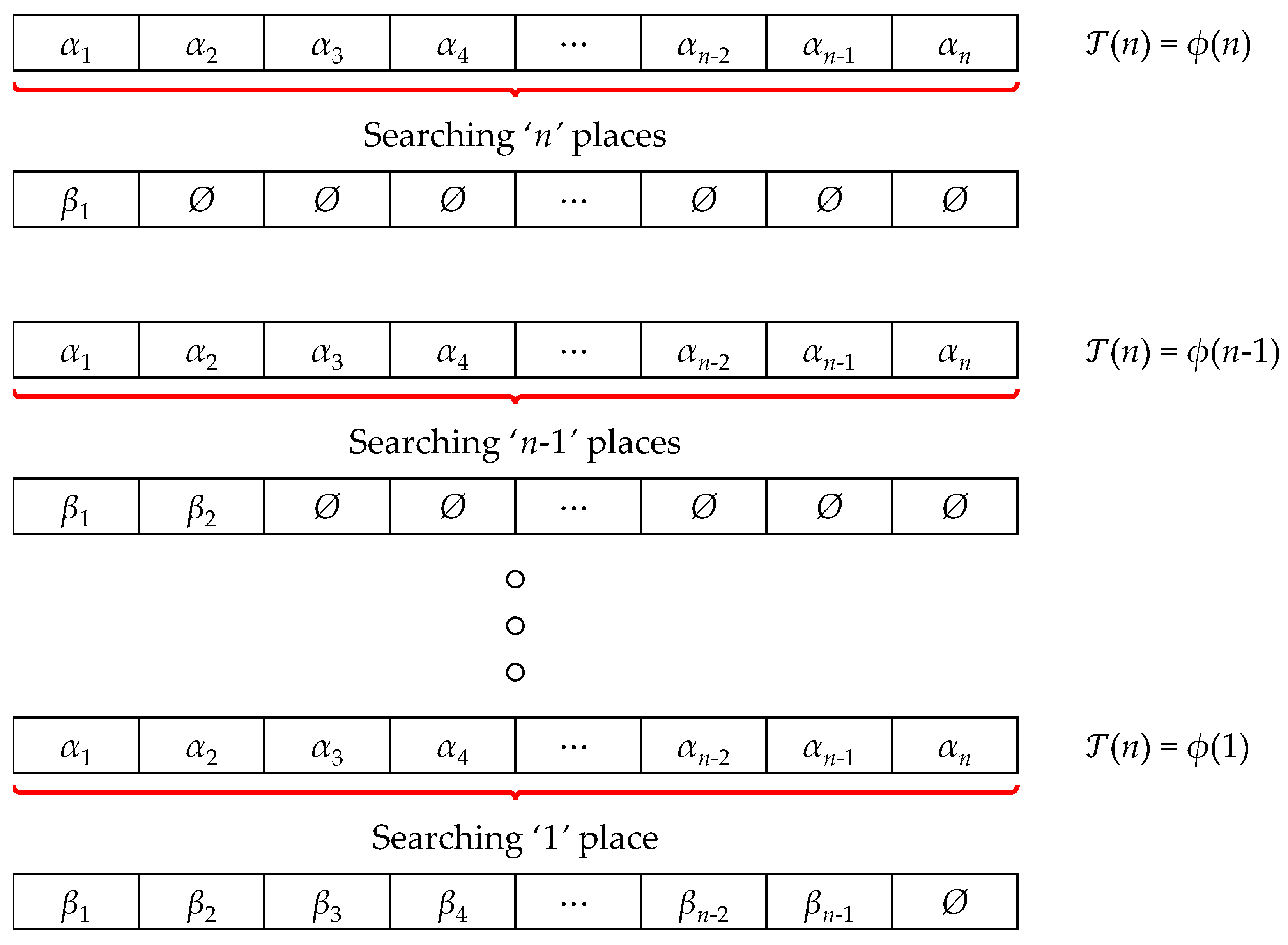
2.1. The Proposition

Suppose we have a set of n elements, α 1 , α 2 , , α n , and we are aiming to find a permutation of this set of n numbers, such that the elements in the permutation follow a monotonic order by their magnitude. Suppose the new permutation after sorting is β 1 , β 2 , , β n . Now, each of these elements β 1 , β 2 , , β n , are selected from the list, α 1 , α 2 , , α n in iterations. The selection cost will depend on the cardinality of the input sequence. Let us suppose, that the cost is ϕ ( n ) . Now, once one selection is complete from the sequence of n entries, it will be left with n 1 more entries to be selected. In the next iteration, the cost would be reduced to ϕ ( n 1 ) , and in the consecutive iterations, the cost will finally converge at ϕ ( 1 ) . Thus, it would be correct to undertake a summation of each of these costs, ϕ ( n ) , ϕ ( n 1 ) , , ϕ ( 1 ) (see Figure 1) to determine the cost of finding the required permutation with elements arranged in monotonic order by their magnitude. So, the Computational Time Complexity of the Sorting Algorithm, which incorporates a Searching Algorithm of Computational Expense, ϕ ( n ) , would be
T sort n = i = 1 n T search i = i = 1 n ϕ i
Corollary 1.
For any sorting Algorithm, if the intermediate searching Algorithm claims a computational expense of ϕ ( n ) , the computational complexity of the sorting Algorithm will be n × ϕ ( n ) .
Proof. 
The proof follows from the proposition (Equation (3)), of the Search-o-Sort, and since it is known that
1 ϕ n i = 1 n + 1 ϕ i d i = O ( n )
NOTE: This proof (and following predicates in the manuscript) intentionally adoptions continuous summation (integrals, over discrete summation) for better convergence (as permissible in an asymptotic setting).
O ( . ) is the Big-Oh Asymptotic Notation (refer to Appendix A.1), and as per the properties of Asymptotes, if one has a function f ( n ) , and if,
g n = O ( f ( n ) )
then,
c · f ( n ) g n ; assuming f ( n ) 0 , g ( n ) 0
Thus c , n 0 ( n > n 0 ) , such that
T sort n = n × T search n
   □
In the following subsections, proposals of the novel sorting paradigms making use of the Interpolation, Jump, and k-ary Searching Techniques as the intermediate are made, and investigated. The aforementioned corollary (Equation (4)) is also verified.

2.2. The Realization

This Search-o-Sort theory might appear circular at first glance, as it invokes binary search as an intermediate for sorting, but this is not the case. This section aims to bridge the realization of the proposed Search-o-Sort theory. To this end, let us consider an infinitely long incline as depicted in Figure 2, and for each integer, there exist respective holes on the hypotenuse. Now, the list to be sorted consists of a fixed set of integers, which are to be sorted by their magnitude. Consider each of the integers as spheres of the respective radius, and the polarity, for example, the integer +7, would fit inside the hole of a radius of 7 units, and positive polarity, i.e., if the ball passes by the −7 hole, it would be repelled by the positive polarity of the hole, and even if it falls inside holes of smaller radius, it would be thrown off by its inertial force (refer Figure 2b. It will only fit inside a hole if both the polarity and the radius match (refer Figure 2c). We would roll each ball corresponding to each integer from the list to be ordered from the hole, and let them roll until they find their exact position.
Now since checking each hole will consume time, we would initially, run the Min-Max Algorithm (refer to Appendix B) in O n to obtain knowledge about the maximum and minimum of the integral list (i.e., assuming inputs to be linearly distributed) to be sorted, and since max min , or max min = O n , we will now start rolling from a smaller index, until the higher index is reached. Now, unrestrictive rolling can be thought of like a linear search, where the ball checks for each hole one by one in a sequential manner. The same unrestricted rolling can be replaced by binary search, wherein the middle hole of the max and min is considered initially, and based on the suitability of the hole, i.e., whether the radius of the hole is greater than or less than that of the ball, the next hole is calculated. This is repeated for all the balls, representing all the entries of the list to be sorted, and thus Sorting is visualized as repeated Sorting.

2.3. k-Ary Sort

In k-ary Search, the list of data is divided into k parts and searched further by comparing elements such as the key, which is the target value subjected to supervision; that is, the element to be found concerning the middle elements of the list. If it is not found, one moves to Boolean-involving inequalities that quantitatively define the estimated position of the element to be searched. This can be considered as the general case of the family to which Binary search (2-ary search) and other searching algorithms like Ternary Search (3-ary search) belong. k-ary Search, being the generic member of all the possible k 1 partition search, contains characteristics that are improvised as an intersection of the characteristics of all the members of the family. In this generic search, the chunk of data is divided into k equal (probably) parts, with potent, k 1 indices that serve as middle points or points of supervision for the search. The generalized equation of one such point of supervision, relating to the initial diametric is
Mid Index λ = + λ × k
where,
, lower bound , upper bound
It works on the principle of Divide and Conquer, where the whole chunk is divided into smaller sub-parts, and solved further. Algorithm 1 shows the Pseudocode for the k-ary Search Algorithm.
Algorithm 1 Pseudocode for the k-ary Search
Require: 
L n L i = i’th entry in the list, and the key, KEY
Ensure: 
i L i = KEY or 1 if not found
  1:
function k-ary Search( L n , k , , , KEY )
  2:
    if   then                        ▹Search space is valid if upper bound ≥ lower bound
  3:
        Initialize a dynamic array M to store the mid indices of partitions
  4:
        for  i = 1 to k 1  do                           ▹Compute k 1 mid points for the interval
  5:
            M + i × k
  6:
        end for
  7:
        for  i = 0 to | M | 1  do               ▹Check if KEY matches any of the mid elements
  8:
           if  L M i = KEY  then
  9:
               return  M i                                                   ▹Return the index if match found
10:
           end if
11:
        end for
12:
        for  i = 0 to | M | 1  do               ▹Search left partition if mid is greater than KEY
13:
           if  L M i > KEY  then
14:
               return k-ary Search( L n , k , , M i 1 , KEY )
15:
           end if
16:
        end for
17:
        for  i = 0 to | M | 1  do                  ▹Search right partition if mid is less than KEY
18:
           if  L M i < KEY  then
19:
               return k-ary Search( L n , k , M i + 1 , , KEY )
20:
           end if
21:
        end for
22:
    end if
23:
    return −1                                        ▹If search interval is invalid or KEY not found
24:
end function
Now, some of the important metrics regarding this k-ary Search Algorithm are as follows:
  • The worst-case time complexity of the k-ary searching algorithm will be T n = k 1 × log k n + O k , which occurs if the target element is present in the indices involving bounds; that is, the starting and the ending indices.
  • The best-case time complexity is T n = Ω ( 1 ) , which occurs if the target element is present at any of the mid indices.
  • The average-case time complexity is T n = Θ ( log k n )
If the key is present somewhere in the list, mathematically,
γ total = 1 × γ 1 + 2 × γ 2 + 3 × γ 3 + 4 × γ 4 + + log k n × γ log k n = i = 1 log k n i × γ i
where, γ k indicates a number of elements that require a total of k comparisons, which is equal to k k 1 Now,
γ total = 1 × γ 1 + 2 × γ 2 + 3 × γ 3 + 4 × γ 4 + + log k n × γ log k n γ total = k log k n × log k n 1 + 1
Now,
γ average = k log k n × log k n 1 + 1 n + 1 = n × log k n 1 + 1 n + 1
So,
T n average = Θ n × log k n 1 + 1 n + 1 Θ log k n
If sorting was sought in terms of the generic k-ary Search, time, as per the computational complexities, will be
T n = log k n + log k n 1 + log k n 2 + + log k 1
which can be further delineated as
T n = log k i = 0 n 1 n i = log k n !
Now, as mentioned earlier, there exist numerous approximations for this general factorial. Here, by making use of the “Very Accurate Approximations for the Factorial Function” by Necdet Batir [10], the result is sought. According to Batir,
n ! 2 π 2 n n e n n + 1 6 + 1 72 n 31 6480 n 2 139 155520 n 3 + 9871 6531840 n 4
Making use of the approximation from Equation (5),
T ( n ) = log k 2 π 2 n n e n + log k n + 1 6 + 1 72 n 31 6480 n 2 139 155520 n 3 + 9871 6531840 n 4 2
which, on asymptotic notations, can be represented as in the order of n log k n
This follows the Search-o-Sort, as T k-ary-search   n T k-ary-sort   n = 1 n .

2.4. Interpolation Sort

Interpolation Search is one of the extrapolations of the Binary Search. It is like searching for a page in a book, where each page is marked distinctly. Algorithm 2 shows the Pseudocode for the Interpolation Search Algorithm.
Now, some of the important metrics regarding this Interpolation Search Algorithm are as follows:
  • The worst-case time complexity of the Interpolation Searching Algorithm will be T n = O n , which occurs if the target element is present in the indices involving bounds; that is, the starting and the ending indices.
  • The Best-Case Time Complexity is T n = Ω ( 1 ) , which occurs if the target element is present at any of the mid indices.
  • In the average case, both cases are considered.
    (a)
    If the key is present in the list.
    (b)
    If it is not present in the list.
If the key is present somewhere in the list, it is assumed that the current search space is from 0 to n + 1 , and n keys are independently drawn from a uniform distribution. As all the elements in the data cluster are independent of each other, it is expected that the expected number of probes γ is bound by a constant. So, the probability that at least one of them is equal to the φ will be
ξ = φ L [ 0 ] L [ n + 1 ] L [ 0 ]
The probability that exactly ψ of them is equal to φ will be
ξ = n ψ ξ ψ ( 1 ξ ) n ψ
So, the number of keys expected to be less than or equal to φ will be
ψ = 1 n ξ = ψ = 1 n n ψ ξ ψ ( 1 ξ ) n ψ = ξ × n
and variance of the following distribution will be
σ 2 = ψ = 1 n ψ ξ × n n ψ ξ ψ ( 1 ξ ) n ψ = ξ × 1 ξ × n
Since, 0 < ξ < 1 , so, ξ × 1 ξ 1 4 and ξ × 1 ξ × n n 4
γ = i 1 i × ξ r Exactly i probes are used = i 1 ξ r Atleast i probes are used
Using bounding conditions of Chebyshev’s Inequality [11],
γ 2 + i 3 1 4 × 1 i 2 2 = 2 + π 2 24 2.42
Let T ( n ) be the average number of probes needed to find a key in an array of size n. Let C be the expected number of probes needed to reduce the search space of size x to x .
T n = C + T ( n )
where C is the bound of the number of probes, C.
T ( n ) Θ log 2 log 2 n
If sorting is sought in terms of the Interpolation Search, time, as per the computational complexities, it will be
T ( n ) = log 2 log 2 n + log 2 log 2 n 1 + log 2 log 2 n 2 + + log 2 log 2 1
which can be further delineated as
T ( n ) = log 2 i = 0 n 1 log 2 n i
Since log 2 ( 1 ) , present at the rear end, will make the argument i = 0 n 1 log 2 n i as zero, and log 2 0 is undefined. Now, in practice, when it comes to searches in data having a single element, it will take a negligible amount of time, say ε , such that ε 0 . In fact, it can be shown that log β x log β x + 1 0 as x 1 and log β x log β x + 1 1 as x for any base, β . So, its very evident from the observations that 0 log β x log β x + 1 1 x 1 , x R + . To normalize this, the Arithmetic Mean of the range is considered, and due to this assumption, it could be proclaimed that log β x 1 log β x = 1 2 . Finally, i = 0 n 1 log 2 n i could be reformatted as
i = 0 n 1 log 2 n i i = 0 n 1 log 2 n 2 i log 2 n n × 2 i = 0 n 1 i
Coming back to Sorting,
T ( n ) = log 2 ( log 2 n n × 2 i = 0 n 1 i )
which can be further delineated as
T ( n ) = n log 2 log 2 n n 2
A tighter bound to this method could be evicted by making use of the Incomplete Gamma Function. To recall, for Interpolation Search,
T ( n ) = i = 1 n log 2 log 2 ( i )
Now,
log 2 log 2 ( k ) k k + 1 log 2 log 2 ( i ) d i log 2 log 2 ( k + 1 )
k = 1 n log 2 log 2 ( k ) k = 1 n k k + 1 log 2 log 2 ( i ) d i k = 1 n log 2 log 2 ( k + 1 )
In practice, log 2 log 2 ( k ) , for k = 1 will be undefined as log 2 ( 1 ) = 0 mathematically, but in real-life instances of computation, lim k 1 log 2 ( k ) = ε ε 0 .
log 2 ε + k = 2 n log 2 log 2 ( k ) k = 1 n k k + 1 log 2 log 2 ( i ) d i k = 1 n l o g 2 l o g 2 ( k + 1 )
k = 2 n log 2 log 2 ( k ) k = 1 n k k + 1 log 2 log 2 ( i ) d i log 2 ε
k = 2 n log 2 log 2 ( k ) 1 n + 1 log 2 log 2 ( x ) d x log 2 ε
T ( n ) n + 1 log 2 log 2 ( n + 1 ) + Γ 0 , log 2 n + 1 Γ 0 , ε 2 log 2 ε
where
Γ ( 0 , x ) e x x + 1 1 + 1 x + 2 1 + 2 x + 3 1 + 3 = π c
Algorithm 2 Pseudocode for the Interpolation Search
Require: 
L n L i = i’th entry in the list, and the key, KEY
Ensure: 
i L i = KEY or 1 if not found
  1:
function Interpolation Search( L n , KEY )
  2:
     0                                           ▹Initialize the lower bound of the search interval
  3:
     | L n | 1                                      ▹Initialize upper bound of the search interval
  4:
    while  KEY not found do                         ▹Continue searching while KEY not found
  5:
        if  <  then                                      ▹Search interval is invalid; terminate loop
  6:
           break
  7:
        end if
  8:
         M = + ( KEY L ) × L L                                                ▹Linear Interpolation
  9:
        if  L M = KEY  then                                               ▹Return the index if match found
10:
           return  M
11:
        end if
12:
        if  L M > KEY  then                                                     ▹KEY lies in the left partition
13:
            = M 1
14:
        end if
15:
        if  L M < KEY  then                                                  ▹KEY lies in the right partition
16:
            = M + 1
17:
        end if
18:
    end while
19:
    return −1                                      ▹If search interval is invalid or KEY not found
20:
end function
Lemma 1.
π c is related to the bounds of the Exponential Integral, Ei ( x ) = t = x e t t d t as
1 3 x 4 x e t t d t γ + ln x 1 3 x 4 + 11 x 2 36
where,
γ = lim n k = 1 n 1 k ln n
which is the Euler–Mascheroni constant.
Making use of Lemma 1,
1 + 3 x 4 + γ + ln x i π > π c > 1 + 3 x 4 + 11 x 2 36 + γ + ln x i π
where, i = 1 .
So,
π c max = 1 + 3 x 4 + γ + ln x i π
Now,
Γ 0 , log 2 n + 1 = e log 2 n + 1 log 2 n + 1 + 1 1 + 1 log 2 n + 1 + 2 1 + 2 log 2 n + 1 + 3
and
Γ 0 , ε = e ε ε + 1 1 + 1 ε + 2 1 + 2 ε + 3
So, the maximum value of
e log 2 n + 1 log 2 n + 1 + 1 1 + 1 log 2 n + 1 + 2 1 + 2 log 2 n + 1 + 3
will be
1 + 3 log 2 n + 1 4 + γ + ln log 2 n + 1 i π
and that of
max e ε ε + 1 1 + 1 ε + 2 1 + 2 ε + 3 = 1 + 3 ε 4 + γ + ln ε i π
So, from Equation (7),
k = 2 n log 2 log 2 ( k ) = O n + 1 log 2 log 2 ( n + 1 ) = O n log 2 log 2 ( n )
This follows the Search-o-Sort, as T interpolation - search n T interpolation - sort n = 1 n .
NOTE: A general interpolation paradigm is M = + ( KEY L ) p ( L L ) p · ( ) . As per the seminal work by Gonnet et al. [1]; they considered p = 1 (linear interpolation). p > 1 skews the probe towards the upper index, while 0 < p < 1 skews the probe towards the lower index. This does not affect the computational complexity (asymptotically) of Interpolation Search (non-linear), and thus the Search-o-Sort theory holds.

2.5. Extrapolation Sort

In the literature, there are no algorithmic developments that (explicitly) relate to Extrapolation Searching, but for evaluation of the proposed Search-o-Sort Algorithm, a logical development is made in Algorithm 3. It searches for the key beyond the learned range of the sorted dataset by extrapolating the (likely) position of the target.
Now, some of the important metrics regarding Extrapolation Search Algorithm are as follows:
  • The worst-case time complexity of the Extrapolation Searching Algorithm will be T ( n ) = O ( n ) , which occurs if the data are highly skewed, or the extrapolated estimate repeatedly fails to converge toward the target, thus degrading to a sequential or linear-like search.
  • The best-case time complexity is T ( n ) = Ω ( 1 ) , which occurs if the target element lies near the extrapolated index on the first estimation and is found without any iterative refinement.
  • In the average case, both conditions are considered:
    (a)
    If the key is present in the list.
    (b)
    If it is not present in the list.
Algorithm 3 Pseudocode for the Extrapolation Search
Require: 
L n L i = i’th entry in the list, and the key, KEY
Ensure: 
i L i = KEY or 1 if not found
  1:
function Extrapolation Search( L n , KEY )
  2:
     0                                                ▹Initialize lower bound of the search interval
  3:
     | L n | 1                                    ▹Initialize upper bound of the search interval
  4:
    if  L = L  then                                              ▹Check if all elements are the same
  5:
        if  L = KEY  then                                               ▹Return index if the KEY matches
  6:
           return 
  7:
        else
  8:
           return −1                                                     ▹KEY not found in constant array
  9:
        end if
10:
    end if
11:
     M + ( KEY L ) × L L                                   ▹Initial (extrapolated) guess
12:
    if  M < or M >  then            ▹Check for extrapolated index out of bounds
13:
        return −1                                                ▹Extrapolated outside valid interval
14:
    end if
15:
    while  KEY not found do                                   ▹Repeat search until KEY is found
16:
        if  <  then        return −1                    ▹Search interval is invalid; exit loop
17:
           break
18:
        end if
19:
         M + ( KEY L ) × L L                           ▹Recompute extrapolated index
20:
        if  M < or M >  then              ▹Check bounds for new extrapolated index
21:
           return −1                                                ▹Extrapolated outside valid interval
22:
        end if
23:
        if  L M = KEY  then                                                            ▹Return if KEY matches
24:
           return  M
25:
        else if  L M > KEY  then                                    ▹Narrow search to left partition
26:
            M 1
27:
        else                                                               ▹Narrow search to right partition
28:
            M + 1
29:
        end if
30:
    end while
31:
    return −1                                       ▹If search interval is invalid or KEY not found
32:
end function
If the key is present somewhere in the list, it is assumed that the search space is uniformly distributed over [ 0 , n + 1 ] , and n keys are independently drawn from a linear distribution. The goal is to predict the index outside the bounds where the value might lie using extrapolation rather than interpolation. The Apropos Interpolation Search, T ( n ) Θ log 2 log 2 n is obtained by further calculations (similar to its predecessor). Therefore, this follows the Search-o-Sort, as T extrapolation - search n T extrapolation - sort n = 1 n .

2.6. Jump Sort

Jump Search is a searching technique [9] that is well defined for sets with the existence of some sort of order prevailing between them. Its course of action is quite simple, and involves checking for every element in the list L k α , for all k N , with α as the evicted block size, until and unless the match is found, larger than the key of supervision. To find the exact position of the key of supervision in the list, a 1-ary search is performed on the sublist, L k 1 α : L α . The block size to be evicted should be of appropriate optimality. Accordingly, n 2 is one such point, with n being the cardinality of the List L . Algorithm 4 shows the Pseudocode for the Jump Search Algorithm.
Algorithm 4 Pseudocode for the Jump Search
Require: 
L n L i = i’th entry in the list, and the key, KEY
Ensure: 
i L i = KEY or 1 if not found
  1:
function Jump Search( L n , KEY )
  2:
     a 0                                                                                                                     ▹Initialize start of block
  3:
     b n                                                                                                                ▹Initialize end of block
  4:
    while  L min ( b , n ) 1 < KEY  do                                       ▹Jump forward while block’s end is less than KEY
  5:
         a b                                                                                          ▹Move start to end of previous block
  6:
         b b + n                                                                                                   ▹Move end to next block
  7:
        if  a n  then                                                              ▹If start exceeds array bounds, KEY not found
  8:
           return −1
  9:
        end if
10:
    end while
11:
    while  L a < KEY  do                                                             ▹Linear search within the identified block
12:
         a a + 1
13:
        if  a = min ( b , n )  then                                               ▹If end of block reached without finding KEY
14:
           return −1                                                                                                                    ▹ KEY not found
15:
        end if
16:
    end while
17:
    if  L a = KEY  then                                                                                                   ▹KEY found at index a
18:
        return a
19:
    else
20:
        return −1                                                                                                                       ▹ KEY not found
21:
    end if
22:
end function
Now, some of the important metrics regarding this Jump Search Algorithm are as follows:
  • In the worst-case scenario, one has to complete n m jumps (n being the cardinality, m being the size of the block to be evicted) and if the last checked value is greater than the element to be searched for, it performs m 1 comparisons more for a linear search. Hence, on the whole, the number of comparisons in the worst case will be n m + m 1 . So, the worst-case complexity will be O ( n 2 ) .
  • The best-case complexity can be obtained simply from the number of comparisons that need to be performed for supervision, η = n m + m 1 . Now, d η d m = n m 2 + 1 . d η d m will be minimum when m = n . With that being said, the best-case complexity becomes Ω ( 1 ) .
  • The average-case complexity for this Searching Technique is abruptly equal to the worst-case complexity, Θ ( n 2 ) .
If sorting was sought in terms of Jump Search, the time, as per the computational complexities, will be
T n = n + n 1 + n 2 + n 3 + + 1
Before, moving further, let us consider the following corroboration [12]
Claim. 
φ ( x ) × ϕ ( x ) d μ φ ζ ( x ) d μ ζ × ϕ ς ( x ) d μ ς φ x R + & ϕ ( x ) R +
Proof. 
Now, firstly, let us consider a probability distribution, P , and function ψ ( x ) , which is P -measurable. Now, according to Jensen’s Inequality [13],
ψ ( x ) d x ψ ζ ( x ) d x 1 ζ
Now, let us consider the measure, μ , such that the density of the probability distribution, P , concerns the measure ϕ ς ( x ) .
δ P = ϕ ( x ) ϕ ς ( x ) d μ δ μ
Let us consider ψ ( x ) = φ ( x ) × ϕ 1 ς ( x ) , and since 1 ζ + 1 ς = 1
φ ( x ) × ϕ ( x ) d μ = ϕ ς ( x ) d μ φ ( x ) × ϕ 1 ς ( x ) ϕ ( x ) ϕ ς ( x ) d μ d μ
Further,
φ ( x ) × ϕ ( x ) d μ ϕ ς ( x ) d μ φ ζ ( x ) × ϕ ζ × 1 ς ( x ) ϕ ( x ) ϕ ς ( x ) d μ d μ ζ
Finally, it can be concluded that
φ ( x ) × ϕ ( x ) d μ φ ζ ( x ) d μ ζ × ϕ ς ( x ) d μ ς
   □
It is known that 1 n d x x = log x n 1
By making use of the inequality, φ ( x ) × ϕ ( x ) d μ φ ζ ( x ) d μ ζ × ϕ ς ( x ) d μ ς , it can be said,
1 n d x x = 1 × 1 x d x x = 1 n d x 2 × x = 1 n 1 x 2 d x 2 = n 2 1 n 2
which can be reformatted as log n n 2 1 n 2 . Now, for high values of n, or in just terms, when, n , log n n 2 will give us a good bound.
Now, coming back to Sorting,
T ( n ) = i = 0 n 1 n i 2 = i = 0 n 1 log n i = log i = 0 n 1 n i
which can be further delineated on asymptotic notations, and can be represented as in the order of n log n or n n , (Equation (9)) to stay in accordance with the assumption mentioned above.
This follows the Search-o-Sort Theory, as T jump - search n T jump - sort n = 1 n .

3. Conclusions

This Search-o-Sort theory is a bridge between Sorting and Searching Algorithms which seeks to merge the notions constructively. In the previous works, the minimum time T ( n ) that could be achieved was sought to be n log 2 n , which was attainable by making use of Binary Search. Now, in this research, its domain is extended to a more generic one. Sorting enhanced with k-ary search, which gave a minimal worst-case time complexity of n log k n is introduced. Further, we made use of the Interpolation Search, which indeed comes with some requisites, but still, assuming that the ample requirements being provided, it managed to fetch a computational time of the order n log 2 log 2 n n 2 . Further, the method was improvised with the notions of Incomplete Gamma Function, or digamma function, to obtain a Computational Advanced Complexity, in terms of the Big—Oh asymptotic as, O n log 2 log 2 ( n ) . Lastly, we made use of Jump Search, which comes with a computational complexity of the order n , which when implemented in Sorting, gave a computational complexity of i = 0 n 1 x = 1 x = n i d x x . Some scopes of further research that could be considered are as follows:
  • A tighter bound, if possible, could be searched for log 2 i = 0 n 1 log 2 n i .
  • An even tighter bound, if possible, could be searched for i = 0 n 1 n i 2 .
Figure 3 draws a comparative graphical study of the algorithms that are emphasized as a primary part of the research.

Author Contributions

Conceptualization, A.D. and S.K.; Methodology, A.D.; Software, P.K.K.; Validation, S.K., D.M. and P.K.K.; Formal Analysis, D.M.; Investigation, P.K.K.; Resources, D.M.; Data Curation, A.D.; Writing—Original Draft Preparation, A.D.; Writing—Review and Editing, P.K.K.; Visualization, S.K.; Supervision, P.K.K.; Project Administration, S.K. All authors have read and agreed to the published version of the manuscript.

Funding

This research received no external funding.

Data Availability Statement

The original contributions presented in this study are included in the article material. Further inquiries can be directed to the corresponding author.

Conflicts of Interest

The authors declare no conflicts of interest.

Appendix A. Asymptotic Notations

Asymptotic notation is a mathematical tool that is used to understand growth of any function, particularly in algorithmic analysis. It enables comparison between different algorithms in terms of time or space, as the input size increases significantly (exceeding a threshold, say n 0 ). This section describes five common asymptotic notations, Big-Oh O · , Big-Omega Ω · , Big-Theta Θ · , little-oh o · , and little-omega ω · .

Appendix A.1. Big Oh Notation—Upper Bound

Big Oh notation gives a loose upper bound on the growth of any function. A function, f ( n ) does not grow faster than  g ( n ) up to a constant factor, c for sufficiently large n > n 0 . The Big Oh notation is defined as
f ( n ) = O g ( n )
if there exists constant c > 0 , and for n 0 0 , such that for all n n 0 ,
f ( n ) c . g ( n )
For example, if an Algorithm takes at most 5 n 2 + 3 n + 7 operations, its time complexity will be T ( n ) = O n 2

Appendix A.2. Big Omega Notation—Lower Bound

Big Omega notation gives a loose lower bound on the growth of any function. A function f ( n ) grows at least as fast as  g ( n ) up to a constant factor, c for sufficiently large n > n 0 . The Big Omega notation is defined as
f ( n ) = Ω g ( n )
if there exists constant c > 0 , and for n 0 0 , such that for all n n 0 ,
f ( n ) c . g ( n )
For example, if an Algorithm takes at least n log n time in the worst case, its time complexity will be T ( n ) = Ω n log n

Appendix A.3. Big Theta Notation—Tight Bound

Big Theta notation exerts a tight bound on the growth of any function. A function f ( n ) grows at the same rate as g ( n ) up to constant factors, c 1 , and c 2 for sufficiently large n > n 0 . The Big Theta notation is defined as
f ( n ) = Θ g ( n )
if there exists constant c 1 , c 2 > 0 , and for n 0 0 , such that for all n n 0 ,
c 1 . g ( n ) f ( n ) c 2 . g ( n )
For example, if an Algorithm’s run time is both at most and at least proportional to n 4 , its time complexity will be T ( n ) = Θ n 4 .

Appendix A.4. Little Oh Notation—Strict Upper Bound

Little Oh notation exerts a strict upper bound on the growth of any function. A function, f ( n ) grows strictly slower than g ( n ) up to a constant factor, c 1 for sufficiently large n > n 0 . The Little Oh notation is defined as
f ( n ) = o g ( n )
if there exists constant c 1 > 0 , and for n 0 0 , such that for all n n 0 ,
f ( n ) < c . g ( n )
For example, if an Algorithm’s running time is log n , its time complexity can be interpreted as T ( n ) = o n ϵ ; ϵ > 0 .

Appendix A.5. Little Omega Notation—Strict Lower Bound

Little Omega notation exerts a strict lower bound on the growth of any function. A function, f ( n ) grows strictly faster than g ( n ) up to a constant factor, c for sufficiently large n > n 0 . The Little Omega notation is defined as
f ( n ) = ω g ( n )
if there exists constant c > 0 , and for n 0 0 , such that for all n n 0 ,
f ( n ) > c . g ( n )
For example, if an Algorithm takes linear time ( n ) in the worst case, its time complexity can be interpreted as T ( n ) = ω log n

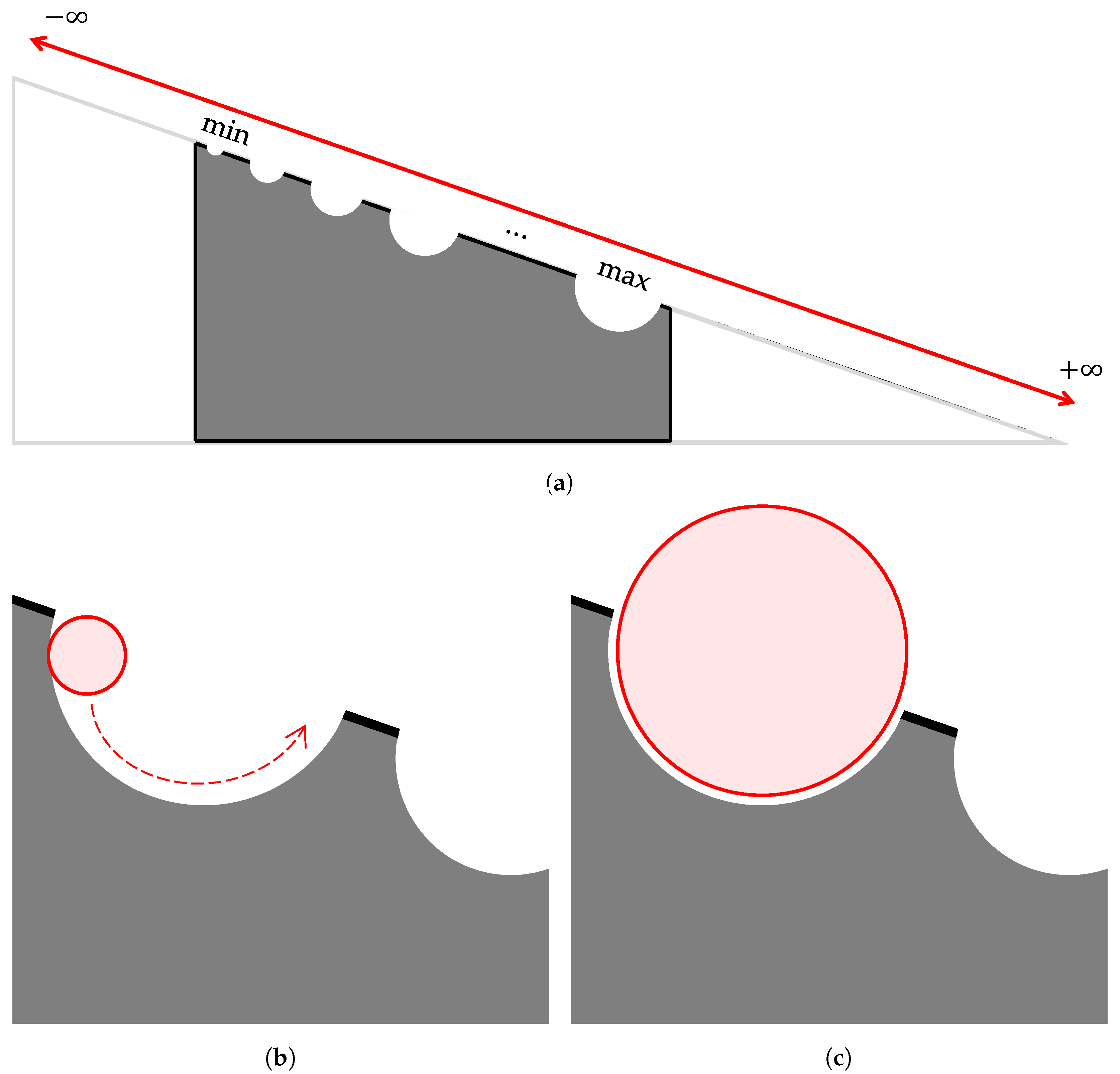
Appendix B. Min-Max Algorithm

The Min-Max Algorithm (refer to Algorithm A1) finds both the minimum and maximum of an integral list (linearly distributed) with n numbers in 3 n 2 = O ( n ) comparisons. A precise count for the number of comparisons can be found as follows:
  • For even n (i.e., n mod 2 = 0 ), one comparison is needed to initialize both the min and max. In pairwise processing, since the Algorithm starts from the third element of the list, the remaining n 2 elements are processed in pairs, and since n is even, n 2 2 is an integer. For each of these n 2 2 pairs, say x , y three comparisons are needed, one to compare a and b; one to compare the smaller of these with the min; and another to compare the larger of these with the max. In total, for an even n, 3 n 2 2 total comparisons are needed.
  • For an odd n (i.e., n mod 2 = 1 ), no comparison is needed to initialize the min and max, as they are set to the first element of the list. In pairwise processing, since the Algorithm starts from the second element of the list, the remaining n 1 elements are processed in pairs. For each of these n 1 2 pairs, again, three comparisons are needed. So, in total, for odd n, 3 · n 1 2 = 3 n 2 1 total comparisons are needed.
Algorithm A1 Pseudocode for Min-Max algorithm
Require: 
A list A n A i is the i’th element of the array, where n = | A n |
Ensure: 
Minimal and Maximal elements in the list A n
  1:
function MinMax( A n )
  2:
     i 0
  3:
     min , max ( NaN , NaN )
  4:
    if  n = 0  then
  5:
        return  ( min , max )
  6:
    end if
  7:
    if  n mod 2 = 0 then                                                 ▹Even number of elements
  8:
        if  A 0 < A 1  then
  9:
            min = A 0
10:
            max = A 1
11:
        else
12:
            min = A 1
13:
            max = A 0
14:
        end if
15:
         i = 2                                                                                 ▹Start from index 2
16:
    else                                                                        ▹Odd number of elements
17:
         min = A 0
18:
         max = A 0
19:
         i = 1                                                                                 ▹Start from index 1
20:
    end if
21:
    while  i n 2  do
22:
        if  A i < A i + 1  then
23:
            min = min ( min , A i )
24:
            max = max ( max , A i + 1 )
25:
        else
26:
            min = min ( min , A i + 1 )
27:
            max = max ( max , A i )
28:
        end if
29:
         i = i + 2
30:
    end while
31:
    return  ( min , max )
32:
end function

References

  1. Gonnet, G.H.; Rogers, L.D.; George, J.A. An algorithmic and complexity analysis of interpolation search. Acta Inform. 1980, 13, 39–52. [Google Scholar] [CrossRef]
  2. Manna, Z.; Waldinger, R. The origin of a binary-search paradigm. Sci. Comput. Program. 1987, 9, 37–83. [Google Scholar] [CrossRef]
  3. Chadha, A.R.; Misal, R.; Mokashi, T. Modified binary search Algorithm. arXiv 2014, arXiv:1406.1677. [Google Scholar]
  4. Thwe, P.P.; Kyi, L.L.W. Modified binary search Algorithm for duplicate elements. Int. J. Comput. Commun. Eng. Res. (IJCCER) 2014, 2. Available online: https://www.researchgate.net/publication/326088292_Modified_Binary_Search_Algorithm_for_Duplicate_Elements (accessed on 29 March 2025).
  5. Wan, Y.; Wang, M.; Ye, Z.; Lai, X. A feature selection method based on modified binary coded ant colony optimization Algorithm. Appl. Soft Comput. 2016, 49, 248–258. [Google Scholar] [CrossRef]
  6. Bajwa, M.S.; Agarwal, A.P.; Manchanda, S. Ternary search Algorithm: Improvement of binary search. In Proceedings of the 2015 2nd International Conference on Computing for Sustainable Global Development (INDIACom), New Delhi, India, 11–13 March 2015; pp. 1723–1725. [Google Scholar]
  7. Dutta, A.; Ray, S.; Kumar, P.K.; Ramamoorthy, A.; Pradeep, C.; Gayen, S. A Unified Vista and Juxtaposed Study on k-ary Search Algorithms. In Proceedings of the 2024 2nd International Conference on Networking, Embedded and Wireless Systems (ICNEWS), Bangalore, India, 22–23 August 2024; pp. 1–6. [Google Scholar]
  8. Perl, Y.; Reingold, E.M. Understanding the complexity of interpolation search. Inf. Process. Lett. 1977, 6, 219–222. [Google Scholar] [CrossRef]
  9. Shneiderman, B. Jump searching: A fast sequential search technique. Commun. ACM 1978, 21, 831–834. [Google Scholar] [CrossRef]
  10. Batir, N. Very accurate approximations for the factorial function. J. Math. Inequal 2010, 4, 335–344. [Google Scholar] [CrossRef]
  11. Olkin, I.; Pratt, J.W. A multivariate Tchebycheff inequality. Ann. Math. Stat. 1958, 29, 226–234. [Google Scholar] [CrossRef]
  12. Gesellschaft der Wissenschaften zu Göttingen; Georg-August-Universität Göttingen Nachrichten von der Königl. Gesellschaft der Wissenschaften und der Georg-Augusts-Universität zu Göttingen: Aus dem Jahre. 1884. Available online: https://gdz.sub.uni-goettingen.de/id/PPN252457072 (accessed on 29 March 2025).
  13. Jensen, J.L.W.V. Sur les fonctions convexes et les inégalités entre les valeurs moyennes. Acta Math. 1906, 30, 175–193. [Google Scholar] [CrossRef]
Figure 1. Pictorial representation of the Search-o-Sort theory.
Appliedmath 05 00064 g001
Figure 2. Infinitely long inclined plane (a), where the hypotenuse represents the ordered integral number system, Z , + . If the sphere falls in a hole of smaller radius, it will be thrown off by the inertial force (b), but will fit inside a hole of (nearly, as exact match might result in a toppling inertial force) the same radius (c).
Appliedmath 05 00064 g002
Figure 3. Graphical plots for the Sorting Algorithm, with intermediate search being performed by making use of Interpolation Search, Binary Search, Jump Search, and Linear Search, respectively.
Appliedmath 05 00064 g003
Disclaimer/Publisher’s Note: The statements, opinions and data contained in all publications are solely those of the individual author(s) and contributor(s) and not of MDPI and/or the editor(s). MDPI and/or the editor(s) disclaim responsibility for any injury to people or property resulting from any ideas, methods, instructions or products referred to in the content.

