Abstract
The biology literature addresses two puzzles: (i) the increase in specific metabolic rate of organs (SOrMR, W/kg of organ) with a decrease in body mass (MB) of biological species (BS), and (ii) how the organs recognize they are in a smaller or larger body and adjust metabolic rates of the body () accordingly. These puzzles were answered in the author’s earlier work by linking the field of oxygen-deficient combustion (ODC) of fuel particle clouds (FC) in engineering to the field of oxygen-deficient metabolism (ODM) of cell clouds (CC) in biology. The current work extends the ODM hypothesis to predict the whole-body metabolic rates of 114 BS and demonstrates Kleiber’s power law {}. The methodology is based on the postulate of Lindstedt and Schaeffer that “150 ton blue whale. and the 2 g Etruscan shrew.. share the same.. biochemical pathways” and involve the following steps: (i) extension of the effectiveness factor relation, expressed in terms of the dimensionless group number G (=Thiele Modulus2), from engineering to the organs of BS, (ii) modification of G as GOD for the biology literature as a measure of oxygen deficiency (OD), (iii) collection of data on organ and body masses of 116 species and prediction of SOrMRk of organ k of 114 BS (from 0.0076 kg Shrew to 6650 kg elephant) using only the SOrMRk and organ masses of two reference species (Shrew, 0.0076 kg: RS-1; Rat Wistar, 0.390 kg: RS-2), (iv) estimation of for 114 species versus MB and demonstration of Kleiber’s law with a = 2.962, b = 0.747, and (v) extension of ODM to predict the allometric law for maximal metabolic rate (under exercise, {}) and validate the approach for MMR by comparing bMMR with the literature data. A method of detecting hypoxic condition of an organ as a precursor to cancer is suggested for use by medical personnel
1. Introduction, Literature Review and Objectives
Recently, efforts are underway to link the fields of thermodynamics and combustion with biology in order to understand the virus evolution, develop empirical formulae for viruses, and analyze biological processes through Gibbs function and energy release within biological systems (BS) [1,2,3]. The current study extends previous work linking the field of oxygen-deficient combustion (ODC) with oxygen-deficient metabolism (ODM) [3] to: (i) predict the specific organ metabolic rates (SOrMRk) of vital organ k of mass mk (SOrMRk in W/kg of k, where k = Kidneys (Kids), Heart, Brain and Liver) for 114 BS ranging in mass from 0.0076 to 6650 kg, using organ mass (mk) data of all species and the SOrMRk of two reference species (RS-1 with lowest body mass, MB: Shrew, 0.0076 kg; RS-2 with MB,RS-2 > MB,RS-1 Rat Wistar, 0.390 kg; MB of RS-2 much higher than MB of RS-1), (ii) obtain the whole-body metabolic rates (BMR) of 116 species as a function of body mass (MB) by summing the organ metabolic rates (OrMRk) of individual organs (OrMRk = SOrMRk × mk) with known organ masses (mk) and (iii) demonstrate (a) Kleiber’s law for BS at rest and (b) the allometric law for maximal metabolic rate (MMR) during exercise. More importantly, the ODM framework introduces a dimensionless group (GOD)k for organ k for the biology literature to indicate the extent of OD within an organ.
1.1. Kleiber’s Law and Organ Metabolic Rates
Allometry refers to how the characteristics of biological species (BS), including morphological traits (e.g., brain size) and physiological traits (e.g., metabolic rate (MR), life span), change with body mass. The allometric relation for MR of BS is given as:
where MB is body mass (kg) and (), MR is in watts. In 1932, Kleiber obtained a = 3.4, b = 0.74 for MB ranging from 0.15 to 679 kg, known as Kleiber’s law [4,5], which persisted for over 70 years [6]. The specific basal metabolic rate (SBMR) is written as SBMR = , W/kg of body mass)
where b′ = b − 1 = −0.26. Nutrients consumed through the mouth are essential for energy release through oxidation. The review in Ref. [7] suggests that O2, which enters through nasal intake, must also be considered a “nutrient” since it is essential for energy release. The energy release rate (ERR) is related to the oxygen consumption rate within whole body since ERRB = , where HHVO2 is the higher heating or gross heating value per unit mass of oxygen consumed and it is almost constant at about 14,335 J/g of O2 for most fuels and nutrients [3]. Thus, the scaling function for metabolic rate with body size MB is explained with two existing theories:
- (I)
- If O2 supply from blood to the cells of tissues falls below a critical level , then its uptake is limited by the supply from blood vessels, which is a common assumption used in the classical WBE (West, Brown and Enquist) hypothesis [8] for demonstrating Kleiber’s law. West, a theoretical physicist, and ecologists Jim Brown and Brian Enquist proposed a fractal or “nutrient (including oxygen) distribution network” (i.e., the circulatory system of animal or vascular system of plants) hypothesis (also referred to as the “upstream” or supply side [9], or “outward-directed vascular network” [10]) and illustrated Kleiber’s law by minimizing the heart’s work required to pump a unit amount of blood; i.e., a network that minimizes the pressure difference (Paorta − Pcap). The scaling function is explained with O2 delivery to cells as the limiting factor.
- (II)
- Thermodynamics relates pressure losses (Paorta − Pcap) to entropy generation. Thus, Bejan [11,12], proposed that architectures and organs must develop in such a way that resistance to flow current (e.g., water flow in trees) must be minimized, or equivalently, that entropy generation is minimized, resulting in lower energy consumption and food requirements.
The biologists have raised the following issues as unknown: “The allometric size relationship is somehow ‘programmed’ into cells, although the factors that let them know whether they are in a small or large organism are still unknown” [13]. That is, existing biological data indicate that organs increase their metabolic rates per unit mass when within a smaller body and vice versa. In earlier work, the author proposed the “Oxygen-Deficient Metabolism (ODM)” or “downstream” hypothesis to explain these unknowns [3] and introduced a dimensionless group (GOD,k) for organs in the biology literature. In the current work, the same ODM hypothesis is extended to predict the whole-body basal metabolic rate as a function of MB for 116 BS and present a method of estimating (GOD,k) of organ k for use by the medical community.
1.2. Literature Review
While combustion is a rapid oxidation process that typically occurs at high oxygen mass fraction, YO2,air = 0.23 (mole fraction = 0.21 or 210,000 ppm), resulting in a significant temperature rise, the metabolism is a slow oxidation process that typically occurs at a low oxygen mass fraction, YO2 ( [3]) with a small rise in temperature rise for the body. The term pO2 is the partial pressure of O2 in mm of Hg. While the pO2 in the alveolar is 106 mm of Hg, the pO2 in tissues is about 40–50 mm Hg, and dissolved O2 is on the order of 2–5 ppm, thus resulting in a lower temperature rise in the body containing almost 50–75% water. Sometimes, the biology literature calls the energy release () as “heat produced” or “power produced” [14], while the engineering literature defines as the energy release rate (ERR) by all the cells within the body. The is a sum of the work delivery rate, , (i.e., ATP delivery rate, approximately 25% of ) and the heat transfer rate (, approximately 75% of , [15]) due to the temperature difference (ΔT) across the cells and the rest of the body.
The required O2 uptake (biology uses volume units in mL/min, in mg/min = 1.42 × ) by mitochondria in the cells is supplied by blood vessels via capillaries, followed by diffusion from capillaries to the cells immersed in the interstitial fluid (IF) and then from cells to mitochondria.
The hypotheses used for demonstrating Kleiber’s law { vs. MB} fall under two broad groups: (I) Homogeneous and (II) Heterogeneous.
- (I)
- Homogeneous hypothesis:
This hypothesis considers the whole body as a system; the hypotheses include: (i) the law of surface area to volume (S/V) ratio of the body, which balances the energy released over volume V with heat loss via skin to the ambience, yielding b = 2/3, b′ = −1/3, known as Rubner’s law (1883), (ii) WBE’s fractal geometry [8] (geometry of circulatory system: macro and microcirculation), which relies on minimization of dissipative energy in the vascular system supplying oxygen and nutrients. Savage et al. showed that the WBE model is applicable only for BS of infinite body size (or network) [16] and when finite size is included, it yields scaling exponents as a function of body size. Further, Weibel and Hoppeler [17] question the universal models based on “the fractal design of the vasculature and the fractal nature of the total effective surface of mitochondria and capillaries” since they predict b = ¾ for both basal and maximal metabolic rates. Silva et al. [18] suggest that there are mathematical and conceptual errors in network models, weakening the proposed theoretical arguments. The same review suggests that the power law exponent b should vary between 2/3 and 1 based on “metabolic level” (activity level of the organism or metabolic intensity). Painter et al. [19] agreed with the assumption of blood volume ∝ MB but questioned the assumptions of uptake nutrient consumption rate (called total current in the network) proportional to blood volume, (iii) Assuming the number of cells per kg body mass {ncell,m} in mammals is mass invariant, Ahluwalia [20] used the “downstream” hypothesis and Kleiber’s law {Equation(2)} to obtain a relation for the average cell metabolic rate (CMR, Watts/cell} as
and the reaction–diffusion equation with a source term was solved for two simplified cases: (a) Desorption controlled metabolism (zero-order kinetics): (Michaelis Menten constant) as in many in vitro samples {See Equation (16) in Ref. [3]}, and (b) adsorption controlled metabolism (first-order): . Ref. [20] presents results on MR in terms of Thiele Thiele modulus, ΨT. It was shown that b′ for the whole body satisfies the following bounds: −1/3 {high ΨT} < b′ < 0 {low ΨT} under first-order kinetics. Note that these bounds on b′ are given for the whole body while the ODM hypothesis presented in Ref. [3] presents Fk at the organ level {−1/3 < Fk < 0}; cf. Equation (7). Other models include (iv) network structures [10], (v) quantum mechanics [21], and (vi) topology [11].
- (II)
- Heterogeneous Hypothesis:
- A.
- Empirical Allometric Relations (EAR): The heterogeneous hypothesis considers the whole-body metabolic rate as a sum of the OrMRk with k = kids, H, Br, L and RM where RM represents all the remaining weakly metabolizing tissues. The mass of RM is given as
- (i)
- Body Mass Based Allometry: Wang et al. used a heterogeneous or reductionist approach for estimating the whole-body metabolic rate {} [22,23,24]:where is the SOrMRk of kth organ {W/kg of k} given by the body mass based allometry (BMA):
Here afterwards, this method of computing SOrMRk using the empirical allometric relations {EAR, Equation (4)} will be termed as EAR method. Wang et al. presented allometric relations for organ masses [23]:
Using Equations (4) and (5) in Equation (3), the is obtained as
Based on data on the organ mass and of six species (ranging from 0.48 kg of rat to 70 kg of human), Ref. [23] tabulates the constants ck,6, dk,6, ek,6 and fk,6. Table 1 tabulates the allometric constants ck,6, dk,6, ek,6 and fk,6 [23,24,25]. Since dk,6 > 0, organ sizes are positively related to MB, while the SOrMR (Equation (4)) are negatively correlated with body mass (fk,6 < 0). The additional subscript “6” indicates that the empirical constants are based on data from six species. Several other supporting data from references [26,27,28,29,30,31,32] are provided in footnotes of Table 1.

Table 1.
Allometric Constants for Organ Mass, Energy Release (Metabolic) Rate. Note: Values are based on six species: Rat (MB = 0.45 kg), Rabbit (2.5 kg), Cat (3 kg), Dog (10 kg), Human-1 (65 kg), Human-2 (70 kg). Constants ck,6, dk,6, ek,6, and fk,6 are from Ref. [23]; density from Ref. [24]). (Adopted and modified from Wang–5 organ model, Table 4 of Ref. [27]). . HHVO2 = 14,335 kJ/kg of O2 or 18.7 kJ/SATP L of O2 or 20.5 J/CST mL of O2 or 18.1 J/mL of O2 at 36.2 °C. HHVO2, kJ/L O2 for MB from 71 to 92 kg = 15.818 + 5.17 × RQ [32].
If one uses the data on ck,6 and dk,6 tabulated in Table 1, the resulting mass percentages (mk × 100/MB) for a 70 kg human are: 0.37% (Kids), 0.58% (Heart), 0.40% (Brains) and 1.90% (Liver), with the vital organ mass percentage at 3.25%. The corresponding energy percentages are 7.36% (Kids), 12.81% (Heart), 3.97% (Brain), and 17.10% (Liver), with the vital organ energy percentage at 41%. The RM for the 5-organ model is 66.2 kg, while the masses of Kids, H, Br, and L are 0.31, 0.33, 1.4 and 1.8 kg, respectively; this results in 94.5% of body mass being RM, while vital organs account for 5.5%. As opposed to a majority of BS, human brain masses are relatively larger, and the allometric relation underpredicts mBr for humans. Thus, human brain mass is estimated using the encephalization quotient (EQ), which is the ratio of measured brain mass to the mass predicted with allometry. Gallagher et al. report that for a reference human of 70 kg [33], brain mass is 1.4 kg while the brain mass is predicted as 0.28 kg from allometry indicating a high EQ. Vital organs contribute {mass % in parenthesis) 8.7% (0.4, Kids), 8.2% (0.5%, Heart), 21.6% (2%, Brain), and 20.2% (2.6%, Liver) of the total BMR [28]. The underprediction of human brain mass and energy percentage is due to the EQ factor, as humans have the highest EQ (i.e., a larger brain size compared to animals of similar mass). This additional brain mass enhances cognitive abilities beyond general brain mass versus body mass scaling laws.
- (ii)
- Organ Mass Based Allometry (OMA) Exponents for SOrMRk {or }: It is noted that “fk,6” in BMA for the vital organs of the six species in EAR by Wang et al. [23] are all negative. To explain the negative values of fk,6 in BMA for organs, and answer the puzzle on “how the organs inside the body know that they are in smaller or larger body and adjust the metabolic rates”, the BMA is replaced by organ mass-based allometry (OMA) using the relation between organ mass and body mass {Equation (5)} [3]. Thus,
See Table 1 for the listing of Ek,6 and Fk,6. The Fk,6 becomes more and more negative for increasing organ mass. Ref. [3] explains the rationale for Fk,6 vs. mk using the ODM hypothesis. It is apparent from the constant ek,6 and fk,6, or Ek,6 and Fk,6 that different organs consume oxygen at different rates, thus indicating different O2 profiles within IF. Since the ODM hypothesis is used to predict SOrMRk and demonstrate Kleiber’s law in the current work, a brief outline of Ref. [3] on ODC and ODM is presented below for the convenience of readers.
- B.
- Group or Oxygen-Deficient Combustion (GC or ODC) in Engineering: The engineering literature models the combustion of dense fuel particle suspension (e.g., coal suspensions fired into a boiler) using a spherical fuel cloud (FC) of radius RFC, mass mFC and number density of fuel particles nFC, with its surface exposed to a known oxygen mass fraction at the surface YO2,FC,s. Each particle located at “r” from the center of the spherical cloud is subjected to YO2(r) and consumes oxygen at the rate of :where the characteristic oxygen consumption rate by the particle, Cch,p, and the relation for Cch,p changes depending on kinetics control (CCh,p = CCh,p,kin) with a first-order reaction, or diffusion control (CCh,p = CCh,p,dif). The basic relations for Cch,p are given in Ref. [3]. A detailed description, along with engineering results for (i) O2 consumption rate of the whole cloud and (ii) effectiveness factor {ηeff,FC} for a spherical FC, are presented in Refs. [3,34] in terms of dimensionless group G; they are briefly presented here.
The solutions for , are presented in terms of the effectiveness factor (ηeff,FC) of the FC, which is defined as a ratio of the O2 consumption rate by all particles within the cloud to the rate of consumption of O2 in the case that each particle within the FC is subjected to YO2,FC,s:
where the energy release rate , and the specific energy release rate . Using oxygen profiles YO2(r) within the cloud, the relation for ηeff,FC is given as:
The dimensionless group G for FC is defined as:
and the G number for FC is shown to be related to Thiele Modulus, ΨT (G = ΨT2) in the porous char combustion literature [28,29]. Using Equation (10), the effectiveness factor can be plotted against G as shown in Figure 1. It is noted that G ∝ RFC2, and since the mass of the fuel cloud, mFC ∝ RFC3 and hence G ∝ mFC(2/3), assuming a constant number density of fuel particles (nFC). The caption of Figure 1 describes the results for ηeff,FC vs. G for the fuel clouds.
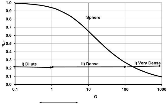
Figure 1.
Effectiveness Factor of organ k (ηeff or ηeff,k for organ k in biology) vs. G (or GOD,k for application to cell clouds in biology). For application to an organ k in a BS, particles are replaced by cells in the ODM model. (I) Dilute Cloud: G or GOD,k < 1, within which ηeff ≈ 1, indicating all particles are exposed to the same surface oxygen concentration, or each particle releases energy as though it is isolated. (II) Dense Cloud: Interactive Combustion Mode or ODC mode with a decreasing oxygen concentration within the cloud, 1 < G or GOD,k < 100, (III) Very Dense Cloud: G or GOD,k > 100. Particles near the surface oxidize rapidly, while the center of the cloud contains very little oxygen, and particles at the core may not oxidize. The same plot is valid for cell clouds with ηeff, = ηeff,k, G = GOD,k. (I) Dilute Cell Cloud: GOD,k < 1, within which ηeff ≈ 1, indicating all particles are exposed to same surface oxygen concentration, or each cell releases energy as though it is isolated. (II) Dense Cell Cloud: Crowding effects of cell or ODM mode with a decreasing oxygen concentration within the cloud, 1 < GOD,k < 100. (III) Very Dense Cloud: GOD,k > 100. For this zone, .
- A.
- Oxygen-Deficient Metabolism (ODM) in Biology: The oxygen diffuses from capillaries towards the metabolic cells contained within interstitial fluid (IF). Even though the biology literature suggests a radial diffusion distance of the order of 100 μm (where pO2 ≈ 0) from the capillaries, the actual path may be longer, leading to a decreased O2 transport rate (or decreased effective diffusivity) to the mitochondria. The diffusive O2 transport rate is affected due to the following [35,36]: (i) closely packed cells (number density of cells, n, or crowding effect) [13] (ii) tortuous oxygen path, (iii) amount of aqueous fluid, (iv) extracellular structures or cell barriers, and (v) presence of cytoplasm (which alone reduces D by 30 times the normal level). As a result, cells far away from the capillaries cannot maintain the required O2 flow for ATP production [37] leading to oxygen deficiency (OD).
- B.
- ODM in Organs and Significance: Hypoxic conditions (low pO2 in cells) decrease the oxygen consumption rate by cells, while anemic conditions or a reduction in blood flow [38] or reduced Hb contents cause a decrease in O2 supply to the cells from capillaries. Hypoxic conditions cause a reduction in ATP production rate, leading to “bioenergetic collapse” [39]. These conditions lead to sleeper cells. The OD in cells results in the production of protein called HIF-1α (hypoxia-induced factor), a dimeric protein complex that causes a metabolic shift from oxidative phosphorylation (OXPHOS) to glycolysis. HIF enables the activity of genes to switch from oxidative phosphorylation to glycolytic pathways [40] for energy and ATP release. ODM promotes a switch to glycolysis, where only two ATP are obtained per CH compared to 32 ATP via oxidative phosphorylation, resulting in a decrease in overall energy release [41] and rapid cell division due to more intermediaries provided by glycolysis which serves as a source of energy for cancer cells [42]. It is well known that oxygen deficiency (OD) or hypoxia contributes to several diseases, including cancer, stroke, anemia, and heart disease. There appears to be a positive correlation between the mass of an organ and the number of cancer cases [43], which is attributed to the link between excess fat in organs and obesity.
- C.
- Modeling ODM in Cell Clouds:
- (i)
- Phenomenological type of ODM Model: Singer et al. studied the role of OD or the “crowding effect” on the metabolic rates of in vitro organ samples and developed a phenomenological type of model [44]. Just like particles in FC, the cells near the aerobic surface undergo high SOrMRk while those cells near the anerobic core may undergo only glycolysis. Recently, Botte et al. [45] dealt with the effects of cell packing on O2 consumption within densely packed cells of 3D cultures. They introduced proximity index (PI, a measure of cell–cell interaction), an uptake coefficient (ϕ, a measure of area around the cell through which O2 passes), and dimensionless group called LSU (local supply to uptake ratio = ϕ/D), which is similar to GOD. They studied the effects of cell packing medium on CMR and used LSU to correlate CMR. In the author’s opinion, LSU may be called LUS (local uptake to supply via diffusion), which also aligns with engineering interpretations of GOD,k {cf. Equation (14)}.
- (ii)
- Detailed ODM Model following ODC Literature in Engineering: More detailed ODM models were developed by Annamalai by adapting the ODC literature from engineering to biology [3]. Unlike the Krogh cylinder model, where the capillary is placed on the axis (COA) of a cylinder containing metabolic cells within IF, the ODM model uses a spherical cloud of cells (CC) of radius RCC having nCC, cells per unit volume with capillaries on the surface (COS) of CC with mass of CC, mcc {Figure 2a}. The COS model is also known as the “solid cylinder” model in biology when geometry for modeling uses cylindrical geometry [46]. A detailed comparison between ODC and ODM models, and relations for several variables of interest, are presented in Ref. [3]. In ODM, the fuel cloud is replaced by a cell cloud (CC), particles are replaced by cells of the organ k in BS, and YO2,FC,s becomes YO2,CC,s. The radius RFC is replaced by RCC, the ERR is replaced by the organ metabolic rate (OrMRk) and SERR is replaced by SOrMRk in cell clouds, defined as SOrMRk = (OrMRk)/mCC}k. The G number in engineering [47]) is also replaced by GOD,k for organ k. The oxidation rate for each particle is replaced by the cell metabolic rate {Figure 2d}. These relations will be summarized in the Section 2.2.
Just like FC, there exists three zones of operation of CC: (I) Dilute {GOD,k < 1, ηeff,k ≈ 1, Fk based on OMA ≈ 0, ηeff,k ≈ 1}, (II) Dense Cloud {1 < GOD,k < 100, ηeff,k < 1}, Fk < 0 and (III) Very dense Cloud {GOD,k > 100, {e.g., Liver}, ∝ mk(−1/3) or Fk → (−1/3) as GOD,k becomes large}. More details for CC model are provided in the caption of Figure 2. Those cells near the surface are aerobic with a higher rate of oxidation of nutrients, while those cells near the core of the cloud are anaerobic with very little oxygen. Cells near the core may undergo only glycolysis {Figure 2b} leading to the production of protein HIF-1α.
While resting, limited capillaries are perfused with blood (Figure 2b, surface at YO22,cc,s), whereas under exercise, almost all the capillaries are perfused (Figure 2c) increasing YO22,CC,s at the surface of CC {e.g., Maximum Metabolic Rate (MMR) when there is increased blood flow through selected organs during exercise}.
The literature review suggests that despite several hypotheses outlined in Section 0 for the 3/4 law, “the hunt for an explanation of the 3/4 law continues” [48]. The current ODM hypothesis focusses on the metabolic rate he controlled by “downstream demand-side” oxygen consumption of all the cells within an organ and provides another “hunt” for an explanation of the 3/4 law.

Figure 2.
(a) Capillary system: Cells can be placed within a cylinder with capillary on axis (COA, Figure 2a) or cells can be enclosed by capillaries on surface (COS). The (COS) model is known as the solid “cylinder” model in biology for a cylindrical geometry (Figure 2a) [49] (b) COS model for spherical cloud of cells subjected to fixed oxygen mass fraction at the surface YO2,CC,s with cell located at “r” consuming O2 at the rate of ; capillaries are partly perfused. The effective area for O2 exchange is limited since only 25% to 35% of available capillaries are perfused under BMR conditions [50] {e.g., resting conditions resulting in lower YO2,CC,s}. (c) COS model with mostly perfused capillaries {e.g., exercise, resulting in higher YO2,CC,s} for a spherical cloud of cells. (d) Oxidation at cell level with local YO2(r) supplying oxygen to the cell and nutrients oxidized to CO2 and H2O. COS model is close to ODC model in the engineering literature. The O2 diffuses towards the center of cell cloud (CC) of radius RCC and mass mCC. Cells adjacent to the surface containing capillaries are aerobic, while those farther surfaces become hypoxic, and the farthest cells are necrotic cells. Detailed results for cell clouds are given in Column 4 of Table 2 in Ref. [3] Certain regions within organs may undergo only glycolysis due to a lack of O2. note that for the partly perused capillaries as shown in (b) YO2,CC,s. (d) Single cell within IF with diffusion of O2, oxidation and release of CO2 and H2O. During exercise, capillaries are mostly perfused (Figure 2c).

1.3. Objectives
The objectives of the current work are to (i) link the field of group or oxygen-deficient combustion (ODC) in engineering with the field of oxygen-deficient metabolism (ODM) in biology, (ii) adopt the relations developed for energy release rate per unit mass (SERR, W/kg fuel cloud) to predict SOrMRk (W/kg of organ k) of 116 BS ranging in body mass from 0.0075 to 6650 kg, using known organ mass data (mk) and SOrMRk of two BS, referred to as Reference Species (RS), where RS-1 has the lowest body mass, MB,RS-1 (Shrew, 0.0075 kg, ηeff,k ≈ 1), and RS-2 has a much higher body mass, MB,RS—2 >> MB,RS—1 (Rat Wistar of 0.390 kg, ηeff,k < 1), (iii) estimate the whole-body metabolic rate versus MB by summing the predicted organ metabolic rates, and validate the ODM method by demonstrating Kleiber’s law for BS at rest with an exponent close to 0.75, (iv) predict an hypothetical upper metabolic rate (UMR) for organs, and, consequently, for the whole body, assuming all cells within each organ metabolize without oxygen concentration gradients; (v) obtain the maximal metabolic rate (MMR) during exercise, when most of the capillaries at the cell cloud surface are perfused, and show that the whole-body allometric law under exercise yields an exponent close to 0.87, as reported in the literature; (vi) suggest methods of estimating GOD,k and hence extent of OD in organs for use by medical personnel.
2. Materials and Methods
2.1. ODM Hypothesis
The ODM hypothesis assumes that each organ k consists of multiple cell clouds (CC), with each cell cloud having a mass mcc,k and radius RCC,k, which is related to the organ mass mk by RCC,k α mk1/3. It is also possible that capillaries do not fully cover the entire spherical surface enclosing the cells (Figure 2b). Typically, 25–35% of an organ’s capillaries are perfused at rest, with perfusion increasing during exercise since there is increased metabolic demand; further a higher perfusion percentage results in a higher YO2,cc,s. The effective area for O2 exchange is limited, since only a fraction of capillaries on surface are perfused under BMR conditions [50], which affects the O2 diffusion distance and, hence, the metabolic rate within the organ. Using the Krogh–Erlang equation, Ostergaad demonstrated that only 10% of SM capillaries are perfused at rest, but more capillaries are recruited during exercise [51]. Further details can be found in Section 2.2 and Section 3.4.
Smaller species have smaller organs (e.g., shrew of mass 0.0075 kg), while larger species have larger organs, as indicated by dk > 0 in the allometric exponents for organ sizes (Table 1). Thus, the smaller organs of smaller species may have shorter distances for O2 diffusion from capillaries to cells, allowing metabolism to occur as if each cell within the CC is exposed to the same O2 concentration as YO2,CC,s (ηeff ≈ 1), resulting in SOrMRk of RS-1 ≈ SOrMRk,iso, of same organ k of any BS. However, isolated cell metabolic rates can still vary from organ to organ, even in smaller species, due to differences in functional requirements, cell reactivity, and O2 transport rate (e.g., heart tissues containing Mb can deliver O2 at a faster rate resulting in increased effective transport coefficients for O2 from capillaries to mitochondria). As organ mass increases (e.g., in the liver), ηeff,k < 1, and SOrMRk ≈ ηeff,k × SOrMRk,iso, where it is assumed that for any given organ k, SOrMRk,iso remains the same for all BS regardless of body size.
2.2. Methodology
Detailed comparisons of the governing conservation equations, and several relations for various parameters in the fields of ODC in engineering and ODM in the biology literature are presented in Ref. [3]. These include: (i) conservation equations for both fields, (ii) the ERR of a single particle in a FC and a single cell in a CC in terms of YO2, (iii) oxygen profiles in FC versus CC, (iv) the dimensionless number G for FC and GOD,k for the CC of organ k and (v) the SERR of FC (W/kg of cloud) in terms of the effectiveness factor and G and specific organ metabolic rate (SOrMRk) of CC (W/kg of cell cloud of organ k) in terms of the effectiveness factor ηeff,k and GOD,k. The methodology and relevant relations for the current work are briefly summarized below.
- (i)
- Metabolic Rate of single cell located at r in CC {Figure 2}where CCh,cell, characteristic cell O2 consumption rate {W/kg cell} when YO2 = 1; the relations for CCh,cell under first-order kinetic control or diffusion controlled O2 consumption rates are given in Ref. [3] in terms of kMM constants, transport properties and cell diameter.
- (ii)
- Oxygen Profiles within CC
Adopting the engineering literature [34], the profile for oxygen mass fraction within the cell cloud of organ k, is given as {See Table 3, items 10 and 11 in Ref. [3]}.
where for organ k
where RCC,k ∝ mk1/3, Cch,cell, characteristic O2 consumption rate of cell. Note that GOD,k = ΨT,k2 where ΨT,k is called Thiele Modulus in porous char oxidation literature [28]. The larger the radius RCC,k or organ mass mk, the higher the GOD,k or ΨT,k, and the characteristic O2 consumption rate by cell cloud. The term is the characteristic consumption (or uptake) rate by CC, and characteristic diffusion rate from the CC surface to the CC. The GOD,k is almost similar to LUS (defined as local uptake to supply ratio) presented in Ref. [45]. It is noted that lowest mass fraction of O2 is at the center of the CC with . The higher the consumption rate of O2 compared to supply via diffusion, the higher the GOD,k, the lower the YO2(0), and the lower the ηeff,k and vice versa..
- (iii)
- Effectiveness Factor of Spherical CC and Specific Organ Metabolic Rate {SOrMRk}
Adopting the same procedure as in engineering,
With YO2 profile from Equation (13), the ηeff,k is derived as:
where k = Kids, H, Br, and L Using the definition of ηeff,k, the SOrMRk is given as
where . Equation (17) reveals that SOrMRk is a function of GOD,k in biology. One may classify the CC as dilute, dense and very dense clouds: (I) Dilute CC: GOD,k < 1, ηeff,k ≈ 1 (Figure 2, ηeff, replaced by ηeff,k, G replaced by GOD,k). For Zone I, Equation (16) leads to ηeff,k =1 and hence . Thus, in OMA, Fk → 0 for smaller organs, e.g., Fk for Kidney is −0.094, (II) Dense CC: 1 < GOD,k < 100. As the organ size increases, mass increases, GOD,k increases, ηeff,k the effectiveness factor of organ k decreases. (III) Very dense CC, or Sheath CC: GOD,k > 100 (e.g., Liver, a large organ), ηeff,k is very low and [34]. Since GOD,k ∝ RCC,k2 ∝ mk(2/3); Thus . Fk in the organ mass based allometry (OMA, Equation (7)) becomes −1/3 for large organs (e.g., Liver). The ODM hypothesis leads to the bounds: −1/3 < Fk < 0 for vital organs. The data for liver, a large organ shows that Fk = −0.31 while Fk = −0.094 for Kidney, a smaller organ (Table 1).
- iv
- Metabolic Rate of Vital organs {}: Using Equation (17) for the vital organs, the metabolic rates of vital organs of any BS:where , k = kid, H, Br and L.
- v
- Metabolic Rate of Remaining Mass (RM) of Tissues {} for any BS
The remaining mass of organs (RM) represents a sum of all “minor”(i.e., weakly metabolizing) organs (e.g., SM, skin, Adipose Tissue, etc.) within the body, and the specific metabolic rate of RM (W/kg of RM) is needed. There are several possible approaches: (a) Select data for each of minor organ if available, estimate the effectiveness factor for all minor organs, and adopt a similar procedure outlined for vital organs, (b) Use the EAR for RM: ; from Table 1, eRM,6 = 1.45, fRM,6 = −0.17, in W/kg, (c) Assume Elia’s constant values for as 0.581 W/kg for all BS. In the current work, methods (b) and (c) are adopted for estimating .
- vi
- Whole Body Metabolic Rate () under Rest
Adopting the heterogeneous method, the whole body metabolic rate under rest, {} is given as
- vii
- Metabolic Rate of RM {} and Whole-Body Metabolic Rate {} under Exercise
During exercise, blood flow to the skeletal muscle (SM) is increased to supply the required oxygen and nutrients. Thus, SM becomes metabolically more active compared to other tissues within the RM due to increased capillary perfusion, increasing from approximately 25% at rest to nearly 100% during exercise.
Relations for depends upon the YO2,CC,s and hence the percentage of capillaries perfused. The remaining mass of tissues under exercise is given as
where is different from under rest due to the percentage of capillaries perfused under exercise are different from those at rest. The during exercise is given as,
- viii
- Upper Metabolic Rate (UMR, ) and Maximum Metabolic Rate (MMR, ) of Whole Body
- (a)
- UMR: The Upper metabolic MR of organ k (not the maximum MR) and hence, the whole-body MR can be estimated by setting ηeff,k = 1 for all organs {i.e., no oxygen gradients within CC}, including RM.
- (b)
- MMR: When the CC surface is covered with more perfused capillaries, the YO2,CC,s increases, and most of the cells are aerobic, resulting in the MMR, and leading to a whole-body allometric law with an exponent higher than 0.75. The MMR is obtained for two cases: (a) Lower limit on MMR by keeping O2 gradients but accounting for more perfusion on CC surface; (b) upper limit on MMR by setting ηeff,k = 1 (i.e., no O2 gradients, setting ηeff,k = 1 for all organs, including SM, and RM,Ex) during exercise. The percentage of capillaries perfused under rest and exercise conditions is shown in Table 2. The percentage of perfusion affects YO2,CC,s. The change in YO2,CC,s is given by the following relation:
The increased YO2,CC,s causes isolated rates to increase (i.e., higher, thereby increasing the whole-body metabolic rate. Note that the blood flow rate to organ k is given by the product of % blood flow to organ k* circulation rate of blood/100. The pumping rate of blood by the heart changes depending on the resting or exercise conditions, leading to a whole-body allometric law with an exponent higher than 0.75.
Table 2.
Capillary Perfusion Under Rest and Exercise. Note: Capillary perfusion percentage does not affect SOrMRk and BMR estimations; they affect only YO2,CC,s or MMR under exercise. In ODM method [49]. Cardiac Output = 5.8 (rest), 9.5 (m ild exercise), 17.5 LPM (maximal exercise). Vital Organ Blood flow: 2.7 (Rest), 2.4 (Mild Exercise), 2.5 LPM (Maximal Exercise). Vital Blood Flow %: 47 (Rest), 25 (Mild Exercise), 14 (Maximal Exercise). (Vital Blood flow)Ex/Vital Blood flow)Rest = 1 (Rest), 0.89 (Mild Exercise), 0.93 (Maximal Exercise).
| Organ | Rest (mL/min) | Mild Exer (mL/min) | Maximal (mL/min) | Rest % | Max. Exercise % | Max Ex/Rest Ratios |
|---|---|---|---|---|---|---|
| Kidney | 1100 | 900 | 600 | 19.0 | 3.4 | 0.55 |
| Heart | 250 | 350 | 750 | 4.3 | 4.3 | 3 |
| Brain | 750 | 750 | 750 | 12.9 | 4.3 | 1 |
| Others (i.e., liver, spleen) | 600 | 400 | 400 | 10.3 | 2.3 | 0.67 |
| Skeletal muscle | 1200 | 4500 | 12,500 | 20.7 | 71.4 | 10.42 |
| RM, Ex (GI + skin + others) | 2500 | 3000 | 2900 | 32.8 | 14.3 | 1.32 |
2.3. Estimation of OD Number (GOD,k) and Specific Organ Metabolic Rate of Organ k {SOrMRk} of Any BS
Equation (16) presents ηeff,k in terms of the dimensionless number GOD,k. If GOD,k of an organ is known, then ηeff,k can be estimated; or, if the actual MR of an organ under interactive and isolated modes is known, so that ηeff,k can be estimated, then GOD,k can be solved. The predictions on SOrMRk of organs require the estimation of GOD,k of each organ of 116 species; difficulty arises in the estimation of GOD,k {See Equation (14)} since it requires a knowledge of (i) the reactivity of cells within organ k undergoing metabolism (CCh,cell) either under diffusion or kinetic control, (ii) the overall transport coefficient D of oxygen from capillaries to mitochondria, (iii) capillary number density, cell cloud radius which may change within an organ k and (iv) percentage of capillaries perfused for each organ in the 116 BS, which affects (YO2,CC,s)k. Two methods are proposed for estimating GOD,k and SOrMRk of organs:
- (A)
- Basic Method: This approach requires basic data for CCh,cell, D, % of capillaries perfused for each organ k. These properties may vary by an order of magnitude. Consequently, greater uncertainty exists in the estimation of GOD,k and SOrMRk due to variations in these parameters across the organs of 116 species.
- (B)
- Ratio Method or Reference Species (RS) Method: To circumvent the data collections, minimize the wide variations in properties and reduce the uncertainties, the current work proposes references species (RS) method, also known as the ratio method. Two reference species are selected: RS-1 is selected as the BS with the lowest body mass (e.g., Shrew, MB = 7.6 g with ηeff,k ≈ 1), and RS-2 is selected as a BS with significantly higher body mass (e.g., Rat Wistar, MB = 390 g, almost 50 times heavier than that of RS-1; so ηeff,k < 1). The method is based on the premise that the metabolic behavior of organ k of BS with the lowest body mass is close to “isolated” rate with almost no oxygen gradient because of very few cells within the organ k; i.e., all cells are at YO2,CC,s, and hence ηeff,k ≈ 1. Then the isolated metabolic rate of organ k of any other BS since basic architecture of cell is same for almost all mammalian species. Justification is as follows. Makarieva et al. [52] demonstrated that SBMR varied from 0.3 W/kg to 9 W/kg (a 25-fold variation), despite a 1020-fold difference in body mass for “bacteria to elephants and algae to trees”. Then it follows that the cell metabolic rate (CMR) does not vary significantly across BS, since the number of cells per unit mass is similar across BS. This view is confirmed by Lindstedt and Hoppeler [53], who stated that the “150-ton blue whale”, which is 75 million times the mass of the 2 g Etruscan shrew, “shares the same architecture… organ systems, biochemical pathways”. For RS-2, the GOD,k falls within the dense zone (i.e., the steeper part of ηeff,k vs. GOD,k, Zone II in Figure 2); hence (ηeff,k)RS-2 < 1. With the known SOrMRk data for RS-1 and RS-2, (ηeff,k)RS-2 is estimated as
The corresponding (GOD,k)RS-2 is evaluated using Equation (16). This RS method reduces uncertainty in the results by relying on ratios, thus canceling out the effects of several biological properties. With the assumption of a constant cell diameter for a given organ k across BS [16], constant number density of cells and using the definition of GOD,k (Equation (14)), GOD,k ∝ RCC,k2 and since the mass of the cell cloud, mCC,k ∝ RCC,k3, then GOD,k ∝ mCC,k2/3 ∝ mk2/3. Knowing the organ masses for any BS (other than RS-1 and RS-2), the GOD,k values can be estimated using the following relation:
And the corresponding ηeff,k is estimated using Equation (16). Thus, the SOrMRk for k = Kids, H, Br and L, , and , are determined from Equation (17), Equation (18), and Equation (19), respectively. Note that the RM consists of several organs with metabolically weak cells. Hence is estimated by two methods: (I): Body mass based EAR (Table 1, [23]); (II) Elia’s constant for SOrMRRM (Table 1). Finally, can be estimated from Equation (20), with the known organ masses of 116 species. Results are presented in the next section. A step-by-step procedure is presented in the Supplementary Materials A placed on MDPI website.
3. Results and Discussion
The results are presented in the following order: 1. (A) EAR for all organs and (B) EAR for vital organs with Elia’s constant used for RM, 2. (A) ODM for vital organs with EAR for RM, and comparison with results from the EAR for all organs [23], (B) ODM for vital organs with Elia’s constant for RM (C) effects of changing the selection of RS-2 on ODM results 3. Comparison of the energy contribution percentage by vital organs using the ODM method versus the EAR method, 4. (A) Allometric constants for the upper metabolic rate (UMR), assuming no oxygen gradients within organs (B) Allometric constants for the maximum metabolic rate (MMR), based on known perfusion percentages at rest and during exercise (Table 2), with comparisons to literature data.
3.1. Whole Body Metabolic Rate Using EAR for All Organs and the Effect of Elia’s Constant for on Whole-Body Allometry
- A.
- Empirical Allometric Relations (EAR) for all Organs: Wang et al. [22] used the EAR constants (Table 1) for all organs of 116 species in estimating the SOrMRk, then summed up the OrMRk {=SOrMRk * mk} with known organ masses to obtain the whole-body metabolic rate () and plotted vs. MB {Figure 3}, which yielded Kleiber’s law with a = 3.216 and b = 0.756. Table A1 in Appendix A tabulates the body mass, organ masses, and with EAR method for al organs (last column, Table A1) for 116 species.
- B.
- EAR for Vital Organs and Elia Constant for RM: In order to study the effect of using EAR for RM, the author replaced the EAR for RM with Elia’s constant for RM { of 0.581 W/kg} and computed the whole-body metabolic rate. The constants in Kleiber’s law become a = 2.486 and b = 0.781 (Figure 3). It is seen from that that the slope b increased from 0.76 to 0.78, representing a 3.31% increase in the exponent b indicating that the slope “b” is dominated by vital organs.

Figure 3.
Comparison of Kleiber’s Law {} using EAR for all organs with the Kleiber’s law with EAR for vital organs and Elia constant for RM. (a) The BMA allometric constants in SOrMRk relations were derived from organ metabolic rate data of six species ranging in mass from 0.48 kg to 70 kg [21]. By extending these same organ allometric constants to 116 species and using available organ mass data for these species (ranging from 0.0075 kg to 6650 [20]), the resulting allometric constants using EAR for all organs were a = 3.216 and b = 0.756. (b) With EAR for vital organs and Elia’s constant for RM, { = 0.581 W/kg}, the estimated allometric constants were a = 2.489 and b = 0.781. A minority view holds that the b for BMR is approximately 0.67 [54], rather than the widely accepted value of 0.75.

3.2. Whole Body Metabolic Rate Using ODM Hypothesis and Comparison with Results from EAR Method
- (A)
- ODM and EAR for SOrMRk of RM: The ODM model uses the relation for effectiveness factor of four vital organs to predict SOrMRk and using the allometric law for . Figure 4 shows the results for the whole-body metabolic rate {} vs. MB obtained.
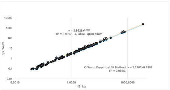 Figure 4. Comparison of whole-body metabolic rate using the ODM and Reference Species (RS) Method {RS-1: Shrew MB = 0.0076 kg; RS-2: Rat Wistar = 0.390 kg} with EAR for all organs; , MB = 0.0075 kg to 6650) (i) (⬤)ODM Method: Vital Org with ηeff and RM follow EAR, a = 2.963, b = 0.747, (ii) (O) EAR Method for all organs: a = 3.216, b = 0.756. Kleiber’s law constants are almost the same with both methods.
The same figure provides a comparison with Wang’s results using EAR. Note that the ODM method relies only on data from two reference species, RS-1 and RS-2, to predict SOrMRk and whole-body metabolic rates for the remaining 114 species. The current ODM method for estimating SOrMRk is validated, as it supports Kleiber’s law.
Table A1 compares the ODM-based metabolic rate, for 116 species with those using the EAR method (last two columns). If the error percentage is defined as {MR with ODM–MR with EAR) × 100/MR with EAR}, then the highest error occurs for a 60 kg human at 24.07%. The average error across all 116 species is 8.14%.
- (B)
- ODM for Vital Organs and Elia’s Constant SOrMRk for RM: When the SOrMRk of vital organs from the ODM method and Elia’s constant for RM are used, a = 2.242 and b = 0.772. The results show that the allometric constant b increases from 0.747 to 0.781 (Figure 5), indicating 3.35% increase in the slope of b. This increase in b is nearly the same as in the EAR method (Section 3.1). The residual mass (non-vital mass) seems to play a minor role in determining the exponent b, since the vital organs are more metabolically active. It is apparent from Figure 4 and Figure 5 that the current ODM method for the estimation of SOrMRk is validated, as it supports Kleiber’s law.
- (C)
- Effects of Change in Selection of RS-2 species in ODM method: When BS of masses of 337 g {45 times MB of shrew, 0.86 times MB of Rat Wistar} and 84 g {11 times MB of shrew, 0.21 times MB of Rat Wistar} were selected for RS-2, the “b” changes by 0.1% and −0.12%, respectively, indicating a negligible change in “b”.

Figure 5.
Effects of Energy release from RM on Kleiber’s law using ODM method. Based on 116 BS with MB from 0.0075 to 6650 kg: (i) Vital Organs under ODM and RM following EAR: a = 2.963 b = 0.747, (ii) Vital Organs under ODM and RM with Elia’s constant of 0.581 W/kg: a = 2.242, b = 0.772. The percentage increase in b for the ODM method is the same as the percentage increase in the EAR method.

3.3. Vital Organ Contribution Percentage with ODM Method and Comparison of Results with Empirical Allometric Relations (EAR) Method
As a further validation of the ODM method, the predicted percentage contribution of vital organs is compared with literature data. Figure 6 shows the computed ERR from the four vital organs vs. mvit, while Figure 7 compares the percentage energy contribution of vital organs estimated using ODM with those obtained using EAR. If the allometric fit for is expressed as with in watts, mvit in kg, and vital energy contribution as , the fits yield αvital = 12.69, βvital = 0.74, γvit = 51.85, νvil = −0.115, while the previous literature with the EAR method for all vital organs suggests αvit = 15.67, βvit = 0.77. γvit = 49.67 and νvil = −0.101 [23]. The energy contribution estimated from ODM appears to agree with data from the EAR method for MB up to 500 kg. The OD in organs results in a slope of vs. mvit that is less than 1, indicating the increase in is less than proportional to the increase in the vital organ masses.
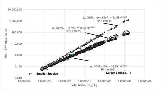
Figure 6.
The metabolic rate from vital organs (Vital ERR) and UMR (ηeff,k = 1 for all vital organs) as a function of vital organ mass, mvit: Comparison between ODM and EAR data. Vital organ MR (ODM) for 116 BS with body mass ranging from 0.0076 kg to 6650 kg; , in watts, mvit in kg. (a) (■) ODM Method: αvit = 12.961, βvit = 0.737, (b) (O) EAR Method: αvit = 15.667, βvit = 0.767. Note that under ODM are slightly lower compared to of EAR. (c) in watts when O2 gradients disappear for all vital organs (ηeff,k = 1 for all vital organs) (▲): , αvit,UMR = 92.58, βvit,UMR = 1.009. There is jump in αvit,UMR from 15.67 to 92.58 and βvit,UMR from 0.737 to 1.008 when gradients disappear. For , the law is almost isometric with respect to vital organ mass since all cells in vital organs are exposed to uniform cloud surface oxygen concentration.
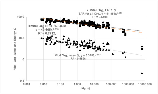
Figure 7.
Comparison of vital organ mass % and energy % vs. MB. Allometric Fit, . From ODM method (■): γvit = 49.67, νvil = −0.115. EAR for all vital organs (⬤) [23]: γvit = 51.85, νvil = −0.101. (▲) Vital organ mass % = 45.376 MB−0.141.
3.4. The Upper Metabolic of Whole-Body {UMRB} and Maximum Metabolic Rate of Whole-Body {MMRB}
The ηeff,k is a function of oxygen gradients within cell clouds; the steeper the gradients lower is ηeff,k. The of any BS is a strong function of SOrMRk {=ηeff,k }, and is affected by YO2,CC,s, which depends on the percentage of capillaries perfused at the CC surface. Equation (20) states that whole-body metabolic rate {} increases with the increase in ηeff,k {i.e., } for metabolically dominant vital organs and the remaining tissue masses.
- (A)
- Hypothetical Upper Metabolic Rates of Organs and whole body: The resting or basal metabolic rate (BMR) is based on oxygen consumption, typically with partial perfusion from capillaries. What if there is no oxygen concentration gradient? What is the effect of oxygen gradients on “b”? Would this result in an isometric scaling law (b = 1 or b′ = 0), despite differences in organ masses? Mathematically, it can be shown that b ≠ 1 or b′ ≠ 0 due to differing SOrMRk of organs, rather than differences in organ masses. By setting ηeff,k = 1 for all organs, a hypothetical UMRB for the whole body can be obtained. Two cases were studied:
- (i)
- Using EAR for RM, the whole-body allometric relation is given as where aUMR = 6.28, bUMR = 0.864 {Figure 8}; it is apparent that “b” increases from 0.747 to 0.864 in the absence of O2 gradients within vital organs. As such, the difference between and is due to the effects of O2 gradients within vital organs.
- (ii)
- Assuming the absence of O2 gradients in all organs, the allometric constants become aUMR = 8.160, bUMR = 0.933 {Figure 8}. Thus, the absence of O2 gradients in RM increases “bUMR” from 0.864 to 0.933. It appears that BMR follows almost isometric law.

Figure 8.
Effects of oxygen gradients on Kleiber’s law. The ODM-based BMR with finite ηeff,k yields Kleiber’s law: , all in Watts. When oxygen gradients disappear, Kleiber’s law is modified as: . Two cases: (i) (⬤): Absence of O2 gradients in vital organs and following EAR, aUMR = 6.282, bUMR = 0.864 (ii) (■) Absence of O2 gradients in all organs, including RM, aUMR = 8.160, bUMR = 0.933. Slope “b” generally increases when there are no oxygen gradients.

- (B)
- Maximum Metabolic Rates of Organs: The cardiac output at rest is approximately 5–6 LPM, with capillaries partially perfused on CC surface {about 25–30% of capillaries in vital organs [50] and 15–25% in SM; also see Figure 2b showing perfused capillaries on surface of cell cloud}. At rest, the Table 2 indicates that about 50% of blood pumped by the heart flows is directed to four vital organs, Ref. [55] states that it could be as high as 80%.
Under exercise, cardiac output increases to approximately 25–35 LPM. For maximal O2 consumption (), increased blood flow rates lead to a higher capillary perfusion percentage, thereby increasing YO2,CC,s. Since increases during exercise, both {ATP work} and || {heat loss from skin} must also increase, leading to a rise in internal temperature. Thus, the rise in || is accompanied by increased blood flow through the outer skin to facilitate heat dissipation, resulting in blood flow redistribution. The primary organ contributing to MMR is SM. Further blood flow is diverted from various organs (e.g., stomach, kidneys) and SM is almost 100% perfused during exercise [56]. It is noted from Table 2 that blood flows to organs are re-distributed and vital organ blood flow % are 47, 25, 14 respectively under rest, mild exercise and maximal exercise conditions. For example, kidney perfusion accounts only for 20–30% of resting blood flow [55,56,57] i.e., the flow through kidneys decreases under exercise {see Table 2), indicating decreased YO2,CC,s and decreased SOrMRkid. Table 2 summarizes the blood flow distribution to vital organs: kid, H, Br and L and total blood flow redistribution to vital organs. Even though the total blood flow to vital organs is only 92% of resting flow, blood flow is diverted from kidney and liver to heart since it requires increased work output to increase the cardiac output by almost 3 times (=17,500/5800). It is remarkable that ratio of blood flow to heart muscles under exercise to resting flow is 3 (=750/250, last column Table 2 for heart). The SM receives almost 10 times resting blood flow (last column Table 2 for SM) under maximal exercise.
The increased ERR () is driven by a higher percentage of perfused capillaries (SM, which comprises about 40% of the body mass almost perfused to 100% [56]) and decreased vascular resistance due to an increased diameter of small arteries (100–300 μm) [58] thus affecting the scaling law for . The increased O2 delivery during exercise is also due to a lower pH (i.e., increased CO2, or increased acidity), reduced oxy-Hb affinity, and hence, an increased release of O2 from Hb, which promotes higher YO2,CC,s. The OEF increases from 0.25 to 0.33 [20,55] at rest to almost 0.75 [55] for MMR.
Since SM plays a major role in metabolism during exercise, allometric laws for mass of SM vs. MB and increased blood flow are used in the ODM model: (i) Prange’s relation for mass of SM in kg: mSM = 0.061 MB1.09 [30] (MB from 0.01 to 10,000 kg); (ii) Kayser: mSM = 0.093 MB1.142 [59]; (iii) Painter: mSM = 0.0961 MB1.06 [60]; (iv) White: mSM = 0.0645 MB1.02 [61]; hence, mass of SM is 5.1 kg for a 58 kg person according to the Prange law {used in current work} but 9.6 kg according to the Kayser law, but the literature suggest SM is 24.4 kg for a 58 kg person [62].
For the ODM model during exercise, mRM,ex = MB − mvit − mSM. According to the ODM hypothesis, the increase in MMR is due to an increased O2 supply to organs {particularly to SM and Heart}, with a higher perfusion percentage on the CC surface, thus increasing YO2,CC,s and possibly due to an increased ηeff,CC (See Section 4.8 in Ref. [63])} originating from an increased pO2. With the following relations,
For predicting MMR using the ODM model, Equations (28)–(30) are used, along with data on blood flow ratios presented in Table 2 (last column). The myoglobin (Mb), which aids in transport of O2 in H and SM, increases during exercise indicating an increase in effective diffusivity “D” {i.e., lower GOD,k, k = H, SM} and the core cells may also obtain O2 thus decreasing OD and increasing {ηeff,CC}k. The highest possible values {ηeff,CC}k are 1 for SM and H. The blood flow is reduced for kidneys (flow under exercise/flow under rest = 0.55) and liver (0.67), but increased for H (3), SM (10.42), and RM-ex (1.32) (Table 2). Changing perfusion % alters YO2,CC, according to ODM hypothesis.
If , the constants a MMR and bMMR are estimated for the following cases:
- (i)
- Vital organs are under a finite oxygen gradient, but Perfusion Ratio Change during exercise: aMMR = 4.221 and bMMR = 0.8. The slope is higher compared to the resting case due to increased SOrMRk for SM, H, RM-ex but decreased for kidneys and liver. Further, the slope is higher compared to the slope for UMR vs. MB, primarily due to the increased perfusion ratios of blood to SM. For RM-ex, the SOrMRk is given by the product of allometric laws of RM as at rest and perfusion ratio. Figure 9 compares the results for under ODM with the literature data for .
- (ii)
- Vital organs in absence of oxygen gradient but Perfusion Ratio Change during exercise: Oxygen gradient may become zero due to increase in Mb in the SM and Heart, which results in faster diffusion of O2. Thus, b increases to 0.942. When ηeff,CC is set to 1 for all vital organs and SM {i.e., no O2 gradient during exercise}, but RM-ex still follows the allometric law with a correction for the perfusion ratio of 1.32, then aMMR = 8.651 and bMMR = 0.939, indicating an almost isometric law. It is observed that even if all cells are irrigated with the same O2 concentration, the exponent bMMR is not equal to 1 due to varying organ masses.

Figure 9.
Comparison of MMR (, ♦ and ⬤) computed using ODM model with the literature data (▲) for MB from 0.008 to 6650 kg. . The ODM-based BMR with finite ηeff,k at rest yields Kleiber’s law: , all in Watts. For estimation under exercise, SM mass in kg: mSM = 0.061 MB1.09 [30]. m RM-Ex = MB − m vit − mSM, . Cases studied: (i) ♦ Vital organ with finite ηeff (finite O2 gradients) and follow EAR, Perf. Ratio of (Table 2), aSM = aRM, bSM = bRM, aMMR = 4.221, bMMR = 0.8, ”b” increases to 0.8 during exercise from 0.747 at rest due to change in capillary perfusion from rest to exercise mode (ii) ⬤ No oxygen gradients and hence ηeff,k = 1 for all vital organs and SM; but RM-ex follow EAR corrected for perfusion ratio, aRM-ex = aRM, bRM-ex = bRM (Table 1), aMMR. = 8.651 bMMR = 0.939, (iii) literature data-Painter: (▲), VO2,max converted into Watts using assuming 1 mL of O2 releases 20.5 J; aMMR. = 40.46, bMMR = 0.872; Ref. [17] cites bMMR = 0.942.

Validation of ODM-Based MMR Allometry:
The predicted values for bMMR range from 0.798 to 0.942, with an average of 0.87. The upper value of bMMR indicates almost an isometric law. It is believed that MMR must follow an isometric law since the “cost” of transportation (e.g., treadmill, jogging) must be proportional to body mass, meaning SMMR {specific maximum metabolic rate, W/kg} must not differ between smaller and larger species during exercise. Ref. [9] states that when a 20 g mouse and a 500 kg racehorse run at their maximum capacity, their specific maximal metabolic rate (W/g) is nearly the same. This finding agrees with the ODM model, indicating all cells within an organ are subjected to oxygen concentrations close to their highest possible values.
The literature data mostly reports {mL of O2 per min} vs. MB under exercise. It is converted into watts using HHVO2 of 20.5 J/mL of O2. where in Watts and in mL/min. Painter collected data on MMR for 32 mammalian BS ranging from 0.007 kg (pygmy mice) to 575 kg (cattle), found that bMMR = 0.872 (95% CI: bMMR = 0.812–0.931) and attributes the increase from 0.75 at rest to 0.872 under exercise to the increased O2 transport to cells (with the heart pumping rate as the limiting step [60]). Weibel et al. [17] conducted treadmill experiments in animals to measure (highest rate for 5 min) and reported aMMR = 118 mL of O2/{min kg0.872} or 40.4 W/kg0.872, with bMMR = 0.872 for 34 mammalian species, including both athletic and non-athletic groups (0.007 to 500 kg). The upper bound for bMMR yields bMMR = 0.942 when ηeff = 1(zero O2 gradients) for vital organs and SM, and the lower bound is 0.798 {Figure 9}. Ref. [17] reports bMMR = 0.942 for BS of MB from 0.02 to 500 kg and 0.872 for the non-athletic group. The MMR per kg body mass is a weak function of MB, which agrees with the data on {}/MB in ref. [9]. It appears that the athletic group may have a higher concentration of Mb, promoting zero oxygen gradients {Figure 9}. The predicted upper bound on bMMR of 0.942 is higher than most reported values of 0.87 since ηeff,CC is set at 1 for all vital organs, even though the % perfused for blood flow through kidneys seems to decrease during exercise, indicating ηeff,CC < 1 for Kidneys.
Other literature data are as follows: Talyor et al. [64] and Ref. [9]: bMMR = 0.87 − 0.88 for homeotherms. Refs. [6,60] (see Figure 6 in Ref. [6]) bMMR = 0.872; Agutter bMMR = 0.86 [54]. bMMR = 0.81 for MB = 0.3 to 300 kg but increases to 0.86 for MB = 0.3 to 500 kg [62]. Single Flow Network model bMMR = 6/7=0.86 [65].
While the predicted slopes (bMMR) for the ODM method appear to be closer to literature data, the predicted aMMR (8.436) is low compared to literature data of aMMR = 40.46. The MMR is largely driven by the high MR of SM, and the predicted low values of aMMR originate from the allometric relation of SM and body mass used in the current ODM model. According to Weibel and Hoppeler [17], S, SM is about 42% of body mass in the athletic wood mouse (small animal), 45% in the pronghorn, and 25% in the goat, with an average of 36% of body mass. Further, skeleton mass varies significantly, with the shrew at 5% and the elephant at 25% [53]. These findings indicate a wide variation in SM mass across body sizes, which alters the values of aMMR.
The current results for MMR are validated further with the data reported by Midorikawa et al. [62]. The VO2max (during maximal exercise) of Sumo wrestlers is about 30 mL/min/kg or 10.25 W/kg, attributed to SM, liver and kidneys [62]. For a 58 kg individual, reported data show = 1320 W, while the predicted value is . Why do measured values exceed predictions from the ODM model? The allometry for SM predicts a mass of 5.1 kg for 58 kg human, whereas the measured value is 24 kg for a 58 kg person! When the author used the actual SM mass of 24 kg (without using allometric SM mass) and mRM-EX = MB − mSM − mvit = 58 − 24 − 5.4 = 28.6 kg, the predicted increased to 1045 W ( = 296 W, EAR) while the reported data for is 1320 W.
3.5. A Method of Tracking GOD,k for Organs During Growth of Humans or Any Other BS by Medical Personnel
If O2 diffusion follows an increasingly tortuous path for certain populations as humans grow, the effective diffusion coefficient decreases, causing GOD,k variation to become much steeper than normal. This indicates higher ODM and a greater likelihood of energy release adaptation by the body via glycolysis at a specific (GOD,k)gly particularly near the core of CC. Thus, estimating (GOD,k) as MB(t) during the growth is of interest. How can medical personnel determine GOD,k?
- (I)
- Direct Method: Measure Organ Mass (mk) and use known SOrMRk of same organ k of RS-1: Measure blood flow rate and the change in O2 concentration between the arterial and venous ends of the organ to estimate OrMRk. Directly measure organ masses using CT scan or MRI, then estimate SOrMRk (=OrMRk/mk) and compare with SOrMRk of the shrew (RS-1, i.e., isolated). Estimate ηeff,k and determine GOD,k of organ k using Equation (16).
- (II)
- Ratio method for Same BS: Assume that (GOD,k at any age/GOD,k at birth) = if GOD,k at birth and mk,birth are known. Typically, ≈ 2/3.
- (III)
- GOD,k in terms of Body Mass data MB(t): The ODM method presents SOrMRk in terms of a powerful dimensionless parameter GOD,k, which is proportional to . Using the allometric law for organ masses (Equation (5)), where = 2/3 and dk values are tabulated in Table 1. This relation seems to indicate that GOD,k grows abnormally if body mass MB grows abnormally.
- (IV)
- Ratio Method, GOD,k in terms of measured Organ Masses and Reference Species RS-2: Assuming Rat Wistar as RS-2 and knowing GOD,k of RS-2, one can determine GOD,k if organ mass data are available.
For example, selecting organ masses for a 10 kg (or 1 year old) infant from Ref. [66], the estimated GOD,k values and corresponding ηeff,k (in parentheses) are: 65 (0.33) for the kidneys, 148 (0.23) for the heart, 1007 (0.092) for the brain, and 522 (0.13) for the liver. For a dog of similar 10 kg body mass, the brain is much smaller, resulting in a significantly lower GOD,Br (179), and a higher ηeff,Br (0.21), leading to a higher metabolic rate per unit mass of the dog’s brain compared to a human’s. As a human grows to 70 kg, the GOD,k increases while ηeff,k decreases. Using the same reference, the values become: 160 (0.22) for the kidneys, 520 (0.13) for the heart, 1260 (0.082) for the brain, and 1422 (0.077) for the liver. Note the rapid growth of the liver and the slow growth of the brain mass for a healthy human. If organ mass mk(t) is measured as a function of age in years, then Equation (31) can be used to estimate GOD,k.
Organ GOD,k# and Cancer: While the literature data indicates positive correlation between the mass of an organ and the number of cancer cases [43] which is attributed to link between excess fat in organs and obesity, the author speculates that ODM results in increased production, accumulation and concentration of HIF-1α,resulting in cellular adaptation to glycolysis for energy release. The glycolysis path provides many intermediaries for the creation of new cells and hence may contribute to the onset of cancer. ODM indicates that increased organ size may promote glycolysis within the core of the cell cloud, thus promoting cancer; however, HIF may behave like YO2,avg, indicating lower average HIF concentration within CC with increase in mk. Thus, the rate of increase in the number of cancer cases with the size of BS may not be significant. This speculation is confirmed by data as confirmed by the data in the literature [67]; it is also known as Peto’s paradox. Thus, the ODM hypothesis may be of interest to oncologists, since the “elevated” GOD,k number may be used to “detect” possible onset of cancer in the future, just like elevated Prostate-Specific Antigen (PSA) levels are used as an indicator of prostate cancer (see Section 5).
4. Summary and Conclusions
The earlier literature: (i) adopted the Krogh cylinder or COA model for prediction of metabolic rate while the ODM hypothesis uses COS model to explain the variation of allometric exponents with the size of organs, (ii) formulated the classical WBE’s “upstream” blood flow network model to explain Kleiber’s law , while the current approach uses a “downstream” cell-level hypothesis to obtain Kleiber’s law; (iii) used a heterogeneous approach to obtain the empirical allometric relations for organs, which were then used for estimating the BMR of the whole body and to validate the hypothesis by demonstrating the Kleiber’s law with a = 3.216 and b = 0.756 for 116 BS [23]; since cell multiplication concept is used for larger BS, and if oxygen gradients were absent b tends towards 1 agreeing with Glazier’s hypothesis [68].
Since biologists raised several puzzles, such as (i) why Fk values are negative in OMA {Equation (7)} for k = Kids, H, Br and (ii) how organs “know” they are in a smaller or larger body mass and adjust their metabolic rates accordingly. The author’s previous work answered these puzzles by linking the field of ODC literature in engineering to ODM in biology [3]. The same reference showed that the allometric exponent {Fk} becomes more negative with the increasing mass of the organ.
The ODM hypothesis with COS model is now extended in demonstrating Kleiber’s law by adopting the literature on effectiveness factor in engineering to biology as ηeff,CC for cell clouds within an organ. Data on two reference species {RS-1: Shrew of 0.0076 kg, RRS-2: at Wistar of 0.390 kg} are used to (i) predict SOrMRk of organ k for 114 BS; (ii) demonstration of Kleiber’s power law () with a = 2.962, b = 0.747 for MB = 0.0075 to 6650 kg; (iii) obtain allometric law for maximal metabolic rate {MMR}, and validation with literature data; (iv) show that the MMR occurs due to increased blood perfusion % which increases O2 concentration.
A method for estimating the magnitude of dimensionless (GOD,k) for organs is “suggested” for use by medical personnel to assess whether the abnormal increase of GOD,k of organs with growth {e.g., human growth from 2 kg to 70 kg} indicates a progression toward oxygen deficiency, glycolysis and the onset of organ cancer.
5. Future Work
Whether all the secrets of organ, Kleiber’s, and MMR allometries in biology can be revealed from oxygen-deficient combustion engineering remains an open question. Additional supporting data are needed either to confirm or question the ODM hypothesis. Further studies are needed for statistical data to determine whether cancer development correlates with abnormal increases in GOD,k, and to assess its relationship with cancer occurrence. A more precise allometric relationship is needed for SM mass relative to body mass MB, since it directly affects the predicted MMR for the ODM hypothesis. While current study focusses on Capillary on Surface (COS) for cell cloud model, future study is needed for (i) Krogh-type capillary on axis (COA) model incorporating the ODM method, (ii) develop GOD,k number for COA and (iii) check whether Kleiber’s law still holds good. Further studies are needed in estimating the fraction of “lethal” volume containing sleeper cells.
Supplementary Materials
The following supporting information can be downloaded at: https://www.mdpi.com/article/10.3390/oxygen5020006/s1, Supplementary Materials A: A Step by Step by Procedure on Methodology adopted.
Funding
This project is purely out of curiosity after observing the similarity between specific energy release rate (SERR, W/kg of FC) from fuel (carbon) clouds with those of organs (cell clouds, W/kg of k) of BS, and was pursued after the author retired from an academic career. No funding from any federal agency was sought. The author speculates that the work may be of interest to oncologists. However, the seeds for the research on group/oxygen-deficient combustion (ODC) of carbon clouds were planted by the earlier funding from DOE, Pittsburgh: DE-FG22-90 PC 90310, DE-FG 22-88 PC 88937, DE-FG 22-85 PC 80528, and Department of Energy, Morgantown: DOE-METC DE-AC21-86 MC 23256.
Institutional Review Board Statement
Not applicable.
Informed Consent Statement
Not applicable.
Data Availability Statement
Data is contained within the article.
Acknowledgments
Megan Simison of the J. Mike Walker ’66 Department of Mechanical Engineering, Texas A&M University, for English editing of the manuscript.
Conflicts of Interest
The author declares no conflicts of interest.
Abbreviations
Normalization Constant in Kleiber’s law
| B | Allometric scaling exponent in Kleiber’s law |
| BMA | Body Mass Based Allometry |
| BMR | Basal Metabolic Rate |
| CC | Cell Cloud |
| CCh,p | Characteristic O2 consumption rate by particle in fuel cloud [3] |
| Ch,cell | Characteristic O2 consumption rate by a cell in cell cloud [3] |
| Cap | Capillary |
| Cap-IF | Interface between capillary and Interstitial Fluid (IF) |
| CI | Confidence Interval |
| CMR | Cell metabolic rate |
| COA | Capillary on axis |
| COS | Capillary on surface (similar to solid cylinder model) |
| EAR | Empirical Allometric Relation |
| EQ | Encephalization Quotient |
| ERR | Energy release rate, W. |
| FC | Fuel (particle) Cloud |
| G | Group Combustion Number in Engineering, =ΨT2} |
| GOD,k | Oxygen Deficiency Number for organ k in Biology, {=ΨT,k2}, |
| HHV | Higher or gross Heating value per unit mass of nutrient, J/g |
| HHVO2 | Higher or gross Heating value per unit mass of oxygen used for oxidation, J/g. |
| IF | Interstitial Fluid (IF) |
| kMM | Michaelis Menten Constant |
| Exponent relating GOD,k (∝ ) | |
| MB | Body mass |
| Mb | Myoglobin |
| MR | Metabolic rate |
| MMR | Maximal metabolic rate |
| m | Mass |
| mk | Mass of organ k, kg |
| nCC | Number density of cells, cells/m3 |
| nFC | Number density of fuel particle, particles/m3 |
| OD | Oxygen deficient/deficiency |
| ODC | Oxygen-Deficient Metabolism |
| ODM | Oxygen-Deficient Metabolism |
| OEF | Oxygen Extraction Fraction |
| OEM | Oxygen extraction Fraction |
| OMA | Organ Mass Based Allometry |
| OrMRk | Organ metabolic rate of organ k, =SOrMRk × mk, W |
| PR | Perfusion ratio |
| Metabolic rate of organ k, W of organ k, | |
| Metabolic rate of organ k per unit mass of organ, (W/kg of organ k), | |
| Metabolic rate of whole body, W of Body | |
| Metabolic rate of whole body per unit mass of body, (W/kg of body) | |
| RCC | Cell cloud radius |
| RFC | Fuel cloud radius |
| RM | Remaining mass, MB − mvitt |
| RM,Ex | Remaining mass during exercise, MB − mvitt − mSM |
| SATP | Standard Atm Temperature and Pressure, T = 25 C, P = 101 kPa |
| SBMR | Specific basal metabolic rate (W/kg of body) |
| SERR | Specific energy release rate (W/kg of cloud) |
| SM | Skeletal muscle |
| SOrMRk | Specific organ metabolic rate, |
| UMR | Upper metabolic rate when O2 gradient is zero. |
| WBE | West, Brown and Enquist |
| Vit | Vital organs |
| Maximum volumetric consumption rate of oxygen, mL/min | |
| WBE | West, Brown and Enquist |
| Cell cloud consumption rate of oxygen, g/s | |
| Cell consumption rate of oxygen, g/s | |
| Consumption rate of oxygen per unit mass of CC, g/g of CC s} | |
| Particle consumption rate of oxygen, g/s | |
| YO2 | Oxygen mass fraction g of O2 per g of mixture |
| YO2,CC,s | Oxygen mass fraction at surface of cell cloud |
| YO2,FC,s | Oxygen mass fraction at surface of fuel cloud |
Appendix A
Table A1.
Data on body and organ masses (kg), Specific Organ Metabolic rates (W/k organ), and comparison of Whole-body metabolic rates from ODM and EAR. Empirical Allometric Rule (EAR), . Original data on organ and body masses are from ref. [22].
Table A1.
Data on body and organ masses (kg), Specific Organ Metabolic rates (W/k organ), and comparison of Whole-body metabolic rates from ODM and EAR. Empirical Allometric Rule (EAR), . Original data on organ and body masses are from ref. [22].
| BS # | Species | MB, kg | W/kg | W/kg | W/kg | W/kg | W/kg | 100 × mkidskg | 100 × mH, kg | 100 × mBr, kg | 100 × mL kg | 100 × mvit kg | Vit ERR % ODM | Vit ERR % EAR | ODM W | EAR, W |
|---|---|---|---|---|---|---|---|---|---|---|---|---|---|---|---|---|
| 1 | Shrew/Sorex araneus | 0.00755 | 50.2 | 76.8 | 43.3 | 122.5 | 3.3 | 0.011 | 0.011 | 0.015 | 0.038 | 0.68 | 71.8 | 71.8 | 0.09 | 0.09 |
| 2 | Crocidura russula | 0.00953 | 49.2 | 74.7 | 41.9 | 115.1 | 3.2 | 0.013 | 0.008 | 0.017 | 0.055 | 0.86 | 75.7 | 75.7 | 0.09 | 0.11 |
| 3 | Lasiurus borealis | 0.01377 | 47.7 | 71.5 | 39.8 | 104.3 | 3 | 0.011 | 0.014 | 0.017 | 0.035 | 1.3 | 55.4 | 55.4 | 0.09 | 0.1 |
| 4 | Lasionycteris noctivagans | 0.01478 | 47.5 | 70.9 | 39.4 | 102.3 | 2.9 | 0.013 | 0.016 | 0.016 | 0.033 | 1.4 | 53.2 | 53.2 | 0.1 | 0.1 |
| 5 | Mus musculus | 0.01539 | 47.3 | 70.6 | 39.2 | 101.2 | 2.9 | 0.028 | 0.007 | 0.036 | 0.068 | 1.4 | 77.1 | 77.1 | 0.13 | 0.14 |
| 6 | Myodes glareolus | 0.01536 | 47.3 | 70.6 | 39.2 | 101.3 | 2.9 | 0.024 | 0.01 | 0.035 | 0.067 | 1.4 | 74.1 | 74.1 | 0.13 | 0.14 |
| 7 | Microtus agrestis | 0.01531 | 47.3 | 70.6 | 39.2 | 101.4 | 2.9 | 0.017 | 0.012 | 0.039 | 0.063 | 1.4 | 69.8 | 69.8 | 0.12 | 0.14 |
| 8 | Neomys fodiens | 0.01616 | 47.1 | 70.2 | 38.9 | 99.9 | 2.9 | 0.022 | 0.014 | 0.025 | 0.055 | 1.5 | 66.6 | 66.6 | 0.12 | 0.13 |
| 9 | Blarina brevicauda | 0.01764 | 46.8 | 69.5 | 38.4 | 97.6 | 2.8 | 0.021 | 0.018 | 0.032 | 0.093 | 1.6 | 71.8 | 71.8 | 0.15 | 0.17 |
| 10 | Apodemus sylvaticus | 0.01807 | 46.7 | 69.3 | 38.3 | 97 | 2.8 | 0.026 | 0.014 | 0.057 | 0.11 | 1.6 | 78.1 | 78.1 | 0.17 | 0.2 |
| 11 | Microtus | 0.02119 | 46.1 | 68 | 37.4 | 92.9 | 2.8 | 0.036 | 0.015 | 0.058 | 0.11 | 1.9 | 77.3 | 77.3 | 0.18 | 0.2 |
| 12 | Peromyscus leucopus | 0.02239 | 45.9 | 67.5 | 37.1 | 91.6 | 2.7 | 0.03 | 0.015 | 0.074 | 0.12 | 2 | 76.4 | 76.4 | 0.19 | 0.22 |
| 13 | Apodemus flavicollis | 0.02513 | 45.4 | 66.6 | 36.5 | 88.8 | 2.7 | 0.034 | 0.018 | 0.061 | 0.1 | 2.3 | 70.9 | 70.9 | 0.19 | 0.2 |
| 14 | Nyctalus noctula | 0.02532 | 45.4 | 66.6 | 36.5 | 88.6 | 2.7 | 0.013 | 0.037 | 0.032 | 0.05 | 2.4 | 45 | 45 | 0.15 | 0.15 |
| 15 | Microtus arvalis | 0.02703 | 45.1 | 66 | 36.1 | 87.1 | 2.6 | 0.055 | 0.019 | 0.039 | 0.19 | 2.4 | 81.7 | 81.7 | 0.25 | 0.28 |
| 16 | Mouse | 0.02797 | 45 | 65.8 | 36 | 86.3 | 2.6 | 0.051 | 0.016 | 0.05 | 0.18 | 2.5 | 80.4 | 80.4 | 0.24 | 0.27 |
| 17 | Gerbillus perpallidus | 0.02998 | 44.8 | 65.2 | 35.6 | 84.7 | 2.6 | 0.027 | 0.013 | 0.058 | 0.1 | 2.8 | 65.1 | 65.1 | 0.19 | 0.2 |
| 18 | Mustela nivalis | 0.03219 | 44.5 | 64.7 | 35.3 | 83.1 | 2.6 | 0.043 | 0.036 | 0.18 | 0.16 | 2.8 | 75.5 | 75.5 | 0.27 | 0.31 |
| 19 | Acomys minous | 0.0423 | 43.5 | 62.6 | 33.9 | 77.2 | 2.5 | 0.032 | 0.018 | 0.09 | 0.09 | 4 | 57.2 | 57.2 | 0.22 | 0.22 |
| 20 | Jaculus jaculus | 0.04804 | 43 | 61.7 | 33.3 | 74.6 | 2.4 | 0.029 | 0.045 | 0.12 | 0.11 | 4.5 | 54.3 | 54.3 | 0.27 | 0.27 |
| 21 | Rhabdomys pumilio | 0.05002 | 42.9 | 61.4 | 33.1 | 73.8 | 2.4 | 0.041 | 0.021 | 0.06 | 0.18 | 4.7 | 63.6 | 63.6 | 0.29 | 0.3 |
| 22 | Talpa europaea | 0.05117 | 42.8 | 61.2 | 33 | 73.4 | 2.4 | 0.036 | 0.031 | 0.1 | 0.15 | 4.8 | 59.6 | 59.6 | 0.29 | 0.29 |
| 23 | Glaucomys volans | 0.05495 | 42.5 | 60.7 | 32.7 | 72 | 2.4 | 0.059 | 0.056 | 0.19 | 0.29 | 4.9 | 72.1 | 72.1 | 0.4 | 0.45 |
| 24 | Arvicola terrestris | 0.06168 | 42.1 | 59.9 | 32.1 | 69.8 | 2.3 | 0.07 | 0.028 | 0.11 | 0.26 | 5.7 | 69.9 | 69.9 | 0.38 | 0.39 |
| 25 | Glis glis | 0.08386 | 41.1 | 57.8 | 30.8 | 64.3 | 2.2 | 0.068 | 0.048 | 0.15 | 0.32 | 7.8 | 64.3 | 64.3 | 0.47 | 0.48 |
| 26 | Tamias striatus | 0.10377 | 40.4 | 56.3 | 29.8 | 60.7 | 2.1 | 0.081 | 0.066 | 0.24 | 0.29 | 9.7 | 59.9 | 59.9 | 0.52 | 0.52 |
| 27 | Octodon degus | 0.12921 | 39.6 | 54.9 | 28.9 | 57.3 | 2 | 0.11 | 0.041 | 0.19 | 0.48 | 12.1 | 64.9 | 64.9 | 0.64 | 0.64 |
| 28 | Tupaia glis | 0.14107 | 39.3 | 54.3 | 28.6 | 55.9 | 2 | 0.11 | 0.117 | 0.34 | 0.34 | 13.2 | 56.7 | 56.7 | 0.65 | 0.66 |
| 29 | Rat | 0.1496 | 39.1 | 54 | 28.3 | 55.1 | 2 | 0.14 | 0.07 | 0.23 | 0.92 | 13.6 | 72.9 | 72.9 | 0.86 | 0.94 |
| 30 | Cebuella cebuella | 0.16266 | 38.9 | 53.4 | 28 | 53.8 | 2 | 0.19 | 0.086 | 0.44 | 1.35 | 14.2 | 79.9 | 79.9 | 1.06 | 1.25 |
| 31 | Rattus norvegicus | 0.20987 | 38.1 | 51.8 | 27 | 50.3 | 1.9 | 0.15 | 0.087 | 0.23 | 0.92 | 19.6 | 64.2 | 64.2 | 0.97 | 1 |
| 32 | Cheirogaleus medius | 0.23103 | 37.8 | 51.3 | 26.6 | 49 | 1.9 | 0.1 | 0.093 | 0.28 | 0.63 | 22 | 52.4 | 52.4 | 0.89 | 0.88 |
| 33 | Rat | 0.25004 | 37.5 | 50.8 | 26.3 | 48 | 1.8 | 0.21 | 0.094 | 0.2 | 1.2 | 23.3 | 66.6 | 66.6 | 1.13 | 1.18 |
| 34 | Mustela erminea | 0.2585 | 37.4 | 50.6 | 26.2 | 47.6 | 1.8 | 0.23 | 0.25 | 0.57 | 1 | 23.8 | 62.8 | 62.8 | 1.19 | 1.27 |
| 35 | Helogale parvula | 0.2603 | 37.4 | 50.5 | 26.2 | 47.5 | 1.8 | 0.25 | 0.15 | 0.52 | 1.11 | 24 | 67 | 67 | 1.2 | 1.27 |
| 36 | Sciurus vulgaris | 0.2742 | 37.2 | 50.2 | 26 | 46.8 | 1.8 | 0.17 | 0.17 | 0.63 | 0.55 | 25.9 | 52.9 | 52.9 | 1.02 | 1.04 |
| 37 | Callithrix jacchus | 0.3118 | 36.8 | 49.5 | 25.5 | 45.2 | 1.8 | 0.29 | 0.28 | 0.73 | 1.78 | 28.1 | 69.6 | 69.6 | 1.55 | 1.73 |
| 38 | Saguinus fuscicollis | 0.3304 | 36.6 | 49.1 | 25.3 | 44.5 | 1.7 | 0.19 | 0.33 | 0.78 | 1.44 | 30.3 | 61.2 | 61.2 | 1.47 | 1.6 |
| 39 | Rat | 0.3372 | 36.6 | 49 | 25.2 | 44.3 | 1.7 | 0.23 | 0.1 | 0.19 | 0.8 | 32.4 | 51.9 | 51.9 | 1.14 | 1.1 |
| 40 | Rat (Wistar) | 0.3901 | 36.1 | 48.2 | 24.7 | 42.6 | 1.7 | 0.28 | 0.11 | 0.19 | 1.43 | 37 | 59.7 | 59.7 | 1.43 | 1.44 |
| 41 | Sciurus niger | 0.4127 | 36 | 47.9 | 24.5 | 42 | 1.7 | 0.3 | 0.25 | 0.75 | 1.07 | 38.9 | 56 | 56 | 1.48 | 1.51 |
| 42 | Sciurus carolinensis | 0.5959 | 34.9 | 45.8 | 23.3 | 38 | 1.6 | 0.32 | 0.28 | 0.75 | 1.64 | 56.6 | 52.8 | 52.8 | 1.92 | 1.93 |
| 43 | Saguinus oedipus | 0.6237 | 34.8 | 45.6 | 23.1 | 37.6 | 1.6 | 0.31 | 0.37 | 1 | 2.09 | 58.6 | 55.7 | 55.7 | 2.12 | 2.21 |
| 44 | Mustela putorius | 0.64 | 34.7 | 45.4 | 23 | 37.3 | 1.6 | 0.4 | 0.48 | 1.04 | 2.88 | 59.2 | 61.3 | 61.3 | 2.39 | 2.6 |
| 45 | Leontopithecus chrysomelas | 0.642 | 34.7 | 45.4 | 23 | 37.3 | 1.6 | 0.41 | 0.38 | 1.32 | 1.89 | 60.2 | 57.1 | 57.1 | 2.15 | 2.26 |
| 46 | Guinea pig | 0.7996 | 34 | 44.3 | 22.3 | 35.2 | 1.5 | 0.56 | 0.23 | 0.47 | 2.7 | 76 | 57.6 | 57.6 | 2.46 | 2.49 |
| 47 | Potorous tridactylu | 0.8091 | 34 | 44.2 | 22.3 | 35 | 1.5 | 0.62 | 0.48 | 1.14 | 2.37 | 76.3 | 56.7 | 56.7 | 2.55 | 2.65 |
| 48 | Erinaceus europaeus | 0.9493 | 33.6 | 43.4 | 21.8 | 33.6 | 1.5 | 0.89 | 0.55 | 0.43 | 4.96 | 88.1 | 65.7 | 65.7 | 3.27 | 3.59 |
| 49 | Sylvilagus floridanus | 0.972 | 33.5 | 43.3 | 21.7 | 33.4 | 1.5 | 0.63 | 0.48 | 0.79 | 3.2 | 92.1 | 55.4 | 55.4 | 2.91 | 3 |
| 50 | Ondatra zibethicus | 0.9915 | 33.4 | 43.2 | 21.6 | 33.2 | 1.5 | 0.58 | 0.3 | 0.47 | 2.6 | 95.2 | 50.6 | 50.6 | 2.7 | 2.67 |
| 51 | Saimiri boliviensis | 1.0026 | 33.4 | 43.1 | 21.6 | 33.1 | 1.5 | 0.67 | 0.65 | 2.9 | 1.94 | 94.1 | 54.7 | 54.7 | 2.87 | 3.14 |
| 52 | Martes foina | 1.406 | 32.5 | 41.4 | 20.6 | 30.2 | 1.4 | 0.73 | 0.98 | 1.9 | 3.49 | 133.5 | 49 | 49 | 3.72 | 3.92 |
| 53 | Mephitis mephitis | 1.4488 | 32.4 | 41.3 | 20.5 | 30 | 1.4 | 0.66 | 0.6 | 0.98 | 1.74 | 140.9 | 37 | 37 | 3.17 | 3.11 |
| 54 | Trichosurus vulpecula | 1.5504 | 32.2 | 40.9 | 20.3 | 29.4 | 1.3 | 1.35 | 0.9 | 1.27 | 3.32 | 148.2 | 52.1 | 52.1 | 3.91 | 4.04 |
| 55 | Martes martes | 1.603 | 32.1 | 40.8 | 20.2 | 29.2 | 1.3 | 0.88 | 1.08 | 2.05 | 3.79 | 152.5 | 48.6 | 48.6 | 4.08 | 4.29 |
| 56 | Cebus apella | 1.7499 | 31.9 | 40.4 | 20 | 28.5 | 1.3 | 1.04 | 1.34 | 5.08 | 4.93 | 162.6 | 56.7 | 56.7 | 4.75 | 5.44 |
| 57 | Eulemur macaco macaco | 1.8753 | 31.7 | 40 | 19.8 | 28 | 1.3 | 1.42 | 0.91 | 2.42 | 7.78 | 175 | 61.8 | 61.8 | 5.22 | 5.76 |
| 58 | Chrotagale owstoni | 1.9598 | 31.6 | 39.8 | 19.6 | 27.7 | 1.3 | 1.28 | 1.16 | 2.33 | 4.41 | 186.8 | 50.1 | 50.1 | 4.72 | 4.97 |
| 59 | Vulpes corsac | 2.0752 | 31.4 | 39.6 | 19.5 | 27.2 | 1.3 | 0.88 | 2.17 | 3.41 | 3.56 | 197.5 | 41.2 | 41.2 | 4.82 | 5.31 |
| 60 | Lemur catta | 2.0746 | 31.4 | 39.6 | 19.5 | 27.2 | 1.3 | 1.12 | 1.17 | 2.28 | 7.29 | 195.6 | 54.4 | 54.4 | 5.33 | 5.76 |
| 61 | Eulemur fulvus fulvus | 2.5002 | 31 | 38.7 | 19 | 25.9 | 1.2 | 0.95 | 1.18 | 2.25 | 4.34 | 241.3 | 40.3 | 40.3 | 5.21 | 5.31 |
| 62 | Felis silvestris | 2.573 | 30.9 | 38.6 | 18.9 | 25.7 | 1.2 | 1.54 | 1.03 | 3.81 | 5.02 | 245.9 | 49.9 | 49.9 | 5.62 | 5.93 |
| 63 | Didelphis virginiana | 2.6336 | 30.8 | 38.5 | 18.8 | 25.6 | 1.2 | 2.29 | 1.21 | 0.83 | 15.73 | 243.3 | 66.9 | 66.9 | 7.24 | 8.35 |
| 64 | Aonyx cinerea | 2.675 | 30.8 | 38.4 | 18.8 | 25.4 | 1.2 | 3.06 | 1.51 | 3.59 | 10.64 | 248.7 | 66.1 | 66.1 | 6.97 | 7.97 |
| 65 | Leopardus geoffroyi | 3.1002 | 30.4 | 37.7 | 18.4 | 24.5 | 1.2 | 3.07 | 1.6 | 3.21 | 5.84 | 296.3 | 54.6 | 54.6 | 6.61 | 7.12 |
| 66 | Lepus europaeus | 3.3386 | 30.2 | 37.4 | 18.2 | 24 | 1.2 | 1.85 | 2.89 | 1.48 | 9.04 | 318.6 | 45.2 | 45.2 | 7.26 | 7.86 |
| 67 | Dasyprocta punctata | 3.4002 | 30.2 | 37.3 | 18.2 | 23.9 | 1.2 | 2.13 | 3.63 | 2.28 | 10.88 | 321.1 | 48.8 | 48.8 | 7.81 | 8.81 |
| 68 | Potos flavus | 3.9203 | 29.8 | 36.7 | 17.8 | 23 | 1.2 | 1.44 | 2.11 | 3.11 | 16.57 | 368.8 | 53.1 | 53.1 | 8.84 | 9.82 |
| 69 | Dasyprocta azarae | 4.1004 | 29.7 | 36.5 | 17.7 | 22.7 | 1.1 | 2.27 | 3.04 | 2.38 | 9.35 | 393 | 44.1 | 44.1 | 8.22 | 8.83 |
| 70 | Varecia rubra | 4.2004 | 29.6 | 36.4 | 17.6 | 22.5 | 1.1 | 2.24 | 1.81 | 3.57 | 7.22 | 405.2 | 43.7 | 43.7 | 7.87 | 8.21 |
| 71 | Alouatta sara | 4.3996 | 29.5 | 36.2 | 17.5 | 22.3 | 1.1 | 0.99 | 2.4 | 5.65 | 8.12 | 422.8 | 38.7 | 38.7 | 8.2 | 8.75 |
| 72 | Monkey | 4.5 | 29.5 | 36.1 | 17.5 | 22.1 | 1.1 | 2.1 | 2.3 | 4.2 | 11 | 430.4 | 46.5 | 46.5 | 8.85 | 9.48 |
| 73 | Martes pennanti | 4.7907 | 29.3 | 35.8 | 17.3 | 21.8 | 1.1 | 2.11 | 2.74 | 4.12 | 11.3 | 458.8 | 44.5 | 44.5 | 9.22 | 9.9 |
| 74 | Trachypithecus vetulus | 4.9996 | 29.2 | 35.7 | 17.2 | 21.5 | 1.1 | 1.54 | 1.92 | 7.2 | 9 | 480.3 | 42.3 | 42.3 | 9.03 | 9.64 |
| 75 | Lutrogale perspicillata | 5.1002 | 29.2 | 35.6 | 17.1 | 21.4 | 1.1 | 4.85 | 4.85 | 6.22 | 15.2 | 478.9 | 56.1 | 56.1 | 10.83 | 12.76 |
| 76 | Chlorocebus pygerythrus | 5.3005 | 29.1 | 35.4 | 17.1 | 21.2 | 1.1 | 1.21 | 4.26 | 8.08 | 8.9 | 507.6 | 37.1 | 37.1 | 9.58 | 10.7 |
| 77 | Lutra lutra | 5.3253 | 29.1 | 35.4 | 17 | 21.2 | 1.1 | 6.11 | 5.14 | 4.78 | 25.5 | 491 | 64.2 | 64.2 | 12.38 | 15.2 |
| 78 | Proteles cristata | 5.3998 | 29 | 35.3 | 17 | 21.1 | 1.1 | 2.43 | 9.06 | 3.99 | 18.2 | 506.3 | 42.4 | 42.4 | 11.44 | 13.97 |
| 79 | Agouti paca | 5.4599 | 29 | 35.3 | 17 | 21 | 1.1 | 2.22 | 1.76 | 3.21 | 14 | 524.8 | 45.5 | 45.5 | 10.04 | 10.49 |
| 80 | Macaca nigra | 5.5997 | 28.9 | 35.2 | 16.9 | 20.9 | 1.1 | 1.86 | 2.39 | 10.52 | 9.5 | 535.7 | 44.1 | 44.1 | 9.95 | 10.98 |
| 81 | Puma yagouaroundi | 5.9007 | 28.8 | 35 | 16.8 | 20.6 | 1.1 | 3.91 | 2.96 | 4.3 | 11.6 | 567.3 | 47.1 | 47.1 | 10.6 | 11.4 |
| 82 | Hylobates concolor | 6.5502 | 28.6 | 34.5 | 16.5 | 20 | 1.1 | 3.52 | 5.82 | 13.78 | 29.3 | 602.6 | 57.9 | 57.9 | 14.08 | 17.55 |
| 83 | Prionailurus viverrinus | 7.3003 | 28.3 | 34.1 | 16.3 | 19.4 | 1 | 5.59 | 3.35 | 5.29 | 16 | 699.8 | 51 | 51 | 12.78 | 13.99 |
| 84 | Macropus agilis | 7.7003 | 28.2 | 33.9 | 16.2 | 19.2 | 1 | 4.63 | 6.02 | 3.08 | 20.3 | 736 | 45.7 | 45.7 | 13.71 | 15.33 |
| 85 | Lontra canadensis | 7.9003 | 28.1 | 33.8 | 16.1 | 19 | 1 | 7.47 | 5.41 | 4.25 | 25.5 | 747.4 | 56.8 | 56.8 | 14.83 | 17.15 |
| 86 | Dolichotis patagonum | 8.4296 | 28 | 33.5 | 16 | 18.7 | 1 | 3.6 | 6.51 | 3.65 | 15.8 | 813.4 | 37 | 37 | 13.72 | 15 |
| 87 | Symphalangus syndactylus | 8.5002 | 28 | 33.5 | 15.9 | 18.7 | 1 | 4.37 | 5.15 | 14.3 | 29.4 | 796.8 | 54.3 | 54.3 | 15.87 | 18.81 |
| 88 | Colobus guereza | 9.7498 | 27.6 | 32.9 | 15.6 | 18 | 1 | 2.33 | 3.7 | 8.65 | 17.1 | 943.2 | 36.5 | 36.5 | 14.79 | 15.66 |
| 89 | Felis chaus | 9.7999 | 27.6 | 32.9 | 15.6 | 18 | 1 | 8.19 | 4.83 | 4.97 | 15.3 | 946.7 | 48 | 48 | 15.26 | 16.77 |
| 90 | Lynx canadensis | 10.0003 | 27.6 | 32.8 | 15.6 | 17.9 | 1 | 5.49 | 3.88 | 8.26 | 15.8 | 966.6 | 43.4 | 43.4 | 15.26 | 16.45 |
| 91 | Dog | 10 | 27.6 | 32.8 | 15.6 | 17.9 | 1 | 7 | 8.5 | 7.5 | 42 | 935 | 55.4 | 55.4 | 18.73 | 22.64 |
| 92 | Hystrix indica | 11.2543 | 27.3 | 32.4 | 15.3 | 17.3 | 1 | 5.24 | 5.62 | 4.07 | 25.5 | 1085 | 42 | 42 | 17.39 | 18.81 |
| 93 | Theropithecus gelada | 11.4021 | 27.3 | 32.3 | 15.3 | 17.3 | 1 | 3.8 | 7.72 | 14.09 | 23.6 | 1091 | 40.9 | 40.9 | 17.83 | 20.31 |
| 94 | Pudu puda | 12.898 | 27 | 31.9 | 15 | 16.7 | 0.9 | 1.99 | 5.05 | 6.16 | 20.6 | 1256 | 29.5 | 29.5 | 17.75 | 18.41 |
| 95 | Gazella gazella | 14.9969 | 26.7 | 31.3 | 14.7 | 16 | 0.9 | 4.06 | 12 | 7.93 | 32.7 | 1443 | 34.9 | 34.9 | 21.79 | 24.58 |
| 96 | Castor fiber | 15.5662 | 26.6 | 31.2 | 14.6 | 15.9 | 0.9 | 7.83 | 4.4 | 4.89 | 34.5 | 1505 | 44.1 | 44.1 | 21.97 | 23.47 |
| 97 | Macaca arctoides | 15.87 | 26.5 | 31.1 | 14.6 | 15.8 | 0.9 | 5 | 6.1 | 11.8 | 24.1 | 1540 | 35.8 | 35.8 | 21.3 | 22.85 |
| 98 | Lynx lynx | 17.5008 | 26.3 | 30.7 | 14.4 | 15.4 | 0.9 | 7.95 | 9.3 | 9.43 | 26.4 | 1697 | 37.4 | 37.4 | 23.35 | 25.65 |
| 99 | Capreolus capreolus | 20 | 26 | 30.3 | 14.1 | 14.8 | 0.9 | 8 | 16 | 10 | 48 | 1918 | 39.3 | 39.3 | 27.93 | 32.35 |
| 100 | Cuon alpinus | 19.9964 | 26 | 30.3 | 14.1 | 14.9 | 0.9 | 7.64 | 15.8 | 11.6 | 34.6 | 1930 | 35.2 | 35.2 | 26.68 | 30.54 |
| 101 | Dog | 20.388 | 26 | 30.2 | 14.1 | 14.8 | 0.9 | 9.2 | 15.3 | 9.6 | 44.7 | 1960 | 39.6 | 39.6 | 27.98 | 32.17 |
| 102 | Mandrillus sphinx | 23.0249 | 25.7 | 29.8 | 13.8 | 14.3 | 0.9 | 4.99 | 7.6 | 16.8 | 33.1 | 2240 | 32.2 | 32.2 | 27.95 | 29.87 |
| 103 | Papio hamadryas | 23.2493 | 25.7 | 29.7 | 13.8 | 14.3 | 0.9 | 8.03 | 10.3 | 17.4 | 39.2 | 2250 | 37.4 | 37.4 | 29.35 | 32.45 |
| 104 | Zalophus californianus | 33.9579 | 24.9 | 28.4 | 13.1 | 12.9 | 0.8 | 20.59 | 16.8 | 31 | 127.4 | 3200 | 54.7 | 54.7 | 45.67 | 56.18 |
| 105 | Hydrochaeris hydrochaeris | 33.9875 | 24.9 | 28.4 | 13.1 | 12.9 | 0.8 | 10.35 | 10.4 | 8.4 | 69.6 | 3300 | 36.1 | 36.1 | 39.32 | 42.2 |
| 106 | Canis lupus chanco | 38.0209 | 24.7 | 28.1 | 12.9 | 12.5 | 0.8 | 20.69 | 30.3 | 14 | 97.1 | 3640 | 42.9 | 42.9 | 46.66 | 56.35 |
| 107 | Sheep | 52.006 | 24 | 27 | 12.3 | 11.5 | 0.8 | 16 | 28 | 10.6 | 96 | 5050 | 32.5 | 32.5 | 54.93 | 61.68 |
| 108 | Reference women | 58.015 | 23.8 | 26.7 | 12.1 | 11.2 | 0.7 | 27.5 | 24 | 120 | 140 | 5490 | 51.8 | 51.8 | 65.07 | 83.63 |
| 109 | Human | 59.97 | 23.8 | 26.6 | 12.1 | 11.1 | 0.7 | 25 | 32 | 130 | 170 | 5640 | 51.4 | 51.4 | 68.58 | 90.32 |
| 110 | Reference man | 70.04 | 23.5 | 26.1 | 11.8 | 10.6 | 0.7 | 31 | 33 | 140 | 180 | 6620 | 50.8 | 50.8 | 75.95 | 98.83 |
| 111 | Panthera tigris altaica | 74.9716 | 23.3 | 25.9 | 11.7 | 10.4 | 0.7 | 42.46 | 30.5 | 34.2 | 110 | 7280 | 41.6 | 41.6 | 72.84 | 84.7 |
| 112 | Hog | 125.33 | 22.3 | 24.4 | 10.9 | 9.1 | 0.6 | 26 | 35 | 12 | 160 | 12,300 | 25 | 25 | 102.8 | 109.95 |
| 113 | Dairy cow | 487.9 | 20 | 20.8 | 9 | 6.3 | 0.5 | 116 | 188 | 40 | 646 | 47,800 | 25.6 | 25.6 | 308.5 | 353.68 |
| 114 | Horse | 600.28 | 19.6 | 20.3 | 8.7 | 6 | 0.5 | 166 | 425 | 67 | 670 | 58,700 | 24.2 | 24.2 | 366.4 | 457.67 |
| 115 | Steer | 699.8 | 19.4 | 19.9 | 8.5 | 5.7 | 0.5 | 100 | 230 | 50 | 500 | 69,100 | 16.5 | 16.5 | 392.43 | 434.45 |
| 116 | Elephant | 6650.4 | 16.1 | 15.2 | 6.2 | 3.1 | 0.3 | 120 | 220 | 570 | 630 | 7.00 × 10⁵ | 4 | 4 | 2292.2 | 2327.2 |
References
- Popovic, M. Thermodynamic properties of microorganisms: Determination and analysis of enthalpy, entropy, and Gibbs free energy of biomass, cells and colonies of 32 microorganism species. Heliyon 2019, 5, e0195. [Google Scholar] [CrossRef] [PubMed]
- Popovic, M. Beyond COVID-19: Do biothermodynamic properties allow predicting the future evolution of SARS-CoV-2 variants? Microb. Risk Anal. 2022, 22, 100232. [Google Scholar] [CrossRef]
- Annamalai, K. Oxygen Deficient (OD) Combustion and Metabolism: Allometric Laws of Organs and Kleiber’s Law from OD Metabolism? J. Syst. 2021, 9, 54. [Google Scholar] [CrossRef]
- Kleiber, M. Body size and metabolism. Hilgardia 1932, 6, 315–353. [Google Scholar] [CrossRef]
- Kleiber, M. The Fire of Life: An Introduction to Animal Energetics; Krieger: New York, NY, USA, 1961. [Google Scholar]
- White, C.R.; Seymour, R.S. Revew-Allometric scaling of mammalian metabolism. J. Exp. Biol. 2005, 208, 1611–1619. [Google Scholar] [CrossRef] [PubMed]
- Trayhun, P. Oxygen—A Critical, but Overlooked. Nutr. Front. Nutr. Hypothesis Theory Artic. 2019, 6, 10. [Google Scholar] [CrossRef]
- West, G.B.; Brown, J.H.; Enquist, B.J. The fourth dimension of life: Fractal geometry and allometric scaling of organisms. Science 1999, 284, 1677–1679. [Google Scholar] [CrossRef]
- Hoppeler, H.; Weibel, E.R. On Scaling functions to body size: Theories and facts-Editorial. J. Exp. Biol. 2005, 208, 1573–1574. [Google Scholar] [CrossRef] [PubMed]
- Banavar, J.R.; Maritan, A.; Rinaldo, A. Size and form in efficient transportation networks. Nature 1999, 399, 130–132. [Google Scholar] [CrossRef]
- Bejan, A. In Shape and Structure, from Engineering to Nature; Cambridge University Press: Cambridge, UK, 2000; pp. 260–266. [Google Scholar]
- Bejan, A. The constructal law of organization in nature: Tree-shaped flows and body size. J. Exp. Biol. 2005, 208, 1677–1686. [Google Scholar] [CrossRef]
- Singer, D. Size relationship of metabolic rate: Oxygen availability as the “missing link” between structure and function? Rev. Thermochim. Acta 2006, 446, 20–28. [Google Scholar] [CrossRef]
- Shcroft, S.P.; Stocks, B.; Egan, B.; Zierath, J.R. Exercise induces tissue-specific adaptations to enhance cardiometabolic health. Cell Metab. 2024, 36, 278–300. [Google Scholar] [CrossRef]
- Wendt, D.; van Loon, L.J.; Marken Lichtenbelt, W.D. Thermoregulation during Exercise in the Heat. Sports Med. 2007, 37, 669–682. [Google Scholar] [CrossRef] [PubMed]
- Savage, V.M.; Allen, A.P.; Brown, J.H.; Gillooly, J.F.; Herman, A.B.; Woodruff, W.H.; West, G.B. Scaling of number, size, and metabolic rate of cells with body size in mammals. Proc. Natl. Acad. Sci. USA 2007, 104, 4718–4723. [Google Scholar] [CrossRef] [PubMed]
- Weibel, E.R.; Hoppeler, H. Exercise-induced maximal metabolic rate scales with muscle aerobic capacity. J. Exp. Biol. 2005, 208, 1635–1644. [Google Scholar] [CrossRef]
- Silva, J.K.L.; Garcia, G.J.M.; Barbosa, L.A. Allometric scaling laws of metabolism. Phys. Life Rev. 2006, 3, 229–261. [Google Scholar] [CrossRef]
- Painter, P. Rivers, blood and transportation networks. Nature 2000, 408, 159. [Google Scholar] [CrossRef]
- Ahulwalia, A. Allometric scaling in-vitro. Sci. Rep. 2017, 7, 42113. [Google Scholar] [CrossRef]
- Demetrius, L.; Demetrius, L. Directionality theory and the evolution of body size. Proc. R. Soc. Lond. 2000, 267, 2385–2391. [Google Scholar] [CrossRef]
- Wang, Z.; Zhang, J.; Ying, Z.; Heymsfield, S.B. Organ-Tissue Level Model of Resting Energy Expenditure Across Mammals: New Insights into Kleiber’s Law. Int. Sch. Res. Netw. ISRN Zool. 2012, 2012, 673050. [Google Scholar] [CrossRef]
- Wang, Z.; O’Connor, T.P.; Heshka, S.; Heymsfield, S.B. The reconstruction of Kleiber’s law at the organ-tissue level. J. Nutr. 2001, 131, 2967–2970. [Google Scholar] [CrossRef] [PubMed]
- Wang, Z.; Ying, Z.; Bosy-Westphal, A.; Zhang, J.; Schautz, B.; Later, W. Specific metabolic rates of major organs and tissues across adulthood: Evaluation by mechanistic model of resting energy expenditure. Am. J. Clin. Nutr. 2010, 92, 1369–1377. [Google Scholar] [CrossRef]
- Annamalai, K.; Nanda, A. Biological aging and life span based on entropy stress via organ and mitochondrial metabolic loading. Entropy 2017, 19, 566. [Google Scholar] [CrossRef]
- Krebs, A.H. Body size and tissue respiration. Biochem. Biophys. Acta 1950, 4, 249–269. [Google Scholar] [CrossRef]
- Later, W.; Bosy-Westphal, A.; Hitze, B.; Kossel, E.; Glüer, C.C.; Heller, M.; Müller, M.J. No evidence of mass dependency of specific organ metabolic rate in healthy humans. Am. J. Clin. Nutr. 2008, 4, 1004–1009. [Google Scholar] [CrossRef]
- Antoł, A.; Kozłowski, J. Scaling of organ masses in mammals and birds: Phylogenetic signal and implications for metabolic rate scaling. ZooKeys 2020, 9821, 149–159. [Google Scholar] [CrossRef]
- Porter, R.K. Allometry of mammalian cellular oxygen consumption. Cell. Mol. Life Sci. 2001, 58, 815–822. [Google Scholar] [CrossRef] [PubMed]
- Prange, H.D.; Anderson, J.F.; Rahn, H. Scaling of Skeletal Mass to Body Mass in Birds and Mammals. Am. Nat. 1979, 113, 103–112. [Google Scholar] [CrossRef]
- Gutierrez, W.R. xSite Model of Allometric Scaling and Fractal Distribution Networks of Organs. Available online: https://arxiv.org/pdf/q-bio/0404039 (accessed on 26 February 2019).
- Elia, M. Organ and tissue contribution to metabolic rate. In Energy Metabolism: Tissue Determinants and Cellular Corollaries; Raven Press Ltd.: New York, NY, USA, 1992; pp. 61–79. [Google Scholar]
- Gallagher, D.; Belmonte, D.; Deurenberg, P.; Wang, Z.M.; Krasnow, N.; Pisunyer, F.X.; Heymsfield, S.B. Organ-tissue mass measurement allows modeling of REE and metabolically active tissue mass. Am. J. Physiol. Endocrinol. Metab. 1998, 38, E249–E258. [Google Scholar] [CrossRef]
- Annamalai, K.; Ryan, W. Interactive processes in gasification and combustion-II: Isolated carbon/coal and porous char particles. Prog. Energy Combust. Sci. 1993, 19, 383–446. [Google Scholar] [CrossRef]
- Groebe, K. An Easy-to-Use Model for 02 Supply to Red Muscle, Validity of Assumptions, Sensitivity to Errors in Data. Biophys. J. 1995, 68, 1246–1269. [Google Scholar] [CrossRef] [PubMed]
- Pias, S.C. How does oxygen diffuse from capillaries to tissue, Symposium Review. J. Physiol. 2021, 6, 1769–1782. [Google Scholar] [CrossRef] [PubMed]
- Place, T.L.; Domann, F.E.; Case, A.J. Limitations of oxygen delivery to cells in culture: An underappreciated problem in basic and translational research. Free Radic. Biol. Med. 2017, 113, 311–322. [Google Scholar] [CrossRef] [PubMed]
- Schumacker, P.T.; Samsel, R.W. Analysis of oxygen delivery and uptake relationships in the Krogh tissue model. J. Appl. Physiol. (1985) 1989, 67, 1234–1244. [Google Scholar] [CrossRef] [PubMed]
- Wheaton, W.W.; Chandel, N.S. Hypoxia. 2. Hypoxia regulates cellular metabolism. Am. J. Physiol. Cell Physiol. 2011, 300, C385–C393. [Google Scholar] [CrossRef]
- Wang, R.; Hussain, A.; Guo, Q.; Jin, X.; Wang, M. Oxygen and Iron Availability Shapes Metabolic Adaptations of Cancer Cells. World J. Oncol. 2024. Available online: https://www.wjon.org/index.php/wjon/article/view/1739/149 (accessed on 31 March 2025). [CrossRef]
- Melkonian, E.A.; Schury, M.P. Biochemistry, Anaerobic Glycolysis; [Updated 31 July 2023]; StatPearls Publishing: Treasure Island, FL, USA, 2024. Available online: https://www.ncbi.nlm.nih.gov/books/NBK546695/ (accessed on 31 March 2025).
- Cancer Incidence Rates by Age. Available online: https://www.webmd.com/cancer/cancer-incidence-age (accessed on 19 November 2024).
- Grant, H.; Zhang, Y.; Li, L.; Wang, Y.; Kawamoto, S.; Pénisson, S.; Fouladi, D.F.; Shayesteh, S.; Blanco, A.; Ghandili, S.; et al. Larger organ size caused by obesity is a mechanism for higher cancer risk. bioRxiv 2020. [Google Scholar] [CrossRef]
- Singer, D.; Schunck, O.; Bach, F.; Kuhn, H.J. Size effects on metabolic rate in cell, tissue, and body calorimetry. Thermochim. Acta 1995, 251, 227–240. [Google Scholar] [CrossRef]
- Botte, E.; Mancini, P.; Magliaro, C.; Ahluwalia, A. A sense of proximity: Cell packing modulates oxygen consumption. APL Bioeng. 2023, 7, 036111. [Google Scholar] [CrossRef]
- Piiper, P.; Scheid, J. Cross-sectional PO2 distributions in Krogh cylinder and solid cylinder models. Respir. Physiol. 1986, 64, 241–251. [Google Scholar] [CrossRef]
- Annamalai, K.; Ryan, W.; Dhanapalan, S. Interactive processes in gasification and combustion-III: Coal particle arrays, streams and clouds. J. Prog. Energy Combust. Sci. 1994, 20, 487–618. [Google Scholar] [CrossRef]
- Smil, V. Laying down the law, Millennium Essay. Nature 2000, 403, 597. [Google Scholar] [CrossRef]
- Capillary. Available online: https://en.wikipedia.org/wiki/Capillary (accessed on 15 April 2025).
- Morisaki, H.; Sibbald, W.J. Tissue oxygen delivery and the microcirculation. Crit. Care Clin. 2004, 20, 213–223. [Google Scholar] [CrossRef] [PubMed]
- Ostergaard, L. Blood flow, capillary transit times, and tissue oxygenation: The centennial of capillary recruitment. J. Appl. Physiol. 2020, 6, 1413–1421. [Google Scholar] [CrossRef]
- Makarieva, A.M.; Gorshkov, V.G.; Li, B.; Chown, S.L.; Reich, P.B.; Gavrilov, V.M. Mean mass-specific metabolic rates are strikingly similar across life’s major domains: Evidence for life’s metabolic optimum. Proc. Natl. Acad. Sci. USA 2008, 105, 16994–16999. [Google Scholar] [CrossRef]
- Lindstedt, S.L.; Hoppeler, H. Allometry: Revealing evolution’s engineering principles. J. Exp. Biol. 2023, 226, jeb245766. [Google Scholar] [CrossRef] [PubMed]
- Agutter, P.S.; Wheatley, D.N. Metabolic scaling: Consensus or controversy? Theor. Biol. Med. Model. 2004, 1, 13. [Google Scholar] [CrossRef]
- Joyner, M.J.; Casey, D.P. Regulation of Increased Blood Flow (Hyperemia) to Muscles During Exercise: A Hierarchy of Competing Physiological Needs. Physiol. Rev. 2015, 95, 549–601. [Google Scholar] [CrossRef]
- Angleys, H.; Østergaard, L. Krogh’s capillary recruitment hypothesis, 100 years on: Is the opening of previously closed capillaries necessary to ensure muscle oxygenation during exercise? Am. J. Physiol.-Heart Circ. Physiol. 2019, 318, H425–H447. [Google Scholar] [CrossRef]
- Finco, D.R. Chapter 9 Kidney Function. In Clinical Biochemistry of Domestic Animals, 3rd ed.; Kaneko, J.R., Ed.; Academic Press: New York, NY, USA, 1980; pp. 337–400. ISBN 9780123963505. [Google Scholar] [CrossRef]
- Heinonen, I.; Kalliokoski, K.K.; Hannukainen, J.C.; Duncker, D.J.; Nuutila, P.; Knuuti, J. Organ-Specific Physiological Responses toAcuteP hysical Exercise and Long-Term Trainingi n Humans. Int. Union Physiol. Sci. Am. Physiol. Soc. Physiol. 2014, 29, 421–436. [Google Scholar] [CrossRef]
- Kayser, C.; Heusner, A. Etude comparative du metabolism Energetique dans la srie animale. J. Physiol. 1964, 56, 489–524. [Google Scholar]
- Painter, P.R. Allometric scaling of the maximum metabolic rate of mammals: Oxygen transport from the lungs to the heart is a limiting step. Theor. Biol. Med. Model. 2005, 11, 31. [Google Scholar] [CrossRef] [PubMed]
- White, C.R.; Kearney, M.R. Metabolic scaling in animals: Methods, empirical results, and theoretical explanations. Compr. Physiol. 2014, 4, 231–256. [Google Scholar] [CrossRef] [PubMed]
- Midorikawa, T.; Tanaka, S.; Ando, T.; Tanaka, C.; Masayuki, K.; Ohta, M.; Torii, S.; Sakamoto, S. Is There a Chronic Elevation in Organ-Tissue Sleeping Metabolic Rate in Very Fit Runners? Nutrients 2016, 8, 196. [Google Scholar] [CrossRef]
- Korthuis, R.J. Skeletal Muscle Circulation. In Chapter 4, Exercise Hyperemia and Regulation of Tissue Oxygenation During Muscular Activity; Morgan & Claypool Life Sciences: San Rafael, CA, USA, 2011. Available online: https://www.ncbi.nlm.nih.gov/books/NBK57139/ (accessed on 31 March 2025).
- Taylor, C.R.; Maloiy, G.M.; Weibel, E.R.; Langman, V.A.; Kamau, J.M.; Seeherman, H.J.; Heglund, N.C. Design of the mammalian respiratory system. III Scaling maximum aerobic capacity to body mass: Wild and domestic mammals. Respir. Physiol. 1981, 44, 25–37. [Google Scholar] [CrossRef] [PubMed]
- Barbosa, L.A.; Garcia, G.J.M.; da Silva, J.K.L. The scaling of maximum and basal metabolic rates of mammals and birds. Phys. A Stat. Mech. Appl. 2006, 359, 547–554. [Google Scholar] [CrossRef][Green Version]
- Pryce, J.W.; Bamber, A.R.; Ashworth, M.T.; Kiho, L.; Malone, M.; Sebire, N.J. Reference ranges for organ weights of infants at autopsy: Results of >1,000 consecutive cases from a single centre. BMC Clin. Pathol. 2014, 14, 18. [Google Scholar] [CrossRef]
- The Evolutionary Mystery of Cancer: New Clues from 292 Species. Available online: https://scitechdaily.com/the-evolutionary-mystery-of-cancer-new-clues-from-292-species/ (accessed on 15 April 2025).
- Glazier, D.S. How Metabolic Rate Relates to Cell Size. Biology 2022, 11, 1106. [Google Scholar] [CrossRef] [PubMed] [PubMed Central]


Disclaimer/Publisher’s Note: The statements, opinions and data contained in all publications are solely those of the individual author(s) and contributor(s) and not of MDPI and/or the editor(s). MDPI and/or the editor(s) disclaim responsibility for any injury to people or property resulting from any ideas, methods, instructions or products referred to in the content. |
© 2025 by the author. Licensee MDPI, Basel, Switzerland. This article is an open access article distributed under the terms and conditions of the Creative Commons Attribution (CC BY) license (https://creativecommons.org/licenses/by/4.0/).