Transforming Building Energy Management: Sparse, Interpretable, and Transparent Hybrid Machine Learning for Probabilistic Classification and Predictive Energy Modelling

Abstract

The building sector, responsible for 40% of global energy consumption, faces increasing demands for sustainability and energy efficiency. Accurate energy consumption forecasting is essential to optimise performance and reduce environmental impact. This study introduces a hybrid machine learning framework grounded in Sparse, Interpretable, and Transparent (SIT) modelling to enhance building energy management. Leveraging the REFIT Smart Home Dataset, the framework integrates occupancy pattern analysis, appliance-level energy prediction, and probabilistic uncertainty quantification. The framework clusters occupancy-driven energy usage patterns using K-means and Gaussian Mixture Models, identifying three distinct household profiles: high-energy frequent occupancy, moderate-energy variable occupancy, and low-energy irregular occupancy. A Random Forest classifier is employed to pinpoint key appliances influencing occupancy, with a drop-in accuracy analysis verifying their predictive power. Uncertainty analysis quantifies classification confidence, revealing ambiguous periods linked to irregular appliance usage patterns. Additionally, time-series decomposition and appliance-level predictions are contextualised with seasonal and occupancy dynamics, enhancing interpretability. Comparative evaluations demonstrate the framework’s superior predictive accuracy and transparency over traditional single machine learning models, including Support Vector Machines (SVM) and XGBoost in Matlab 2024b and Python 3.10. By capturing occupancy-driven energy behaviours and accounting for inherent uncertainties, this research provides actionable insights for adaptive energy management. The proposed SIT hybrid model can contribute to sustainable and resilient smart energy systems, paving the way for efficient building energy management strategies.

1. Introduction

1.1. Background

The building sector is at the forefront of the global challenge to achieve Net Zero emissions by 2050. Accounting for 40% of global energy consumption and a significant proportion of carbon emissions, buildings present both a critical challenge and an opportunity for innovation in energy management [1,2]. Accurate forecasting of energy consumption is essential for enabling data-driven decisions that optimise energy performance, support decarbonisation, and enhance sustainability [3,4]. However, forecasting accuracy is often hindered by the inherent uncertainties of building energy systems [5,6].

Building energy systems are characterised by their complexity, involving diverse equipment, intricate topologies, strong non-linearities, long time delays, and tightly coupled multi-system interactions [7]. Building energy consumption, as a typical time-series dataset, is influenced by a wide range of factors, including physical properties of the building, outdoor weather conditions, occupant behaviours, equipment operations, socioeconomic factors, and geographic location. These challenges necessitate the development of precise, reliable, and data-driven energy forecasting models that can effectively integrate these internal and external influencing factors.

Furthermore, building operational data exhibit unique characteristics across temporal and spatial dimensions. Temporally, buildings exhibit thermal inertia, periodicity, and latency in their energy systems, which influence energy usage patterns. Spatially, buildings with similar types, physical properties, and geographic locations often exhibit analogous energy consumption behaviours. However, traditional forecasting models often oversimplify these dimensions. In the temporal dimension, time-series data are frequently treated as unordered, assuming equal importance for all time points, leading to a loss of critical information. In the spatial dimension, conventional models typically train on data from a single building, making them unsuitable for leveraging cross-building similarities and ineffective for buildings with limited operational data.

As the complexity and intelligence of equipment systems continue to increase, the randomness of meteorological parameters and operating conditions frequently introduce variability and stochasticity in the energy load profiles of end-users. This randomness poses significant challenges for predicting building energy consumption. Common forecasting models often neglect the influence of input variable uncertainty on prediction performance, thereby reducing the reliability and timeliness of decisions related to optimising comprehensive energy systems. To address these challenges, forecasting models must achieve two key objectives: (1) finely process building operational time-series data to extract meaningful features, and (2) leverage data from other buildings to build accurate predictive models in scenarios with limited data. Additionally, to enhance the applicability and reliability of data-driven forecasting models, the results must be interpretable, providing actionable decision support for building energy management.

1.2. Related Work on Building Energy Prediction

The increasing complexity of building energy systems and the advent of smart technologies have driven a paradigm shift in energy management strategies. Traditionally, building energy consumption was predicted using physics-based models that rely on detailed heat balance equations to simulate the dynamic processes of thermal energy transfer, which are now known as white-box models [8]. For example, these white-box models analyse heat transfer through building envelopes and the operation of HVAC systems by employing simulation software such as EnergyPlus, eQuest, TRNSYS, and FLUENT [9]. Depending on the computational approach, these models are classified into methods like Computational Fluid Dynamics (CFD), zonal methods, and nodal methods [10]. Application can be seen in obtaining the heating and cooling load [11], HVAC energy consumption [12], and temperature control [13]. Despite their strong theoretical foundation, these models are heavily dependent on precise physical details such as building geometry, material properties, and operational parameters, information that is often difficult to procure. Moreover, long modelling cycles, high computational costs, and potential deviations limit their practical application, confining these methods predominantly to the design phase of buildings [14].

In contrast, data-driven models offer an alternative that bypasses the need for exhaustive physical details by leveraging historical energy consumption data to forecast future demand [15]. Early approaches using traditional statistical methods, such as autoregressive models and regression analyses, were relatively simple and easy to implement [5]. However, the statistical methods struggled with large datasets, long prediction horizons, and the nonlinear relationships inherent in building energy systems [16,17]. Machine learning methods emerged to overcome these limitations, which are known as black-box models, such as Support Vector Machines (SVM) [18], Artificial Neural Networks (ANN) [19], Random Forest (RM) [20], and Convolution Neural Network (CNN) [21]. Researchers have utilised techniques such as SVM and ANN to interpolate between load and temperature patterns, with studies by Chen et al. showing that SVM regression can outperform conventional physical models even when only weather data are used [22]. Although ANNs have been widely applied for short-term load forecasting, initial models that relied primarily on temperature data encountered significant errors during atypical periods, such as weekends and holidays, leading to enhancements that integrated time-related features to improve performance [23]. Additional methods, including ensemble approaches and k-nearest neighbours (k-NN), have further refined predictions. For example, hourly energy consumption data from over 520 apartments were analysed in Seoul, classifying them into low and high-energy demand groups to forecast next-day consumption more accurately [24].

Advancements in deep learning have further revolutionised the field by addressing the limitations of earlier data-driven methods. Deep learning techniques such as Recurrent Neural Networks (RNNs) and, more specifically, Long Short-Term Memory (LSTM) networks have proven particularly effective in handling time-series data due to their ability to capture long-term dependencies [25]. Research indicates that incorporating meteorological data and additional temporal features into LSTM models significantly enhances predictive accuracy [26]. Additionally, Convolutional Neural Networks (CNNs), originally developed for image processing tasks, have been adapted to extract spatial features from sensor data, thereby providing insights into spatial dependencies within building energy systems [27]. Hybrid and ensemble approaches that combine deep learning with traditional methods, which are often referred to as grey-box learning, further improve model robustness, interpretability, and generalisation across various building types [28].

Beyond these technical advancements, several practical applications and case studies highlight the real-world impact of AI-driven energy management [29]. Lindberg et al. conducted a comprehensive study on long-term energy trends in residential buildings, analysing data from more than 100 structures and categorising them into seven typical energy consumption profiles, offering a reliable benchmark for community grid investments and planning [30]. Similarly, the integration of Artificial Neural Networks with Model Predictive Control (MPC) in air conditioning system optimisation is reviewed, demonstrating energy savings between 6% and 73% across different seasons using a residential building as a case study [31]. The k-shape clustering method is employed to enhance the accuracy of energy consumption predictions, underscoring the importance of refined predictive models for effective building management [32]. Moreover, machine learning techniques are applied to model in-building equipment, achieving remarkably low prediction errors, 3.6% in cooling seasons and 3.9% in heating seasons, thereby providing valuable insights for energy design and system improvement [33]. In another innovative application, Killian et al. applied a joint fuzzy model predictive control approach to an Austrian university building, integrating physical and data-driven models to optimise energy control strategies while maintaining occupant comfort, with simulations indicating an energy-saving potential between 31% and 36% [34].

Despite these promising developments, a critical challenge remains: the integration of expert knowledge with data-driven approaches [35]. While data-driven models excel in uncovering hidden patterns and delivering high predictive accuracy, they often operate as black boxes, lacking the interpretability that comes from incorporating explicit physical principles [30]. Traditionally, expert insights have been used only during the feature extraction stage, leaving a gap in understanding the underlying physical processes. Bridging this gap through the development of physics-informed AI models holds significant promise, as it can lead to systems that are both highly accurate and inherently interpretable [36].

Looking forward, several challenges must be addressed to fully realise the potential of AI-driven building energy management systems. Model interpretability remains a pressing issue, as the internal workings of many AI models are difficult to explain, which can limit stakeholder confidence and practical implementation [37]. Data quality and availability are also major concerns, particularly for older or smaller buildings that lack comprehensive sensor networks, thus restricting the amount of high-quality training data available [38]. Moreover, while models fine-tuned for specific buildings can perform exceptionally well, their scalability and generalizability across diverse building types and operational conditions continue to pose significant challenges [39]. Lastly, the high computational demands of deep learning models can hinder real-time applications, necessitating further research into more efficient algorithms and computing strategies [40].

In response to these challenges, this study introduces a novel hybrid machine learning framework grounded in the Sparse, Interpretable, and Transparent (SIT) paradigm. Foremost among its advantages is the model’s inherent capacity to handle non-linear relationships within the time-series data. Unlike linear models, NARMAX extends the traditional ARMAX framework by incorporating non-linear terms, making it exceptionally well-suited to capture the intricate dynamics of residential energy consumption. While complex enough to capture non-linearities, NARMAX remains more interpretable than black-box models like deep neural networks. By integrating advanced methodologies such as appliance-level energy prediction, time-series decomposition, and seasonal and occupancy patterns analysis, the framework addresses the inherent complexities and multi-scale dynamics of building energy consumption. Leveraging the REFIT Smart Home dataset, the proposed framework demonstrates superior predictive accuracy and interpretability compared to traditional machine learning models. The framework’s interpretability bridges the gap between predictive analytics and actionable insights, enabling decision-makers to optimise energy management strategies.

2. Materials and Methods

2.1. Methodology

2.1.1. Classification and Clusters for Occupancy Pattern Analysis

Occupancy behaviour was analysed using the REFIT Smart Home dataset’s appliance-level and aggregate energy consumption data. A binary occupancy label was created based on a predefined energy consumption threshold, where aggregate energy consumption exceeding 300 Watts was classified as occupied (111) and lower values as unoccupied (000). In the residential building energy consumption cases, 300 W is a reasonable benchmark to distinguish between active occupancy (e.g., cooking and heating) and background energy use like fridge and other standby loads [41]. 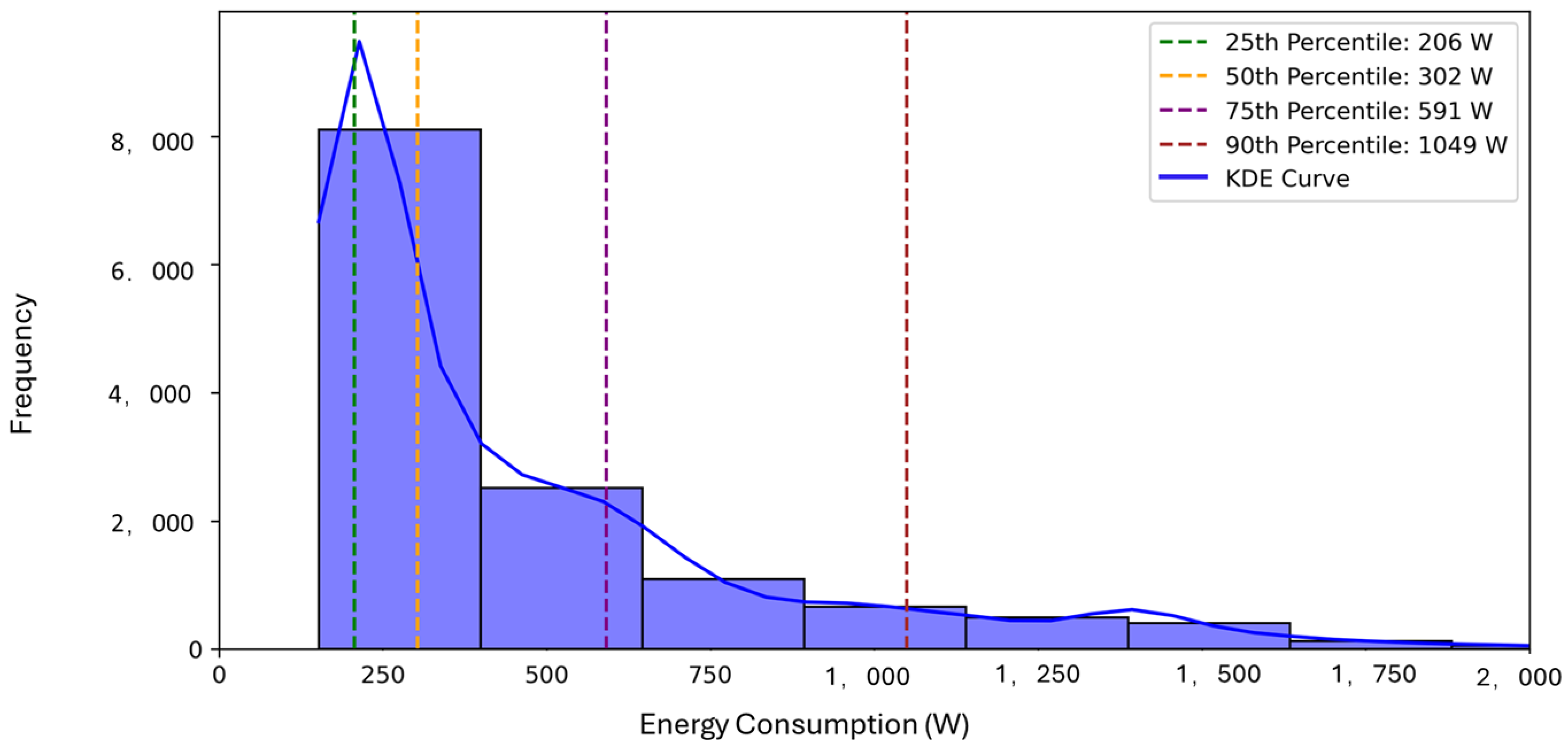Further statistics analysis for Building 01 are conducted, shown in Figure 1 and Figure 2. The blue bars in the histogram shows the frequency of different energy consumption levels. The histogram reveals a sharp peak at very low power consumption values (below 300 W), highlighting a dominant category of low-energy consumption periods. Beyond 300 W, the frequency of occurrences decreases significantly, suggesting that higher energy consumption levels are associated with different occupancy patterns or appliance usage behaviours. The Sturges method (red) and Freedman–Diaconis method (green) confirm the presence of a distinct peak in low power consumption ranges, which helps validate that 300 W falls at a natural cut-off between background energy use and higher consumption patterns. In Figure 2 the median value (50th percentile) is 302 W, indicating that half of the recorded energy usage values are below this level. This analysis confirms that 300 W serves as a threshold, guaranteeing that low-power background loads are not misclassified as occupancy.

A Random Forest Classifier was implemented to predict occupancy. Random Forest was chosen for occupancy classification due to its robustness in handling high-dimensional, nonlinear energy usage data. It provides strong predictive accuracy while maintaining computational efficiency, making it ideal for classifying occupancy states based on appliance usage patterns. Additionally, Random Forest offers built-in feature importance ranking, allowing for deeper insights into which appliances contribute most to occupancy prediction. This interpretability is particularly valuable for energy management applications, where understanding the key drivers of occupancy is critical for optimising energy efficiency. In the random forest classifier training, two feature sets were considered: one including aggregate energy consumption and another excluding it to evaluate the predictive power of appliance-level and contextual features alone. The model was evaluated using accuracy, precision, recall, and F1-score, and 5-fold cross-validation was applied to ensure robustness. In addition, the grid search method was applied to optimise the hyperparameters, like the number of trees, maximum depth, and minimum samples per leaf.

A feature ablation study was conducted to assess the contribution of individual appliances to occupancy prediction. Each appliance feature was removed one at a time, and the resulting drop in model accuracy was recorded. This analysis quantified the predictive power of specific appliances, identifying the appliances as key contributors to occupancy classification.

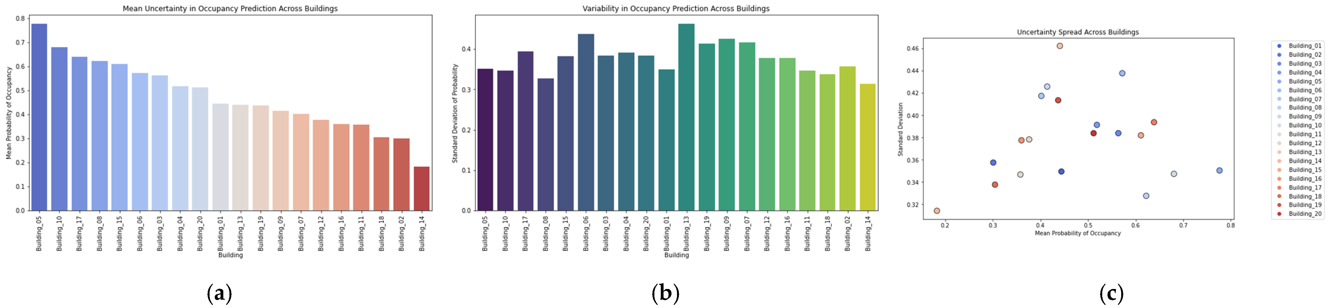
To further explore occupancy behaviour, K-means clustering and Gaussian Mixture Models (GMM) were applied to appliance-level energy consumption due to their effectiveness in segmenting energy consumption behaviours. K-means provides a fast and scalable method for identifying distinct occupancy groups based on energy usage, making it well-suited for high-dimensional appliance-level data. GMM complements K-means by allowing probabilistic membership assignments, which is particularly useful for households exhibiting transitional occupancy behaviours. The combination of these two methods ensures a comprehensive clustering approach that captures both rigid and flexible occupancy patterns. Hyperparameter selection for clustering models was guided by the Elbow Method and Silhouette Score analysis. The optimal number of clusters for K-means was determined by identifying the inflection point in the within-cluster sum of squares plot, where additional clusters provided marginal improvement. For GMM, the Bayesian Information Criterion (BIC) was optimised to balance model complexity and likelihood estimation, ensuring the best probabilistic representation of occupancy states.

The optimal number of clusters was determined using the Elbow Method, identifying distinct patterns in household energy usage. Clustering provided additional insights into occupancy-driven appliance usage behaviours. For GMM, the Bayesian Information Criterion (BIC) was optimised to balance model complexity and likelihood estimation, ensuring the best probabilistic representation of occupancy states.

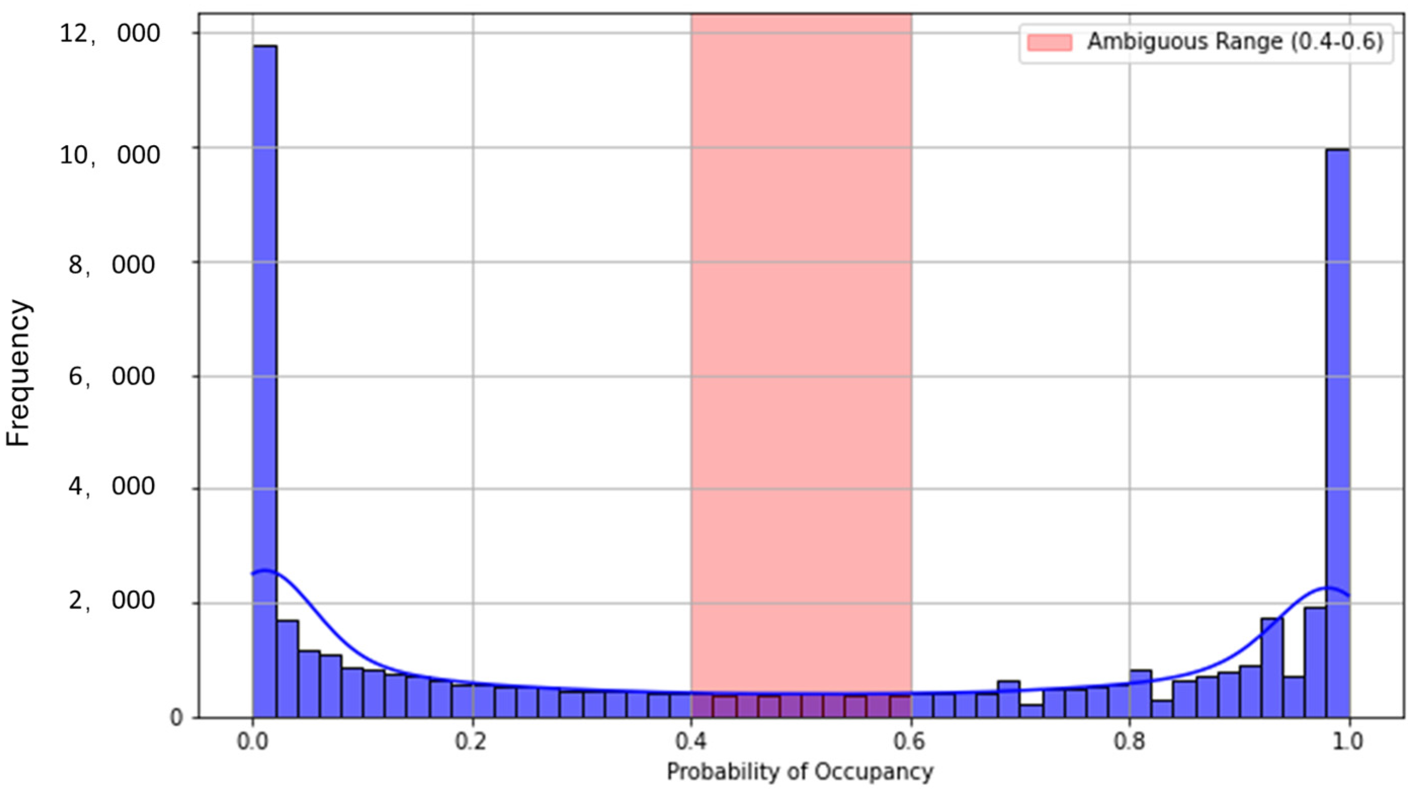
Probabilistic outputs from the classifier were analysed to quantify prediction uncertainty. Prediction probabilities between 0.4 and 0.6 were flagged as ambiguous cases, highlighting uncertain occupancy states. This uncertainty analysis informed further model refinements and decision boundary adjustments.

2.1.2. Single and Multi-Feature Time-Series Prediction

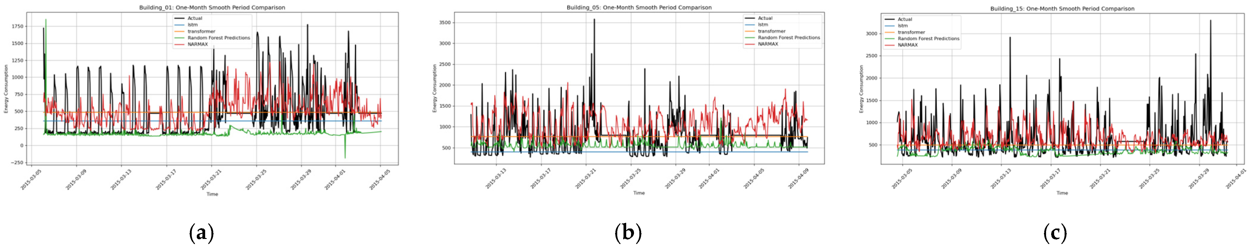
Time-series forecasting was conducted to predict aggregate energy consumption using both single and multiple features. The dataset was divided into 80% training and 20% testing, maintaining temporal continuity to prevent data leakage. Predictions were generated using various machine learning and deep learning models, ensuring a comprehensive evaluation of their performance in forecasting residential energy consumption. The selected models included LSTM, Transformer, NARMAX, SVM, ANN, XGBoost, and Random Forest. These models were chosen based on their ability to capture sequential dependencies, nonlinear relationships, and interpretability.

For single-feature prediction, models were trained using only time-related inputs, including hours of the day and day of the week, to predict aggregate energy consumption. The input data were transformed into a sequence format using a sliding window approach, where each training sample consisted of 24 consecutive hourly observations used to predict the next hour’s aggregate consumption.

A Long Short-Term Memory (LSTM) network was implemented for sequential modelling due to its proven effectiveness in capturing long-range dependencies in time-series data. The architecture consisted of two stacked LSTM layers, each with 50 units, followed by a dense output layer. Dropout regularisation with a rate of 0.2 was applied after each LSTM layer to prevent overfitting. The model was compiled using the Adam optimiser and trained with a Mean Squared Error (MSE) loss function. Hyperparameters such as the number of layers, units per layer, dropout rate, and learning rate were optimised using Bayesian optimisation with the Tree-structured Parzen Estimator (TPE), ensuring efficient tuning without excessive computational cost. Early stopping was implemented to monitor validation loss and prevent unnecessary training iterations. Predictions were de-normalised to restore the original scale of energy consumption.

A Transformer-based model was also employed as an alternative to LSTM, leveraging a self-attention mechanism to capture long-range dependencies in sequential data. Unlike recurrent networks, Transformers can dynamically assign different weights to different time steps using Multi-Head Self-Attention, improving model interpretability and efficiency. Positional encoding was introduced to provide the model with temporal awareness, and the final encoding of each time step was passed through a fully connected output layer to generate predictions. Similar to the LSTM model, the Transformer was trained using the Adam optimiser with an MSE loss function. Hyperparameters—including the number of attention heads, hidden dimensions, and feed-forward network size—were fine-tuned using Bayesian optimisation and early stopping to optimise generalisation.

NARMAX was introduced as an interpretable alternative to deep learning models. While LSTMs and Transformers provide high accuracy, they lack transparency in understanding the influence of input variables on predictions. NARMAX, in contrast, offers an explicit mathematical representation of system dynamics, making it valuable for energy managers seeking to understand causal dependencies in energy consumption. The general NARMAX model is defined as:

$$y\left(t\right)=F\left[y\left(t-1\right),\dots ,y\left(t-n_y\right),u\left(t\right),\dots ,u\left(t-n_u\right),e\left(t-1\right),\dots ,e(t-n_e)\right]$$

(1)

where $y$, $u$, and $e$ represent the system output, input and noise, $F$ is the general representation of some typical nonlinear model forms, like a polynomial model, neural network, and other kinds of nonlinear forms; $n_y$, $n_u$, and $n_e$ are the maximum time lags for the system output, input and noise. In the NARMAX modelling, the key procedure involves applying the Forward Regression Orthogonal Least Square (FROLS) algorithm to detect the model structure and estimate the parameters. This approach ensures that only the most significant variables are retained, enhancing interpretability while maintaining predictive power. Unlike deep learning models, which often act as black boxes, NARMAX allows energy managers to identify which factors most influence consumption patterns and develop targeted efficiency strategies based on these insights.

Beyond its interpretability, NARMAX supports predictive control applications in energy management. By analysing its explicit equations, energy managers can optimise HVAC systems, lighting, and appliance scheduling based on forecasted energy demands. Moreover, regulatory compliance and reporting benefit from NARMAX’s transparency, as the model provides a structured way to demonstrate how different variables impact energy consumption. This capability is particularly valuable in settings where decision-makers require explainable and audit-friendly models for policy enforcement and sustainability reporting.

The model complexity was controlled using the Akaike Information Criterion (AIC) and Bayesian Information Criterion (BIC), ensuring an optimal balance between interpretability and predictive power.

To improve forecasting accuracy, multiple contextual features—including temperature, humidity, brightness, and climate conditions—were incorporated alongside time-series data. These additional inputs allowed models to capture environmental influences on energy consumption. Data preprocessing involved merging external feature datasets with aggregate energy consumption data based on timestamps. Mean imputation was applied to handle missing values, and all features were normalised to ensure stable training. The sliding window method was extended to include both past energy consumption and contextual variables as input sequences.

A deep learning-based multi-feature LSTM model was developed to process these inputs. The architecture followed a similar structure to the single-feature LSTM but with an expanded input space to accommodate external variables. The network consisted of two LSTM layers with 50 units each, followed by a dense output layer. The ReLU activation function was used for non-linear transformations, and dropout layers (rate = 0.2) were included to prevent overfitting. The training was conducted using the Adam optimiser, and the MSE loss function was minimised over 50 epochs with early stopping. Hyperparameter tuning, including batch size and learning rate adjustments, was conducted using a combination of grid search and Bayesian optimisation.

A Transformer model was also employed for multi-feature prediction. The input feature set was passed through multiple self-attention layers, allowing the model to adjust the importance of different inputs over time dynamically. The final encoding of each time step was used to generate predictions, similar to the single-feature Transformer setup. Model hyperparameters—including the number of attention heads and feed-forward network dimensions—were tuned for optimal performance.

To benchmark forecasting performance across different modelling approaches, additional machine learning models—including Support Vector Machines (SVM), Artificial Neural Networks (ANN), Extreme Gradient Boosting (XGBoost), and Random Forest—were evaluated. These models were chosen based on their ability to capture nonlinear relationships and generalise well across diverse datasets. Each model was trained on the same dataset split and evaluated using Root Mean Squared Error (RMSE) and Coefficient of Variation (CV) to assess prediction accuracy. Hyperparameter tuning for SVM involved optimising the kernel function (RBF vs. polynomial) and regularisation parameter (C) using grid search. For ANN, the number of hidden layers, activation functions, and dropout rates were fine-tuned through random search and cross-validation. The XGBoost model was optimised using learning rate tuning, tree depth adjustments, and feature importance analysis. Random Forest hyperparameters, including the number of estimators and tree depth, were selected based on grid search and k-fold cross-validation.

Each model was selected based on its suitability for time-series forecasting and its ability to capture different characteristics of energy consumption. LSTM and Transformer models were chosen for their ability to learn long-range dependencies, NARMAX for its interpretability, and ensemble models like Random Forest and XGBoost for their robustness in feature-driven forecasting. A structured hyperparameter tuning process, incorporating grid search, random search, Bayesian optimisation, and cross-validation, was applied across all models to ensure optimal predictive performance in diverse energy datasets.

2.2. Dataset Description

The proposed framework is applied to the REFIT Smart Home dataset, a comprehensive resource for residential energy consumption research collected during the REFIT project (2013–2015). This dataset includes high-resolution energy usage data from 20 UK households retrofitted with smart home technologies, making it ideal for addressing the complexities of building energy management. The dataset’s granularity and contextual richness provide a strong foundation for appliance-level energy prediction, temporal analysis, and archetype-based modelling.

The dataset includes electrical load data, offering cleaned measurements of energy consumption in Watts at both aggregate and appliance levels. These data are sampled at 8-second intervals, enabling a detailed examination of short-term energy dynamics. Appliance-level measurements cover a range of household devices, such as refrigerators, washing machines, and microwaves, allowing granular analysis of specific energy usage patterns. Aggregate-level data, on the other hand, capture the total energy consumption of each household. In addition, the dataset features building survey data that capture the structural and operational characteristics of each household. These surveys include information on building type (e.g., detached, semi-detached, or terraced), size (e.g., number of rooms and floors), appliance inventory, and occupancy details. Another key component of the dataset is the climate data collected from a nearby weather station. These data include variables such as temperature, humidity, brightness, and wind speed, all of which significantly influence residential energy consumption. For instance, temperature and humidity are critical for modelling seasonal energy demands related to heating or cooling.

3. Results

3.1. Occupancy Pattern Analysis

This section presents the results of occupancy classification, feature importance analysis, clustering, and uncertainty estimation, focusing solely on appliance-level and contextual features without using aggregate energy consumption as an input.

The information for the 20 buildings is summarised in

Table 1. Summary of the building information.

House ID	Users	Construction Year	Type	Size	Occupancy	Energy Consumption Pattern
1	2	1975–1980	Detached	4 beds	Frequent	High-Energy
2	4	-	Semi-detached	3 beds	Variable	Moderate-Energy
3	2	1988	Detached	3 beds	Variable	Moderate-Energy
4	2	1850–1899	Detached	4 beds	Variable	Moderate-Energy
5	4	1878	Mid-terrace	4 beds	Irregular	Low-Energy
6	2	2005	Detached	4 beds	Irregular	Low-Energy
7	4	1965–1974	Detached	3 beds	Frequent	High-Energy
8	2	1966	Detached	2 beds	Variable	Moderate-Energy
9	2	1919–1944	Detached	3 beds	Frequent	High-Energy
10	4	1919–1944	Detached	3 beds	Irregular	Low-Energy
11	1	1945–1964	Detached	3 beds	Irregular	Low-Energy
12	3	1991–1995	Detached	3 beds	Irregular	Low-Energy
13	4	post 2002	Detached	4 beds	Irregular	Low-Energy
14	1	1965–1974	Semi-detached	3 beds	Irregular	Low-Energy
15	6	1981–1990	Detached	5 beds	Irregular	Low-Energy
16	3	mid 60s	Detached	3 beds	Irregular	Low-Energy
17	2	1965–1974	Detached	3 beds	Irregular	Low-Energy
18	4	1945–1964	Semi-detached	3 beds	Irregular	Low-Energy
19	2	1965–1974	Detached	3 beds	Irregular	Low-Energy
20	4	1981–1990	Detached	3 beds	Irregular	Low-Energy

. This table provides a structured summary of 20 buildings, detailing their occupancy, year of construction, type, size, and corresponding energy consumption patterns. The analysis classifies the buildings into three distinct energy usage profiles, based on occupancy patterns (frequent, variable, and irregular). Occupancy significantly influences energy usage—consistent occupancy usually results in increased consumption, while sporadic occupancy corresponds to lower consumption levels. Detached houses with over four residents typically have greater energy demands, whereas smaller homes with fewer occupants demonstrate reduced usage. Generally, older structures (constructed before 1965) tend to display lower energy consumption, possibly attributed to less appliance usage or more energy-efficient habits.

Three buildings are selected to show the results of occupancy pattern analysis to cover different types of buildings.

• Building 1: A detached residential structure, constructed between 1975 and 1980, accommodating two individuals and is equipped with 35 appliances distributed across four bedrooms.
• Building 5: This mid-terrace dwelling, built in 1878, houses four occupants, has 44 appliances, and includes four bedrooms.
• Building 14: This semi-detached building, constructed between 1965 and 1974, is occupied by a single individual. It is furnished with 19 appliances and three bedrooms.

3.1.1. Clustering Analysis of Occupancy Patterns

The Elbow Method determined that the optimal number of clusters was three, reflecting variations in household occupancy and appliance usage patterns. The clustering results for Building 01 are visualised as the example in Figure 3.

In the result for the elbow method, K = 3 was selected for the number of clusters, marking the transition where increasing the number of clusters no longer significantly reduces inertia. Figure 3b,c present the clustering results for pairing normalised fridge-freezer usage and washing machine usage, where higher values on either axis indicate higher appliance usage. Data points clustered close to the origin with low x and y values signify low usage behaviour. Points that are outliers with high x or y values indicate high appliance usage. Data points with moderate values for one or both appliances reflect mid-usage behaviour. Both two clustering methods agree that the majority of the data belong to Cluster 2. K-Means creates a hard boundary for these points, excluding all outliers in the process, while GMM reflects the uncertainty in this dense region, with some points probabilistically assigned to Cluster 1. High fridge-freezer usage (e.g., $x>10$) is consistently assigned to Cluster 0, similar to washing machines. However, GMM softens the assignments by assigning smaller probabilities to secondary clusters.

To better compare the clustering results for 20 buildings, meta-clustering is conducted to group the buildings with similar performance. From each building’s clustering, the cluster proportions and silhouette score are selected to group the buildings; results are shown in

Table 2. Meta-clustering results for 20 buildings.

Building ID	Cluster 1 Proportion	Cluster 2 Proportion	Cluster 3 Proportion	Avg. Silhouette	Meta-Cluster
01	0.37	0.28	0.35	0.58	2
02	0.40	0.39	0.21	0.56	1
03	0.38	0.37	0.25	0.60	1
04	0.36	0.35	0.28	0.59	1
05	0.35	0.33	0.32	0.58	0
06	0.35	0.35	0.30	0.56	0
07	0.37	0.29	0.34	0.57	2
08	0.37	0.37	0.27	0.58	1
09	0.35	0.29	0.37	0.56	2
10	0.35	0.32	0.33	0.58	0
11	0.35	0.33	0.31	0.59	0
12	0.34	0.31	0.35	0.58	0
13	0.32	0.38	0.30	0.60	0
14	0.33	0.32	0.35	0.58	0
15	0.32	0.36	0.32	0.60	0
16	0.32	0.34	0.34	0.58	0
17	0.33	0.34	0.33	0.59	0
18	0.32	0.34	0.34	0.58	0
19	0.34	0.32	0.34	0.58	0
20	0.32	0.33	0.36	0.60	0

. The meta-clustering revealed three distinct building groups based on clustering patterns: high variability, moderate variability, and low variability.

The silhouette scores range between 0.56 and 0.60, which is a relatively small range. This suggests that no meta-cluster has significantly stronger cohesion/separation from the others. Buildings in Meta-cluster 0 exhibit similar proportions of all three clusters, indicating that there is no single dominant cluster. Buildings categorised in Meta-cluster 1 do not reveal a clear dominant cluster, suggesting that these buildings may experience significant variation in appliance usage over time. In contrast, buildings within Meta-cluster 2 display the dominance of one cluster, implying that most of their data points belong to a single cluster or that their silhouette scores are relatively lower (closer to 0.56), which indicates some overlap between clusters.

Representative meta-clustering grouping results for Buildings 07, 08, and 17 illustrate these groups, as shown in Figure 4. Building 17, which represents Meta-Cluster 0, demonstrates more stable cluster patterns. Building 08, located in Meta-Cluster 1, indicates that appliance usage fluctuates, making clustering less effective. Building 07, belonging to Meta-Cluster 2, suggests very dominant energy usage behaviours.

The household energy profiles can be characterised into three clusters as follows:

Cluster 1 (High-Energy, Frequent Occupancy Households): Homes with consistent occupancy and high appliance usage throughout the day, indicating families with multiple occupants or individuals working from home.

Cluster 2 (Moderate-Energy, Variable Occupancy Households): Homes with moderate appliance activity, where occupancy fluctuates across different hours and days.

Cluster 3 (Low-Energy, Irregular Occupancy Households): Homes with sporadic appliance usage, suggesting single-occupant households or part-time occupancy.

Based on the meta-clustering results and the observed clustering visualisations, three appliance-usage-based household categories (Cluster 1, Cluster 2, Cluster 3) aligned with the meta-cluster groups (0, 1, 2), summarised in

Table 3. Mapping household energy profiles to meta-clusters.

Meta-Cluster	Household Type	Buildings Assigned
Meta-Cluster 0	Low-Energy, Irregular Occupancy (Cluster 3)	01, 07, 09
Meta-Cluster 1	Moderate-Energy, Variable Occupancy (Cluster 2)	02, 03, 04, 08
Meta-Cluster 2	High-Energy, Frequent Occupancy (Cluster 1)	05, 06, 10–20

.

3.1.2. Occupancy Classification Performance

The Random Forest classifier was trained and tested using appliance-level features from 20 buildings. The model was evaluated using accuracy, precision, recall, and F1-score, with results summarised in

Table 4. Occupancy classification performance across 20 buildings.

Building ID	Accuracy	Precision	Recall	F1-Score
Building 01	0.81	0.81	0.81	0.80
Building 05	0.95	0.95	0.95	0.95
Building 14	0.92	0.92	0.92	0.92
Mean	0.89	0.89	0.89	0.89
Stand Deviation	0.06	0.06	0.06	0.06

.

Overall, the classifier achieved a mean accuracy of 89%, demonstrating strong predictive performance across different buildings using only appliance-level data. Buildings with more consistent appliance usage patterns (e.g., regular washing machine cycles) exhibited higher classification accuracy, while buildings with irregular energy usage behaviours showed slightly lower performance.

A confusion matrix for three representative buildings (high-, medium-, and low-energy users) is presented in Figure 5, illustrating classification performance in detail. False positives primarily occurred during low-energy appliance activity periods, where minor fluctuations in consumption led to misclassifications.

3.1.3. Feature Importance and Drop-In Accuracy Analysis

To assess the contribution of each appliance to occupancy classification, a feature importance analysis was conducted using the trained Random Forest model. The ranking of appliance features is presented in Figure 6, where higher values indicate stronger predictive power.

For example, the washing machine, dishwasher and fridge-freezer were identified as the most influential features in Building 01. This aligns with expectations, as these appliances typically operate during occupied periods and exhibit distinct usage patterns compared to other devices.

A drop-in accuracy analysis was performed to further validate the importance of individual appliances. Each appliance feature was removed sequentially, and the corresponding decrease in classification accuracy was recorded. For each building, the mean drop in accuracy across all key features is computed, providing a single representative value for how sensitive the building’s classification is to the removal of key features. After ranking all buildings by the mean drop in accuracy, three buildings are selected to represent high, low and balanced performance. Figure 7 illustrates the representative buildings, where Building 01 has the highest mean drop across features, highlighting the prediction that Building 01 relies heavily on specific features. Building 11 has the lowest mean drop across features, showing the robustness of the classification model, as it does not depend heavily on any one feature. The results for Building 11 indicate that the model performs consistently across all features.

3.1.4. Uncertainty Analysis in Occupancy Classification

Occupancy classification was performed using the Random Forest method. To quantify the confidence of the occupancy classifier, the model’s predicted probabilities were analysed. A probability close to 0 or 1 indicates high confidence, while a probability near 0.5 suggests the model is uncertain. The uncertain classifications are defined as those where the predicted probability falls within a range of 0.4 to 0.6. This range represents cases where the model struggles to confidently assign an instance to either “occupied” or “not occupied”.

Figure 8 presents a histogram of predicted probabilities of Building 01. The red-shaded region (0.4 to 0.6) marks the ambiguous predictions, where the classifier struggles the most. The result indicates that the majority of predictions are clustered near 0 and 1, indicating that the model is confident in classifying most time instances as either occupied (1) or unoccupied (0). This suggests that Building 01 has clear occupancy patterns, where usage aligns strongly with either fully occupied or unoccupied states. A moderate proportion of predictions (~15%) fall within the ambiguous range. The probabilities between 0.1 and 0.4 and 0.6 to 0.9 suggest that there are periods of partial occupancy uncertainty, where activity fluctuates but does not reach a confident classification. This might correspond to sporadic appliance use or inconsistent behavioural patterns in the building.

Similarly, the same uncertainty analysis is conducted for the remaining buildings, and the aggregate analysis is summarised in Figure 9. Most predictions are concentrated near 0 (unoccupied) and 1 (occupied). This suggests that the model is generally confident in classifying occupancy states. A small but notable number of predictions fall into the red-shaded range, where the model is uncertain about occupancy. The blue line is the KDE (Kernel Density Estimate) line overlaying a smooth density estimate of probabilities, which confirms sharp peaks at 0 and 1 and a relatively flat region in the ambiguous range. The model is highly confident for most time periods, but uncertainty exists for about 15% of cases (as seen in the ambiguous range). Buildings with consistent energy patterns (e.g., routine appliance usage) have fewer ambiguous predictions.

To determine which buildings contribute the most to uncertainty, the mean probability of occupancy and standard deviation (std) are focused. A mean occupancy probability near 0.5 suggests more uncertain predictions. Buildings with means between 0.4 and 0.6 are more ambiguous. A high standard deviation indicates greater variability in occupancy predictions, implying fluctuating occupancy behaviour. The visualisations are displayed in Figure 10. Buildings 05, 06, 08, 10, and 17 have higher mean uncertainty and standard deviation, which could be due to inconsistent occupancy patterns, irregular appliance usage, or external environmental factors affecting predictions. Buildings 02, 14, 16, and 18, with low uncertainty, have more predictable occupancy, making it easier for the model to classify with confidence.

This uncertainty analysis reinforces the need for probabilistic energy modelling to accommodate ambiguous cases and improve decision-making in smart energy management.

3.2. Time-Series Prediction of Energy Consumption

This section evaluates the performance of single-feature and multiple-feature energy consumption forecasting models across all 20 buildings. The models were assessed using Root Mean Squared Error (RMSE) and Coefficient of Variation (CV) to quantify prediction accuracy.

3.2.1. Single-Feature Prediction Results

Aggregate energy consumption was predicted using only time-based features. LSTM and Transformer models were trained using 24 h sequences to forecast the next-hour energy consumption. The RMSE and CV values for selected buildings are summarised in

Table 5. RMSE of time-series prediction models (single-feature input).

Building ID	RMSE
	LSTM	Transformer	SVM	NARMAX	Random Forest	XGBoost
Building 01	280.840	289.257	289.737	253.615	445.988	436.339
Building 02	580.692	596.388	606.542	531.620	712.300	661.913
Building 03	488.530	530.565	534.036	485.911	786.650	548.777
Building 04	151.498	153.742	161.285	148.627	185.669	166.358
Building 05	337.691	364.870	361.556	343.663	535.614	466.773
Building 06	183.039	179.676	179.492	159.478	212.097	204.324
Building 07	390.583	415.331	404.487	396.713	465.600	444.108
Building 08	628.899	598.401	683.821	470.045	676.212	666.005
Building 09	486.542	494.429	489.253	466.484	598.420	559.414
Building 10	483.438	448.388	454.781	433.740	531.223	509.059
Building 11	407.975	411.626	487.744	303.801	434.738	409.987
Building 12	266.650	265.691	272.404	259.388	305.206	270.909
Building 13	595.766	596.717	614.510	487.713	658.976	644.520
Building 14	155.099	155.691	155.003	157.950	186.901	178.885
Building 15	280.772	259.180	274.446	243.129	396.730	366.786
Building 16	433.475	374.204	376.416	361.985	960.573	762.215
Building 17	280.092	287.384	287.588	266.227	321.525	288.658
Building 18	151.933	152.254	152.769	148.234	178.589	157.439
Building 19	198.733	214.328	208.175	194.196	251.752	233.554
Building 20	604.016	377.738	660.338	304.357	684.680	653.578

and

Table 6. CV of time-series prediction models (single-feature input).

Building ID	CV
	LSTM	Transformer	SVM	NARMAX	Random Forest	XGBoost
Building 01	67.696	69.725	69.841	61.134	107.505	105.179
Building 02	108.930	111.874	113.779	99.725	133.618	124.166
Building 03	73.905	80.264	80.789	73.509	119.004	83.019
Building 04	42.571	43.202	45.322	41.765	52.173	46.747
Building 05	47.303	51.111	50.646	48.140	75.028	65.385
Building 06	37.256	36.572	36.534	32.461	43.171	41.589
Building 07	76.404	81.245	79.124	77.603	91.079	86.874
Building 08	85.996	81.826	93.507	64.275	92.466	91.070
Building 09	89.105	90.549	89.601	85.432	109.594	102.451
Building 10	77.847	72.203	73.233	69.845	85.542	81.973
Building 11	68.536	69.149	81.936	51.036	73.032	68.874
Building 12	74.599	74.331	76.209	72.567	85.386	75.791
Building 13	92.152	92.299	95.051	75.439	101.929	99.693
Building 14	70.773	71.043	70.729	72.074	85.285	81.627
Building 15	70.333	64.925	68.748	60.904	99.381	91.880
Building 16	109.159	94.234	94.791	91.156	241.895	191.944
Building 17	61.091	62.681	62.726	58.067	70.128	62.959
Building 18	54.679	54.795	54.980	53.348	64.273	56.661
Building 19	54.375	58.642	56.958	53.133	68.881	63.902
Building 20	65.778	73.367	71.911	33.145	74.562	71.175

.

Across 20 buildings, LSTM, Transformer, and NARMAX generally stayed within 10–15% of each other in RMSE. In more predictable households, NARMAX outperformed others by up to 12%, whereas Transformer led by roughly 8–10% in irregular-demand settings. Meanwhile, SVM lagged 10–20% behind top performers, and Random Forest or XGBoost often trailed by 20–25%, indicating challenges with purely time-based inputs. In certain high-consumption buildings, LSTM registered the lowest errors, while NARMAX excelled with moderate loads. Transformers also showed reliable accuracy but could be sensitive to hyperparameter choices. Collectively, these outcomes highlight the marked impact of occupant-driven variability on time-only forecasting.

In Figure 11a, Building 01 demonstrates a relatively stable energy consumption pattern, with LSTM and Transformer models closely tracking actual consumption. Both models capture the long-term trend effectively, with minor deviations. NARMAX, while maintaining interpretability, consistently underestimates energy usage, resulting in a lower predicted range. Random Forest Predictions introduce substantial fluctuations, with frequent spikes that deviate significantly from actual consumption, highlighting its difficulty in adapting to stable energy demand. However, it is important to note that this figure represents only a small portion of the entire testing period, and the overall performance of NARMAX across the full dataset is stronger than it appears in this subset.

Figure 11b presents the results for Building 05, where LSTM and Transformer models continue to show strong alignment with actual consumption trends. Both models provide smooth and accurate predictions, reinforcing their ability to generalise across different households. NARMAX offers reasonable performance but appears to struggle in capturing certain variations within this selected period. Random Forest Predictions exhibit erratic behaviour with high variance, failing to align well with the stable consumption pattern observed in this building. While these observations highlight the effectiveness of deep learning models within this timeframe, across the full testing period, NARMAX demonstrates superior overall accuracy in more predictable households.

Figure 11c illustrates the performance for Building 15, where LSTM and Transformer maintain their accuracy advantage, effectively modelling the stable consumption period. NARMAX performs slightly worse compared to the previous cases, showing more variation in its predictions, occasionally diverging from actual consumption values. Random Forest Predictions remain inconsistent, introducing substantial noise and deviating from actual consumption with frequent spikes, making it the least reliable model for this scenario. Despite these short-term observations, the broader dataset analysis indicates that NARMAX achieves better overall performance than the deep learning models in structured energy demand scenarios.

Figure 11 provide insight into how different models perform over a selected stable period, but they do not fully represent model performance across the entire testing set. In the full dataset, NARMAX outperforms LSTM and Transformer in many buildings, particularly where energy consumption patterns are more predictable. Overall, the figures illustrate that LSTM and Transformer models effectively capture stable consumption trends within the selected time periods, closely following actual energy usage with minimal deviation. However, these figures only represent a subset of the testing period. In the complete testing set, NARMAX demonstrates superior overall performance, as reflected in the RMSE and CV results, particularly in more predictable households. While NARMAX appears to underestimate fluctuations in these selected periods, its structured regression approach allows it to generalise better across the full dataset. Random Forest Predictions continue to exhibit pronounced fluctuations, making them less reliable for modelling smooth energy consumption patterns. These results reinforce that while deep learning models excel at handling short-term variations, NARMAX remains a strong contender over the entire dataset due to its robustness in structured energy demand scenarios.

3.2.2. Multiple-Feature Prediction Results

To assess the impact of contextual variables on energy prediction, models were trained using temperature, humidity, brightness, and other external features. The results in

Table 7. RMSE of time-series prediction models (multi-feature input).

Building ID	RMSE
	LSTM	Transformer	SVM	NARMAX	Random Forest	XGBoost
Building 01	280.840	289.257	289.737	291.301	445.988	436.339
Building 02	580.631	596.484	606.635	583.851	712.177	661.860
Building 03	488.582	530.597	534.059	550.867	786.746	548.852
Building 04	151.511	153.749	161.304	181.248	185.653	166.375
Building 05	337.728	364.929	361.615	357.436	535.632	466.632
Building 06	180.250	176.850	176.416	209.808	209.576	201.829
Building 07	390.648	415.398	404.556	368.684	465.676	444.181
Building 08	629.013	598.499	683.942	624.113	676.337	666.128
Building 09	486.387	494.489	489.304	423.288	597.332	559.192
Building 10	483.523	448.468	454.861	465.983	531.307	509.139
Building 11	407.715	411.724	487.586	412.959	434.688	409.891
Building 12	266.650	265.691	272.404	222.830	305.206	270.909
Building 13	595.707	596.655	614.104	586.351	659.072	644.649
Building 14	155.283	155.824	155.134	140.126	187.147	179.140
Building 15	280.611	259.519	274.175	237.710	396.609	366.929
Building 16	434.700	376.583	378.725	456.941	966.143	766.608
Building 17	280.092	287.384	287.588	202.443	321.525	288.658
Building 18	151.948	152.125	152.673	189.623	178.708	157.475
Building 19	199.525	214.829	209.102	110.259	250.876	233.607
Building 20	604.016	377.771	660.338	604.357	684.680	653.578

and

Table 8. CV of time-series prediction models (multi-feature input).

Building ID	CV
	LSTM	Transformer	SVM	NARMAX	Random Forest	XGBoost
Building 01	67.696	69.725	69.841	69.427	107.505	105.179
Building 02	108.903	111.876	113.780	73.019	133.575	124.138
Building 03	73.927	80.284	80.808	74.744	119.042	83.047
Building 04	42.571	43.200	45.323	51.123	52.165	46.748
Building 05	47.305	51.115	50.651	46.093	75.025	65.360
Building 06	36.737	36.044	35.955	35.904	42.714	41.135
Building 07	76.396	81.236	79.116	75.769	91.068	86.865
Building 08	85.993	81.821	93.502	84.597	92.462	91.067
Building 09	89.076	90.559	89.610	89.461	109.394	102.409
Building 10	77.860	72.215	73.245	71.344	85.555	81.985
Building 11	68.536	69.210	81.962	69.657	73.070	68.902
Building 12	74.599	74.331	76.209	75.292	85.386	75.791
Building 13	92.214	92.361	95.062	93.205	102.023	99.790
Building 14	70.895	71.142	70.827	70.630	85.443	81.787
Building 15	69.873	64.621	68.270	66.991	98.757	91.366
Building 16	109.504	94.864	95.403	105.488	243.378	193.113
Building 17	61.091	62.681	62.726	61.588	70.128	62.959
Building 18	54.633	54.696	54.893	52.133	64.254	56.620
Building 19	54.419	58.594	57.031	56.896	68.425	63.715
Building 20	65.778	73.370	71.911	73.145	74.562	71.175

compare forecasting performance with and without additional features.

Including temperature, humidity, or occupancy proxies improved LSTM and Transformer accuracy by up to 15%, particularly in weather-sensitive households, while SVM exhibited gains of approximately 10%. NARMAX’s RMSE generally showed stable or improved performance, with reductions of 5–8% in many cases. However, in certain high-variance settings, RMSE remained relatively unchanged or increased slightly, likely due to inconsistencies in external variable relevance across different buildings rather than overfitting. The refined feature selection using AIC/BIC and cross-validation effectively mitigated previous overfitting concerns.

Random Forest and XGBoost achieved moderate improvements of 5–12%, reinforcing the benefit of ensemble models in capturing nonlinear dependencies. In homes with erratic occupant schedules, deep learning methods maintained a strong advantage, reducing errors by more than 20% due to their ability to handle complex feature interactions. Conversely, in cases where environmental data had weak correlations with peak consumption, all models exhibited only marginal improvements. These results emphasise the importance of context-specific feature selection in optimising predictive performance while maintaining model stability.

In Figure 12a, Building 01’s energy consumption is modelled with multi-feature inputs during the selected stable period from 5 March 2015 to 5 April 2015. The LSTM and Transformer models show strong predictive performance, aligning closely with actual consumption trends, particularly during moderate consumption fluctuations. The inclusion of additional features allows these models to capture energy consumption dynamics more effectively. The NARMAX model exhibits improved tracking of overall patterns compared to traditional methods, but still demonstrates sensitivity to overfitting, particularly in certain peak consumption periods. The Random Forest model continues to struggle with capturing variability, often underestimating actual consumption.

Figure 12b illustrates the prediction performance for Building 05 from 13 March 2015, to 9 April 2015. During this period, the LSTM and Transformer models maintain superior accuracy, capturing both short-term fluctuations and underlying trends more effectively than other models. The NARMAX model, though benefiting from multi-feature inputs, still exhibits periodic underestimation and struggles to fully adapt to abrupt spikes in energy consumption. The Random Forest model remains stable but lacks responsiveness to sudden shifts, leading to consistent deviations from actual values. The presence of multi-feature data has reduced prediction variance across all models, highlighting the benefits of contextual input in improving forecasting accuracy.

Figure 12c presents the results for Building 15 from 5 March 2015, to 1 April 2015, where Transformer and LSTM models continue to demonstrate their advantages in dynamic energy prediction. The Transformer model slightly outperforms LSTM during peak consumption periods, reinforcing its ability to process sequential dependencies effectively. NARMAX displays mixed performance, accurately capturing baseline trends but showing inconsistencies in highly variable consumption intervals. The Random Forest model remains less responsive to fluctuations, reinforcing its limitations in time-series forecasting despite the incorporation of multi-feature data.

Figure 12 highlight how multi-feature models significantly enhance predictive accuracy compared to single-feature approaches. LSTM and Transformer models consistently exhibit strong performance across different buildings and periods, effectively leveraging contextual variables to adjust predictions based on external factors. The NARMAX model, while offering interpretability, shows susceptibility to overfitting in some cases. Traditional machine learning models, particularly Random Forest, maintain stability but are limited in capturing rapid energy consumption changes. While the time period displayed in these figures represents a stable subset of the overall testing period, results from the full dataset confirm that NARMAX outperforms other models across the entire evaluation period, as indicated by RMSE values in the comprehensive performance tables. This underscores the importance of both time-series adaptability and feature selection in optimising building energy consumption forecasting. It is important to note that these figures represent only a selected portion of the testing period, and overall performance across the entire dataset suggests that NARMAX achieves competitive accuracy in many cases, as indicated by the RMSE and CV values in the results tables.

4. Discussion

The findings from this study demonstrate that combining occupancy pattern analysis with advanced time-series prediction can significantly enhance building energy management and forecasting. By employing Random Forest classification and clustering (K-means, GMM, and meta-clustering), it revealed nuanced household energy usage behaviours and provided a basis for more targeted management strategies. These insights align with the broader goals of the Sparse, Interpretable, and Transparent (SIT) framework, where model parsimony, result explainability, and prediction clarity are key.

From an occupancy perspective, the clustering outcomes indicate three main groups of appliance usage intensity (low, moderate, and high), each associated with distinct occupant behaviours. In particular, meta-clustering served as a scalable means to group and compare multiple buildings, highlighting shared consumption patterns across different households. These insights confirm that occupant behaviour plays a central role in driving load variability—an observation supported by earlier research on occupancy-driven energy demand. Moreover, the Random Forest classifier underscored the importance of certain appliances, notably the fridge-freezer and washing machine, as reliable indicators of occupancy. The drop-in accuracy analysis further reinforced how specific appliances strongly correlate with occupant presence. Such interpretability provides practical value: building managers can focus on the most impactful end-users to develop targeted interventions.

Uncertainty analysis of occupancy classification demonstrated that a modest but non-negligible portion of time periods remain ambiguously predicted (i.e., predicted probabilities near 0.5). These uncertain predictions mostly occurred in two contexts: (1) during overnight or early-morning hours when aggregate consumption is minimal and (2) in households exhibiting highly irregular or sporadic appliance usage. Probabilistic approaches to occupancy detection, therefore, may improve real-time decision-making in building energy systems, particularly when occupant presence critically influences HVAC or demand response operations.

In time-series forecasting, the results showed that LSTM and Transformer architectures generally traditional machine learning models (Random Forest, SVM, XGBoost) when only time-of-day or day-of-week inputs were used. This performance gap widened in buildings with pronounced load fluctuations or highly dynamic occupant schedules, consistent with previous literature on deep learning’s ability to capture nonlinear temporal dependencies [25,26]. Notably, integrating contextual features such as temperature and humidity led to further improvements in predictive accuracy, often reducing errors by 10–20% in weather-sensitive buildings. However, these performance gains varied across households—some experienced marginal benefits if weather factors were weak predictors of peak loads, indicating that occupant behaviour often remains the more dominant influence on consumption patterns.

The NARMAX-based SIT approach demonstrated a nuanced performance, balancing interpretability and predictive capability. Under stable or moderately variable conditions, its structured regression framework yielded accuracy comparable to deep learning models while offering clear insights into the relationships between input variables and energy consumption. This interpretability is particularly valuable for energy managers seeking to develop data-driven operational strategies.

However, in highly volatile settings, NARMAX exhibited sensitivity to the inclusion of multiple external features, increasing the risk of overfitting. This highlights the need for careful model selection and tuning to accommodate the inherent variability in building energy data. Addressing this challenge requires further exploration of regularisation techniques and feature selection strategies to enhance NARMAX’s robustness in dynamic environments.

Despite these limitations, the ability of NARMAX to provide explicit mathematical formulations makes it a strong candidate for applications where decision-making transparency is essential. By identifying key energy drivers and enabling predictive control measures, NARMAX supports energy efficiency optimisation, proactive demand-side management, and compliance with regulatory frameworks. Future work should focus on integrating uncertainty quantification techniques to further improve the generalizability of NARMAX-based approaches in real-world energy management scenarios.

While the dataset used in this study was collected between 2013 and 2015, the fundamental energy consumption patterns—such as occupancy-driven demand fluctuations, seasonal variations, and the impact of external factors like temperature—remain structurally consistent over time. However, it is acknowledged that advancements in smart home technologies, energy efficiency policies, and evolving occupancy behaviours may introduce deviations in more recent or future datasets.

To address this, our methodology is designed to be adaptable to newer datasets, as the models used can be retrained with updated data while preserving their interpretability. Future work could involve validating these findings using more recent energy consumption datasets to assess whether the observed patterns hold over time or if additional model adjustments are required. This would further strengthen the applicability of our approach to evolving energy consumption trends.

5. Conclusions

This paper presented a hybrid machine-learning framework aimed at improving building energy forecasting through occupancy pattern analysis and time-series modelling. The results demonstrate that identifying key occupancy-driven appliance features and clustering usage behaviours offer valuable insights into the temporal and contextual variability of residential loads. Furthermore, combining these occupancy findings with advanced forecasting models (e.g., LSTM and Transformer networks) significantly enhances predictive accuracy, particularly when external variables such as weather are incorporated.

The interpretability of the proposed approach also proved advantageous. Random Forest classifications, supported by feature ablation studies, highlighted the relative importance of each appliance for occupancy prediction. The NARMAX component, aligned with the SIT paradigm, provided transparent model structures that capture key nonlinear relationships in load data. Despite occasional overfitting in complex settings, this balance between accuracy and interpretability can guide building managers toward data-driven strategies with greater confidence and actionable insights.

Overall, this study underscores the critical interplay between occupant behaviour and external factors in building energy forecasting. By classifying occupancy patterns, quantifying classification uncertainty, and leveraging multi-feature data for time-series prediction, we offer a comprehensive framework for data-driven energy management. Future work could expand this framework by incorporating real-time sensor networks, occupant feedback loops, and physics-informed AI models that explicitly encode building thermal dynamics. Such an integration would further align with the SIT paradigm, as adding domain knowledge can enhance both interpretability and accuracy. Additionally, investigating transfer learning and federated modelling approaches could enable faster adaptation of models to new buildings, especially where data are scarce. By maintaining a strong emphasis on both interpretability and predictive power, building energy management systems can evolve into more adaptive, occupant-centric platforms that facilitate robust, sustainable, and transparent operations.

References

1. Shan, S.; Cao, B.; Wu, Z. Forecasting the Short-Term Electricity Consumption of Building Using a Novel Ensemble Model. IEEE Access 2019, 7, 88093–88106. [Google Scholar]
2. Ashouri, M.; Haghighat, F.; Fung, B.C.; Yoshino, H. Development of a Ranking Procedure for Energy Performance Evaluation of Buildings Based on Occupant Behavior. Energy Build. 2019, 183, 659–671. [Google Scholar]
3. Mathew, P.A.; Dunn, L.N.; Sohn, M.D.; Mercado, A.; Custudio, C.; Walter, T. Big-Data for Building Energy Performance: Lessons from Assembling a Very Large National Database of Building Energy Use. Appl. Energy 2015, 140, 85–93. [Google Scholar]
4. Zhao, H.; Magoulès, F. A Review on the Prediction of Building Energy Consumption. Renew. Sustain. Energy Rev. 2012, 16, 3586–3592. [Google Scholar]
5. Deb, C.; Zhang, F.; Yang, J.; Lee, S.E.; Shah, K.W. A Review on Time Series Forecasting Techniques for Building Energy Consumption. Renew. Sustain. Energy Rev. 2017, 74, 902–924. [Google Scholar]
6. Hou, D.; Hassan, I.; Wang, L. Review on Building Energy Model Calibration by Bayesian Inference. Renew. Sustain. Energy Rev. 2021, 143, 110930. [Google Scholar]
7. Pfenninger, S.; Hawkes, A.; Keirstead, J. Energy Systems Modeling for Twenty-First Century Energy Challenges. Renew. Sustain. Energy Rev. 2014, 33, 74–86. [Google Scholar]
8. Harish, V.; Kumar, A. A Review on Modeling and Simulation of Building Energy Systems. Renew. Sustain. Energy Rev. 2016, 56, 1272–1292. [Google Scholar]
9. Pan, Y.; Zhu, M.; Lv, Y.; Yang, Y.; Liang, Y.; Yin, R.; Yang, Y.; Jia, X.; Wang, X.; Zeng, F.; et al. Building Energy Simulation and Its Application for Building Performance Optimization: A Review of Methods, Tools, and Case Studies. Adv. Appl. Energy 2023, 10, 100135. [Google Scholar]
10. Shahcheraghian, A.; Madani, H.; Ilinca, A. From White to Black-Box Models: A Review of Simulation Tools for Building Energy Management and Their Application in Consulting Practices. Energies 2024, 17, 376. [Google Scholar] [CrossRef]
11. Wang, H.; Wang, S. A Hierarchical Optimal Control Strategy for Continuous Demand Response of Building HVAC Systems to Provide Frequency Regulation Service to Smart Power Grids. Energy 2021, 230, 120741. [Google Scholar]
12. Ran, F.; Gao, D.; Zhang, X.; Chen, S. A Virtual Sensor Based Self-Adjusting Control for HVAC Fast Demand Response in Commercial Buildings towards Smart Grid Applications. Appl. Energy 2020, 269, 115103. [Google Scholar]
13. Hazyuk, I.; Ghiaus, C.; Penhouet, D. Optimal Temperature Control of Intermittently Heated Buildings Using Model Predictive Control: Part II–Control Algorithm. Build. Environ. 2012, 51, 388–394. [Google Scholar]
14. Cavalheiro, J.; Carreira, P. A Multidimensional Data Model Design for Building Energy Management. Adv. Eng. Inform. 2016, 30, 619–632. [Google Scholar]
15. Wei, Y.; Zhang, X.; Shi, Y.; Xia, L.; Pan, S.; Wu, J.; Han, M.; Zhao, X. A Review of Data-Driven Approaches for Prediction and Classification of Building Energy Consumption. Renew. Sustain. Energy Rev. 2018, 82, 1027–1047. [Google Scholar] [CrossRef]
16. Li, Z.; Han, Y.; Xu, P. Methods for Benchmarking Building Energy Consumption against Its Past or Intended Performance: An Overview. Appl. Energy 2014, 124, 325–334. [Google Scholar]
17. Maleki, N.; Lundström, O.; Musaddiq, A.; Jeansson, J.; Olsson, T.; Ahlgren, F. Future Energy Insights: Time-Series and Deep Learning Models for City Load Forecasting. Appl. Energy 2024, 374, 124067. [Google Scholar]
18. Shao, M.; Wang, X.; Bu, Z.; Chen, X.; Wang, Y. Prediction of Energy Consumption in Hotel Buildings via Support Vector Machines. Sustain. Cities Soc. 2020, 57, 102128. [Google Scholar]
19. Ahmad, A.S.; Hassan, M.Y.; Abdullah, M.P.; Rahman, H.A.; Hussin, F.; Abdullah, H.; Saidur, R. A Review on Applications of ANN and SVM for Building Electrical Energy Consumption Forecasting. Renew. Sustain. Energy Rev. 2014, 33, 102–109. [Google Scholar]
20. Zhou, X.; Ren, J.; An, J.; Yan, D.; Shi, X.; Jin, X. Predicting Open-Plan Office Window Operating Behavior Using the Random Forest Algorithm. J. Build. Eng. 2021, 42, 102514. [Google Scholar]
21. Fan, C.; Xiao, F.; Yan, C.; Liu, C.; Li, Z.; Wang, J. A Novel Methodology to Explain and Evaluate Data-Driven Building Energy Performance Models Based on Interpretable Machine Learning. Appl. Energy 2019, 235, 1551–1560. [Google Scholar]
22. Chu, Y.; Xu, P.; Li, M.; Chen, Z.; Chen, Z.; Chen, Y.; Li, W. Short-Term Metropolitan-Scale Electric Load Forecasting Based on Load Decomposition and Ensemble Algorithms. Energy Build. 2020, 225, 110343. [Google Scholar]
23. Kandil, N.; Wamkeue, R.; Saad, M.; Georges, S. An Efficient Approach for Short Term Load Forecasting Using Artificial Neural Networks. Int. J. Electr. Power Energy Syst. 2006, 28, 525–530. [Google Scholar]
24. Wahid, F.; Kim, D. A Prediction Approach for Demand Analysis of Energy Consumption Using K-Nearest Neighbor in Residential Buildings. Int. J. Smart Home 2016, 10, 97–108. [Google Scholar]
25. Bengio, Y.; Simard, P.; Frasconi, P. Learning Long-Term Dependencies with Gradient Descent Is Difficult. IEEE Trans. Neural Netw. 1994, 5, 157–166. [Google Scholar] [PubMed]
26. Wang, Y.; Zhang, N.; Chen, X. A Short-Term Residential Load Forecasting Model Based on LSTM Recurrent Neural Network Considering Weather Features. Energies 2021, 14, 2737. [Google Scholar] [CrossRef]
27. Kim, T.-Y.; Cho, S.-B. Predicting Residential Energy Consumption Using CNN-LSTM Neural Networks. Energy 2019, 182, 72–81. [Google Scholar]
28. Bourdeau, M.; Zhai, X.Q.; Nefzaoui, E.; Guo, X.; Chatellier, P. Modeling and Forecasting Building Energy Consumption: A Review of Data-Driven Techniques. Sustain. Cities Soc. 2019, 48, 101533. [Google Scholar]
29. Ali, D.M.T.E.; Motuzienė, V.; Džiugaitė-Tumėnienė, R. Ai-Driven Innovations in Building Energy Management Systems: A Review of Potential Applications and Energy Savings. Energies 2024, 17, 4277. [Google Scholar] [CrossRef]
30. Lindberg, K.B.; Bakker, S.J.; Sartori, I. Modelling Electric and Heat Load Profiles of Non-Residential Buildings for Use in Long-Term Aggregate Load Forecasts. Util. Policy 2019, 58, 63–88. [Google Scholar]
31. Coccia, G.; Mugnini, A.; Polonara, F.; Arteconi, A. Artificial-Neural-Network-Based Model Predictive Control to Exploit Energy Flexibility in Multi-Energy Systems Comprising District Cooling. Energy 2021, 222, 119958. [Google Scholar] [CrossRef]
32. Yang, J.; Ning, C.; Deb, C.; Zhang, F.; Cheong, D.; Lee, S.E.; Sekhar, C.; Tham, K.W. K-Shape Clustering Algorithm for Building Energy Usage Patterns Analysis and Forecasting Model Accuracy Improvement. Energy Build. 2017, 146, 27–37. [Google Scholar] [CrossRef]
33. Geyer, P.; Singaravel, S. Component-Based Machine Learning for Performance Prediction in Building Design. Appl. Energy 2018, 228, 1439–1453. [Google Scholar] [CrossRef]
34. Killian, M.; Kozek, M. Implementation of Cooperative Fuzzy Model Predictive Control for an Energy-Efficient Office Building. Energy Build. 2018, 158, 1404–1416. [Google Scholar] [CrossRef]
35. Sun, Y.; Haghighat, F.; Fung, B.C. A Review of The-State-of-the-Art in Data-Driven Approaches for Building Energy Prediction. Energy Build. 2020, 221, 110022. [Google Scholar]
36. Farea, A.; Yli-Harja, O.; Emmert-Streib, F. Understanding Physics-Informed Neural Networks: Techniques, Applications, Trends, and Challenges. AI 2024, 5, 1534–1557. [Google Scholar] [CrossRef]
37. Manfren, M.; Gonzalez-Carreon, K.M.; James, P.A. Interpretable Data-Driven Methods for Building Energy Modelling—A Review of Critical Connections and Gaps. Energies 2024, 17, 881. [Google Scholar] [CrossRef]
38. Pinto, G.; Wang, Z.; Roy, A.; Hong, T.; Capozzoli, A. Transfer Learning for Smart Buildings: A Critical Review of Algorithms, Applications, and Future Perspectives. Adv. Appl. Energy 2022, 5, 100084. [Google Scholar] [CrossRef]
39. Kazmi, H.; Fu, C.; Miller, C. Ten Questions Concerning Data-Driven Modelling and Forecasting of Operational Energy Demand at Building and Urban Scale. Build. Environ. 2023, 239, 110407. [Google Scholar] [CrossRef]
40. Tien, P.W.; Wei, S.; Darkwa, J.; Wood, C.; Calautit, J.K. Machine Learning and Deep Learning Methods for Enhancing Building Energy Efficiency and Indoor Environmental Quality–a Review. Energy AI 2022, 10, 100198. [Google Scholar] [CrossRef]
41. Kleiminger, W.; Beckel, C.; Staake, T.; Santini, S. Occupancy Detection from Electricity Consumption Data. In Proceedings of the 5th ACM Workshop on Embedded Systems for Energy-Efficient Buildings; Association for Computing Machinery: New York, NY, USA, 2013; pp. 1–8. [Google Scholar]
Figure 1. Distribution of energy aggregate for Building 01.
Architecture 05 00024 g001
Figure 2. Percentile-based energy distribution for Building 01.
Architecture 05 00024 g002
Figure 3. (a) Elbow Method for optimal number of clusters for Building 01; (b) K-Means Clustering of appliance usage for Building 01; (c) GMM clustering of appliance usage for Building 01.
Architecture 05 00024 g003
Figure 4. (a) Cluster visualisation for Building 07; (b) cluster visualisation for Building 08; (c) cluster visualisation for Building 17.
Architecture 05 00024 g004
Figure 5. (a) Confusion matrix for Building 01; (b) confusion matrix for Building 05; (c) confusion matrix for Building 15.
Architecture 05 00024 g005
Figure 6. Feature importance of appliance usage in occupancy prediction for Building 01.
Architecture 05 00024 g006
Figure 7. (a) Drop in accuracy for Building 01; (b) drop in accuracy for Building 11; (c) drop in accuracy for Building 17.
Architecture 05 00024 g007
Figure 8. Distribution of probability of Building 01.
Architecture 05 00024 g008
Figure 9. Aggregated uncertainty analysis across 20 buildings.
Architecture 05 00024 g009
Figure 10. (a) Mean Uncertainty in Occupancy Prediction Across 20 Buildings; (b) Variability in Occupancy Prediction Across 20 Buildings; (c) Uncertainty Spread Across Buildings.
Architecture 05 00024 g010
Figure 11. Model performance in predicting aggregate energy consumption for selected buildings during stable consumption periods using single-feature inputs. (a) The predicted vs. actual energy consumption for Building 01 over 6 June–6 July 2015) (b) The predicted vs. actual energy consumption for Building 05 over 10 March–10 April (c) The predicted vs. actual energy consumption for Building 15 over 1 April–1 May 2015.
Architecture 05 00024 g011
Figure 12. Model performance in predicting aggregate energy consumption for selected buildings using multi-feature inputs during stable consumption periods. (a) Building 01 from 5 March 2015 to 5 April 2015, (b) Building 05 from 13 March 2015, to 9 April 2015, and (c) Building 15 from 5 March 2015, to 1 April 2015, showing the influence of additional contextual variables.
Architecture 05 00024 g012