Parametric BIM and Machine Learning for Solar Radiation Prediction in Smart Growth Urban Developments

Abstract

Urban energy simulation research has been explored to forecast the impact of urban developments on energy footprints. However, the achievement of accuracy, scalability, and applicability is still unfulfilled in addressing site-specific conditions and unbuilt development scenarios. This research aims to investigate the integration method of urban modeling, simulation, and machine learning (ML) predictions for the forecasting of the solar radiation of urban development plans in the United States. The research consisted of a case study of Smart Growth development in the southern Kansas City metropolitan area. First, this study analyzed Smart Growth regulations and created urban models using parametric Building Information Modeling (BIM). Then, a simulation interface was created to perform simulation iterations. The simulation results were then used to create ML models for context-specific solar radiation prediction. For ML model creation, four algorithms were compared and tested with several data diagnosis techniques. The simulation results indicated that solar radiation levels are associated with block and building configurations, which are specified in the Smart Growth regulations. Among the four ML models, XGBoost had higher predictability for multiple urban blocks. The results also showed that the performance of ML algorithms is sensitive to data diagnosis and model selection techniques.

1. Introduction

Contemporary urban planning and design practices prioritize the physical characteristics of public spaces and buildings. Smart Growth is a multi-faceted and fast-growing approach initiated by the United States Environmental Protection Agency (EPA). Smart Growth advocates planning regulation reforms of land use and zoning to control building design from the early planning stage, such as building placement, volumes, sections, and façade configurations. These physical characteristics are critical information for foreseeing the energy performance of urban development scenarios.

In Urban Building Energy Simulation (UBES), various methods have been studied to foresee the energy performance of future development and retrofitting projects. However, many studies have focused on hypothetical urban and building configurations with a significant level of abstraction due to the complexity of urban modeling and simulation. Consequently, they have overlooked site-specific environmental conditions, making UBEM methods less applicable to the real world. In this regard, UBES is expected to consider the physical context, such as urban block configurations, street and public space configurations, subdivision topography, and outdoor climate. However, the complexities of urban modeling and simulation are inevitably escalating when a wide range of design requirements are juxtaposed with the heterogeneous physical conditions of the existing built environment. In addition, it is still challenging to handle the scale of urban modeling, to consider the level of detail of energy models, and to achieve accuracy in urban energy simulation.

Meanwhile, the advancement of computational technology and increasing hardware capacities have extended the extent of urban modeling and simulation research. The application of machine learning (ML) in energy simulations is rapidly growing due to its ability to learn from data and make predictions without explicit programming [1]. Several ML algorithms, known for their effectiveness in handling complex, non-linear data patterns common in energy simulations, were chosen for this study [2,3].

This research aims to forecast the potential solar accessibility of planned community development governed by urban planning and design tools. This is aligned with the observation that urban planning regulations and design guidelines significantly influence the form and scale of urban development scenarios, which are associated with solar accessibility patterns within the site-specific urban context. Thus, this research proposes and investigates a novel method for predicting solar radiation in community development scenarios defined by Smart Growth regulations in the United States. The proposed method integrates parametric modeling for urban model creation, physics-based building energy simulations for iterative simulations, and ML algorithms for prompt solar radiation forecasting. The overarching goal is to provide site-specific insights into the association between planned development scenarios and the potential solar accessibility of individual blocks.

The following sections consist of (i) a literature review, (ii) the research phases and methods of the proposed framework, (iii) implementation with a case study, (iv) the results and findings, and (v) a discussion.

2. Literature Review

This literature review encompasses three areas: (i) planned development scenarios in Smart Growth, (ii) parametric approaches in UBES, and (iii) ML prediction in UBES.

2.1. Smart Growth, Planned Development Scenarios, and the Impact on Urban Development

Urban planning and design efforts have been made to promote the cohesive design of urban retrofitting and neighborhood development in the United States. Various urban design and planning tools have prescribed a wide range of design constraints for urban spaces, public realms, and streetscapes. For example, Smart Growth regulations in the United States prescribe the building placement, sectional configuration, and façade design [4]. These attributes of the built environment are associated with the potential energy performance of future development. Thus, it becomes feasible and worthwhile to foresee the relationship between planned development schemes and potential energy performance.

Most planning tools assign several requirement types to various site conditions, such as site topology, building requirements, and adjacent building conditions. This pattern necessitates the complex application of homogeneous requirements to heterogeneous site contexts such as varying site topography, urban block topology, and surrounding block conditions. The relationship between a planned development and its surrounding conditions increases the complexity of urban energy simulation research [5]. When multiple blocks and buildings are under design, neighboring developments do not constrain each other. In other words, an individual site’s design is independent of its surrounding developments. This results in uncertainty in foreseeing the energy footprint of overall development scenarios. In the case of urban retrofitting, new development influences the existing infrastructure and surrounding neighborhoods. From the perspective of urban energy modeling and simulation research, the above aspects increase uncertainty in the modeling, simulation, and prediction of the energy performance of planned community development.

When considering the dynamics and complexities involved in planned development scenarios, UBES research needs to increase simulation capacities with iterative analysis features.

2.2. Parametric Urban Modeling and Simulation

UBES has used physics-based building simulations to ensure the accuracy of findings and recommendations. Physics-based energy simulations have been widely adopted in building-scale energy analysis. Most simulation tools are built on versatile physics-based building algorithms that can analyze various energy criteria, such as heating/cooling loads [6,7], daylighting availability [8], renewable energy generation [9], thermal and visual comfort [10], and gas emissions [11]. These simulations can handle building-design-related options that are prescribed in planned development scenarios in Smart Growth.

In recent UBES, various simulation engines have been connected to parametric modeling and BIM environments, enabling users to run iterative simulations by manipulating the model parameters. Due to increased capacities and reliability, building energy simulations have been applied to urban- and community-scale analysis. Researchers have sporadically studied the relationship between energy footprints and development scenario criteria, such as development density, building height, and block layout [12]. The impact of land use types on microclimate and outdoor temperature was also studied, suggesting the need for energy performance analysis in the early stage of urban planning [13]. The potential solar accessibility was simulated using the adopted urban master plans [14]. Saratsis [15] analyzed the daylighting performance of potential building typologies using New York City land use and zoning. In addition, the relationship among urban form, development density, and solar accessibility was studied using hypothetical development scenarios and iterative simulations [16].

This research focuses on the specific challenges of UBES, where iterative simulations are required to test diverse design options of planned development scenarios. This research takes advantage of parametric modeling and iterative simulation to create large-size datasets for prediction model creation.

2.3. Machine Learning Prediction in Simulation Research

The integration of machine learning (ML) algorithms into simulation research has gained significant traction, driven by advancements in computational capabilities and ML’s ability to process large and complex datasets. Recent studies have shown that ML algorithms are particularly effective in predicting global solar radiation levels. Ağbulut et al. [17] examined different ML algorithms, including Support Vector Machine (SVM), Artificial Neural Network (ANN), and k-Nearest Neighbor (k-NN). The authors claimed that all of these accurately predict daily global solar radiation. Ayoub [18] reviewed ML applications for predicting daylighting performance inside buildings, focusing on algorithm types, data sources, dataset sizes, and evaluation metrics. Wei [19] explored the forecasting of the hourly surface solar radiation and solar irradiance received by solar panels at different tilt angles in Taiwan, using Multilayer Perceptron (MLP), Random Forest (RF), k-NN, and Linear Regression (LR) algorithms. These studies demonstrate that ML algorithms can serve as proxies for computationally expensive daylight simulations and assist architects in making informed decisions to enhance energy-efficient building design. They also underscore the importance of leveraging advanced technologies and ML algorithms for improving solar radiation prediction.

In this research, four ML algorithms, namely, LR, SVM, RF, and XGBoost, were studied. Recent studies have addressed the effectiveness of these algorithms in building energy performance prediction.

LR was selected as a baseline model, offering a straightforward approach to predicting solar radiation. While LR is often less accurate for complex datasets, its simplicity and ease of interpretation make it a valuable benchmark for comparing more sophisticated models like RF and XGBoost. Geron [20] and Ahsan [21] explain that LR predicts outcomes by calculating a weighted sum of input features and adjusting these weights to minimize prediction errors [20]. The inclusion of LR in this study provided a clear contrast between traditional regression techniques and advanced ML models.

The decision to include SVM was influenced by its proven effectiveness in handling complex datasets, as demonstrated in studies by Ağbulut et al. [17] and Kadyr [21]. SVM’s ability to identify critical support vectors and construct optimal prediction boundaries was particularly suited to managing the non-linear complexities inherent in urban solar radiation predictions. Its resistance to noise and capacity to model intricate patterns in the data made it a valuable addition to the set of chosen ML models.

RF was selected for its demonstrated robustness in handling large numbers of variables and its ability to mitigate overfitting by aggregating predictions from multiple decision trees. RF has been studied in various applications, including electricity consumption prediction [22] and the data-driven control of building systems [23]. Ng et al. [24] and Wang et al. [25] emphasized RF’s strength in predicting building energy consumption, making it a suitable choice for urban energy performance modeling. RF’s insensitivity to variable quantities and its resilience in modeling complex interactions further justified its inclusion in this study.

Finally, XGBoost, known for its efficiency and superior performance in predictive modeling, was included due to its ability to incrementally build decision trees while focusing on correcting errors from previous predictions. In each iteration, the algorithm identifies examples where the model made incorrect predictions or large errors, assigning them more weight in subsequent iterations to improve accuracy. The algorithm’s effectiveness in energy-related applications, as demonstrated by Yan [26], Hao [27], and Chakraborty [28], highlights its potential to enhance prediction accuracy in solar radiation tasks. XGBoost’s built-in regularization mechanisms and gradient boosting technique were expected to deliver precise and reliable predictions, particularly when handling large simulation datasets.

These studies explain the effectiveness, robustness, and scalability of these algorithms in handling non-linear relationships frequently required for building energy simulation and prediction. This review provides a reliable rationale for their applicability in this research context.

2.4. Theoretical Gap and Research Opportunities

The preceding literature review demonstrates the growing application of various ML algorithms in predicting environmental performance, including solar radiation levels. These applications encompass efforts to compare algorithms for enhanced accuracy, to address data availability challenges, to delve into energy simulation methods, and to bridge simulation with prediction.

On the other hand, there remains a discernible gap in the literature, especially concerning the prediction of environmental performance for planned community developments and urban retrofitting projects that considers site-specific physical attributes. Many studies rely on generic urban morphologies and hypothetical development scenarios. This can overlook the significant patterns of specific subdivisions and local planning context. With the rising adoption of design-centric planning devices in the United States, there is an implicit need for research that aligns with local contexts and planned urban scenarios.

This research seeks to bridge these gaps by focusing on ML techniques for solar radiation analysis within planned development scenarios, specifically those influenced by Smart Growth regulations. In addition, this study aims to deepen the understanding of solar radiation patterns—a crucial environmental performance metric. The insights derived could offer valuable guidance to policymakers and planners to foster sustainable and energy-efficient community planning, design, and development.

3. Proposed UBES Methods

3.1. Research Phases and Objectives

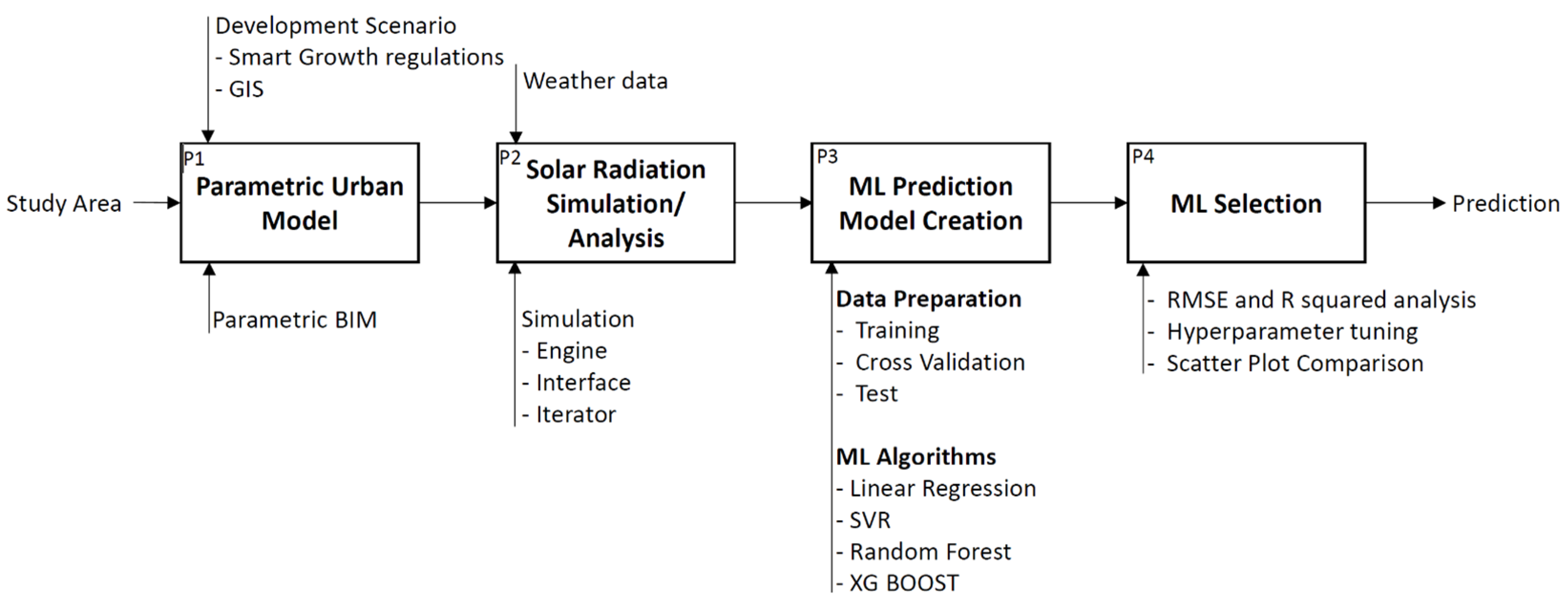
This study seeks to integrate urban modeling, energy simulation, and ML prediction to accurately represent the planned development scenarios delineated by Smart Growth regulations in the United States, with a particular emphasis on predicting solar radiation in alignment with the regulatory variables of these regulations. Figure 1 presents the overall research phases with the collected datasets, modeling and simulation techniques, and the data flow.

The primary objectives of each phase are as follows:

• Develop a parametric urban BIM that encapsulates the physical attributes dictated by Smart Growth regulations;
• Conduct iterative simulations for solar radiation, thereby generating datasets suitable for ML algorithms;
• Analyze the solar radiation simulation results based on Smart Growth regulations, generating a large dataset of individual parcels. This dataset captures significant variability in solar radiation for training the machine learning models;
• Create prediction models using multiple ML algorithms and analyze and validate their performance;
• Select the most effective prediction model within a specific context and then evaluate the applicability of the selected ML model through a case study analysis.

Subsequent sections delve into the processes and findings associated with data diagnosis and the creation/selection of the ML prediction model.

3.2. Methods, Tools, and Datasets

Each research phase in Figure 1 was carried out through specific tasks using multilayered methods, datasets, and UBES tools and techniques.

3.2.1. Data Collection from Smart Growth Regulations

The research involved the collection of (i) modeling information from GIS data for geography information and (ii) Smart Growth regulations for the planned development scenario (P1 in Figure 1).

Geography information: For the subdivision and block information, GIS shape files and attribute data were imported into a BIM. The multiple layers in GIS provided critical modeling information such as the block boundaries, subdivision shapes, traffic lanes, etc.

Information on planned development scenario: To obtain development scenario information, this study analyzed the adopted planning regulations of Smart Growth regulations. Smart Growth regulations are replacing conventional land use and zoning regulations in the U.S. They advocate strong design control of public spaces, building heights, building façade design, etc. Planned development scenarios from the regulating plan (similar to the land use and zoning map), the transect codes (similar to the land use types), and the building envelope standards were obtained.

3.2.2. Parametric Object Modeling in BIM

The next step was creating a parametric district model in the BIM (P1 in Figure 1). BIM provides an object-based library of building components and material information. This information was significant for building energy performance simulation. The robust parametric modeling mechanism in BIM enabled this study to create custom objects, allowing object geometry manipulation with parameter changes. The parametric objects in BIM can represent the simplified building mass and the buildable volumes within subdivisions. The parameter values were passed to the simulation modules to vary object geometry.

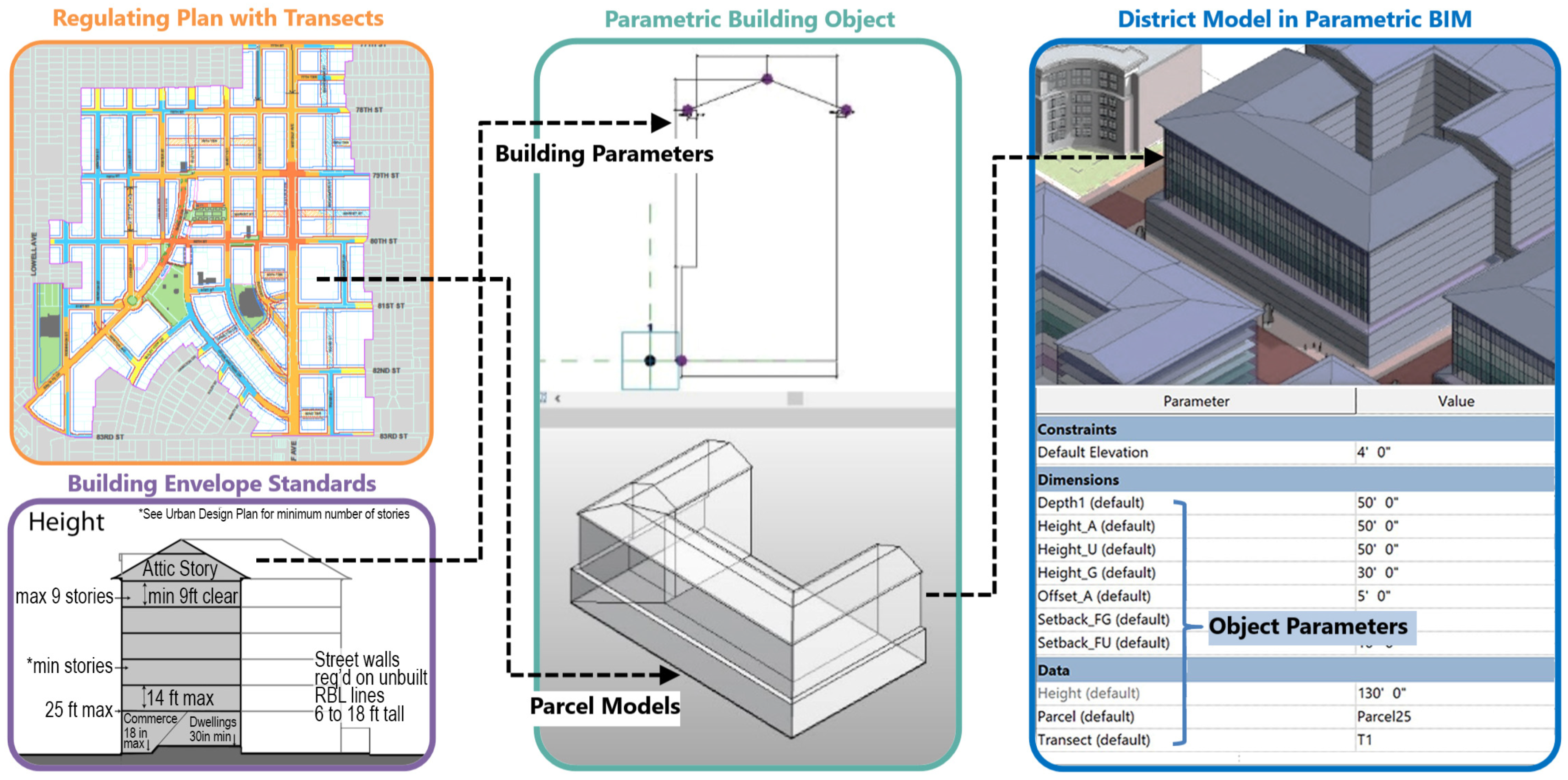
Figure 2 shows the modeling process from building envelope standards (left bottom) and the regulating plan (top left) to the parametric mass object (middle). Similar modeling techniques were applied to each parcel using custom parameter sets.

District models were built using Autodesk Revit and its custom family modeling interface. Simultaneously, the building envelope standards in the Smart Growth regulation provided the object parameter information for the building sections, ensuring that the models accurately reflect the conditions and constraints of the regulations. Further information on the parametric modeling methods is available in our previous research [5,29,30].

3.2.3. Simulation Module

Parametric simulation modules were created to iterate a large number of simulations (P2 in Figure 1). The simulation module (i) reads the object information and parameter values from BIM, (ii) iterates parameter value changes, (iii) executes solar radiation simulations, and (iv) processes the input and output data for ML prediction. The research used Ladybug and the TT Toolbox to take advantage of validated simulation engines and reliable simulation interfaces. In addition, Rhino.inside, a middleware between Revit and Rhino, was used to connect parametric BIM and the simulation interfaces. This research is built on previous works, integrating parametric BIM and multi-criteria simulations [29].

3.2.4. ML Prediction Model Creation

The creation of the ML prediction model began with simulation results generated by the simulation module. These simulations produced a substantial dataset derived from parametric variations and corresponding solar radiation outputs from the urban models.

This phase began with the partitioning of the simulation results into three sets: training, cross-validation, and test sets. This division, a standard practice in machine learning, ensures robust model selection. By training and validating models on separate datasets and subsequently testing them on previously unseen data, this approach helps mitigate overfitting and provides a fair and unbiased evaluation of a model’s performance [12].

The prediction models in this research were developed using the selected algorithms and Python (version 3.12.0) libraries, including Scikit-learn (version 1.5.1), NumPy (version 1.25.0), and Pyplot (version 3.7.2). To ensure accurate model creation and unbiased selection, several techniques were applied, including Root Mean Squared Errors (RMSEs) and R² analysis, K-fold cross-validation, hyperparameter tuning, and scatter plot comparison. K-fold cross-validation during training was employed to provide a more reliable estimate of model performance. The models were further refined through hyperparameter tuning. The following section elaborates on the detailed procedures, algorithm comparisons, and findings from the case study.

4. Implementation

The proposed framework was implemented with a case study of the Smart Growth regulations of the city of Overland Park, a southern Kansas City metropolitan area. The selected study area is one of five districts in the Vision Metcalf Plan, which was adopted to revitalize the historical corridor connecting southern satellite cities and the Kansas City downtown district. The Metcalf Plan follows the standard format of Smart Growth regulations, controlling the overall form and design of public spaces and buildings.

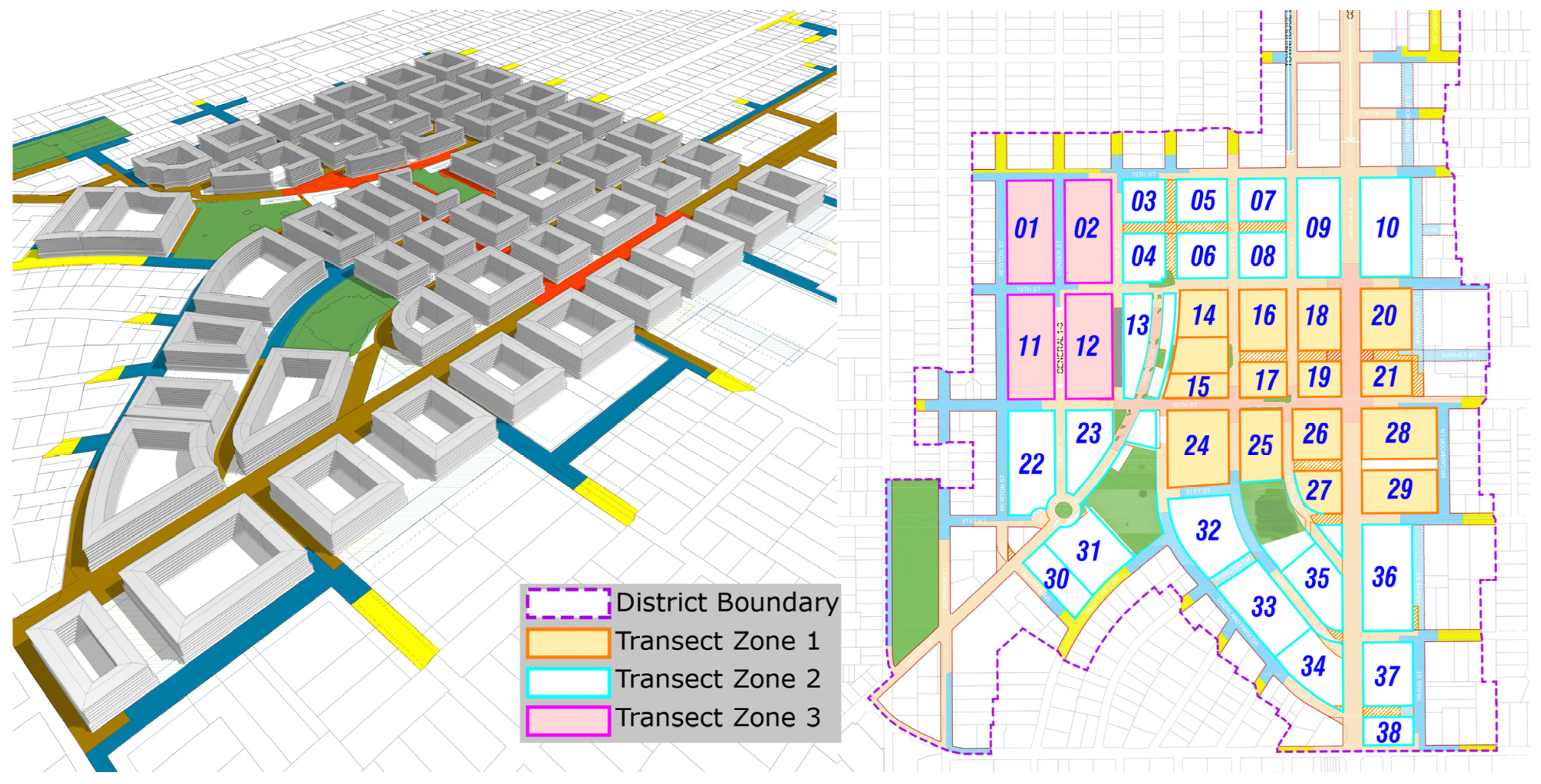
The Vision Metcalf Plan has promoted mixed-use and commercial development along the urban corridor (left). For each focused area, the Smart Growth regulations provide the development scenarios (right), the recommended building use and typologies, and the transect zone types. For each transect zone, the building envelope standards illustrate the allowed building section configuration, height, and building use. We collected the regulation information and GIS data and created a parametric district model in BIM (Figure 3). The district model (left) is a composition of custom parametric BIM objects. Each object represents the buildable building volumes within the parcels.

The Required Building Line (RBL) is the unique requirement in Smart Growth regulations that designates the specific position of the front building façade. The Regulating Plan (right) visualizes the position of the RBL, indicating the form of the BIM objects for each parcel. According to the transect zone types listed in the Regulating Plan, we formulated modeling and simulation parameters from the building envelope standards.

4.1. Iterative Simulations for Solar Radiations

This case study focused on three distinct transect zones encompassing 38 parcels. For each transect zone, parameter values were randomly assigned within the range of regulation variables outlined in the Regulating Plan and building envelope standards.

Table 1. Regulation variables of three transects for parametric BIM.

Parameters	Transect 1	Transect 2	Transect 3
Building height	7.3 m~18.2 m	7.3 m~18.2 m	7.3 m~14.6 m
Building depth	18.2 m~21.3 m	18.2 m~21.3 m	15.2 m~18.2 m
Setback	1.5 m~3 m	1.5 m~3 m	1.5 m~3 m
Roof height	2.7 m~3.6 m	2.7 m~3.6 m	2.7 m~3.6 m

presents the range of parameter values across three different transect zones. The selected parameters, including building height, depth, setback, and roof height, were crucial in shaping urban morphologies for the subsequent solar radiation simulations.

Transects 1 and 2 promote high- and mid-rise mixed-use and commercial developments, while Transect 3 recommends low-rise residential buildings. In Transects 1 and 2, the building height ranges from 7.3 m to 18.2 m, allowing considerably flexible building design within these zones. The building depth in these transects also shows a similar range, from 18.2 m to 21.3 m, allowing for variations in the building’s footprint.

The setback, the distance between the building and the property line, is between 1.5 m and 3 m in both transects, suggesting a consistent void space between the buildings. The roof height in these transects ranges from 2.7 m to 3.6 m, providing a range for the vertical dimension of the buildings. In Transect 3, building height is relatively lower, ranging from 7.3 m to 14.6 m, limiting high- and mid-rise development in residential blocks. The building depth in Transect 3 is also slightly smaller, ranging from 15.2 m to 18.2 m. However, the setback and roof height ranges remain the same as in Transects 1 and 2.

The solar radiation simulations were conducted with a high degree of thoroughness, involving 1500 iterations for each transect zone. The simulation results had a dataset of 57,000 data points across 38 parcels. These iterations were devised to represent the varying conditions within each zone, as determined by the assigned parameter values. This approach ensured a comprehensive exploration of the potential scenarios by Smart Growth regulations. After the iterative simulations, we conducted a diagnosis of the results to create ML prediction models.

4.2. Machine Learning Prediction

After 1500 simulation cases were completed, the results were divided into 900 training sets, 300 cross-validation sets, and 300 test sets to build prediction models using widely accepted algorithms, including LR, SVM, RF, and XGBoost implemented via Python (version 3.12.0) with libraries such as scikit-learn (version 1.5.1) and XGBoost (version 2.1.1). To ensure reliable performance, K-fold cross-validation, a resampling procedure commonly used for machine learning models, was employed. This method reduces bias and prevents overly optimistic estimates compared to a simple train/test split [31]. Hyperparameter tuning was also conducted to optimize predictive accuracy by calibrating model-specific parameters.

The dataset, derived from solar radiation simulations, had a low likelihood of outliers, unlike measured data in which sensor malfunctions or environmental noise might introduce anomalies. A detailed analysis confirmed no significant outliers requiring removal or transformation, further supporting the robustness of the modeling approach.

4.3. Prediction Model Evaluation

Accuracy is a critical criterion for evaluating the performance of prediction methods. This research employed various techniques to compare and enhance the performance of ML algorithms, including RMSE and R² analysis, hyperparameter tuning, and scatter plot comparisons.

4.3.1. Statistical Evaluation Using RMSE and R²

This study followed a multi-step process to identify the most accurate prediction model. The first step involved calculating the RMSE (Root Mean Squared Error) and R² (Coefficient of Determination) values for each algorithm.

The first step in the evaluation process involved calculating the RMSE (Root Mean Squared Error) and R² (Coefficient of Determination) values for each algorithm. These calculations were performed using K-fold cross-validation on both the training and cross-validation datasets to provide an initial assessment of each model’s performance. RMSE and R² are widely used statistical metrics for evaluating the performance of predictive models. They offer quantitative measures of a model’s accuracy and its ability to explain the variance in the dependent variable based on the independent variables. RMSE, which is always a positive value and is ideally close to zero, measures the average magnitude of prediction errors between the model’s predicted values and the actual target values. A lower RMSE indicates better model performance. In contrast, R² reflects the proportion of the variance in the target variable that can be explained by the model. An R² value close to 1 indicates high predictive accuracy, signifying that the model effectively captures the variability in the measured data [32].

The mathematical formulations of these metrics are as follows:

$$\mathrm{R}\mathrm{M}\mathrm{S}\mathrm{E}=\sqrt{{\displaystyle \frac{1}{n}}\sum _{i=1}^n{\left(y_i-{\widehat{y}}_i\right)}^2}$$

(1)

$${\mathrm{R}}^2=1-{\displaystyle \frac{{\sum }_{i=1}^n{(y_i-{\widehat{y}}_i)}^2}{{\sum }_{i=1}^n{(y_i-\overline{y})}^2}}$$

(2)

where

• $y_i$ represents the actual observed values;
• ${\widehat{y}}_i$ denotes the predicted values;
• $\overline{y}$ is the mean of the observed target values;
• n is the number of observations.

These metrics formed the foundation for an evaluation of the accuracy and reliability of the prediction models developed in this study.

Next, K-fold cross-validation was conducted on the training and cross-validation datasets to provide an initial evaluation of each model’s performance.

In addition, hyperparameter tuning was performed using the random search method. Hyperparameters play a critical role in machine learning models, as they control the learning process and significantly impact a model’s performance and generalization ability [20]. Unlike model parameters, which are learned from the data, hyperparameters must be set before training begins. They influence key aspects such as model complexity, learning rate, and regularization factors. Proper hyperparameter tuning can lead to more accurate and reliable predictions, while poor choices may result in underfitting or overfitting, limiting the model’s validity.

Random search contrasts with grid search, which exhaustively tests every combination of hyperparameters [20]. Instead, random search selects random combinations of hyperparameters to train the model, offering greater efficiency and effectiveness, especially when dealing with numerous hyperparameters. This approach can significantly improve the model’s predictive accuracy [33]. The combination of performance analysis and hyperparameter tuning optimized the ML models, enhancing their predictive accuracy and overall performance.

4.3.2. Visual Evaluation with Scatter Plots

Scatter plots were used as visualization tools to compare the predicted and target values derived from each algorithm. These plots provide an intuitive understanding of model performance, complementing numerical metrics such as R² and RMSE values. They are particularly useful for assessing how well algorithms capture the relationship between predicted and target measurements. A scatter plot with a clear linear pattern indicates a strong correlation between predicted and actual values, suggesting high prediction accuracy. Conversely, a more scattered or random pattern indicates lower prediction accuracy.

Through a comparison of the scatter plots of the studied algorithms, the differences in their performance were visually assessed. When combined with numerical metrics, this comparison provided a comprehensive evaluation of the ML models’ overall prediction accuracy and error rates. This approach to model evaluation ensured a more reliable and informed selection of the most accurate prediction model.

4.3.3. Model Selection

The final step in the ML process was model selection. After the models were trained and their hyperparameters were tuned, performance was evaluated using a test dataset that was not involved in the training process. This step is crucial in ML, as it provides an unbiased estimate of a model’s ability to generalize to new data. The evaluation of models on this test dataset assessed how well each model captured the underlying patterns in the data and applied this learning to unseen data. Performance metrics such as RMSE and R² were used to evaluate the models. Through this comprehensive approach, the most accurate and reliable ML model for predicting solar radiation on buildings in a district, while taking into consideration Smart Growth regulations, was identified.

5. Results

5.1. Solar Radiation Simulation Results

A substantial dataset of 57,000 data points, generated from iterative simulations, was collected and subsequently used to train the machine learning models discussed in the next section. These data points were distributed across 38 distinct parcels, providing a comprehensive dataset for analyzing solar radiation levels. The average daily solar radiation across all parcels was 2.88 kWh/m², with a standard deviation of 1.03 kWh/m², indicating considerable variation. This variation suggests that while the average daily solar radiation level was 2.88 kWh/m², actual values could deviate from this average by approximately 1.03 kWh/m². Daily solar radiation levels in the dataset ranged from a minimum of 1.07 kWh/m² to a maximum of 5.6 kWh/m², highlighting significant differences in solar radiation levels across parcels, with some receiving much more solar radiation than others.

The simulation results provided additional insights into the distribution of daily solar radiation levels. The 25th percentile was 2.06 kWh/m², meaning that approximately 25% of the solar radiation values were below this level. The median, or 50th percentile, was 2.48 kWh/m², indicating that half of the solar radiation values were below this threshold. The 75th percentile, or third quartile, was 3.88 kWh/m², meaning that about 75% of the values were below this level.

This wide range and considerable variation in the data can enhance an ML model’s ability to learn effectively by exposing it to diverse scenarios during training. Such a data pattern supports better generalization to unseen data. Additionally, the high standard deviation contributes to the model’s robustness, reducing its likelihood of being overly influenced by a small number of outliers. By training on a diverse dataset, the model is better equipped to handle a wide range of input values.

The key findings from the simulation results are summarized as follows:

• The average daily solar radiation across all parcels was 2.88 kWh/m², with a standard deviation of 1.03 kWh/m², highlighting significant variability in solar exposure across the parcels;
• The minimum and maximum solar radiation levels ranged from 1.07 kWh/m² to 5.6 kWh/m², indicating a wide range of environmental conditions and parcel characteristics;
• The 25th percentile of daily solar radiation was 2.06 kWh/m², indicating that 25% of parcels received less than this amount;
• The median (50th percentile) was 2.48 kWh/m², suggesting that half of the parcels received more solar radiation and half received less;
• The 75th percentile was 3.88 kWh/m², meaning that 75% of parcels received less than this value.

In this study, the areas were divided into three distinct transect zones, each comprising a specific set of parcels designated under Smart Growth regulations. The solar radiation levels across these zones were measured and analyzed to assess their distribution and variability (Figure 4).

Transect Zone 1 exhibits a wide range of solar radiation values. The daily mean solar radiation ranges from 1.87 kWh/m² (Parcel 26) to 4.59 kWh/m² (Parcel 24). The standard deviation, which measures variation or dispersion in the data, ranges from approximately 67.6 Wh/m² (Parcel 26) to 386.0 Wh/m² (Parcel 21). This significant variation indicates substantial differences in solar radiation across the parcels in Transect Zone 1.

Transect Zone 2 also exhibits a broad spread in solar radiation values, with a wider range of mean values compared to Transect Zone 1. The mean values range from 1.75 kWh/m² (Parcel 6) to 4.69 kWh/m² (Parcel 36), while the standard deviation spans from 118.5 Wh/m² (Parcel 6) to 446.4 Wh/m² (Parcel 31).

In contrast, Transect Zone 3 exhibits a relatively narrow spread in solar radiation values. The mean values range from 1.39 kWh/m² (Parcel 2) to 2.47 kWh/m² (Parcel 32), with the standard deviation ranging from 88.7 Wh/m² (Parcel 1) to 227.0 Wh/m² (Parcel 12). These statistics reveal noticeable differences in the distribution of solar radiation values across the three transect zones. The mean solar radiation values and their variability differ among the zones and the parcels within each zone. This variation suggests that solar radiation levels are influenced by the specific characteristics of each parcel and zone, including regulatory variables, parcel and block morphologies, and surrounding conditions.

T-tests were conducted between the transect zones to substantiate these observations. In all three tests, the p-value was less than 0.05, indicating a statistically significant difference in solar radiation between each pair of transect zones.

Table 2. T-test results among the three transect zones.

Comparison	t-Statistic	p-Value	Notes
Transect 1 vs. 2	−41.13	p < 0.05	Transect 1 has significantly lower solar radiation than Transect 2
Transect 1 vs. 3	73.38	p < 0.05	Transect 1 has significantly higher solar radiation than Transect 3
Transect 2 vs. 3	114.89	p < 0.05	Transect 2 has significantly higher solar radiation than Transect 3

presents the comparison results.

5.2. Prediction Model Evaluation Results

5.2.1. RMSE and R² Analysis

The performance of the ML models was evaluated using RMSE and R² analysis, as detailed in

Table 3. R² and RMSE of the four algorithms.

Model	Dataset	R2		RMSE
		Mean	Std.	Mean	Std.
Linear Regression (LR)	Training	0.42	0.16	43.53	23.11
	Cross-Validation	0.40	0.19	44.00	24.51
	Test	0.41	0.21	53.94	25.10
Support Vector Machine (SVM)	Training	0.65	0.15	31.30	18.94
	Cross-Validation	0.48	0.16	47.26	21.79
	Test	0.50	0.16	47.25	21.53
Random Forest (RF)	Training	0.99	0.00	4.91	2.10
	Cross-Validation	0.96	0.03	12.99	5.67
	Test	0.96	0.03	12.50	5.52
XGBoost	Training	1.00	0.00	0.15	0.06
	Cross-Validation	0.96	0.02	12.14	4.94
	Test	0.97	0.02	11.27	4.89

. To enhance model performance, hyperparameter tuning was performed using a random search during the training process. For the SVM model, tuning parameters included the kernel type (Linear and Radial Basis Function (RBF)), penalty parameter (C: 1 to 1000), kernel coefficient (gamma: auto and scale), and margin of tolerance (epsilon: 0 to 100). For the LR model, adjustments were made to the learning rate (0.0001 to 1), regularization parameter (alpha: 0.00001 to 1), and maximum iterations (max_iter: 1000 to 3000). In contrast, the RF and XGBoost models demonstrated acceptable performance without requiring hyperparameter tuning.

After the best prediction model from each algorithm was identified, a final evaluation was performed using the test dataset, which was not included in the training process. This step ensured an unbiased assessment of model performance and prevented the overestimation of accuracy due to overfitting.

The final model selection was based on the R² and RMSE metrics from the test dataset, as these provide the most unbiased estimate of model performance on unseen data. While both Random Forest (RF) and XGBoost demonstrated similar performance during cross-validation (R² of 0.96 and RMSE values ranging from 12.14 to 12.99), XGBoost outperformed RF on the test dataset, achieving an R² of 0.97 and an RMSE of 11.27, compared to RF’s R² of 0.96 and RMSE of 12.50.

These results indicate that XGBoost has a slight edge in predictive accuracy and generalization ability. Although RF showed comparable performance during training and cross-validation, the test data results confirmed that XGBoost was the best-performing model in this study. The consistent superiority of XGBoost across metrics justifies its selection for solar radiation prediction in this context.

5.2.2. Scatter Plot Comparison

Figure 5 presents scatter plots that visually depict the relationship between predicted and target values for the four ML algorithms compared: LR, SVM, RF, and XGBoost.

After hyperparameter tuning, the scatter plots for the LR and SVM models exhibited somewhat linear patterns. However, these patterns were less pronounced than those observed for the RF and XGBoost models, as reflected in the corresponding R² and RMSE values presented in Table 3. In contrast, the RF and XGBoost algorithms demonstrated the strongest linear patterns in their scatter plots, indicating high prediction accuracy. Their respective R² and RMSE values further corroborate this observation, emphasizing their effectiveness in predicting solar radiation in the given context.

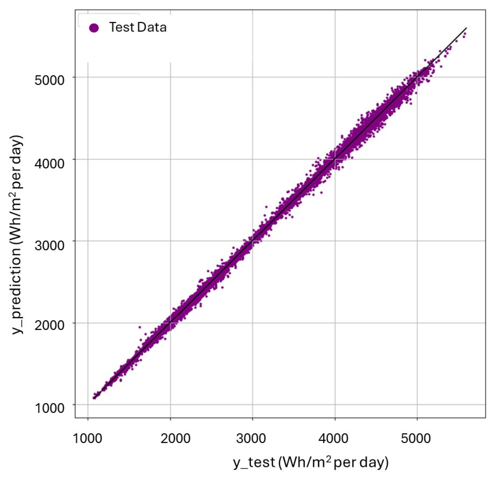
Figure 6 illustrates the performance of the selected model using test data that was not included in the training stage. This approach ensures an unbiased assessment of the model’s performance and prevents the overestimation of accuracy due to overfitting. Consistent with the R² and RMSE values, the XGBoost algorithm exhibited the most robust linear pattern across all parcels, closely followed by the RF algorithm. This observation highlights the strong predictive performance of these two algorithms. The clear linear relationship observed in the XGBoost model’s scatter plot further emphasizes its predictive strength. The model’s ability to generalize effectively across diverse parcel configurations and urban block morphologies validates its robustness in handling variability in solar radiation data. These results demonstrate that the XGBoost model, with its advanced gradient boosting techniques and regularization mechanisms, provides highly accurate predictions, making it well suited for use in the context of Smart Growth regulations within this specific urban planning scenario.

To further validate the XGBoost model and demonstrate its practical application, its predictions against solar radiation simulation results for a randomly selected set of urban design configurations across transect zones were compared.

Table 4. Comparison of solar radiation predictions from the XGBoost model with simulation results for different urban design configurations.

Parcel	Depth (m)			Height (m)			Setback (m)			Roof Ht. (m)			Simulations	Predictions
	T1	T2	T3	T1	T2	T3	T1	T2	T3	T1	T2	T3
3	21.2	21.0	15.6	13.4	11.2	10.3	2.6	2.5	2.9	2.9	2.4	2.5	2376.3	2383.3
4	21.0	19.9	17.4	15.1	18.0	13.9	1.8	2.5	2.0	3.6	1.6	3.0	1812.3	1814.4
6	19.7	19.0	17.3	15.3	12.4	9.8	1.6	2.9	1.9	3.2	2.3	3.0	1730.2	1739.9
7	20.3	21.2	15.3	14.8	11.0	10.1	2.7	2.2	2.6	3.2	2.6	2.5	2544.0	2552.8
8	21.2	18.8	17.7	14.8	9.5	7.9	2.4	1.8	2.3	3.2	2.3	1.6	2016.0	2014.6
11	18.6	19.6	15.9	7.4	12.4	13.6	3.0	2.6	2.3	2.9	1.8	2.3	1878.2	1872.6
12	18.3	20.6	16.9	16.2	17.3	13.3	2.8	2.1	2.8	3.0	2.4	2.7	1956.4	1962.2
14	19.3	19.0	16.2	12.2	16.1	9.1	1.5	2.4	2.8	3.3	1.7	2.3	2013.3	2017.7
21	20.1	20.1	17.9	9.0	12.6	12.1	2.0	2.4	2.1	2.9	1.6	2.0	4287.4	4222.9
22	19.1	20.2	17.8	9.6	11.0	7.7	1.6	1.6	2.8	3.0	2.3	2.5	4084.2	4164.8
26	19.2	20.7	16.3	14.8	9.6	8.0	2.0	2.7	2.0	3.4	2.6	2.5	1795.0	1787.4
27	19.3	18.7	17.3	17.9	12.3	12.3	1.7	2.0	2.0	2.8	1.7	2.8	3283.9	3244.8
31	18.4	20.5	16.5	18.1	10.7	11.1	2.6	2.9	1.6	3.4	3.0	2.1	3090.8	3108.1
33	19.1	19.9	17.0	13.7	13.9	14.5	2.7	2.9	2.3	3.4	3.0	2.8	1375.2	1385.2
37	20.3	21.1	15.4	13.8	9.9	7.6	2.7	1.7	2.7	3.1	3.0	1.9	5189.6	5219.4

presents the input parameters (depth, height, setback, and roof) and the corresponding predictions and simulation results. These results represent a subset of the total predictions from the XGBoost model, chosen to provide a representative comparison. The close alignment between the predicted and simulated values, with minimal deviations, confirms the model’s accuracy and applicability.

Table 4 shows the model’s ability to predict solar radiation with high precision across diverse urban design scenarios. The minimal differences between predicted and simulated values demonstrate the model’s reliability and its potential as a decision-making tool for urban planners and designers. By offering accurate predictions without the need for computationally expensive simulations, the XGBoost model facilitates the rapid assessment of energy performance under varying design configurations.

5.3. Application of the Final Machine Learning Model for Scenario-Based Predictions

Based on the solid results obtained from the analysis, particularly with the XGBoost model exhibiting the most robust linear performance, this final ML model can serve as a foundational tool for predicting solar radiation in various urban planning scenarios. One of the key advantages of this approach is that once trained and validated, the machine learning model can perform rapid predictions without requiring further time-consuming and resource-intensive simulations. This can improve efficiency, allowing urban planners, architects, and researchers to explore numerous design scenarios and their potential energy impacts in a fraction of the time previously needed.

The pre-trained model, optimized through extensive simulations, has proven to generalize well to new data. This means that it can be applied to different configurations of urban development scenarios, such as varying building heights, block layouts, and environmental conditions, without needing to re-run simulations for individual scenarios. Instead, through the inputting of the relevant urban design parameters, the model can quickly predict solar radiation levels, offering immediate feedback for decision-makers. This reduces both the computational load and the human resources required, making it a practical method for large-scale urban energy assessments.

By significantly reducing the computational and time burdens traditionally associated with urban energy simulations, the final XGBoost-based model offers a powerful tool for enhancing the decision-making process in sustainable urban planning.

6. Conclusions

This study investigated the integration of multiple ML techniques for data diagnosis, ML model creation, and prediction model comparison and selection. The proposed method successfully performed solar radiation prediction of the planned development scenarios guided by the Smart Growth regulations. The ML models successfully captured the complex interactions that affect solar radiation distribution across various urban contexts.

In the implementation phase, multiple platforms of parametric BIM, iterative simulations, and ML predictions were successfully connected. Among the various ML models studied in this research, the XGBoost model stood out for its superior performance, indicating the algorithm’s reliability for solar radiation prediction in urban environments. The research findings show the importance of appropriate ML procedures in achieving optimal model performance, including the selection of a suitable algorithm, careful data preprocessing, and the fine-tuning of hyperparameters. This research underscores the need for a systematic development approach to ML models to ensure the most accurate and reliable predictions.

Simulation results indicated that solar radiation levels were influenced by the specific characteristics of each parcel and zone, such as regulation variables and block conditions. Each transect zone had different solar radiation patterns according to varying regulation constraints, block size and orientation, buildable building volumes, adjacent building conditions, etc.

Despite these findings, the research also revealed some limitations. The performance of each algorithm varies depending on the specific parcel, and there is no one-size-fits-all solution in ML, so the algorithm selection should be carefully performed based on the specific analysis requirements, purposes, and contexts. Furthermore, this study was conducted in a specific geographical and climate context. It became possible to provide context-specific recommendations applicable to the local jurisdictions, but the results may not be generalizable to other locations. The parametric models were created based on the selected planning regulations, which are not identical to other regions’ regulations. The insights from the simulation results may not be transferable to other subdivisions. In short, further case studies could lead to improved models and more accurate predictions.

This research contributes to UBES research that utilizes ML predictions of energy performance in the urban development context. These findings will provide a novel foundation and guidelines for UBEM and UBES research, connecting building energy simulations and ML prediction algorithms to handle a large number of simulation sets. Finally, integrating these ML models with urban planning and design processes could benefit the early stage of community development. It could give stakeholders insights into how development scenarios produce environmental footprints. Planners and designers can access the ML prediction to evaluate the energy performance of what-if design scenarios. By leveraging the predictive power of these models, professionals and the public can make more informed decisions about urban development and retrofitting projects, leading to a more sustainable and energy-efficient built environment.