Experimental Study of Ambient Temperature Influence on Dimensional Measurement Using an Articulated Arm Coordinate Measuring Machine

Abstract

Articulated arm coordinate measuring machines are designed for in situ use directly in manufacturing environments, enabling efficient dimensional control outside of climate-controlled laboratories. This study investigates the influence of ambient temperature variation on the accuracy of length measurements performed with the Hexagon Absolute Arm 8312. The experiment was carried out in a laboratory setting simulating typical shop floor conditions through controlled temperature changes in the range of approximately 20–31 °C. A calibrated steel gauge block was used as a reference standard, allowing separation of the influence of the measuring system from that of the measured object. The results showed that the gauge block length changed in line with the expected thermal expansion, while the articulated arm coordinate measuring machine exhibited only a minor residual thermal drift and stable performance. The experiment also revealed a constant measurement offset of approximately 22 µm, likely due to calibration deviation. As part of the study, an uncertainty budget was developed, taking into account all relevant sources of influence and enabling a more realistic estimation of accuracy under operational conditions. The study confirms that modern carbon composite articulated arm coordinate measuring machines with integrated compensation can maintain stable measurement behavior even under fluctuating temperatures in controlled environments.

1. Introduction

Articulated Arm Coordinate Measuring Machines (AACMMs) represent a portable and flexible alternative to conventional coordinate measuring machines (CMMs), enabling fast and efficient verification of dimensions, distances, and geometric tolerances directly on the shop floor. Thanks to their jointed structure and low weight, they are easy to reposition and are therefore frequently used for inspecting larger components near machine tools or at assembly stations. Modern AACMMs are available in various lengths and configurations, and their measuring range can be further extended through optional accessories.

In contrast to conventional CMMs, which are typically operated in climate-controlled laboratories, AACMMs are often deployed in thermally unstable production environments. There, they are exposed to external influences such as air flow, radiant heat from machines, temperature changes in the measured parts, or fluctuations in ambient air temperature. These factors can cause measurement deviations, both due to changes in the measured object and due to deformation or instability of the AACMM structure. The trend of using AACMMs directly at machine tools (On-Machine Measurement, OMM), where measurements are performed under the combined effects of vibrations, thermal gradients, and rapid environmental changes is continuously growing. It is not unusual for ambient conditions to change significantly within a short time, for example, due to part heating, opening of factory doors, or altered air flow. In such applications, the metrological stability of the system becomes a critical factor.

Temperature changes can cause mechanical deformation of the AACMM—particularly thermal expansion of its segments and minor displacements in the joints. This effect was especially evident in older generations of devices, which were often made from lightweight aluminum alloys (hereafter referred to as aluminum). Aluminum offered a favorable strength-to-weight ratio and sufficient operational durability, making the AACMM relatively light and rigid. At the same time, aluminum has a relatively linear thermal expansion behavior, allowing its dimensional changes at different temperatures to be predicted and theoretically compensated. However, the relatively high thermal expansion coefficient α of aluminum meant that even small temperature variations could result in measurable errors. Earlier AACMM designs (up to the early 21st century) used aluminum segments with a thermal expansion coefficient of approximately 23 × 10⁻⁶ K⁻¹, which led to significant length errors when measuring over larger distances. Studies on these older systems demonstrated that thermal deformations often exceeded the declared accuracy of the devices unless equipped with compensation mechanisms or made from low-expansion materials [1].

Modern AACMMs typically use carbon composite components, which offer high stiffness and very low thermal expansion (with coefficients around 1–2 × 10⁻⁶ K⁻¹—an order of magnitude lower than aluminum alloys [2]). This design change significantly reduces temperature-induced mechanical deformation and improves measurement stability in environments with fluctuating temperatures. As a result, modern carbon AACMMs change their dimensions only marginally under typical temperature variations. Another advantage is the lower thermal conductivity of composite materials; the AACMM responds more slowly to sudden ambient changes and is less affected by operator body heat or solar radiation. Consequently, modern AACMM constructions better maintain their measurement stability across a wider temperature range.

Nevertheless, studies have repeatedly confirmed that even modern systems remain sensitive to thermal influences. For example, Luo et al. [2] showed that a relatively small internal temperature increase of approximately 3 °C at a laboratory ambient temperature of ~20 °C led to a length measurement error of up to 0.115 mm. After applying a regression-based compensation model, the error was reduced to 0.0335 mm. Emonts et al. [3] also demonstrated that even a high-end carbon-structured AACMM is not immune to thermal deformation during extended measurements of large parts in non-conditioned environments. The measured deformations after several hours significantly exceeded predictions based on simple linear expansion models. It is evident that AACMMs still contain metallic parts (aluminum, steel) and cannot be considered completely thermally inert, which necessitates the use of active thermal compensation methods.

The aim of this study was to experimentally verify whether a change in ambient temperature has a measurable impact on length measurements performed using the Hexagon Absolute Arm 8312, and if so, to what extent this error can be attributed to the measuring system itself. The experiment was designed so that the temperature variation occurred in a controlled manner and reflected typical workshop conditions in which the device is commonly used. Measurements were performed using a 500 mm calibrated steel gauge block, whose thermal expansion had been verified both theoretically and practically, allowing the potential influence of the AACMM itself to be isolated. Special emphasis was placed on quantifying the error component not caused by the measured object but potentially arising from thermal deformation of the AACMM structure, joint displacement, or internal sensor influence. Two measurement strategies were applied—one with slow and one with rapid temperature change—and the stabilization time of the device was also analyzed. During the experiment, ambient temperature and temperatures of the AACMM components were carefully monitored. The acquired data were evaluated using standard statistical methods and procedures based on metrology standards. The results show that while thermal changes affected the gauge block as expected, the AACMM itself provided very stable output even under significantly different thermal conditions, without a clearly demonstrable temperature dependence within the scope of the experiment. The findings contribute to a better understanding of the thermal stability of modern carbon-based AACMMs in real production environments. This topic is especially relevant for users operating such AACMMs directly as machine tools or in temperature-variable settings, who need to reliably estimate actual measurement uncertainty. The data obtained can support realistic uncertainty budgeting under operational conditions and may serve as a basis for appropriate compensation or control measures.

2. State of the Art

This chapter summarizes the current knowledge on the influence of temperature changes on the measurement accuracy of AACMM. It describes the most significant methods and models used to suppress temperature-induced errors, including empirical correction models, neural networks, linear regression methods, and advanced hybrid approaches. In addition to these academic approaches, various commercial AACMM manufacturers implement practical compensation strategies that rely on a combination of low thermal expansion materials, embedded temperature sensors, and real-time correction algorithms. The referenced studies consistently emphasize that thermal effect compensation is essential to maintain laboratory-level accuracy of AACMMs even under typical production conditions.

Santolaria et al. [1] analyzed the influence of temperature variations on the accuracy of AACMMs and developed an empirical thermal correction model based on calibration conditions set at a reference temperature of 20 °C. They demonstrated that geometric calibration alone, even at the reference temperature, does not guarantee reliable operation. At 20 °C, the maximum length error already reached 0.144 mm. The experiments used a reference ball bar standard made of carbon tube and ceramic spheres, ensuring negligible thermal expansion of the artifact. Without compensation, the measurement error systematically increased with temperature. The proposed model reduced the range of maximum errors from 175 µm to 75 µm and kept the deviation from the reference condition within ±10 µm. The model works with temperature-dependent changes in kinematic parameters while maintaining their nominal values at 20 °C, preserving the traceability of the original calibration. The study thus confirmed the necessity of thermal compensation for maintaining high accuracy under real-world conditions.

Feng et al. [4] proposed a method for compensating length errors in AACMMs using a backpropagation neural network optimized with a simulated annealing algorithm. Their model included 16 input parameters—joint angles, joint temperatures, ambient temperature, touch type, and measured length. Based on 350 training and 50 test samples collected at temperatures ranging from 18 to 22 °C, they reduced the average length error from 0.056 mm to +0.0046 mm and significantly narrowed the error range from −0.38/+0.26 mm to −0.085/+0.095 mm. The standard deviation of length also decreased from 0.172 mm to 0.037 mm. The authors concluded that thermal deformation is a key source of measurement uncertainty and can be effectively mitigated through data-driven models without affecting the original calibration.

Luo et al. [2] studied the effect of internal heating of the Hexagon Infinite 2.0 AACMM on length accuracy. Under constant laboratory conditions (~20 °C), the AACMM warmed up by 3 °C over 150 min, resulting in a maximum length error of 0.115 mm. They developed a multivariate linear regression model based on temperature differences recorded by sensors placed on the base, joints, and probe. Real-time application of this model reduced the mean length error from 0.0715 mm to 0.0335 mm, i.e., by approximately 53%. The model is simple to implement and preserves the original calibration, significantly improving reliability in non-laboratory environments.

Zhao et al. [5] proposed a two-stage length error compensation method. First, they optimized 25 parameters of the kinematic model using the Levenberg–Marquardt algorithm and data according to ASME B89.4.22-2004. Next, they applied a backpropagation neural network optimized with the Mind Evolutionary Algorithm (MEA) to compensate for remaining nonlinear errors (thermal deformation, structural deflections, shaft eccentricities). The network did not require explicit temperature inputs, as thermal effects were implicitly encoded. After full compensation, the length standard deviation decreased to 0.031 mm in experiments and to 0.010 mm in simulations, with residual errors under 0.1 mm across the measurement volume. The study proved that calibration alone is insufficient to eliminate thermal errors without adaptive correction models.

Emonts et al. [3] addressed thermal deformation of large components under non-climatized conditions. Their experiment with cast turbine housing (Ø 1425 mm) showed that simple linear models significantly underestimated real deformations. Measured expansions reached up to 160 µm, compared to an expected 60 µm. The study highlights the need to accurately compensate for anisotropic and transient thermoelastic behavior of the measured part, recommending detailed thermo-mechanical models or frequent referencing during measurement.

Samelova et al. [6] investigated the application of the Hexagon Absolute Arm 8725 AACMM for direct measurement on large CNC machines in industrial conditions. Due to the location of the measurement, particular attention was given to ambient temperature monitoring. During experiments on a HCW 3 horizontal milling center, temperature variation remained within 1 °C daily, which was deemed acceptable. However, the authors warned that seasonal fluctuations could be more significant, potentially affecting stability and measurement accuracy.

El Asmai et al. [7] experimentally determined the coefficient of thermal expansion for carbon tubes used in AACMM structures. The value was (1.13 ± 0.12) × 10⁻⁶ K⁻¹, while the effective expansion of the full assembly with aluminum end caps was 5.5 × 10⁻⁶ K⁻¹. Without this correction, a ±10 °C temperature change could cause a length error of up to 120 µm, but applying material-specific compensation reduced this error to under 25 µm. The study confirmed the crucial role of accurately determining material properties for achieving high measurement accuracy in practice.

Zhu et al. [8] proposed a dynamic error compensation model for articulated arm coordinate measuring machines (AACMM), addressing nonlinear error sources such as thermal deformation, joint angle encoding, and probe variability. By integrating temperature data from multiple sensors and applying a neural network optimized with a modified simulated annealing algorithm, the system significantly improved measurement repeatability—from 0.1782 mm to 0.0383 mm—demonstrating its effectiveness for enhancing AACMM performance under variable operating conditions.

Other types of portable CMMs also face challenges associated with temperature variations, particularly when operated outside of thermally controlled environments. In recent years, several studies have addressed this issue across various categories of equipment, including optical CMMs (OCMM), laser trackers, and portable 3D-scanning systems. These systems are frequently deployed in workshop or field conditions, where fluctuations in ambient temperature may affect both the internal stability of the device and the measured object. The following references illustrate a range of approaches to evaluating and mitigating thermally induced measurement errors.

Harmatys et al. [9] investigated the effect of machine warm-up on OCMM accuracy. Using repeated measurements over 40 h, they found that although thermal stabilization improved measurement stability slightly, all results remained within the declared maximum permissible error due to built-in thermal compensation.

Guangjie et al. [10] developed a thermal error model for a special CMM intended for use in workshop conditions. The proposed model combines multiple temperature sensors with a regression-based compensation algorithm to predict and correct temperature-related dimensional deviations. The study demonstrated that even with a limited number of sensors, noticeable improvements in measurement accuracy can be achieved.

Revilla-León et al. [11] analyzed the influence of ambient temperature variation on the dimensional accuracy of intraoral 3D scanning. Their results showed that deviations of only a few degrees from the nominal temperature range led to a significant reduction in scan trueness. The findings highlight the importance of thermal stability not only in the measuring equipment, but also in the measured object itself.

Muralikrishnan et al. [12] presented a stitching-based method for evaluating range errors in laser trackers and terrestrial laser scanners under non-ideal environmental conditions. Using overlapping measurement segments, the method allowed long-distance error evaluation (up to 120 m) without full thermal stabilization. The approach proved effective in capturing residual thermal effects and supporting corrective strategies in large-scale dimensional metrology.

Ma et al. [13] focused on thermal deformation of reference points and proposed an enhanced self-calibration and registration method for laser trackers. By modeling the thermal expansion of both the measuring setup and the measured structure, and applying weighted registration with compensation, the authors significantly improved the consistency of tracker measurements under temperature variations. The study demonstrated that combined geometric and thermal compensation enables sub-0.02 mm registration accuracy in multi-position laser tracker configurations.

Modern AACMM manufacturers implement various strategies of thermal compensation, ranging from passive design choices to integrated sensor-based correction systems. The following section summarizes the temperature compensation principles employed by three major AACMM manufacturers: Hexagon, FARO, and Kreon.

The Hexagon Absolute Arm series employs a predominantly passive compensation strategy, relying on its carbon fiber composite structure to provide excellent thermal stability across a wide temperature range. The use of low thermal expansion materials minimizes the need for active correction. Nevertheless, the arm is equipped with internal sensors for monitoring temperature and shock, which are integrated into the Hexagon RDS software system under the name SMART. This system alerts the user when significant temperature changes are detected, prompting operational caution. In addition, an external temperature sensor can be connected via the Feature Pack interface, allowing real-time monitoring of either ambient or workpiece temperature. These data can be used by the measurement software to compensate dimensional results for material expansion. While the manufacturer does not disclose the detailed algorithm of any internal correction model, the combination of passive stability and optional sensor-based input allows for high measurement reliability even under fluctuating environmental conditions [14,15].

FARO takes a more active approach, integrating semiconductor temperature sensors into each joint of its FaroArm systems. These sensors continuously measure the structural temperature of the arm and feed real-time data into the onboard processor. Based on this input, the arm’s internal software applies dynamic corrections to the kinematic model by adjusting link lengths according to the thermal expansion profile. If temperature deviations from the calibration baseline (usually 20 °C) exceed a defined threshold (±3 °C), the system warns and requires thermal stabilization before certified measurements continue. This automatic control allows the FaroArm to maintain its specified accuracy across a typical operating range of 10 °C to 40 °C, without requiring user intervention [16,17].

Kreon’s Ace arm series combines carbon composite construction with three strategically placed internal temperature sensors. These measure both structural and ambient temperature, and the arm’s controller uses these data to adjust internal parameters during operation. Kreon promotes this feature as allowing immediate use without warm-up and claims that the arms maintain measurement stability across the full range of common industrial temperatures (10 °C to 45 °C). Like the other two manufacturers, Kreon does not publicly disclose the details of the correction algorithm, but empirical compensation based on calibration at various temperatures is likely [18].

In summary, while all three manufacturers address the issue of thermal effects, they differ in their strategies. Hexagon emphasizes structural design and passive stability, with optional sensor feedback, FARO relies on comprehensive real-time internal correction, and Kreon implements a hybrid approach. These implementations are consistent with findings in the literature, which confirm that a combination of low-CTE materials and real-time thermal sensing is essential for minimizing thermal drift in AACMM measurements.

3. Research Approach

The objective of this study is to experimentally verify the influence of ambient temperature variation on length measurement results obtained using the portable measuring system Hexagon Absolute Arm 8312. The study focuses specifically on whether changes in ambient temperature can affect not only the measured object (i.e., the reference standard) but also the measuring system itself, despite the manufacturer’s declared operational temperature range of 5–40 °C. The chosen approach is based on the assumption that, even with the use of carbon composite materials and integrated compensation algorithms, thermal instability in workshop environments may still introduce distortions in the measured results.

The research design is based on an analytical approach, modeling the measuring system as a complex entity with both external and internal variables. The external variable is the ambient temperature, while the internal parameters include the structural properties of the device, measurement methodology, measured length, and the mode of operator interaction with the system. The experimental setup was designed to minimize the influence of all factors except for temperature, which was systematically varied within a defined range to isolate its impact on the measurement results.

To simulate realistic shop floor conditions, the AACMM was placed in a laboratory environment where the ambient temperature was controlled using a combination of air conditioning and a thermal source. A steel gauge block with a well-defined length was used as the reference standard and was consistently employed across all measurements. Prior to each cycle, the AACMM was kept in an idle state to avoid any additional thermal load caused by joint movement. Ambient temperature was monitored using several independent sensors and regulated with a combination of a climate control unit and industrial heating.

The measurement process was conducted in two phases. The first was a pilot phase, designed to identify temperature limits and determine the time required for system thermal stabilization. Based on the results of this preliminary stage, the main measurement phase was designed with smaller temperature increments and longer stabilization periods at each temperature level. In each regime, repeated length measurements and corresponding ambient temperatures were systematically recorded. This approach aimed to reflect real-world operational conditions that may occur in industrial settings.

The research design also included statistical analysis of the acquired data, including outlier detection, calculation of regression coefficients, and construction of uncertainty intervals. Measurement results were compared against reference values compensated according to the theoretical thermal expansion of the steel gauge block. The data analysis followed a systematic methodology, including evaluation of the correlation between temperature and measured length, and estimation of the linear component of influence, which was subsequently compared to literature values for the coefficient of thermal expansion.

This methodological approach was selected to enable a reliable assessment of whether the Hexagon Absolute Arm 8312 exhibits thermal sensitivity under controlled but industrially relevant conditions, as suggested by prior studies. Additionally, the goal was to evaluate whether the current design and internal compensation mechanisms provide sufficient protection against systematic measurement errors under variable operating conditions.

4. Materials and Methods

This section describes the equipment used, experimental setup, and measurement procedures. It provides a detailed overview of the measurement conditions, data acquisition methods, and subsequent data processing. All essential parameters required to replicate the experiment and evaluate its reliability are listed.

4.1. Equipment Used

The experimental measurements were carried out using a Hexagon Absolute Arm 8312 AACMM (Prague, Czech Republic). This is a Compact model designed for contact measurements of small- and medium-sized components. Due to its small measurement volume and fast deployment, it is particularly suitable for confined spaces, such as direct application within a machine tool workspace. Typical applications of the Compact arm include small-machined parts, medical components, or small mold cavities.

In addition to the standard certification for AACMM according to ISO 10360-12:2016, the manufacturer also provides certification in accordance with ISO 10360-2:2009, similar to conventional. For the experiment, a steel contact probe, Centre Reference Probe TKJ L 50–ø 15 mm, was installed. Measurement results were evaluated using the PC-DMIS 2023.2 metrology software. Internal temperature readings of the measuring system were obtained using the system utility software RDS 6.4. [19,20]

The technical specifications of the AACMM, in terms of accuracy and operating conditions, are presented in

Table 1. Hexagon Absolute Arm 8312-6 accuracy and size specification [15].

EUNI	PSIZE	LDIA	PFORM	Weight	Max. Reach
0.024 mm	0.01 mm	0.021 mm	0.018 mm	12.1 kg	1.49 m

and

Table 2. Hexagon Absolute Arm technical specifications [15].

Parameter	Value
Operating Temperature [°C]	5 to 40
Storage Temperature [°C]	−30 to +70
Operational Elevation [m]	Up to 2000
Relative Humidity [%]	10–90 non-condensing
Protection Rating	IP54
Marks of Conformity	CE–FCC–IC
Power Requirement [V]	110–240

. The stated accuracy values represent Maximum Permissible Error (MPE) values as defined by the acceptance test in accordance with ISO 10360-12:2016 and are specified by the manufacturer [15].

Additional instrumentation was used to monitor environmental parameters during the experiment. Two TMU USB thermometers from Papouch (Prague, Czech Republic) were employed to measure air and surface temperatures. These sensors operate within a temperature range of −55 °C to +125 °C, with a resolution of 0.1 °C and an accuracy of ±0.5 °C in the range of −10 °C to +85 °C. The devices were connected to a PC and used in combination with Papouch Wix V 1.9.5.5 software for continuous data logging.

Further environmental conditions were monitored using the LUTRON MHB-382SD (Prague, Czech Republic) instrument, which is suitable for long-term laboratory monitoring. In addition to ambient temperature, it measures relative humidity in the range of 10–95% RH with an accuracy of ±3% and a resolution of 0.1% RH. The atmospheric pressure is measured over a range of 10 to 1100 hPa with a resolution of 0.1 hPa and an accuracy of ±2 hPa.

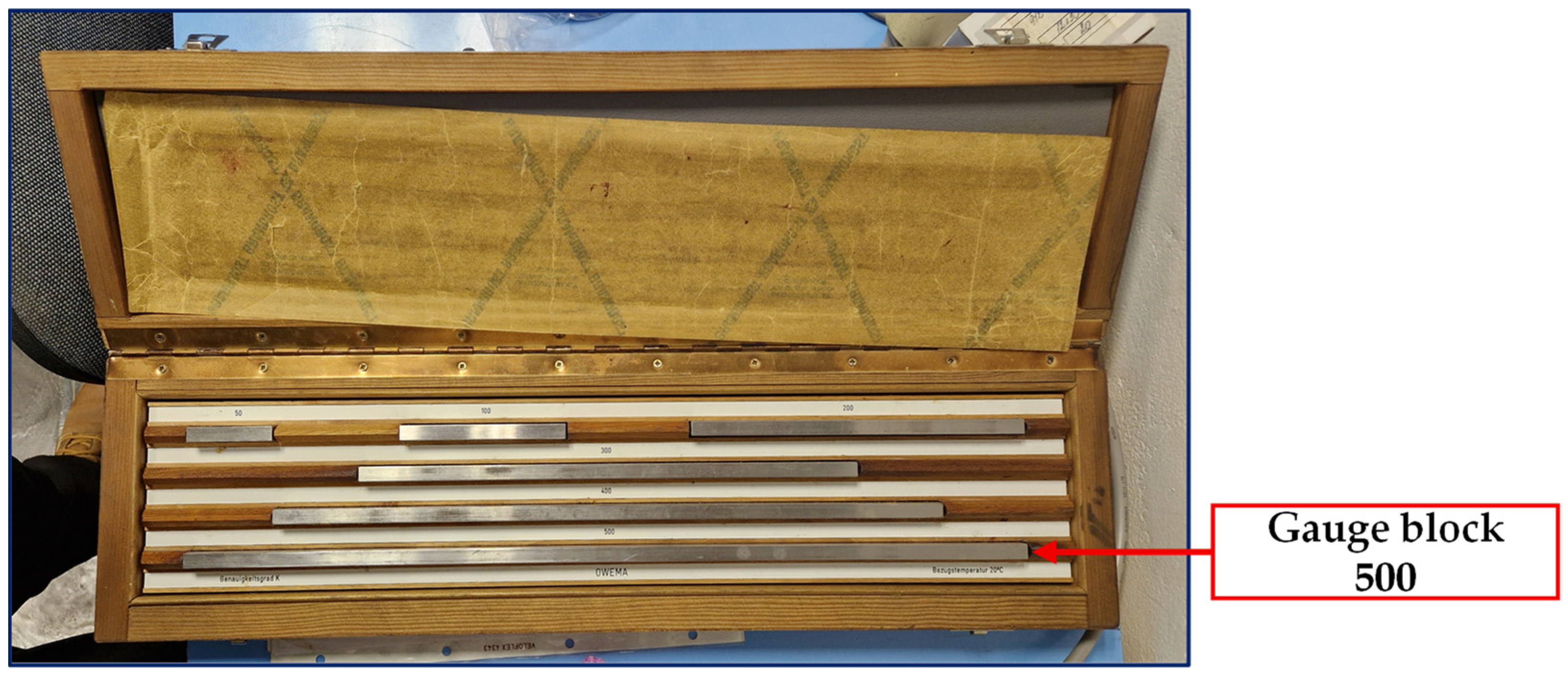
The reference standard used in this study is part of a set of steel gauge blocks (manufacturer: Hommel Hercules (Prague, Czech Republic; Grade K, range 50–500 mm), calibrated by the Czech Metrology Institute in 2011 (certificate No. 4031-KL-D0050-11). An overview of the reference standard is shown in Figure 1. 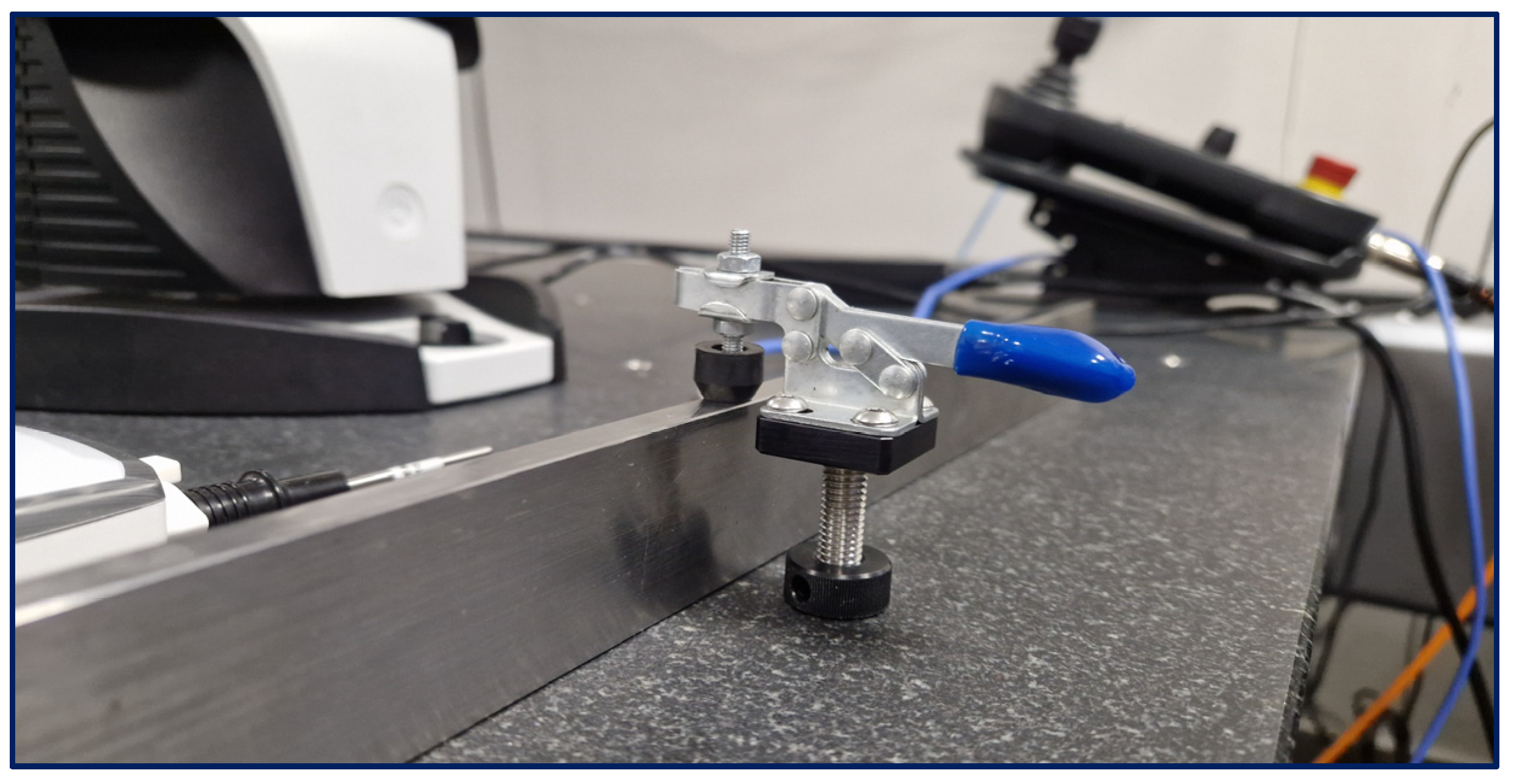For the purposes of thermal expansion calculations, a linear coefficient of thermal expansion of α = 11 × 10⁻⁶ K⁻¹ was used, corresponding to gauge blocks of larger nominal length. The gauge blocks were stored under controlled laboratory conditions in their original protective case and in the context of this experiment, they served as a stable reference for evaluating thermal effects. Its function in this study is not to provide an absolute length reference but to serve as a comparative standard for evaluating thermal effects. The gauge block was mechanically fixed to a granite metrology table using a dedicated clamping mechanism, the Hexagon Toggle Clamp (Prague Czech Republic, see Figure 2).

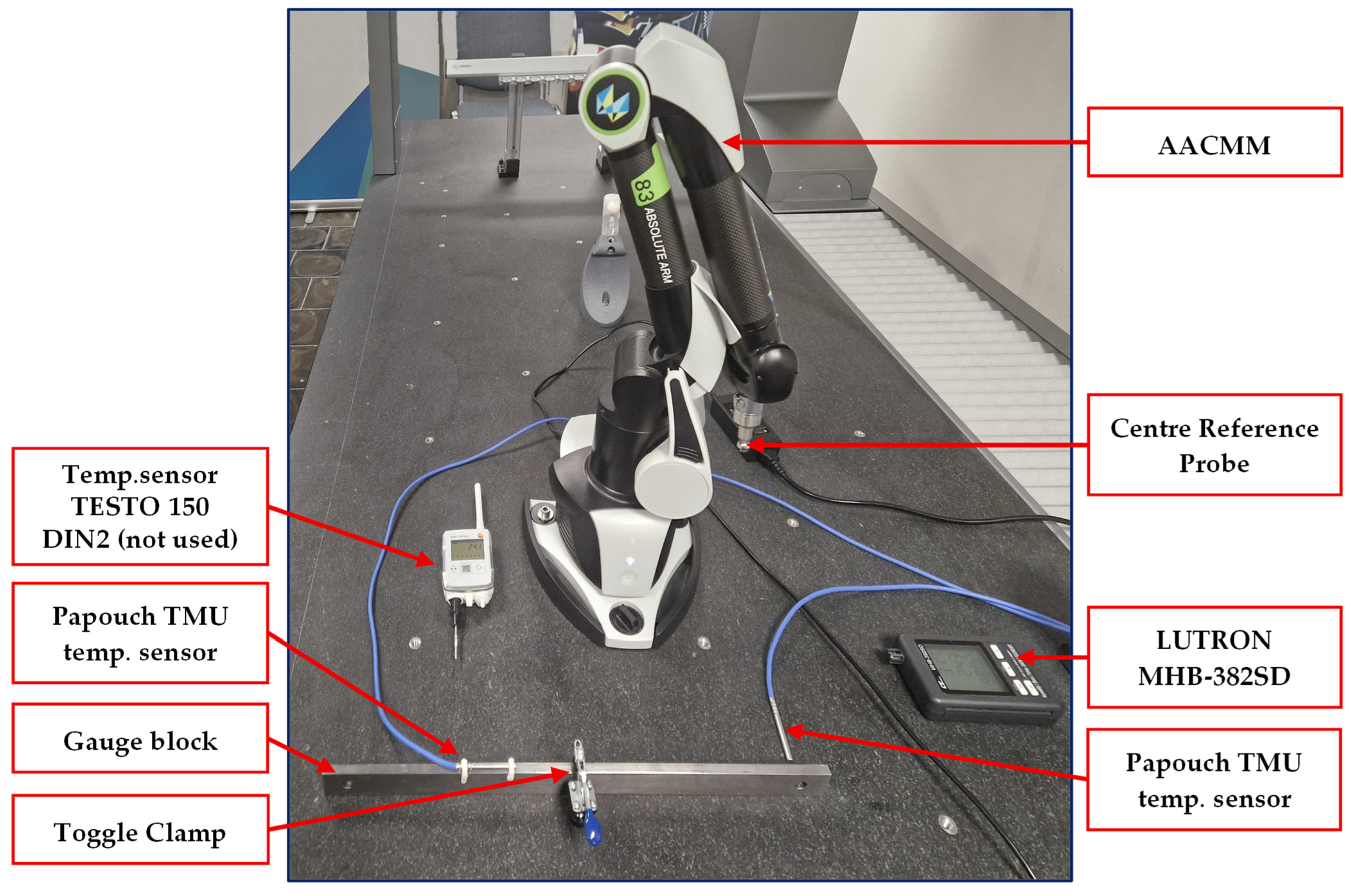
For the heating of the metrological laboratory, a 1500 W electric oil radiator was used. The room cooling was provided by a Dolceclima Air Pro 13 A+ air conditioning unit (Prague, Czech Republic). The experimental arrangement is shown in Figure 3.

4.2. Methodology

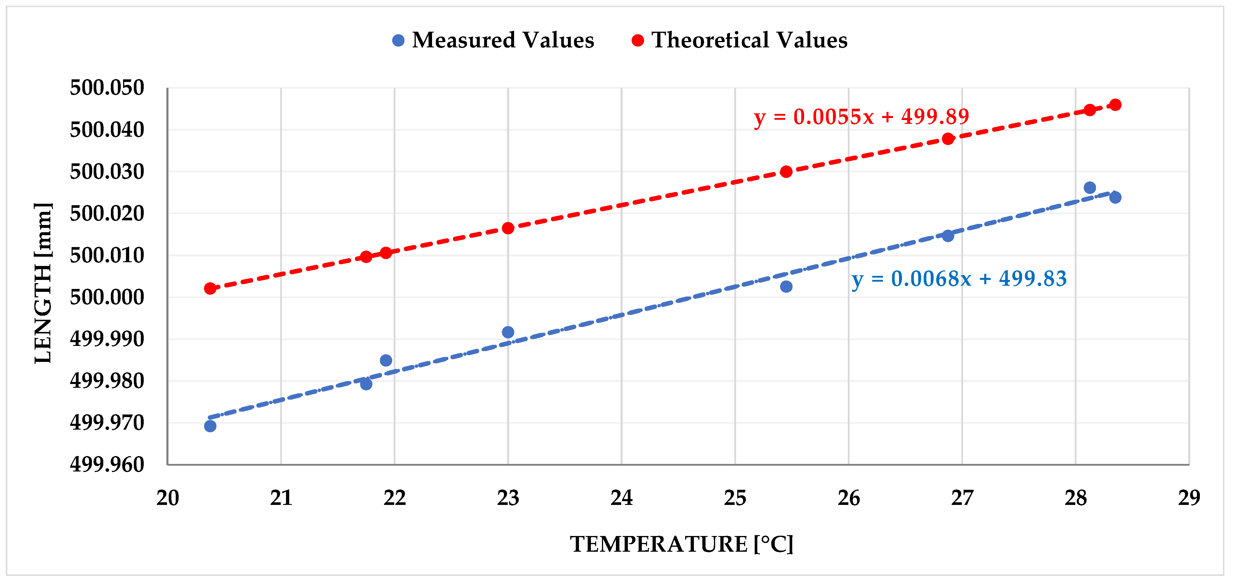
In the initial phase of the experiment, a test measurement campaign was designed with the objective of determining the achievable temperature limits, the time required for heating and cooling the laboratory, and the duration necessary for system thermal stabilization. This phase also served to test the appropriate operator position during measurement as well as the most suitable measurement strategy.

At this stage, no fixed measurement procedure was applied, temperature stabilization was not enforced, and the temperature changes occurred relatively rapidly due to the need to test the capabilities of both the electric radiator and the air conditioning unit. A portion of the measurements was also conducted under natural ambient temperature conditions in the laboratory. The pilot tests were carried out in March 2025.

Based on the evaluation of the test phase, it was concluded that the minimum and maximum achievable ambient temperatures were approximately 20 °C and 29 °C, respectively. A total of eight measurements were performed during this phase. The corresponding ambient temperatures recorded during each measurement are summarized in

Table 3. Temperatures during testing measurements.

Measurement No.	1st	2nd	3rd	4th	5th	6th	7th	8th
Temperature [°C]	20.5	21.9	22.6	22.6	23.0	25.5	26.8	28.2

.

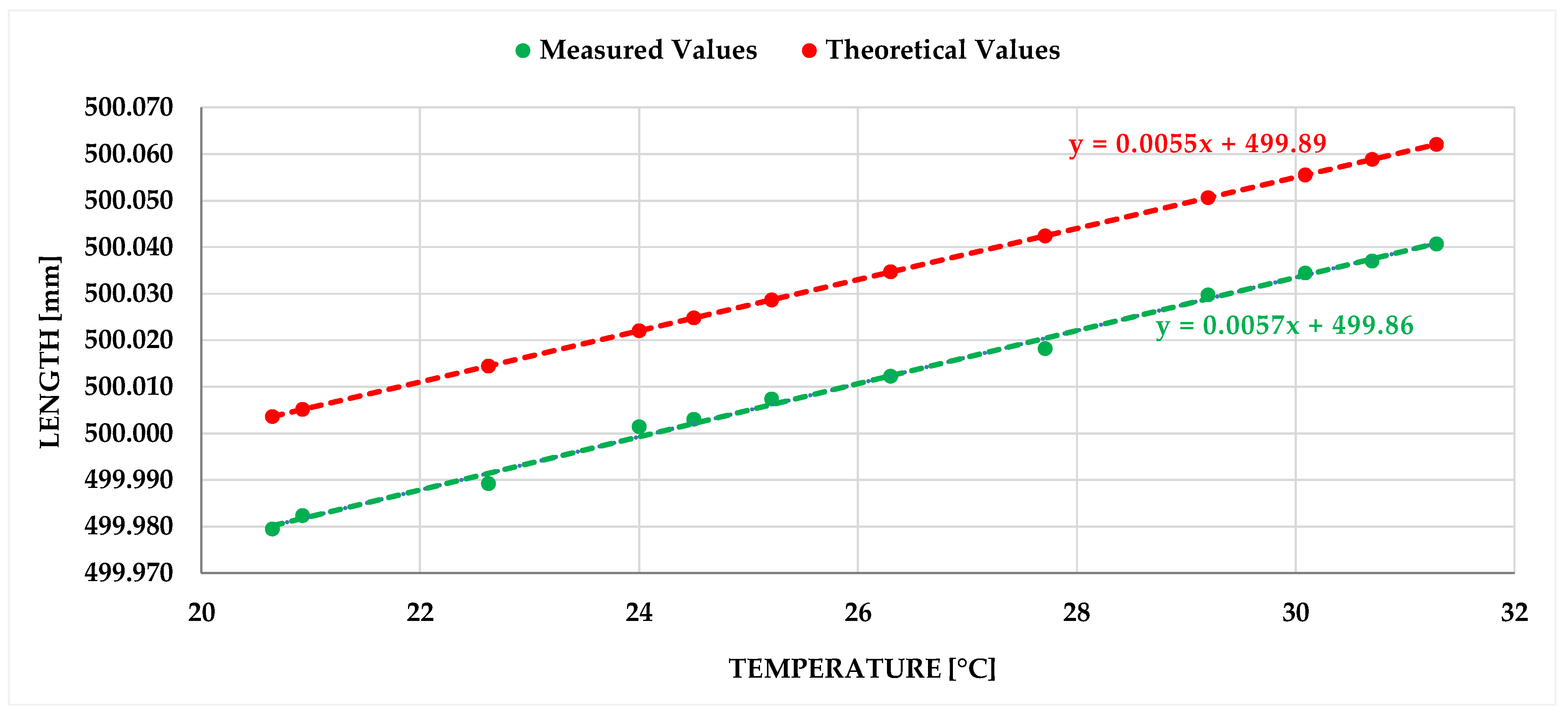
Based on the results of the test phase, a detailed measurement plan for the main experiment was established. The goal was to implement smoother temperature transitions with smaller increments and to achieve the longest possible stabilization time at each temperature level. Given the experimental objective of evaluating the temperature dependence of measurement results, the aim was to cover as many temperature levels as possible within the selected range (approximately 20–29 °C).

The methodology included two measurement blocks per day, spaced 12 h apart. A single 12 h block was considered sufficient to allow thermal equilibrium between the ambient air, the AACMM, and the steel gauge block. Continuous temperature monitoring was essential for ensuring environmental stability. Therefore, two Papouch TMU thermometers were used—one placed in the measurement zone and the other mounted directly onto the gauge block.

The laboratory environment was carefully controlled to avoid undesired thermal transitions, and the system was considered thermally stabilized when the temperature variation did not exceed 0.2 °C [1]. The shortest recorded thermal stabilization time was 3 h and 6 min, while the longest stabilization time occurred at the maximum temperature level and lasted 12 h and 6 min.

The temperature levels at which the final measurements were performed are listed in

Table 4. Measurement timetable with temperature and activity log.

Day	Time	Activity	Temperature [°C]
Friday	17:30	Heating started	24.2
Monday	8:00	1st measurement; change in temperature	31.3
	20:00	2nd measurement; change in temperature	30.7
Tuesday	8:00	3rd measurement; change in temperature	30.1
	20:00	4th measurement; change in temperature	29.2
Wednesday	8:00	5th measurement; change in temperature	27.7
	20:00	6th measurement; change in temperature	26.3
Thursday	8:00	7th measurement; natural cooling	25.2
	20:00	8th measurement; natural cooling	24.5
Friday	8:00	9th measurement; A/C cooling	24.0
	20:00	10th measurement; A/C cooling	22.6
Saturday	8:00	11th measurement; A/C cooling	20.9
	20:00	12th measurement	20.7

.

A simple measurement program was created in the PC-DMIS software. The length of the gauge block was evaluated as the distance between two planes. Each measurement at a given temperature level was repeated 12 times to ensure statistical reliability.

4.3. Theoretical Basis

Thermal drift represents one of the main systematic sources of uncertainty in AACMMs. This phenomenon arises due to variations in ambient or internal temperature, which cause thermal expansion or contraction of the structural components of the arm—primarily its segments and joints. Since these parts are typically made of metals or composite materials with non-zero coefficients of thermal expansion, heating or cooling leads to slight geometric deformation of the arm. Although not directly observable during operation, this deformation causes the measured coordinates to gradually shift over time, even if the measured object remains stationary and the arm is not moved.

Thermal drift is typically time-dependent—it becomes more pronounced during transient phases after power-on or temperature fluctuations, before thermal equilibrium is achieved. It may be caused not only by environmental changes but also by internal heat generation in components such as motors, encoders, or bearings, which results in thermal gradients across the arm. These gradients lead to non-uniform mechanical behavior and difficult-to-predict structural deformations. The result is a discrepancy between the actual and indicated position of the probe tip, which can reach several tenths of a millimeter even under small temperature variations.

Since this is a systematic effect, it cannot be eliminated by simple repetition of measurements. Thermal drift thus has a significant impact on both accuracy and repeatability, and in longer measurement sequences, it may lead to incorrect conclusions about the dimensional properties of the measured part. To mitigate this effect, AACMMs are equipped with various structural and algorithmic compensation mechanisms. On the structural side, materials with low thermal expansion coefficients, such as carbon fiber composites, are commonly used. In addition, a set of integrated temperature sensors is often embedded in the arm, enabling software-based thermal compensation using empirical or regression-based models, or more recently, neural network. However, the exact principles of these algorithms are typically not disclosed by manufacturers.

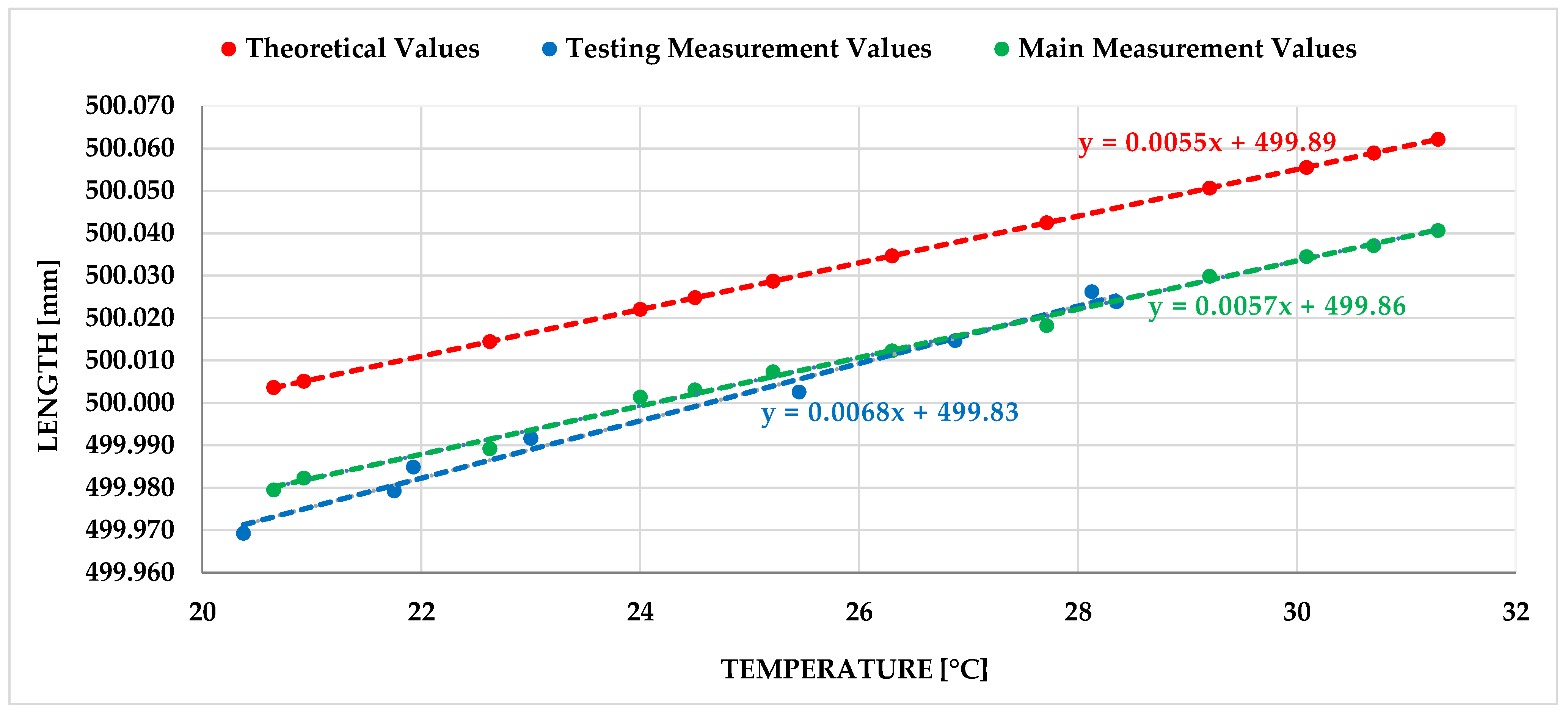
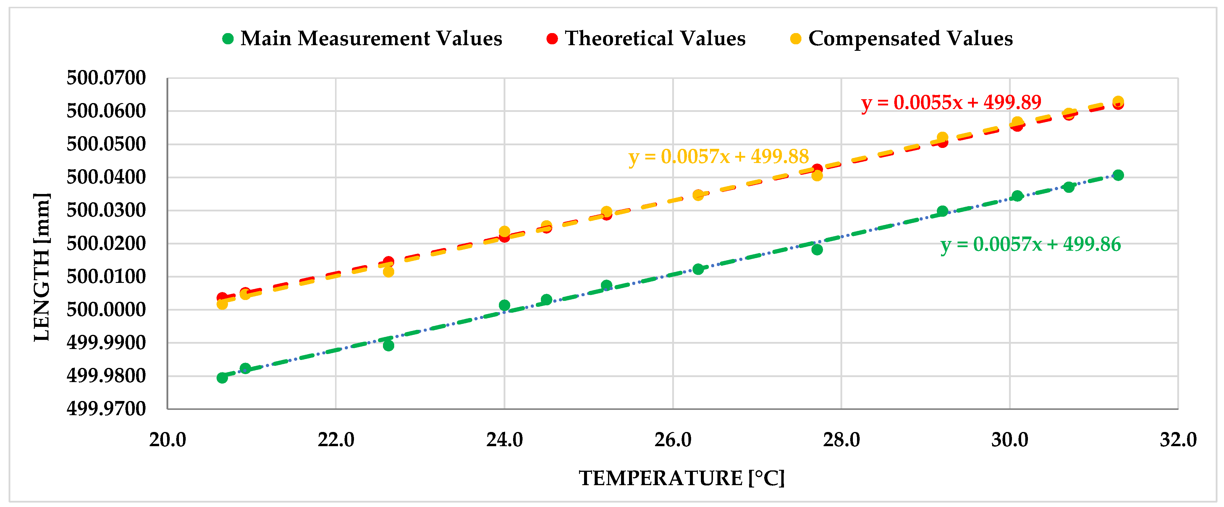
To evaluate the dependence of the measured length on ambient temperature, the method of linear regression was selected, as most engineering materials exhibit approximately linear thermal expansion within the typical range of technical temperatures. The linear regression model describes the relationship between the independent variable (temperature) and the dependent variable (measured length) in the following form:

$$y={\beta }_{1}x+{\beta }_0,$$

(1)

where β₁ represents the slope of the regression line and β₀ its intercept with the y-axis. In the context of this analysis, the slope has a clear physical interpretation as the effective thermal expansion coefficient of the entire measurement path, i.e., not only the gauge block but also the associated components of the measuring system. The intercept corresponds to the hypothetical length at zero temperature and may indicate a systematic offset or calibration error.

The linear model thus enables the quantification of the difference between the theoretical expansion of a known material and the actual measured value, which can reveal, for example, thermal dilation of the AACMM or other mechanical influences. The model also serves as a basis for further calculations, such as estimating the effect of temperature variations on measurement uncertainty or designing compensation coefficients. The quality of the fit was assessed using the coefficient of determination R², which expresses to what extent the data variability can be explained by the regression model. A high value of this indicator confirms the suitability of the chosen approach and supports the assumption of linear dependence within the specified conditions.

In this study, the regression equations are presented as deterministic lines without an explicit residual term. Deviations in individual data points from the model were considered only through the calculation of the R² value. The resulting equations thus serve primarily to interpret trends and compare them with theoretical models. Type A uncertainty was not derived from the residuals of the regression analysis but was determined independently based on repeated measurements, as the standard deviation of the mean, in accordance with the GUM recommendations [21]. This approach corresponds to common metrological practice, where the goal is to quantify the statistical dispersion of measured values regardless of the applied dependency model.

After evaluating the dependence of the gauge block length on ambient temperature using the linear regression model, the next objective was to determine the measurement uncertainty throughout the experiment. The measurements were conducted under laboratory conditions in order to simulate typical usage of the measuring device at various temperatures, with an emphasis on assessing the influence of the AACMM itself. It is assumed that if the gauge block has a known thermal expansion coefficient, any additional length changes due to temperature variation can be attributed to the measuring system—i.e., the AACMM and other components. This assumption is particularly important in cases where direct calibration of the measuring device at different temperatures is not available or where it is necessary to estimate the expanded uncertainty under current conditions. In this analysis, type A uncertainty was determined according to GUM recommendations as the standard deviation of the mean from repeated measurements. A potential systematic influence of the AACMM, demonstrated by the regression analysis, would be considered as a component of type B uncertainty.

In the calculation of measurement uncertainty, the standard procedure according to GUM was followed, taking into account the information provided by Moona et al. [21,22]. In practical processing and evaluation, the required quantity is ideally measured at least ten times, under the assumption that the components forming the combined standard uncertainty u_c follow a normal probability distribution N(μ,σ²). From the measured dataset x_i, the arithmetic mean is calculated according to Equation (2).

$$\overline{x}={\displaystyle \frac{{\sum }_{i=1}^n{x}_i}{n}},$$

(2)

The type A standard uncertainty u_A depends on the number of measurements n performed and decreases as the number of measurements n increases. For independent (uncorrelated) measured values, u_A is related to the sample mean and is calculated using Equation (3), which defines the standard deviation of the sample mean. Equation (3) may alternatively be expressed in terms of the sample standard deviation s_x.

$$u_A=s\left(\overline{x}\right)=\sqrt{{\displaystyle \frac{{\sum }_{i=1}^n(x_i-\overline{x}{)}^2}{n\left(n-1\right)}}}={\displaystyle \frac{s_x}{\sqrt{n}}},$$

(3)

The uncertainty u_A is caused by the variation in measured values. In the case of a small number of measurements (n < 10), the value determined by Equation (3) is not very reliable. If the measurement uncertainty is to be evaluated using the type A method according to GUM, measurements should be repeated at least 10 times. In Czech literature, there is a procedure based on TPM 0051:93 Determining Uncertainties in Measurements for n ≥ 2, which was also applied in this calculation [23]:

$$u_A=K.s\left(\overline{x}\right),$$

(4)

where the values of the correction coefficient K depend on the number of measurements n and are given in

Table 5. Correction coefficient K values for type A uncertainty adjustment.

n	2	3	4	5	6	7	8	9	10	11	12
K	7.0	2.3	1.7	1.4	1.3	1.3	1.2	1.2	1.0	1.0	1.0

.

To calculate the combined standard uncertainty u_C, it is also necessary to determine the type B uncertainty u_B. The uncertainty u_B does not depend on the number of measurements but is derived by standardizing the possible sources of uncertainty z_j. The individual components of uncertainty that form u_B are identified under the assumption that they are uncorrelated.

$$u_B=\sqrt{{\sum }_{j=1}^m{u}_{zj}^2},$$

(5)

or each source, a range of deviations ±Δz_jmax from the nominal value is estimated in such a way as to minimize the probability of exceeding the interval. Furthermore, the probability distribution corresponding to the deviations Δz within the interval ±Δz_jmax is assessed, and the individual uncertainties u_zj (i.e., the contributions to the type B uncertainty u_B) are determined.

$$u_{zj}=c_j{\displaystyle \frac{\mathsf{\Delta }{z}_{jmax}}{\chi }},$$

(6)

where the coefficient c_j denotes the sensitivity coefficient and the value χ is determined based on the selected approximation. The values of χ correspond to the ratio ${\displaystyle \frac{{∆z}_{jmax}}{\sigma }}$ where σ² is the variance of the respective distribution, as listed in the following overview:

• χ = 3 (2) for a normal distribution,
• χ = $\sqrt{6}$ for a triangular (Simpson’s) distribution,
• χ = $\sqrt{2}$ for a bimodal triangular distribution,
• χ = 1 for a bimodal Dirac distribution,
• χ = $\sqrt{3}$ for a uniform (rectangular) distribution,
• χ = 2.04; 2.19; 2.32 for a trapezoidal distribution.

The standard combined uncertainty u_C is calculated from the type A and type B uncertainties under the assumption that the input quantities are uncorrelated. The calculation is performed according to Equation (7):

$$u_c=\sqrt{(u_A^2+u_B^2)}.$$

(7)

In the case of an AACMM, the foundation of its inherent uncertainty is determined during the manufacturing and assembly of the system itself. Errors originating from individual AACMM components—such as systematic encoder errors—accumulate during both measurement and calibration. The uncertainties of an AACMM can generally be divided into two main categories:

• Kinematic errors, which are related to the physical structure and motion of the AACMM. These include inaccuracies in segment lengths, where the actual segment length differs from that defined in the kinematic model. Further sources are twisting errors, manifesting as deviations in segment orientation, and errors in the zero position, referring to inaccuracies in defining the initial AACMM position. These factors have a significant impact on the accuracy of position and orientation determination.
• Non-kinematic errors, which result from factors independent of the AACMM’s kinematics. Deformations of the segments due to their own weight or external forces may cause shifts in measured points. Temperature-induced errors—arising from dimensional changes caused by thermal expansion of the AACMM components—can substantially affect measurement accuracy, especially in environments with fluctuating temperatures.

Given that an AACMM is a portable measurement system (MS) designed for use in various, often demanding, metrological environments, these conditions significantly affect the measurement uncertainty. Temperature fluctuations are particularly critical and must be taken into account when determining the final measurement uncertainty. This assumption is fundamental to this study. Humidity and atmospheric pressure may influence the AACMM’s electronic components, which is why these parameters were also monitored throughout the measurements. However, current AACMMs are commonly rated up to IP54 protection level by manufacturers, indicating that the system itself is not critically affected by humidity. This also applies to dust and contamination. In dusty environments, it is necessary to clean both the part and the measuring probe to minimize the impact of contamination on the measurement uncertainty.

In typical industrial applications of AACMMs, it is also important to monitor vibrations and shocks, which can lead to instability and measurement errors. Since this study was conducted in a laboratory environment, this source of uncertainty was not considered.

Because AACMMs are manually operated systems, the operator is an essential source of uncertainty. The user’s experience and knowledge of the equipment also play a key role in minimizing errors and ensuring consistent results. Human factors contributing to uncertainty include the applied probing force, measurement stability, selection of probe points, probe orientation, and measurement strategy. This influence was evaluated during the preliminary testing phase and minimized by selecting an experienced operator, an appropriate working position, and a suitable measurement strategy.

Another factor playing a crucial role in measurement accuracy and uncertainty is the probing system. Inaccuracies of tactile probes can result from manufacturing tolerances, wear, or improper calibration. These errors can lead to significant deviations in measurement results, particularly when measuring small or complex geometries. For the experiment, a Center Reference Probe was selected due to its high stiffness and presumed accuracy. Considering the known thermal expansion coefficient of steel and the stylus length, the thermal contribution of the probe was estimated to be an order of magnitude smaller than other primary components of the combined uncertainty. Therefore, it was considered negligible in this study.

A theoretical source of uncertainty when using AACMMs is also the selection of the metrological software used for processing and evaluating measured data. The software algorithms that process data from the probe can potentially contribute to measurement uncertainty. However, the developers of major reliable metrological platforms used with coordinate-measuring equipment currently state that the influence of the software itself on measurement results is negligible. This source of uncertainty was therefore not considered in this study [22,24,25,26,27,28].

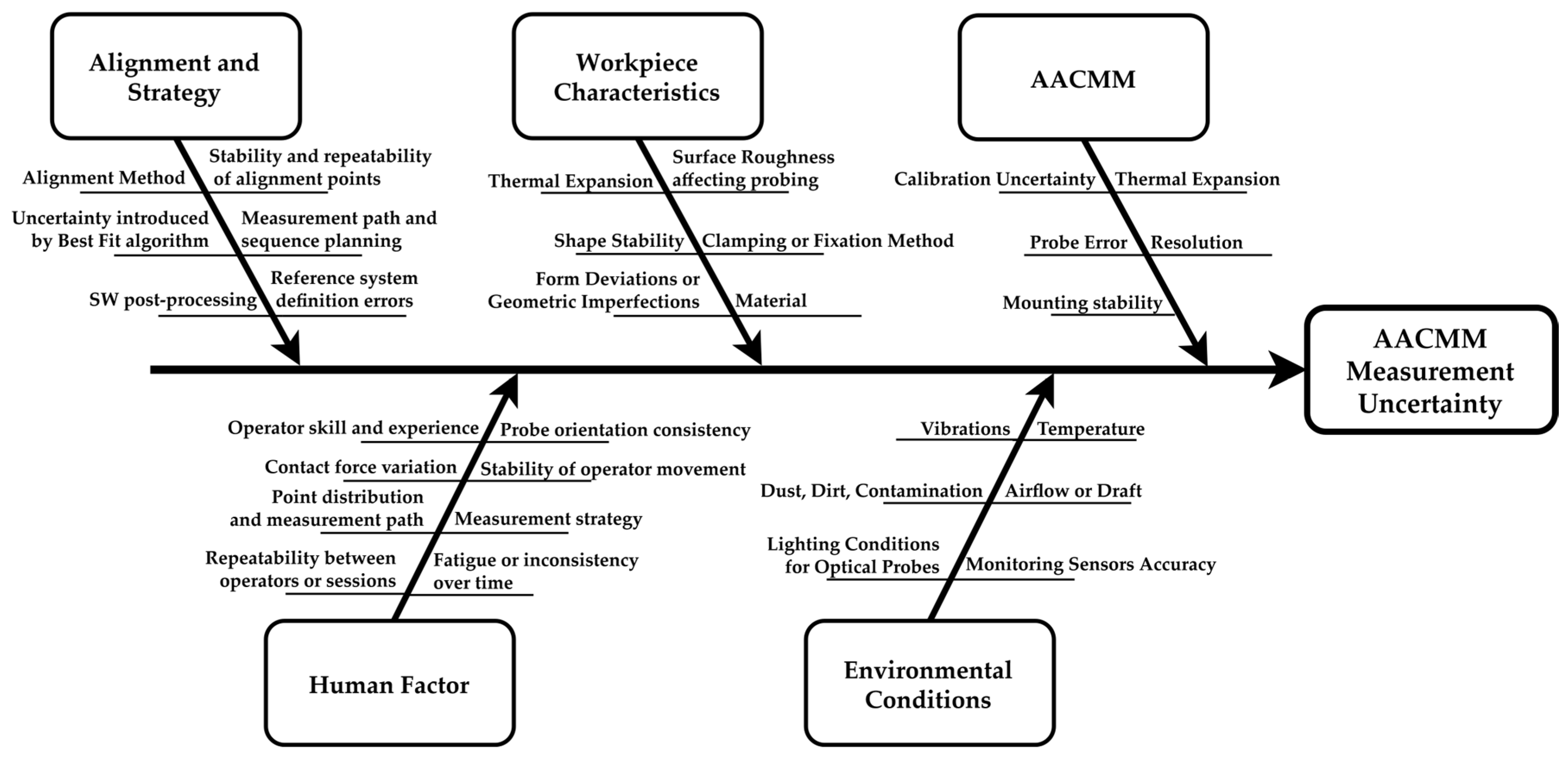
The fishbone diagram in Figure 4 illustrates the potential sources of type B uncertainty in measurements performed with an AACMM.

4.4. GenAI Used

Generative artificial intelligence (GenAI), specifically ChatGPT-4o (OpenAI), was utilized in this manuscript to translate and interpret content from the original Chinese-language article by Luo et al. [2]. While the primary interpretation and contextual framing of Luo et al.’s work were based on the English abstract provided by the original authors, GenAI was used to translate and clarify detailed information from the main body of the Chinese text. Due to language limitations, authors relied on the accuracy of this AI-assisted translation for detailed content. Additionally, GenAI was employed for linguistic revisions and grammar checking of the English manuscript.

5. Results

This chapter summarizes the results of the experiment, demonstrating the influence of temperature changes on length measurements using an AACMM. It presents the measured values, their evaluation, graphical representations, and the derived characteristics of the system. The results are further interpreted in terms of measurement uncertainty, residual errors, and the metrological relevance for practical use in typical industrial environments.

5.1. Test Measurement Results

Table 6. Measured lengths corresponding to specific temperatures during the test measurements.

	1	2	3	4	5	6	7	8
	20.5 °C	21.9 °C	22.6 °C	22.6 °C	23.0 °C	25.5 °C	26.8 °C	28.2 °C
DIST1	-	499.962	499.952	499.975	500.022	500.012	500.014	500.000
DIST2	-	499.958	499.979	499.981	500.026	500.025	500.014	500.000
DIST3	499.978	499.856	499.977	499.983	500.027	500.023	500.015	499.997
DIST4	499.982	499.973	499.978	499.985	500.027	500.023	500.016	500.005
DIST5	499.997	499.973	499.978	499.985	500.028	500.024	500.015	500.008
DIST6	499.993	499.973	499.990	499.985	500.025	500.023	500.014	500.004
DIST7	499.989	499.962	499.980	499.986	500.028	500.024	500.014	499.998
DIST8	499.999	499.974	499.980	499.984	500.026	500.018	500.016	500.005
DIST9	499.999	499.975	499.979	499.984	500.028	500.023	500.014	500.000
DIST10	499.996	499.973	499.967	499.986	500.025	500.025	500.013	499.986
DIST11	-	-	499.981	499.986	500.026	500.025	500.016	500.012
DIST12	-	-	499.981	499.985	500.021	500.023	500.015	499.999
$\overline{\mathrm{x}}$ [mm]	499.9916	499.9692	499.9792	499.9849	500.0262	500.0238	500.0147	500.0025

presents the results of the test length measurement at eight different temperatures, ranging from 20.5 °C to 28.2 °C. The values highlighted in light gray were identified as outliers. For the temperatures 20.5 °C and 21.9 °C, fewer data points were recorded due to the exploratory nature of the initial test runs. Both data series exhibit a clear linear trend in the dependence of length on temperature. The gauge block’s behavior corresponds to the expected thermal expansion of the material, while the measurements obtained using the AACMM show a systematically higher response, indicating an additional influence from the measuring system itself.

For the AACMM measurements, linear regression analysis yielded a slope of 0.0068 mm/°C, which is approximately 1.3 µm/°C higher than the expansion predicted by the gauge block alone. The reference regression line for the gauge block was calculated theoretically based on a gauge block reference value of 500.00052 mm and a linear thermal expansion coefficient of α = 11 × 10⁻⁶ K⁻¹, as stated in the calibration certificate. This resulted in a theoretical slope of 0.0055 mm/°C.

The difference between the AACMM’s regression slope and the theoretical value for the gauge block implies that approximately 19% of the total length increase per 1 °C can be attributed to the additional influence of the measuring system. This deviation may result from the mechanical properties of the AACMM, its own thermal expansion, or inaccuracies in the device’s kinematic model.

The coefficient of determination for the AACMM regression model is R² = 0.987, confirming a strong linear correlation and supporting the use of a regression-based approach. The observed difference in the y-intercepts of the two regression lines (499.89 mm for the theoretical gauge block and 499.83 mm for the AACMM) indicates a systematic offset, which may be related to the coordinate system initialization, calibration error, or mechanical characteristics of the AACMM itself.

Figure 5 illustrates the difference between the ideal (theoretical) behavior of the gauge block and the actual temperature-induced response of the AACMM. It shows that the discrepancy lies not only in the slope but also in the absolute offset. This insight is important for further analysis of the type B uncertainty components.

5.2. Main Measurement Results

Table 7. Measured lengths corresponding to specified temperatures during the main measurements.

	1	2	3	4	5	6	7	8	9	10	11	12
	31.3 °C	30.7 °C	30.1 °C	29.2 °C	27.7 °C	26.3 °C	25.2 °C	24.5 °C	24.0 °C	22.6 °C	20.9 °C	20.7 °C
DIST1	500.039	500.037	500.035	500.027	500.012	500.014	500.003	500.001	500.001	499.988	499.983	499.981
DIST2	500.040	500.036	500.035	500.031	500.020	500.012	500.006	500.004	500.002	499.991	499.983	499.979
DIST3	500.042	500.038	500.033	500.031	500.021	500.011	500.012	500.003	500.002	499.991	499.982	499.981
DIST4	500.040	500.038	500.035	500.030	500.018	500.013	500.008	500.002	500.003	499.991	499.981	499.980
DIST5	500.040	500.038	500.034	500.028	500.016	500.013	500.009	500.002	500.001	499.990	499.982	499.979
DIST6	500.039	500.036	500.034	500.028	500.019	500.014	500.004	500.002	500.001	499.990	499.982	499.979
DIST7	500.031	500.037	500.035	500.032	500.021	500.012	500.007	500.004	500.002	499.988	499.981	499.979
DIST8	500.042	500.036	500.035	500.031	500.023	500.012	500.011	500.004	500.000	499.989	499.983	499.979
DIST9	500.040	500.037	500.035	500.029	500.011	500.011	500.005	500.003	500.002	499.989	499.985	499.980
DIST10	500.041	500.036	500.033	500.031	500.017	500.011	500.006	500.003	500.000	499.989	499.984	499.980
DIST11	500.042	500.037	500.037	500.030	500.021	500.012	500.010	500.004	500.001	499.988	499.979	499.978
DIST12	500.042	500.038	500.038	500.029	500.019	500.012	500.007	500.004	499.997	499.986	499.982	499.978
$\overline{\mathrm{x}}$ [mm]	500.041	500.037	500.035	500.030	500.019	500.013	500.008	500.003	500.002	499.989	499.982	499.979

presents a summary of the main measurement campaign, performed at 12 temperature levels with 12 repetitions at each level. Values highlighted in light gray were identified as outliers and were excluded from further calculations. The measured values once again confirm a strong linear dependence of the gauge block length on ambient temperature.

Linear regression applied to the average values yielded a slope of 0.0057 mm/°C and an intercept of 499.86 mm, indicating that the measured length increases by approximately 5.7 µm for every 1 °C increase in temperature. This result is in good agreement with the theoretically expected expansion of the steel gauge block (0.0055 mm/°C), with a relative difference of only 3.5%. These findings are illustrated in Figure 6.

From a statistical perspective, the regression model demonstrates a high degree of agreement (R² = 0.996, R = 0.998), confirming that nearly all variability in the measured length can be explained by changes in temperature. These results provide a reliable basis for the subsequent uncertainty analysis and confirm that the system exhibits predictable behavior consistent with the theory of linear thermal expansion.

Figure 7 shows a comparison between the main and test measurement results and demonstrates that, despite a slightly different slope, the trend remains stable and approximately linear in both cases.

5.3. Data Offset Compensation

Figure 8 shows a direct comparison between the measured length values, the theoretical expansion model, and the compensated data. The graph clearly illustrates that the actual values from the main measurement (green line) are systematically lower across the entire temperature range compared to the corresponding theoretical values (red line). This offset averages at 22.3 µm and remains virtually constant regardless of temperature, which confirms that it is not a flaw in the expansion model but rather a fixed systematic shift.

This observation demonstrates consistent behavior of the measuring system and confirms a correct thermal expansion response of the gauge block material. It is highly likely that this offset can be attributed to outdated calibration of the AACMM rather than to any error related to the gauge block itself (e.g., calibration drift, deformation, or clamping effects). Since this phenomenon has been observed repeatedly (see also the test measurement), it is advisable to perform adjustment and recalibration of the AACMM.

Furthermore, this offset should be accounted for in the evaluation process through output value compensation and treated as an additional component of the type B uncertainty. In applications where the absolute value of length is critical, this offset can have a real impact on metrological assessment or compliance with tolerance limits.

The identified offset was not compensated during the evaluation of the temperature dependence. This decision was based on the fact that a constant offset affects only the absolute length value, not its dependence on temperature. In other words, a uniform vertical shift in all measured data points has no influence on the slope of the regression line, which in this case carries the essential physical information about the thermal behavior of the system. The regression slope thus represents a key outcome of the study, as it enables comparison with theoretical coefficients of thermal expansion and quantification of deviations within the MS. For this reason, offset compensation was considered unnecessary in the context of the study’s objective. However, to illustrate its potential impact on absolute measurements, a supplementary graph showing this correction was included (Figure 8).

Nevertheless, the presence of an offset is important from a metrological standpoint, especially in applications where high absolute accuracy is required. In such cases, it is advisable to perform adjustment and recalibration of the MS rather than relying solely on long-term numerical compensation. While the latter may be sufficient in practice, from the perspective of traceability and reliability, eliminating the root cause of the error directly at the device level is generally recommended. If the offset is not compensated, it should be included in the type B uncertainty budget as a systematic component. In this study, the offset is represented as an average constant deviation of ±22.3 µm, corresponding to the difference between the intercepts of the regression lines for the gauge block and the AACMM at the reference temperature of 20 °C. The resulting standard type B uncertainty for this component was estimated to be 12.875 µm (uniform distribution).

Conversely, if the known offset value is directly subtracted in the calculation—i.e., compensated as a correction factor—this systematic component does not appear in the final result. However, a new uncertainty emerges from the compensation process, corresponding to the residual variability between the compensated values and the theoretical model. This residual component is typically much smaller (usually within a few micrometers) and should be included in the uncertainty budget based on the standard deviation of the residuals or an estimate of the maximum deviation. This approach is especially suitable in contexts where numerical compensation is accepted as part of a validated metrological practice.

5.4. Evaluation of Uncertainty in the Main Measurement

In the experimental part of this study, a type B standard uncertainty budget was compiled to include all relevant uncertainty sources after applying the internal thermal compensation of the AACMM. This type B uncertainty budget is presented in

Table 8. Type B uncertainty budget for length measurement with AACMM under thermal variation.

Source of Uncertainty	Limit	Probability Distribution	Standard Uncertainty	Sensitivity Coefficient	Uncertainty Contribution
					L-Independent	L-Dependent
Uncertainty of gauge block U	0.52 μm	Normal	0.26 μm	1	0.26 μm	-
Resolution of AACMM	1 μm	Rectangular	0.577 μm	1	0.577 μm	-
Temperature sensors accuracy	0.5 °C	Rectangular	0.289 °C	L·α	-	1.57 μm
	0.5 °C	Rectangular	0.289 °C	L·α	-	1.57 μm
Temperature sensors resolution	0.1 °C	Rectangular	0.0577 °C	L·α	-	0.317 μm
	0.1 °C	Rectangular	0.0577 °C	L·α	-	0.317 μm
Temperature difference between the MS and the gauge	ΔT	Rectangular	uΔT	L·α	-	TBD *
Variation in coefficient of thermal expansion and temperature	ΔT20·Δα	Rectangular	uΔT 20.uΔα	L	-	TBD *
Residual thermal drift of AACMM	2.12 μm	Rectangular	1.224 μm	1	1.224 μm	-
Systematic offset	22.3 μm	Rectangular	12.875 μm	1	12.875 μm	-

* Contribution will be calculated based on the actual temperature difference and material coefficients.

.

The primary objective of this budget was to quantify the residual thermal drift of the AACMM and to demonstrate how this drift would manifest within a comprehensive uncertainty calculation under varying thermal conditions. The calculation was conducted as an illustrative example across a real-world temperature range (20.65 °C to 31.29 °C), allowing a clear assessment of how each uncertainty component changes with temperature. Each entry in Table 8 represents a specific physical cause and was selected to ensure no influence was counted more than once. Simultaneously, the budget was constructed to align with commonly accepted standards and primarily reflects the physical reality of the experiment and practical aspects of AACMM measurements.

The first significant group includes external Papouch TMU temperature sensors. Each of these sensors contributes independently to the correction formulas for the gauge length, and their uncertainties are therefore treated as uncorrelated quantities and included separately in the total budget.

Another important component is the actual physical temperature difference between the AACMM and the surface of the gauge block (temperature difference between the MS and the gauge ΔT). This uncertainty source is not redundant with the aforementioned sensors. While the sensors provide measured temperature data, actual thermal disequilibrium remains a significant effect.

Additionally, the uncertainty related to the variability of the thermal expansion coefficient Δα·ΔT₍₂₀₎ was included. In this experiment, the gauge block was made of steel with a coefficient α = 11 × 10⁻⁶ K⁻¹, whereas the thermal expansion coefficient of the AACMM was taken from Salma El Asmai et al. as 5.5 × 10⁻⁶ K⁻¹ [7]. The uncertainty of this value (Δα = ±5.5 × 10⁻⁶ K⁻¹) is multiplied by the actual deviation of the gauge block temperature from the reference value of 20 °C. Due to the wide range of measured temperatures (up to 31.3 °C), this component significantly contributes to the total uncertainty, especially at higher deviations from 20 °C.

The resolution of the AACMM, with a value of 1 µm, was also included in the budget. This value corresponds to the smallest step of the AACMM’s internal scale and stems directly from the technical parameters of the AACMM’s encoder system.

The uncertainty budget also accounts for the systematic offset, which represents the constant deviation between the measured lengths and the theoretical values of the gauge block across the entire temperature range. This offset was determined as the average difference between the two regression lines (measured vs. theoretical) and was equal to 22.3 µm. Since this offset does not vary randomly but is not known with absolute precision, it was treated as a type B uncertainty component with a uniform distribution. The standard uncertainty corresponding to this effect u_o was calculated using Equation (8):

$$u_o={\displaystyle \frac{22.3}{\sqrt{3}}}=12.875\mathsf{\mu }\mathrm{m}.$$

(8)

The key outcome of this study and its main focus was the uncertainty component labeled Residual thermal drift of the arm. This uncertainty represents the remaining temperature dependence of the measured length after the internal thermal compensation of the AACMM has been applied. The influence of the thermal drift of the measuring device was accounted for as the difference between the experimentally determined slope of the linear regression of the measured data and the theoretical thermal expansion coefficient of the gauge block. This difference reflects the deviation in thermal expansion of the entire MS.

In this case, the difference between the slopes was Δ = 0.0002 mm/°C. Based on the experimental data, the maximum magnitude of this deviation was calculated to be ±2.12 µm over the tested temperature range (20.7 to 31.3 °C). This influence was considered to follow a uniform distribution, and the resulting standard type B uncertainty u_d was determined using Equation (9):

$$u_d={\displaystyle \frac{2.12}{\sqrt{3}}}=1.224\mathsf{\mu }\mathrm{m}.$$

(9)

The resulting combined standard uncertainty of type B reached a value of 20.24 µm at the highest measured temperature. This value is the sum of several independent contributions, the most significant of which include the systematic offset, the temperature difference between the MS and the gauge, and the variation in the coefficient of thermal expansion.

The contribution of the AACMM itself is represented in the uncertainty budget by the resolution of the AACMM, the residual thermal drift of the arm, and the experimentally determined systematic offset, rather than by a general maximum permissible error (MPE) specification.

This structure of the uncertainty budget better reflects actual measurement conditions and allows for the identification of individual influencing factors. The following

Table 9. Summary of measurement results and associated uncertainty components at each temperature level.

	1	2	3	4	5	6
	31.3 °C	30.7 °C	30.1 °C	29.2 °C	27.7 °C	26.3 °C
$\overline{\mathrm{x}}$ [mm]	500.041	500.037	500.035	500.030	500.019	500.013
n	11	12	10	12	12	12
sx	0.001206	0.000853	0.000843	0.001545	0.003664	0.001055
K	1.0	1.0	1.0	1.0	1.0	1.0
uA [μm]	0.000364	0.000246	0.000267	0.000446	0.001058	0.000305
uB [μm]	0.020242	0.019842	0.019431	0.018917	0.018504	0.019960
uC [μm]	0.020245	0.019844	0.019433	0.018922	0.018534	0.019962
U [μm]	0.040491	0.039687	0.038866	0.037845	0.037068	0.039925
Result	500.041 ± 0.041	500.037 ± 0.040	500.035 ± 0.039	500.030 ± 0.038	500.019 ± 0.038	500.013 ± 0.040
	7	8	9	10	11	12
	25.2 °C	24.5 °C	24.0 °C	22.6 °C	20.9 °C	20.7 °C
$\overline{\mathrm{x}}$ [mm]	500.008	500.003	500.002	499.989	499.982	499.979
n	12	12	11	12	10	12
sx	0.002774	0.001044	0.000924	0.001528	0.000949	0.000996
K	1.0	1.0	1.0	1.0	1.0	1.0
uA [μm]	0.000801	0.000302	0.000279	0.000441	0.000300	0.000288
uB [μm]	0.017687	0.017694	0.017724	0.017253	0.016572	0.016984
uC [μm]	0.017705	0.017697	0.017726	0.017259	0.016575	0.016986
U [μm]	0.035410	0.035393	0.035452	0.034517	0.033149	0.033973
Result	500.008 ± 0.036	500.003 ± 0.036	500.002 ± 0.036	499.989 ± 0.035	499.982 ± 0.034	499.979 ± 0.034

presents the parameters related to the uncertainty evaluation, as well as the resulting uncertainty for each of the 12 temperature levels.

6. Discussion

This study aimed to experimentally verify the influence of ambient temperature variation on the measurement accuracy of the Hexagon Absolute Arm 8312. The experiment was conducted in a laboratory environment, where temperature conditions were deliberately controlled to simulate typical workshop scenarios. The ambient temperature was varied by approximately 11 °C, using two temperature control regimes. The length change in the steel gauge block was continuously monitored and corrected based on the known coefficient of thermal expansion for steel. After subtracting the gauge’s thermal expansion, a small but measurable deviation was observed, indicating residual thermal deformation of the AACMM itself. Additionally, a constant offset of a 22.3 µm was identified, which is critical for evaluating absolute measurement accuracy and should be addressed either by calibrating the AACMM or through numerical compensation.

The presented type B uncertainty budget separates individual physical uncertainty sources and demonstrates the practical capability of the AACMM’s internal thermal compensation system to minimize systematic thermal effects. However, it also clearly shows that measurement uncertainty is not entirely eliminated—it remains influenced by the uncertainty of input parameters (temperature, expansion coefficients), a systematic offset, and residual drift.

The residual thermal drift of the AACMM, after internal compensation, was quantified with a standard type B uncertainty of u_d = 1.24 µm. In the context of typical industrial applications for AACMMs—such as dimensional verification of parts, CAD comparison, form inspection, or assembly control—this contribution is relatively small, especially when considering standard manufacturing tolerances in the tens of micrometers. Nevertheless, it is presented here as a distinct component to illustrate the magnitude and relevance of this residual effect within the total uncertainty budget.

At first glance, this result may seem contradictory to numerous published studies that demonstrate significant temperature sensitivity of AACMMs. For example, Santolaria et al. [1] reported a measurement error of ~0.144 mm even at 20 °C and proposed a calibration model for correction. Studies by Feng et al. [4] and Zhao et al. [5] demonstrate the use of neural networks to model errors caused, among other factors, by temperature effects. Luo et al. [2], working with a Romer Infinite 2.0 arm, quantified an error of up to 0.115 mm for a temperature change of just 3 °C. These values confirm that under certain conditions, thermal deformation of the system can represent a significant portion of total error. However, it is essential to consider the specific AACMM, its material composition, and the experimental conditions under which these studies were conducted.

Most earlier studies involved devices made partially or entirely of aluminum (e.g., FaroArm Sterling, Platinum, or earlier Romer Infinite models), which has a much higher coefficient of thermal expansion (~22 × 10⁻⁶ K⁻¹) compared to the carbon fiber segments used in the modern Absolute Arm (~1–2 × 10⁻⁶ K⁻¹). Combined with optimized design and internal compensation systems (e.g., Hexagon SMART technology), this significantly improves the thermal stability of newer AACMMs.

An important distinction also lies in the methodology of the experiment. Some publications test AACMMs under long-term temperature loads, dynamic configuration changes, or across the full working volume. In contrast, this study used a short reference gauge block, a static AACMM configuration, and controlled laboratory conditions. As a result, more complex nonlinear effects such as inhomogeneous bending or torsion due to differential heating were avoided.

It is thus appropriate to state the following limitations of the experiment:

• Static configuration: the AACMM remained in a fixed orientation with no dynamic movements,
• Laboratory conditions: no vibrations, direct radiant heating, or rapid thermal gradients were present,
• Temperature range of 20–31 °C: representing only a portion of the manufacturer-declared operating interval (5–40 °C).

Under these specific conditions and configuration, no significant linear thermal deformation of the AACMM was demonstrated, which highlights the effectiveness of modern AACMM design and compensation strategies under controlled conditions. The result shows that under specific circumstances, thermal effects can be sufficiently suppressed and do not represent a major contributor to measurement uncertainty. However, the observed offset of ~22 µm underscores the necessity of regular calibration.

To comprehensively assess the thermal behavior of the AACMM, it is recommended to perform tests across a wider temperature range, including dynamic movements and varying spatial orientations. Moreover, repeating the experiment with a different AACMM unit would be beneficial to verify the reproducibility of the observed effects and to distinguish device-specific behavior from general trends. A more detailed analysis or further testing would be valuable in the context of a complete uncertainty evaluation, particularly in regard to thermal effects.

7. Conclusions

Temperature variations have long been one of the key factors affecting the accuracy of AACMMs. Historically, this issue was mainly addressed by strict environmental control (i.e., climate-controlled rooms), and in the case of older portable AACMMs, measurement uncertainty often increased dramatically outside the standard 20 °C. However, technological advancements have brought significant improvements—namely, the use of materials with low thermal expansion coefficients (carbon fiber, composites) and the integration of temperature sensors with smart compensation algorithms.

Modern AACMMs, such as the Hexagon Absolute Arm or FARO Quantum, can now operate reliably within the manufacturer-declared temperature ranges even in workshop environments where temperature fluctuates beyond laboratory standards. Design enhancements reduce the formation of thermal errors, while embedded electronics continuously adjust the measurement scale to maintain a “constant measurement baseline”.

The difference between older aluminum-based AACMMs and current carbon-structured models is substantial; modern AACMM typically require less thermal stabilization time due to their internal thermal compensation. Manufacturers now guarantee the preservation of metrological performance over a broader temperature range (approximately 5–45 °C), provided that temperature changes are not too rapid and the device is regularly verified.

This means that today’s portable measuring systems can effectively follow the workpiece onto the production floor instead of requiring it to be transported into a laboratory. Nevertheless, users should still follow established best practices: avoid extreme and rapid temperature shifts, monitor part temperature, apply corrections where needed, and verify accuracy using reference gauges—especially near the limits of the specified temperature range. It is essential not only to control the device temperature but also to measure and compensate the temperature of the measured part itself.

Practice shows that with reasonable adherence to these principles, modern AACMMs are capable of delivering reliable results even under non-ideal temperature conditions. This significantly enhances quality control efficiency in manufacturing. Ultimately, the combination of new materials, sensor integration, and algorithmic compensation significantly reduces the influence of temperature on measurement—a goal that once required a climate-controlled room is now achievable in situ, directly on the shop floor, provided that best practices and regular calibrations are maintained.