
Assessment of a Translating Fluxmeter for Precision Measurements of Super-FRS Dipole Magnets


Abstract
1. Introduction
- The rotating coil magnetometer (or harmonic coil, described in [7]) enables high-precision measurements through signal compensation, or “bucking”, which removes the main field and isolates field errors. However, it is not well suited for dipole magnets with rectangular apertures of large width-to-height ratio, as it samples the magnetic field along a circular path. Furthermore, it is applicable only to relatively straight magnets.
- The single stretched wire (SSW), operated in static or pulsed mode [8,9] is a versatile technique that enables measurement of the integral field strength. In this method, a thin conductive wire is displaced within the field by precision stages (or the magnet current is pulsed during dynamic measurements). It can achieve high accuracy, as precise displacements are possible using translation stages. However, the SSW measures the integral field only along a straight line and thus cannot provide the field profile or resolve separate longitudinal regions.
- The Nuclear Magnetic Resonance (NMR) technique [10] offers highly accurate magnetic field measurements suitable for field mapping. However, it requires highly homogeneous field conditions and is unsuitable for measuring fringe field regions. Moreover, achieving high precision necessitates long acquisition times.
- A Hall Probe [11] mounted on a 3D mapper offers an alternative solution. Although it does not match the accuracy of NMR, it allows faster acquisition and operates effectively under varying field quality conditions, enabling full-length field mapping. It is also relatively cost-effective. Its disadvantages include sensitivity to electrical noise and temperature fluctuations, necessitating careful calibration.
- A static fluxmeter, operated in pulsed mode can be employed for integral field measurements in strongly bent dipole magnets [12,13]. In this technique, an induction coil (often an array of coils) is shaped to follow the magnet’s curvature. The time-varying field from the pulsed magnet induces a voltage in the coil, which, when integrated over time, yields the change in the integrated field. The signal strength (i.e., signal-to-noise ratio) depends on the ramp rate of the magnet current.
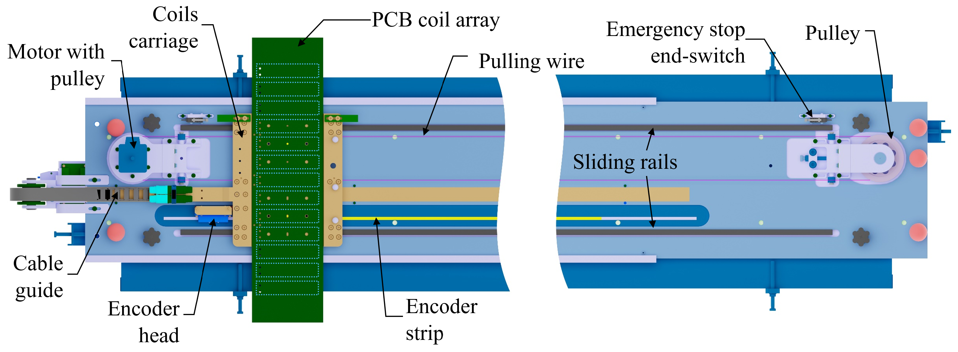
2. The Translating Fluxmeter Design
3. Calibration
3.1. Alignment
3.2. Coils Surface
3.3. Flux Offset
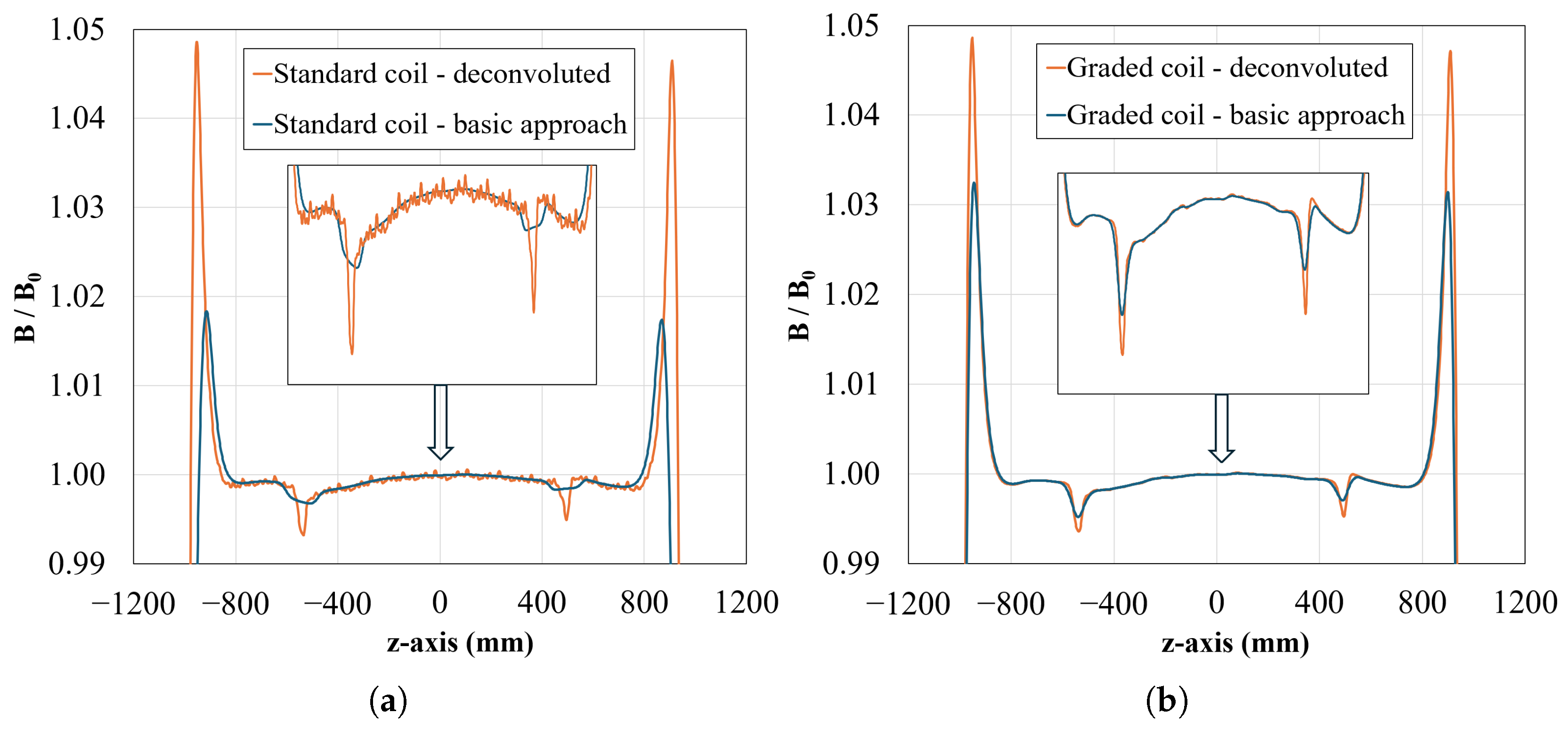
3.4. Convolution
4. Magnetic Field Measurement Applications
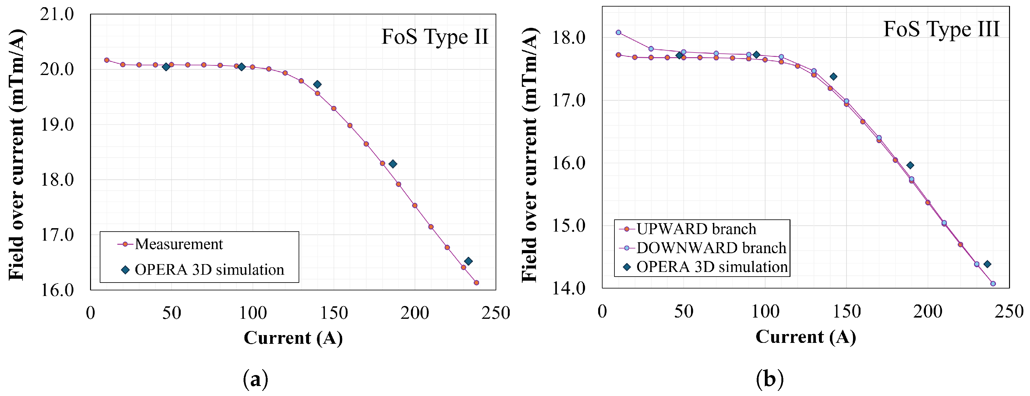
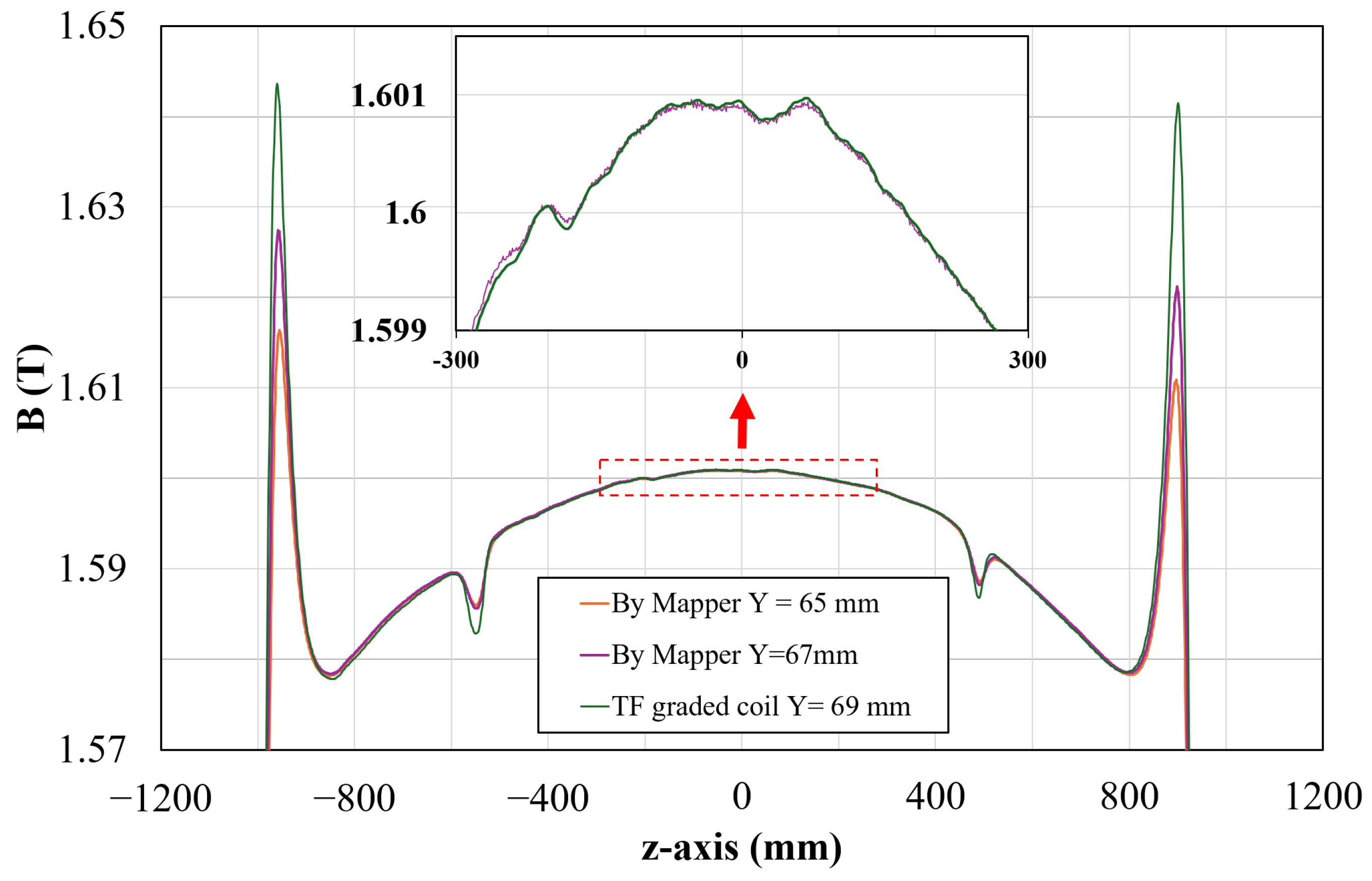
4.1. Main Field Loadline on Particle Trajectory
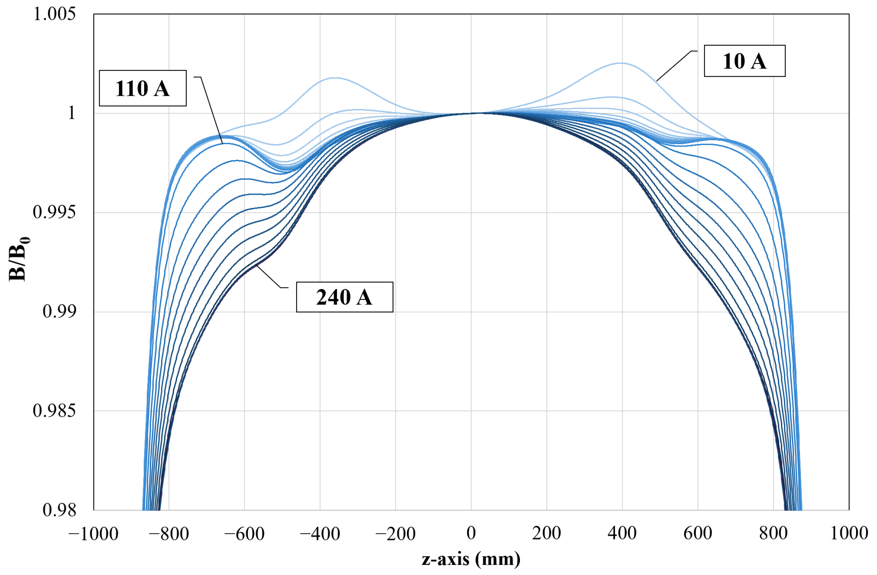
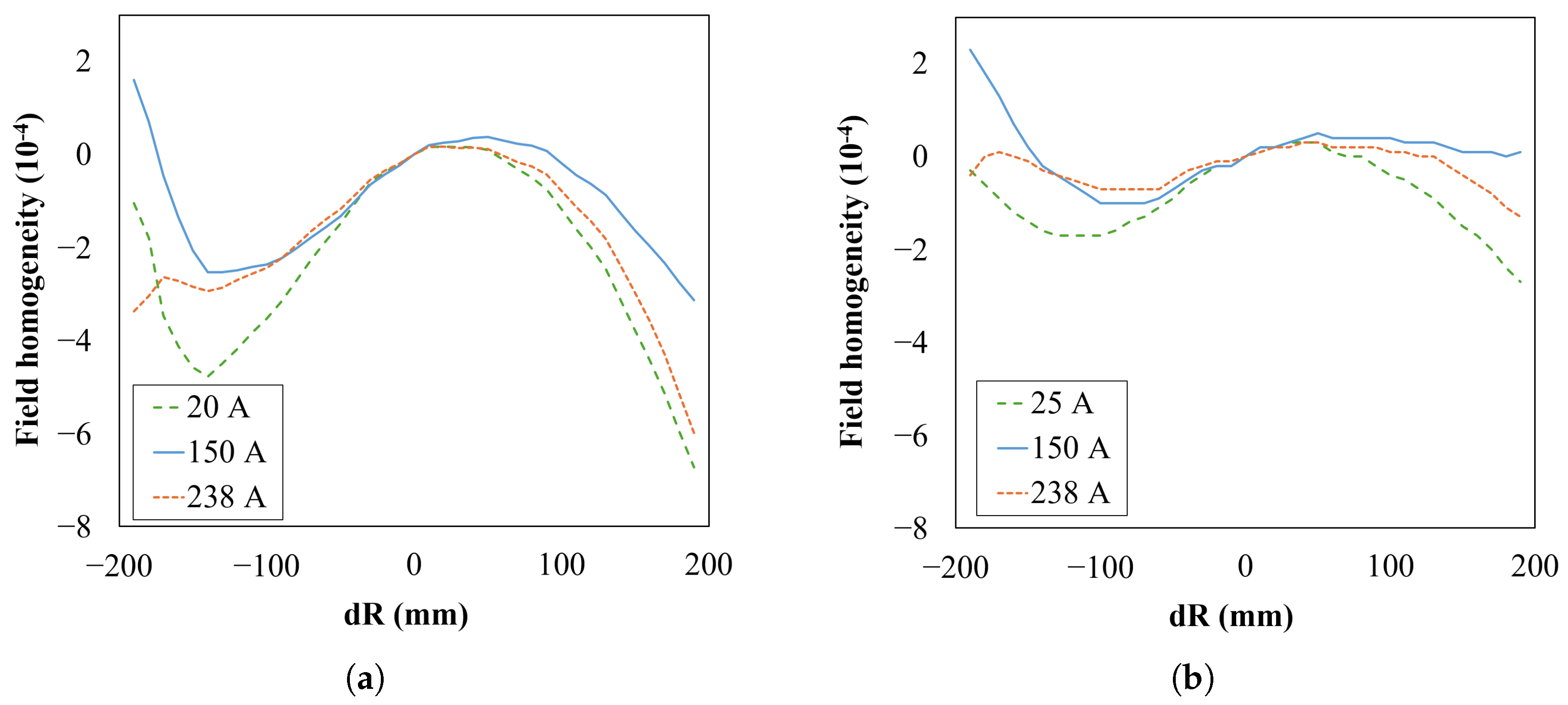
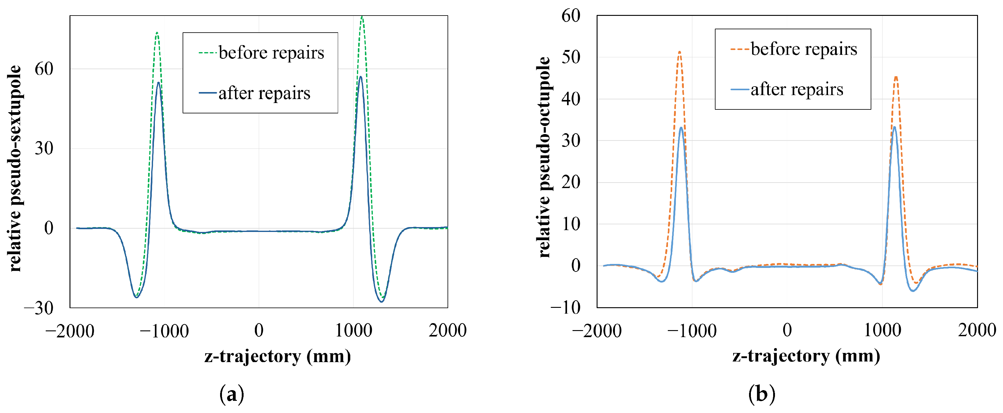
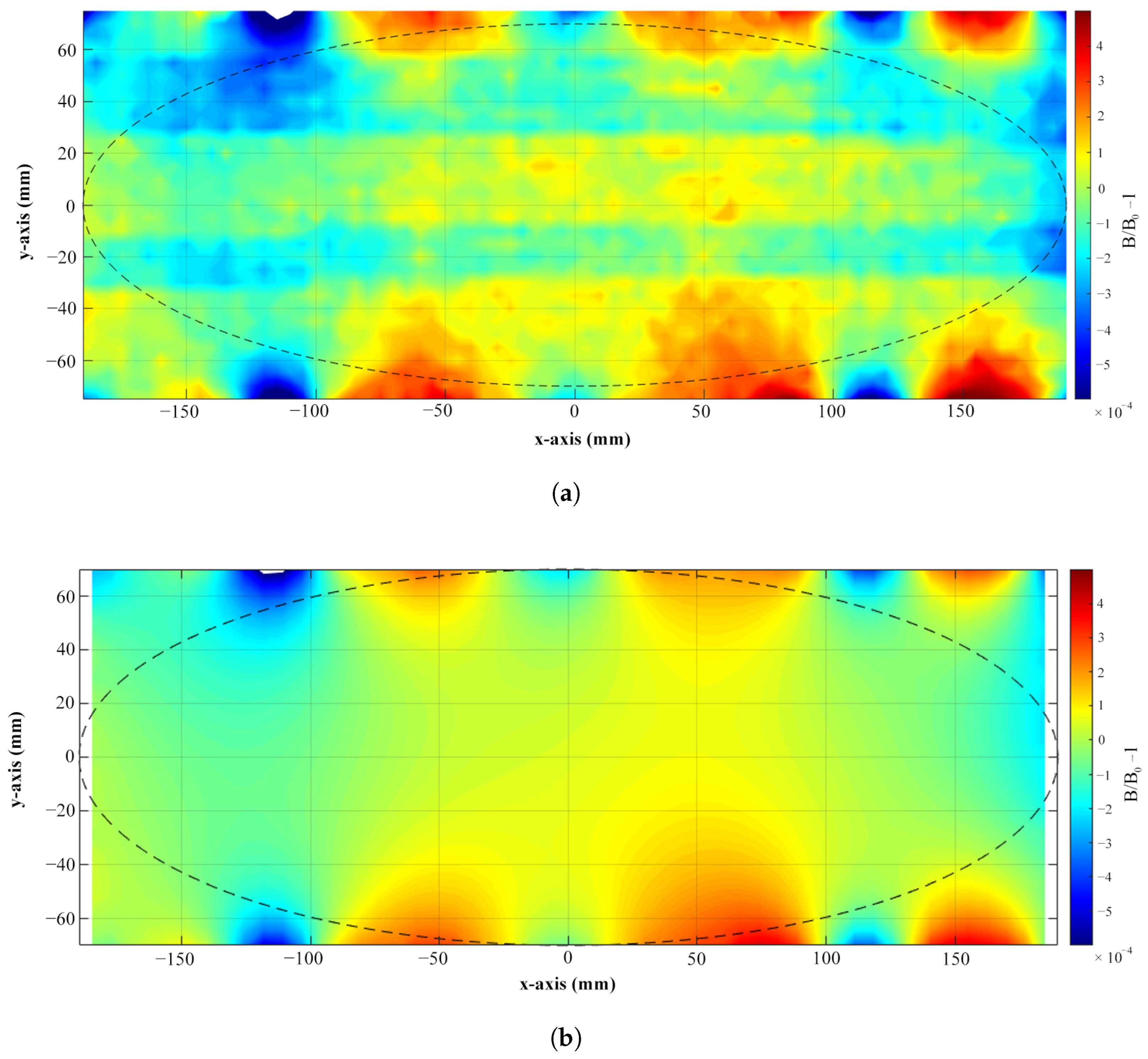
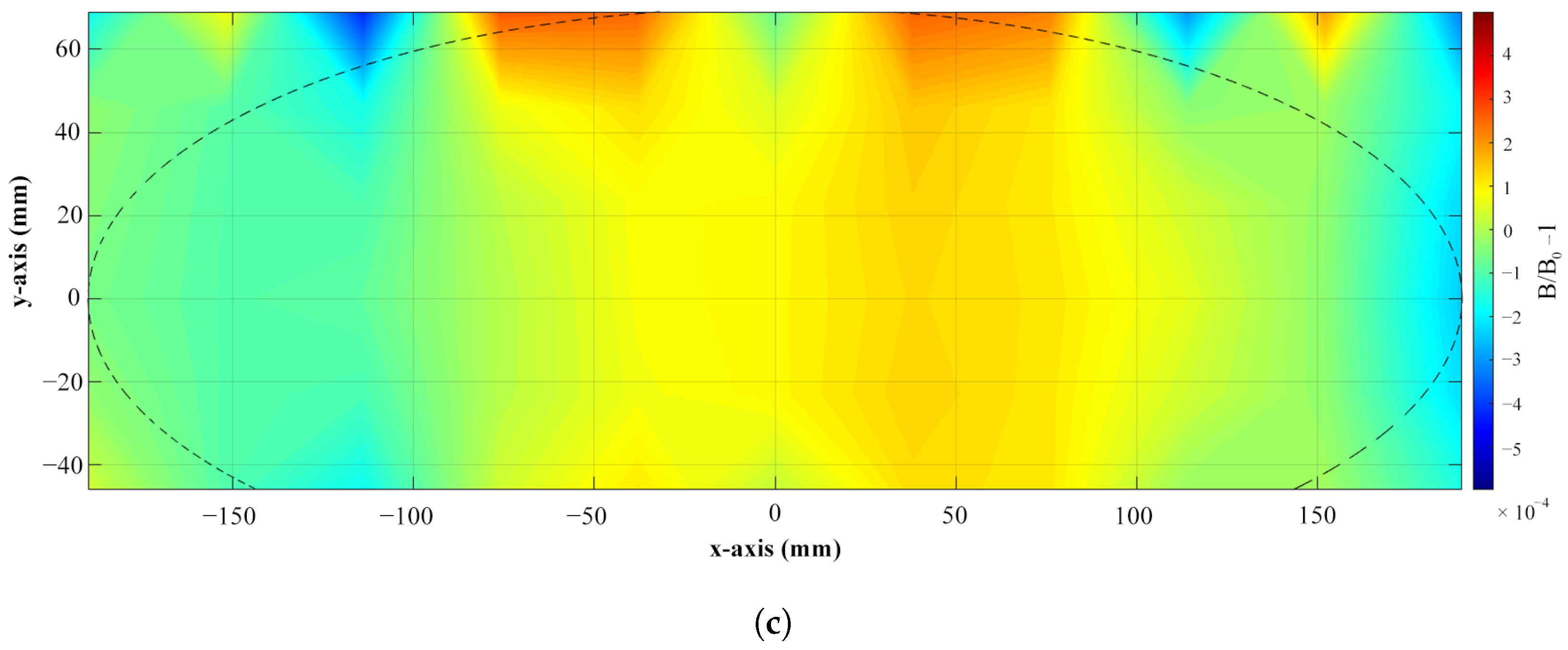
4.2. Field Quality
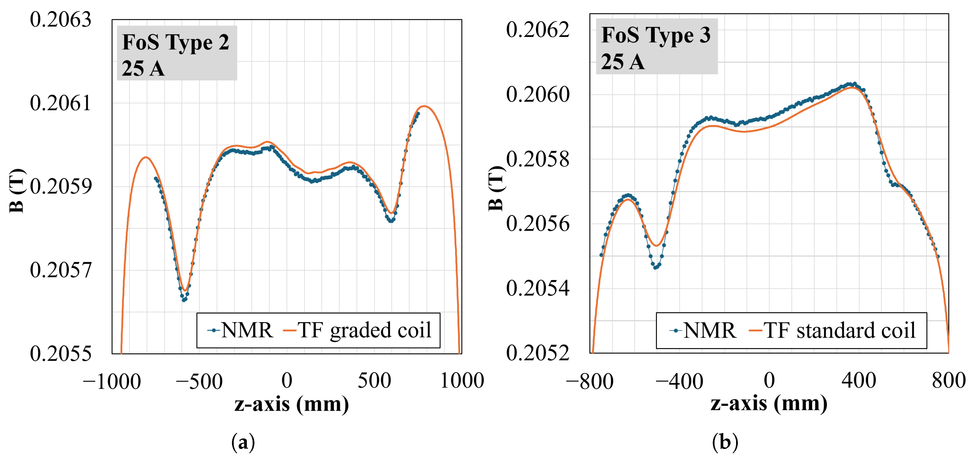
4.3. Local Field—Evaluation Against NMR
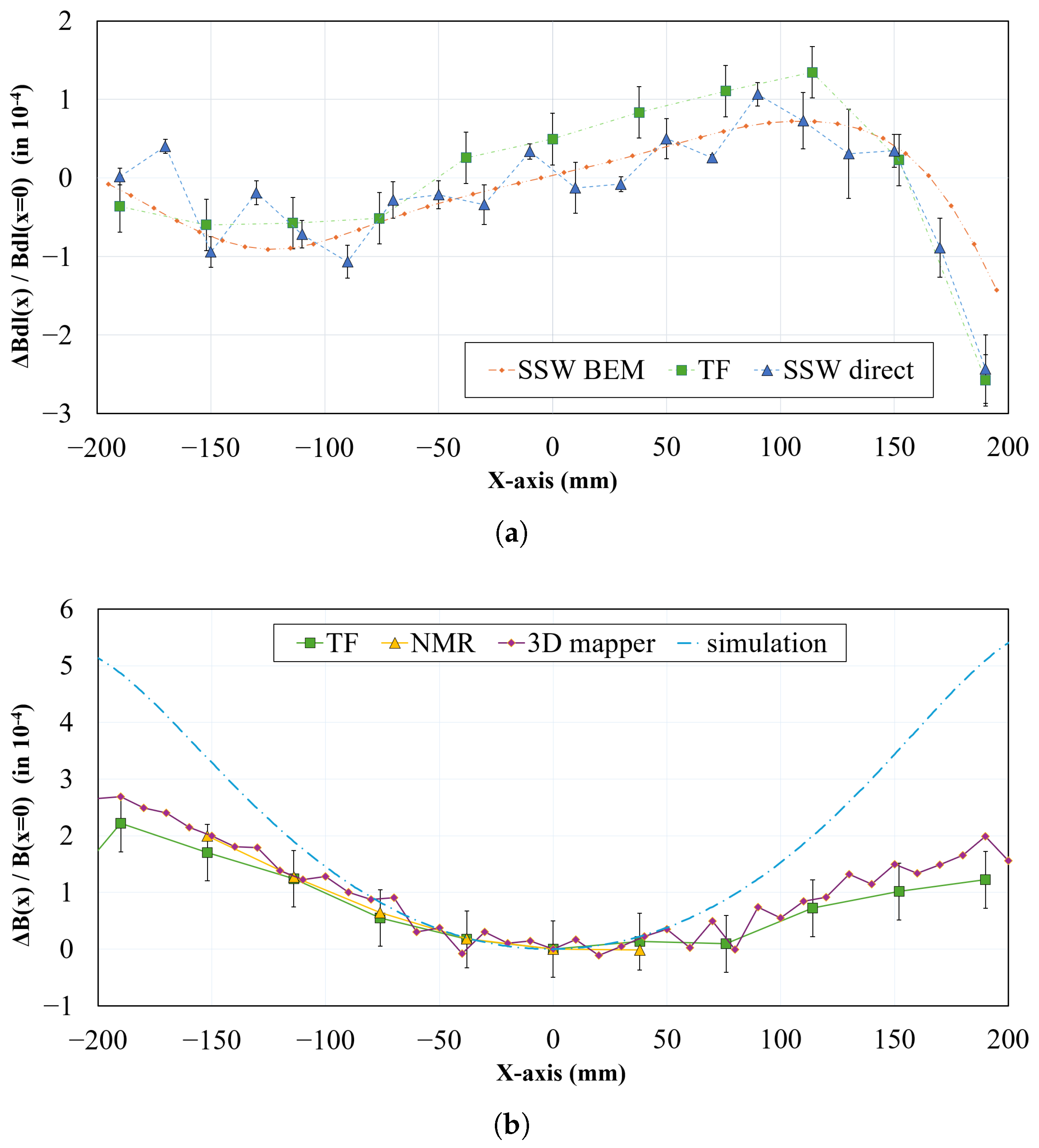
4.4. Integral Field—Evaluation Against Single Stretched Wire
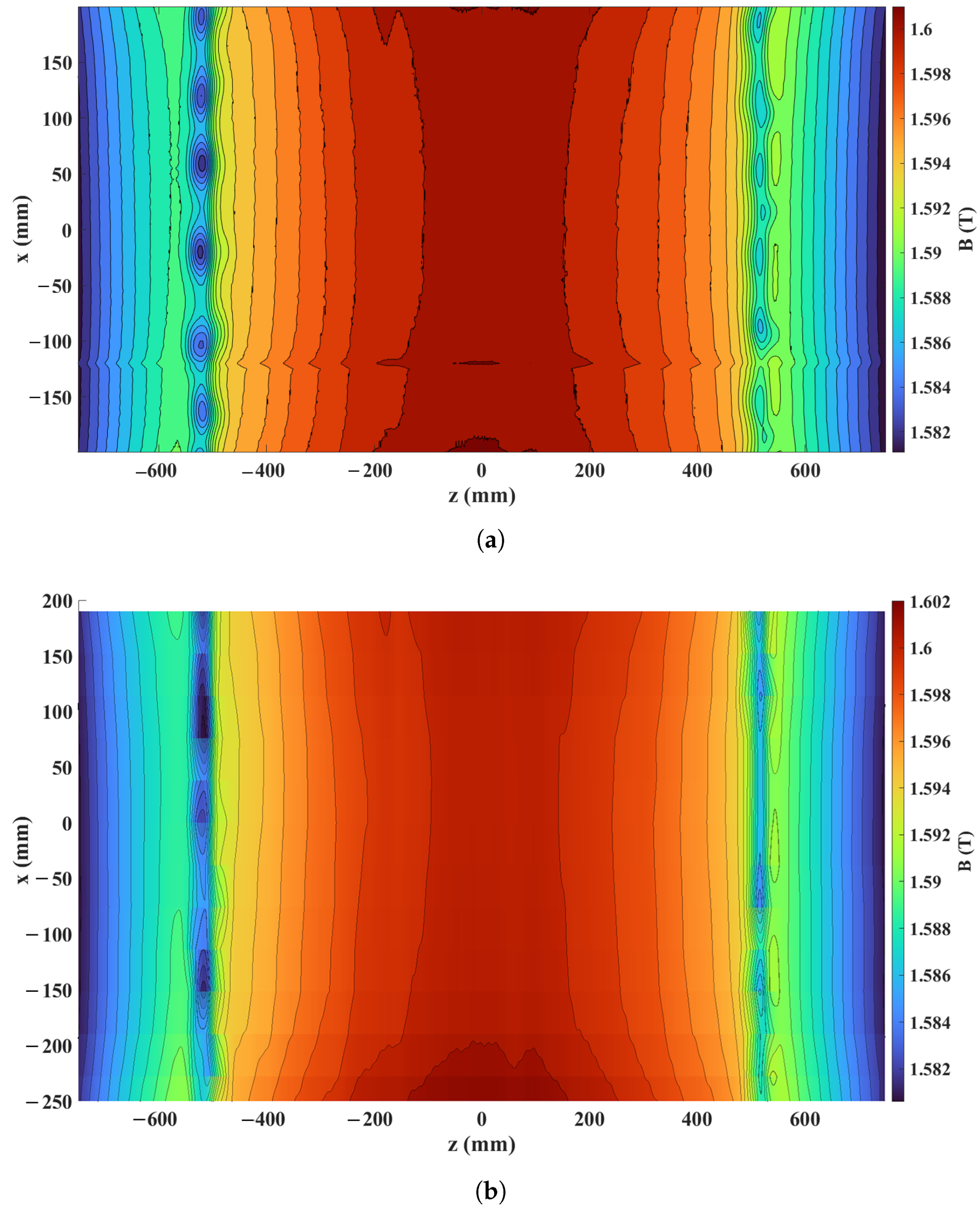
4.5. Field Map—Evaluation Against 3D Hall Probe Mapper
5. Conclusions
Author Contributions
Funding
Data Availability Statement
Acknowledgments
Conflicts of Interest
References
- FAIR—The Universe in the Lab. Available online: www.fair-center.eu (accessed on 1 August 2024).
- GSI—The Super-FRS Machine. Available online: https://www.gsi.de/work/gesamtprojektleitung_fair/super_frs/the_super_frs_machine (accessed on 23 February 2025).
- Geissel, H.; Weick, H.; Winkler, M.; Münzenberg, G.; Chichkine, V.; Yavor, M.; Aumann, T.; Behr, K.H.; Böhmer, M.; Brünle, A.; et al. The Super-FRS project at GSI. Nucl. Instrum. Methods Phys. Res. 2003, 204, 71–85. [Google Scholar] [CrossRef]
- Perin, A.; Derking, J.H.; Serio, L.; Stewart, L.; Benda, V.; Bremer, J.; Pirotte, O. A new cryogenic test facility for large superconducting devices at CERN. IOP Conf. Ser. Mater. Sci. Eng. 2015, 101, 012185. [Google Scholar] [CrossRef]
- Müller, H.; Fischer, E.S.; Leibrock, H.; Schnizer, P.; Winkler, M.; Munoz-Garcia, J.-E.; Quettier, L.; Serio, L. Status of the Super-FRS magnet development for FAIR. In Proceedings of the 6th International Particle Accelerator Conference, Richmond, VA, USA, 3–8 May 2015. [Google Scholar]
- Mueller, H.; Cho, E.; Michels, M.; Velonas, V.; Chiuchiolo, A.; Kosek, P.; Greiner, F.; Beaumont, A.; Sugita, K.; Winkler, M.; et al. Superconducting Dipoles for Super-FRS: Design, Production, First Measurements. IEEE Trans. Appl. Supercond. 2023, 33, 4004204. [Google Scholar] [CrossRef]
- Jain, A.K. Harmonic coils. In CAS—CERN Accelerator School: Measurement and Alignment of Accelerator and Detector Magnets; CERN: Geneva, Switzerland, 1998. [Google Scholar] [CrossRef]
- Petrone, C. Wire Methods for Measuring Field Harmonics, Gradients and Magnetic Axes in Accelerator Magnets. Ph.D. Thesis, University of Sannio, Benevento, Italy, 2013. [Google Scholar]
- Wallbank, J.V.; Buzio, M.; Parella, A.; Petrone, C.; Sammut, N. Pulsed-Mode Magnetic Field Measurements with a Single Stretched Wire System. Sensors 2024, 24, 4610. [Google Scholar] [CrossRef] [PubMed]
- Reymond, V. Magnetic resonance techniques. In CAS—CERN Accelerator School: Measurement and Alignment of Accelerator and Detector Magnets; CERN: Geneva, Switzerland, 1998; pp. 219–232. [Google Scholar] [CrossRef]
- Sanfilippo, S. Hall probes: Physics and application to magnetometry. In Proceedings of the CERN Accelerator School CAS 2009: Specialised Course, Magnets, Bruges, Belgium, 16–25 June 2009; CERN-2010-004. CERN: Geneva, Switzerland, 2010; pp. 423–462. [Google Scholar]
- Moritz, G.; Klos, F.; Langenbeck, B.; Youlun, Q.; Zweig, K. Measurements of the SIS magnets. IEEE Trans. Magn. 1988, 24, 942–945. [Google Scholar] [CrossRef]
- Priano, C.; Bazzano, G.; Bianculli, D.; Bressi, E.; Pullia, M.; Vuffray, L.; DeCesaris, I.; Buzio, M.; Cornuet, D.; Chritin, R.; et al. Magnetic modeling, measurements and sorting of the CNAO synchrotron dipoles and quadrupoles. In Proceedings of the IPAC 2010, Kyoto, Japan, 23–28 May 2010. [Google Scholar]
- Golluccio, G.; Buzio, M.; Caltabiano, D.; Deferne, G.; Dunkel, O.; Fiscarelli, L.; Giloteaux, D.; Petrone, C.; Russenschuck, S.; Schnizer, P. Instruments and methods for the magnetic measurement of the Super-FRS magnets. In Proceedings of the 7th International Particle Accelerator Conference, Busan, Republic of Korea, 8–13 May 2016. [Google Scholar]
- Arpaia, P.; Bottura, L.; Fiscarelli, L.; Walckiers, L. Performance of a fast digital integrator in on-field magnetic measurements for particle accelerators. Rev. Sci. Instrum. 2012, 83, 024702. [Google Scholar] [CrossRef] [PubMed]
- Liebsch, M.; Russenschuck, S.; Kaeske, J. An induction-coil magnetometer for mid-plane measurements in spectrometer magnets. Sens. Actuators Phys. 2023, 355, 114334. [Google Scholar] [CrossRef]
- Russenschuck, S. Field Simulations for Accelerator Magnets, 1st ed.; Wiley-VCH: Berlin, Germany, 2025. [Google Scholar]
- Liebsch, M. Inference of Boundary Data from Magnetic Measurements of Accelerator Magnets. Ph.D. Thesis, Technische Universität Darmstadt, Darmstadt, Germany, 2022. [Google Scholar]
- Bottura, L.; Henrichsen, K.N. Field Measurements. In CAS—CERN Accelerator School: Superconductivity and Cryogenics for Accelerators and Detectors; CERN: Geneva, Switzerland, 2004; pp. 118–148. [Google Scholar] [CrossRef]
- Russenschuck, S.; Caiafa, G.; Fiscarelli, L.; Liebsch, M.; Petrone, C.; Rogacki, P. Challenges in extracting pseudo-multipoles from magnetic measurements. In Proceedings of the 13th International Computational Accelerator Physics Conference, Key West, FL, USA, 20–24 October 2018. [Google Scholar]
- Liebsch, M.; Russenschuck, S.; Kurz, S. Boundary-Element Methods for Field Reconstruction in Accelerator Magnets. IEEE Trans. Magn. 2022, 56, 7511104. [Google Scholar] [CrossRef]
- Caltabiano, D. Design and Development of a Translating-Coil Magnetometer. Master’s Thesis, University of Modena and Reggio Emilia, Modena, Italy, 2016. [Google Scholar]
- Windischhofer, A. Metrological Characterization of a Translating-Coil Magnetometer for Measuring the Field Quality in Dipole Magnets. Master’s Thesis, Technische Universität Wien, Vienna, Austria, 2022. [Google Scholar]

| Unit | Dipole Type II | Dipole Type III | |
|---|---|---|---|
| Number of magnets | - | 3 | 21 |
| Weight | kg | 61,300 | 54,100 |
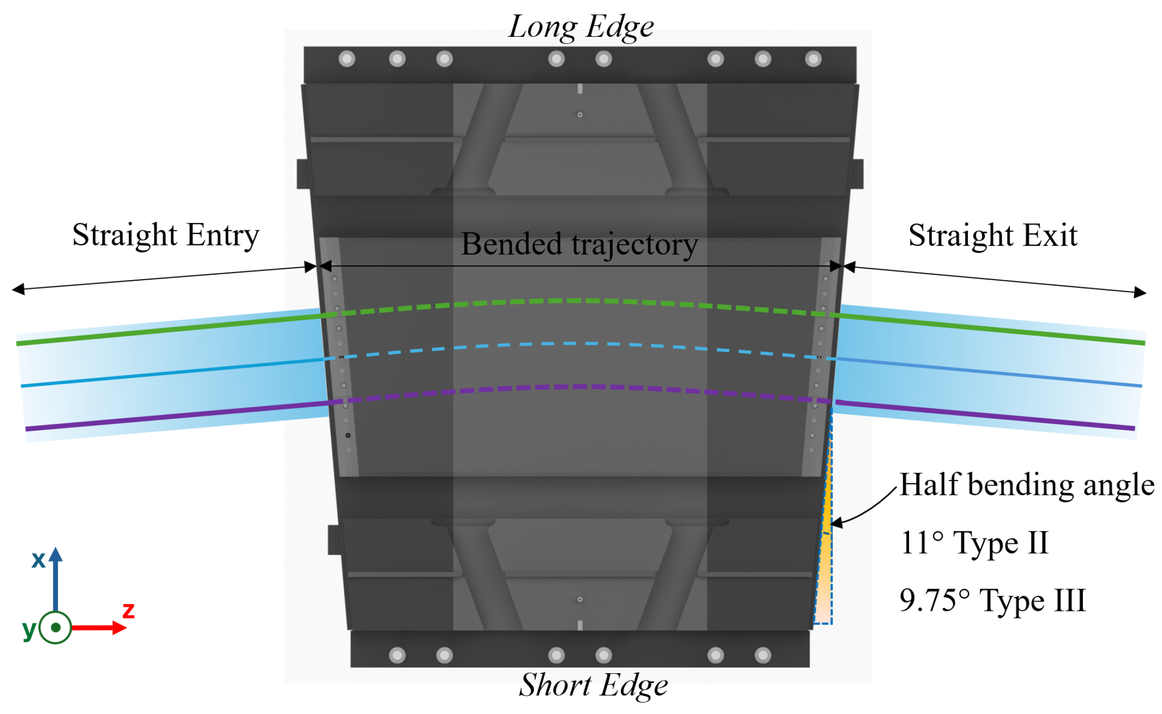
| Bending angle | ° | 11 | 9.75 |
| Curvature radius | m | 12.5 | |
| Coil layers/turns | - | 28/20 | |
| Coil Ampere-turn (for 233 A) | A | 260,960 | |
| Inductance | H | 18.2 | 15.8 |
| Magnetic Stored Energy | kJ | 651.9 | 591.6 |
| Nominal central field | T | 1.6 | |
| Nominal integral field | Tm | 3.84 | 3.40 |
| Good field region semi-major axis/semi-minor axis | mm | 190/70 | |
| Aperture | mm | 170 | |
| Integral field quality | - | ||
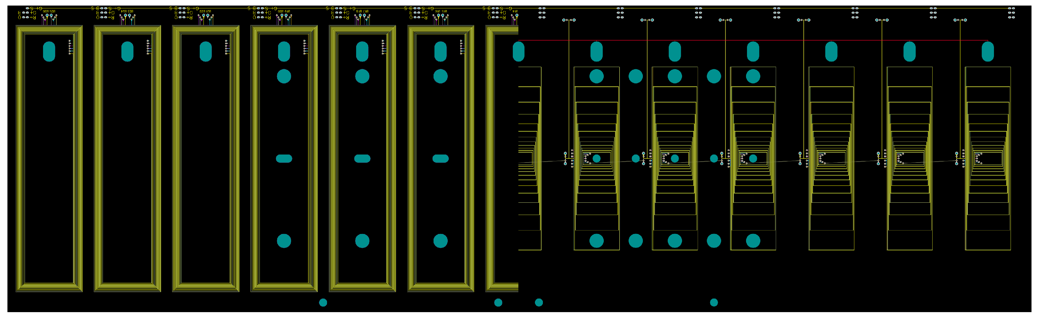
| Unit | Rectangular Coils | Graded Coils | |
|---|---|---|---|
| Board width | mm | 500 | |
| Board length | mm | 150 | |
| Number of coils | - | 13 | |
| Coils spacing | mm | 38 | |
| Coil inner length | mm | 120.9 | 6.13 |
| Coil inner width | mm | 23.6 | 13.4 |
| Number of layers | - | 12 | 14 |
| Number of coil turns per layer | - | 12 | |
| Nominal coil area | m2 | 0.486 | 0.1085 |
| Translating Fluxmeter | NMR | SSW | 3D Hall Probe Mapper | Static Fluxmeter | |
|---|---|---|---|---|---|
| Magnet powering mode | DC | DC | DC/AC | DC | AC |
| Local/integral field | Local and Integral | Local | Integral on a straight line | Local | Integral |
| Measurement speed | Fast | Very Slow | Slow | Slow | Fast |
| Measured field component | and | ||||
| Horizontal/vertical resolution | 38 mm/24 mm semi-flexible | up to 1 mm (NMR mapper) | ∼5 mm (for usable signal strength in moderate field) | Unlimited | Typically few tens of mm |
| Longitudinal resolution | 0.16 mm | up to 1 mm (NMR mapper) | None | Unlimited | None |
| Absolute measurement accuracy | 100 ppm (needs calibration) | up to 1 ppm | ∼100 ppm | up to 100 ppm (needs calibration) | up to 10 ppm (needs calibration) |
Disclaimer/Publisher’s Note: The statements, opinions and data contained in all publications are solely those of the individual author(s) and contributor(s) and not of MDPI and/or the editor(s). MDPI and/or the editor(s) disclaim responsibility for any injury to people or property resulting from any ideas, methods, instructions or products referred to in the content. |
© 2025 by the authors. Licensee MDPI, Basel, Switzerland. This article is an open access article distributed under the terms and conditions of the Creative Commons Attribution (CC BY) license (https://creativecommons.org/licenses/by/4.0/).
Share and Cite
Kosek, P.; Beaumont, A.; Liebsch, M. Assessment of a Translating Fluxmeter for Precision Measurements of Super-FRS Dipole Magnets. Metrology 2025, 5, 37. https://doi.org/10.3390/metrology5020037
Kosek P, Beaumont A, Liebsch M. Assessment of a Translating Fluxmeter for Precision Measurements of Super-FRS Dipole Magnets. Metrology. 2025; 5(2):37. https://doi.org/10.3390/metrology5020037
Chicago/Turabian StyleKosek, Pawel, Anthony Beaumont, and Melvin Liebsch. 2025. "Assessment of a Translating Fluxmeter for Precision Measurements of Super-FRS Dipole Magnets" Metrology 5, no. 2: 37. https://doi.org/10.3390/metrology5020037
APA StyleKosek, P., Beaumont, A., & Liebsch, M. (2025). Assessment of a Translating Fluxmeter for Precision Measurements of Super-FRS Dipole Magnets. Metrology, 5(2), 37. https://doi.org/10.3390/metrology5020037