Comparison of Magnetic Field Maps by Direct Measurement and Reconstruction Using Boundary Element Methods

Abstract

Boundary Element Methods (BEMs) can be applied to determine the value of the magnetic field at any point within a domain if the magnetic field components are measured on the surface of the domain. For large magnetic volumes, BEMs provide an attractive alternative to fine three-dimensional Hall probe scans for determining the local shape of the field as the fields can be evaluated inside the volume with an arbitrary position and with a reduced measurement time. BEMs have been applied to the field data measured on the boundary of three-dimensional Hall probe scans for two example magnets, which have been measured at STFC Daresbury Laboratory, UK. The fields reconstructed using BEMs are compared to the fields directly measured during the Hall probe scans. The reconstructed fields can be calculated to within 1 mT rms of the directly measured fields. For the transverse field components greater than 1 mT, the fields can be reconstructed to within 5% rms of the directly measured fields.

1. Introduction

Magnets are used in particle accelerators to bend and focus particle beams. The field quality of an accelerator magnet describes the differences between the actual field of a built magnet and the desired field. Accurate measurement of the magnetic field inside accelerator magnets is crucial for determining the errors in the magnetic field and ensuring these are within acceptable limits as set by the physics requirements [1]. The impact on the beam can be determined through particle tracking simulations using the measured fields [2].

The most common method for expressing magnetic field measurements is as eigenfunctions of the Laplace equation in polar coordinates. These eigenfunctions are often referred to as field harmonics [1,3]. Expression as field harmonics has many advantages. Particularly, the harmonics form a magneto-static solution which obeys Maxwell’s equations, allowing fields within a measurement radius to be reconstructed [2].

The evaluation of two-dimension field harmonics is well known for use with beam dynamics calculations [4,5]. Stretched wire [6,7] and rotating coil magnetometer [8,9,10] measurements can be performed to efficiently measure the integrated field harmonics of accelerator magnets. Stretched wire measurement benches have great utility, allowing quick and highly accurate cylindrical harmonic measurements of variable measurement radii and variable axial lengths. Specialised rotating coil sensors can be built for the accurate measurement of specified field harmonics, even under the influence of mechanical perturbations [11]. More complex measurements using stretched wires can also be used to compensate some multipole components for more accurate measurements of field errors [6]. The use of field harmonics for particle tracking codes is well established. The generalised gradient technique can be used to approximate the fringe fields of a magnet based on measurements of the radial field components on a reference radius [12,13]. However, these techniques are subject to errors due to the high order derivatives that are required to accurately model the fringe fields [12].

However, integrated field measurements using wires or magnetometers cannot be used to evaluate the local behaviour of the field along curved trajectories [14] or other arbitrary reference trajectories in radiotherapy beamlines, mass spectrometers and detector magnets [2].

Hall sensors are the standard for accurately measuring the direction and magnitude of flux density at a point. The magnetic field within a volume can be mapped using a series of point-by-point measurements using a Hall sensor to give information about the local field shape [15,16,17]. However, the time required to measure the fields inside a volume is directly dependent on the number of measured points and the travel time between them. As the volume dimensions increase, the choice must be made between an increasingly granular measurement or allowing the measurement time to increase. Therefore, high detail point-by-point measurements of large magnets take extremely long times to be performed, with accuracy then dependent on the long-term stability and temperature control of the measurement area.

Boundary element methods (BEMs) provide an alternative method for evaluating the magnitude and direction of the magnetic flux density at any point within the measurement volume [18]. BEMs only require knowledge of the magnetic field on the surface of the measurement volume. Therefore, the number of points that need to be evaluated scales on the order of the square of the volume dimensions rather than on the cube of those dimensions, and hence the time required to fully characterise the magnetic field within a large volume can be significantly reduced.

A further advantage of the BEM is that it can be used to evaluate the fields within arbitrarily shaped volumes. A two-dimensional BEM has been used to evaluate the integrated fields within racetrack volumes for dipole and undulator magnets, which have large aspect ratios and cannot be efficiently described using circular or elliptical multipoles [19,20]. Three-dimensional multipoles provide an alternative method for determining the field vectors, including fringe fields and longitudinal fields over a volume. However, these methods are restricted to spherical or cylindrical volumes [21]. BEMs can be used to evaluate fields within curved volumes for the measurement of long dipole magnets [2] and cuboid volumes with large aspect ratios for the measurement of dipoles and undulators [21].

A method of using a BEM to reconstruct the magnetic fields based on the measurements of magnetic flux densities on the boundary of a cuboid volume using a 3-axis Hall sensor has been developed. The boundary data have been extracted from three-dimensional grids of field measurements for two magnets which have been previously measured before installation in their respective facilities. The reconstructed fields have been compared to those measured directly using the Hall sensor within the grid. This method allows a direct comparison of the magnitude and direction of field vectors measured at a point by a direct Hall sensor measurement and by using the BEM.

2. Materials and Methods

The magnetic flux density B in an open domain $\mathrm{\Omega }$ which is free of currents and magnetic materials can be described in terms of the permeability of free space ${\mu }_0$ and the magnetic scalar potential ${\varphi }_m$ [3]:

$$\mathbf{B}=-{\mu }_0\nabla {\varphi }_m$$

(1)

As the divergence of the magnetic flux density is zero, the magnetic scalar potential forms a solution to Laplace’s equation [22]:

$$▵{\varphi }_m=0$$

(2)

Therefore, the representation formula for the Laplace equation can be used to reconstruct the magnetic scalar potential at any point inside the domain $\mathrm{\Omega }$ [23]:

$${\varphi }_m\left(\mathbf{r}\right)=\left(\tilde{V}{\delta }_n{\varphi }_m\right)\left(\mathbf{r}\right)-\left(W{\varphi }_m\right)\left(\mathbf{r}\right)$$

(3)

where $\tilde{V}$ and $\mathit{W}$ are the single layer and double layer potential operators, respectively, and ${\delta }_n{\varphi }_m$ is the normal derivative of the magnetic scalar potential on the domain boundary.

The magnetic scalar potential on the domain boundary and its derivative normal to the boundary are referred to as the Dirichlet data $\mathit{u}$ and Neumann data ${\mathit{g}}_{\mathit{N}}$, respectively, in the context of BEMs [20]. If both the Dirichlet and Neumann data are known, the representation formula can be used to evaluate the magnetic scalar potential and hence the magnetic flux density at any point within the domain.

The Neumann data on the domain boundary are directly proportional to the magnetic flux density vector normal to the boundary, as shown in Equation (1). Therefore, the Neumann data can be directly computed from measurements of the flux density on the domain boundary using a 3-axis Hall sensor.

With the Neumann data known, the Dirichlet data can be computed using a Neumann to Dirichlet map [18]:

$$Du=({\displaystyle \frac{1}{2}}Id-K^{\prime })g_N$$

(4)

where D, Id and K′ are the hypersingular, identity and adjoint double layer potential boundary operators, respectively [23].

Therefore, if the magnetic flux density vectors are measured directly on the domain boundary using a 3-axis Hall sensor, the Neumann and Dirichlet data can be evaluated, the magnetic scalar potential reconstructed inside the domain and the potential differentiated to calculate the magnetic flux density vectors at any point within the domain.

The accuracy of using BEMs to reconstruct magnetic flux density field maps inside measurement domains has been evaluated by comparing the fields reconstructed using the BEM with fields directly measured on 3D grids using a 3-axis Hall sensor. Measurements have been performed using a Senis Type C 3-axis Hall sensor and a 3MH6 Teslameter [24] to calculate the flux density vectors at a set of discrete, regularly spaced points within cuboid measurement domains inside two test magnets. The type C probe contains 3 individual sensors and so can measure the three orthogonal field components simultaneously. The spacial resolution of the probe, as stated by the manufacturer, is 30 × 5 × 30 μm³ for the $B_y$ field component and 100 × 10 × 100 μm³ for the $B_x$ and $B_z$ field components. The planar Hall effect is suppressed through the application of the spinning current technique. The 3MH6 Teslameter provides an accuracy of 0.01% and a precision of 1 μT. The sensor has been translated in the grid using a precision 3-axis motion system. The probe was mounted in a custom-designed 3D-printed holder. This holder was bolted to an extruded aluminium arm, which was connected to the motion stages. An image of this arrangement is shown in Figure 1. This motion system achieves 5 μm precision in the transverse (x) and vertical (y) planes and 10 μm precision in the axial plane (z) through the use of stepper motors and absolute encoders. The achieved precisions are defined by an allowable tolerance set in the motion control software between the set and measured absolute position of the stages. The software polls the read position of the stages after sending a movement command. If the read position is not within the given precision set by the tolerance within a set time, a time-out error is raised. The set precisions have been found to be practical limits which allow large 3D scans to be performed without time-out errors being regularly raised. A granite bench provided vibration isolation to the probe. The magnets were supported on their own frames, independent of the granite bench. The Hall sensor was connected to the Teslameter through a CaH cable. The fields measured by the Teslameter were recorded by the control PC through a USB connection. Every point measurement of the field was recorded as an average of 1000 samples recorded at a sample rate of 1 kHz. The results between the fields at the directly measured points within the domain grid and the fields reconstructed from the boundary data only were compared to assess the accuracy of the BEM-reconstructed fields.

All of the BEM calculations have been performed using the Boundary Element Method Python Package (Bempp) version 0.3.1 [25] in Python version 3.11.7, an open-source Python package for solving three-dimensional boundary element problems. The package includes pre-built definitions of the required potentials and boundary operators for solving the Laplace boundary integral equations with Neumann boundary conditions. The package also supports the generation of the triangular mesh used to evaluate the Neumann and Dirichlet data on the boundary of a set of standard grid shapes through the meshio library. The current version of Bempp only supports the generation of triangular surface meshing. Custom triangular meshes can be defined for arbitrary shaped volumes. The restriction to triangular meshes is specific to the software package used and is not a limitation of the BEM in general, which can use other mesh shapes. For all of the measured 3D grids, the Neumann data on the BEM mesh have been approximated by fitting a cubic radial basis function to the field components measured normal to each face on the measurement volume. The calculations were performed using a PC with AMD Ryzen 9 7900 X3D 12-core processor, 64 GB physical memory and solid state drive with 1.81 TB available memory. The package Bempp also supports GPU acceleration through OpenCL; however, this was not exploited in this work.

3. ZEPTO-Q3 Quadrupole

The Zero-Power Tuneable Optics (ZEPTO) project aims to produce permanent magnets as energy saving alternatives to standard electromagnets in particle accelerators [26]. These magnets employ permanent magnet blocks as the source of the magnetic field, as opposed to resistive copper coils. Unlike standard permanent magnets, the ZEPTO magnets utilise the mechanical movement of the permanent magnet blocks relative to fixed steel poles to tune the strength of the field in the magnet bore. The ZEPTO-Q3 quadrupole is the third quadrupole built based on the ZEPTO technology [27,28]. This quadrupole was built as a demonstrator of ZEPTO technology on a working accelerator facility. ZEPTO-Q3 was successfully installed and tested on the Diamond Light Source (DLS) Booster-to-Synchrotron line in August 2022 [29].

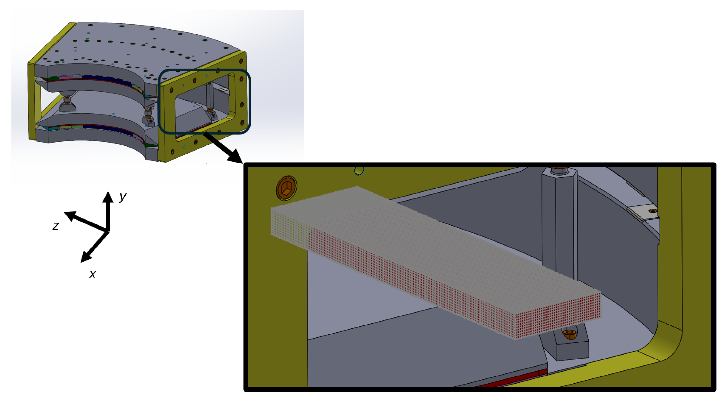
Before installation at the DLS, the ZEPTO-Q3 underwent extensive magnetic measurements to verify the field gradient and homogeneity in order to understand the focussing and higher-order impacts on the beam that would be introduced by the quadrupole. One of the measurements performed was a point-by-point scan over a 3D grid whilst the magnet was set to its highest gradient strength configuration. The measured volume extended from outside the magnet into a point part way through the magnet bore. The Hall probe mounting system prevented measurements being conducted along the whole length of the bore. The grid spanned a volume of 6 × 6 × 190 mm³. The points were separated by 1 mm in the transverse (x) and vertical (y) dimensions and 5 mm in the longitudinal (z) direction. The grid contained a total of 1911 individual points and took an hour for the measurement to be completed. By contrast, there were only 738 points on the boundary of the grid. Therefore, a measurement of points just on the boundary would have taken only 25 min to complete. The finite element software Opera [30] was used for the magnetic modelling of the ZEPTO-Q3. Figure 2 shows an image of the model of the quadrupole, with the grid of measurement points shown by the red points. The coordinate system shown in the image is orthogonal to the motion controller coordinate system used for the measurements. However, the origin of the measurements was not coincident with the centre of the magnet.

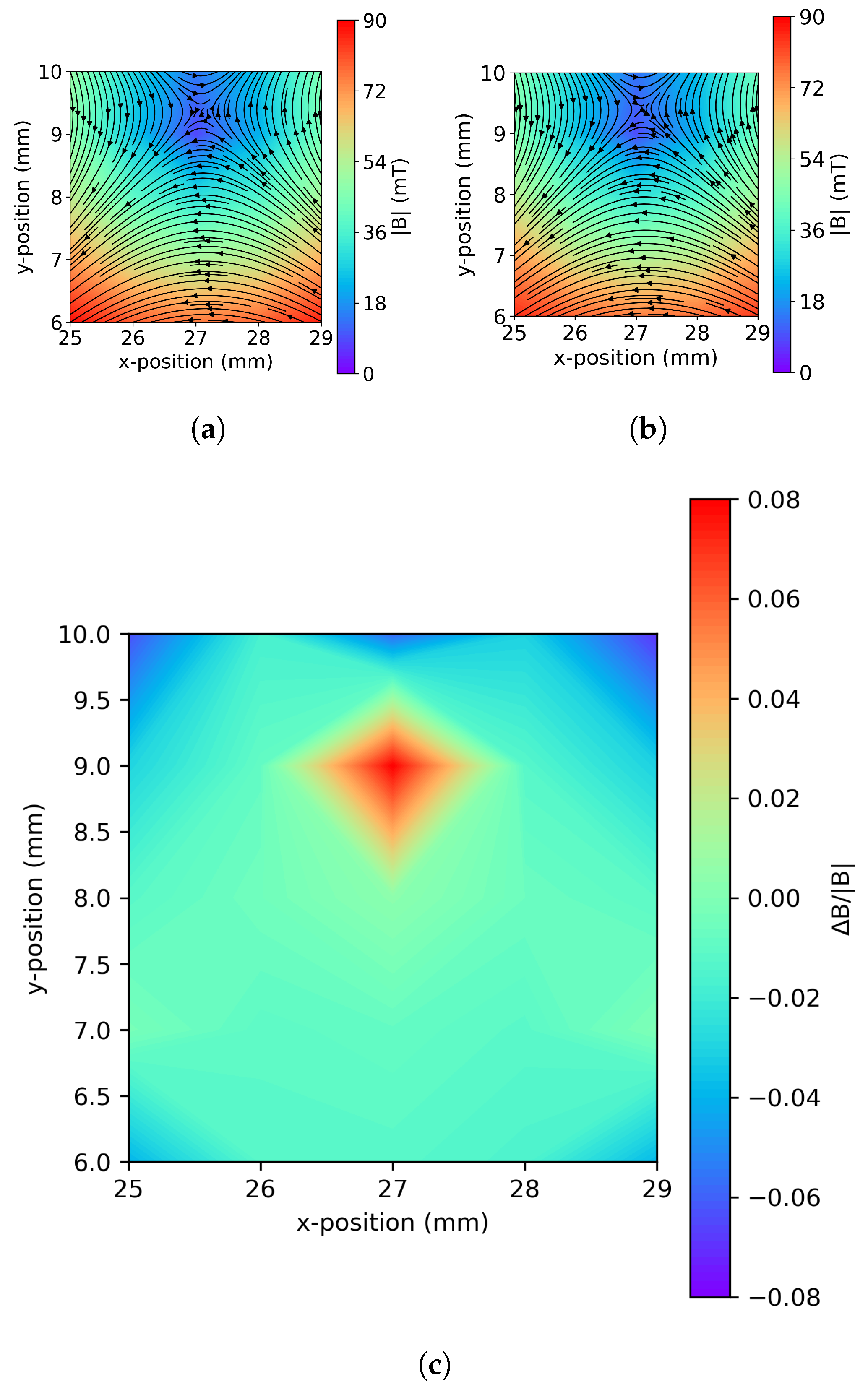
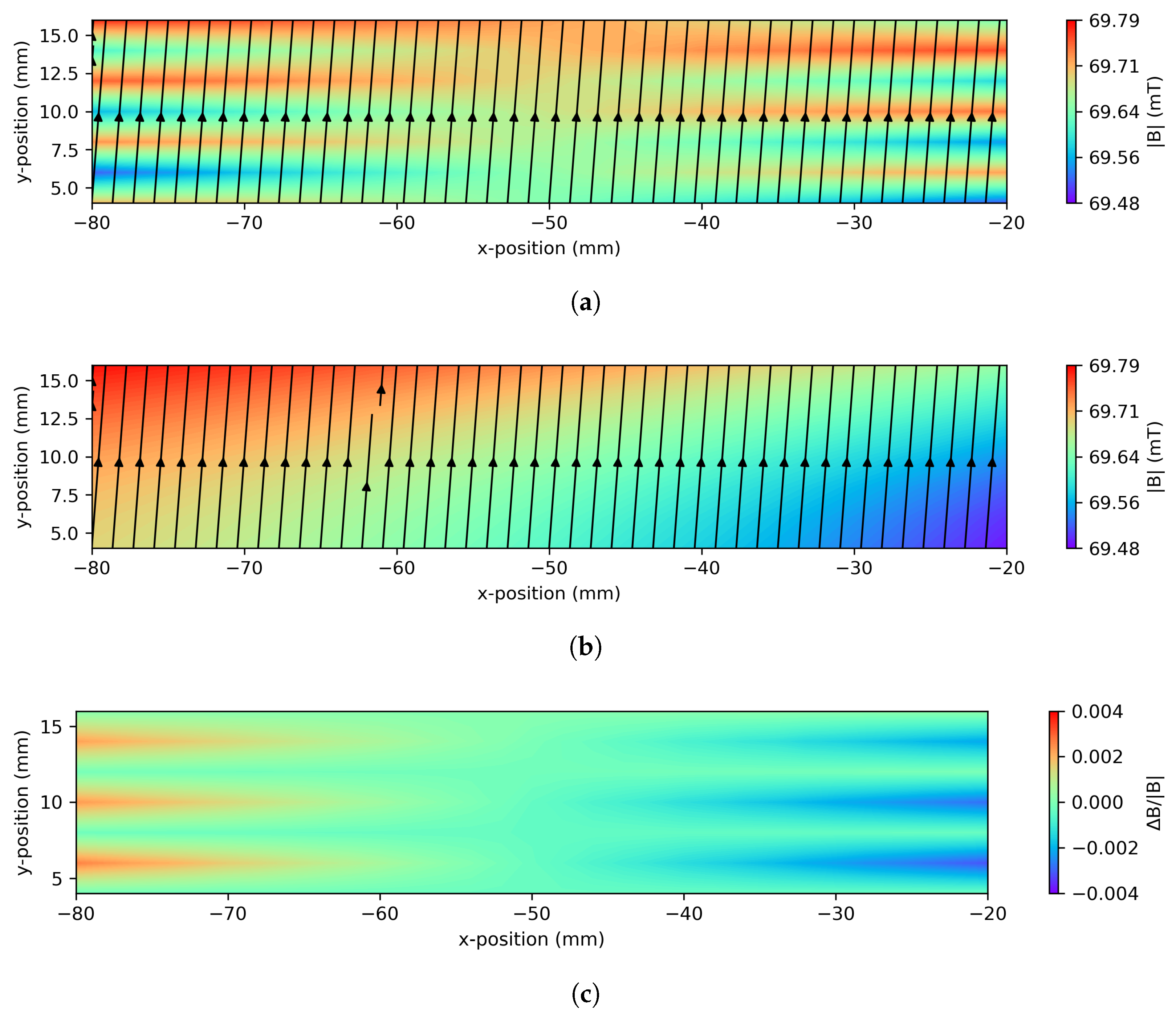
Figure 3 shows contour plots showing the magnitude and local direction of the magnetic field vectors in the xy plane at a fixed z-axis coordinate inside the magnet bore (z = 80 mm in the motor controller reference frame). Figure 3a shows the contour plot generated from the fields directly measured on the 3D grid. The plot shows the general shape expected for a quadrupole magnet, with the magnetic centre close to the point x = 27 mm, y = 9 mm. Figure 3b shows the field contours over the same plane for fields reconstructed using the BEM based on the field measurements on the boundary of the grid only. A 1 mm mesh size was used for the BEM calculations. It can be seen that this plot is in good agreement with the directly measured fields. The BEM fields show the same general shape and magnitude as the direct measurements. Figure 3c shows the relative difference in field magnitude ($\Delta$B/|B|) between the directly measured and BEM fields. The differences are low, in the range of −8 to +8 %. The largest relative differences are in the corners of the plane, close to the boundary of the measured volume, and near the magnetic centre. At the magnetic centre, the absolute measured fields go to zero, so small differences in the measured and reconstructed fields result in large relative errors.

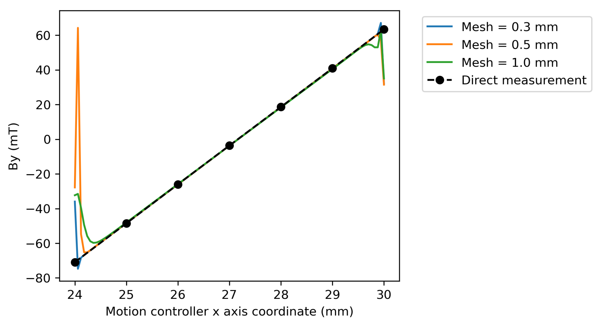
It is at the points closest to the measurement boundary that the BEM integral equations break down and the agreement between the directly measured and BEM fields becomes worse. Figure 4 shows a plot of the $B_y$ field component plotted against the motor controller x-axis in the plane y = 8 mm, z = 65 mm. The different coloured lines represent the BEM fields calculated using different mesh sizes and the black dashed line is a guide to the eye connecting the points showing the fields measured directly on the 3D grid. There is visually very good agreement between the BEM and directly measured fields between x coordinates of 25 mm and 29 mm. Towards the edges of the domain (x = 24 mm and 30 mm), the agreement breaks down and there are pronounced deviations between the BEM and directly measured field components. It can be seen that these deviations occur closer to the boundary for smaller mesh sizes. It is apparent from the shape of these deviations that the BEM fields calculated near the boundary are not good representations of the actual field. As a general rule, fields calculated using the BEM near the centre of the volume can be considered to be more accurate than those calculated near the boundary. Therefore, the boundary must extend further than the actual region of interest. It is good practice for the boundary to exceed the region of interest by at least one mesh size in all directions. The requirement to use BEM results at a distance of greater than one mesh size from the boundary has been observed in other works on reconstructing particle accelerator magnetic fields [20]. This behaviour can be explained by the divergence of the boundary integral equations at the boundaries due to the singularity of the Green’s function [31].

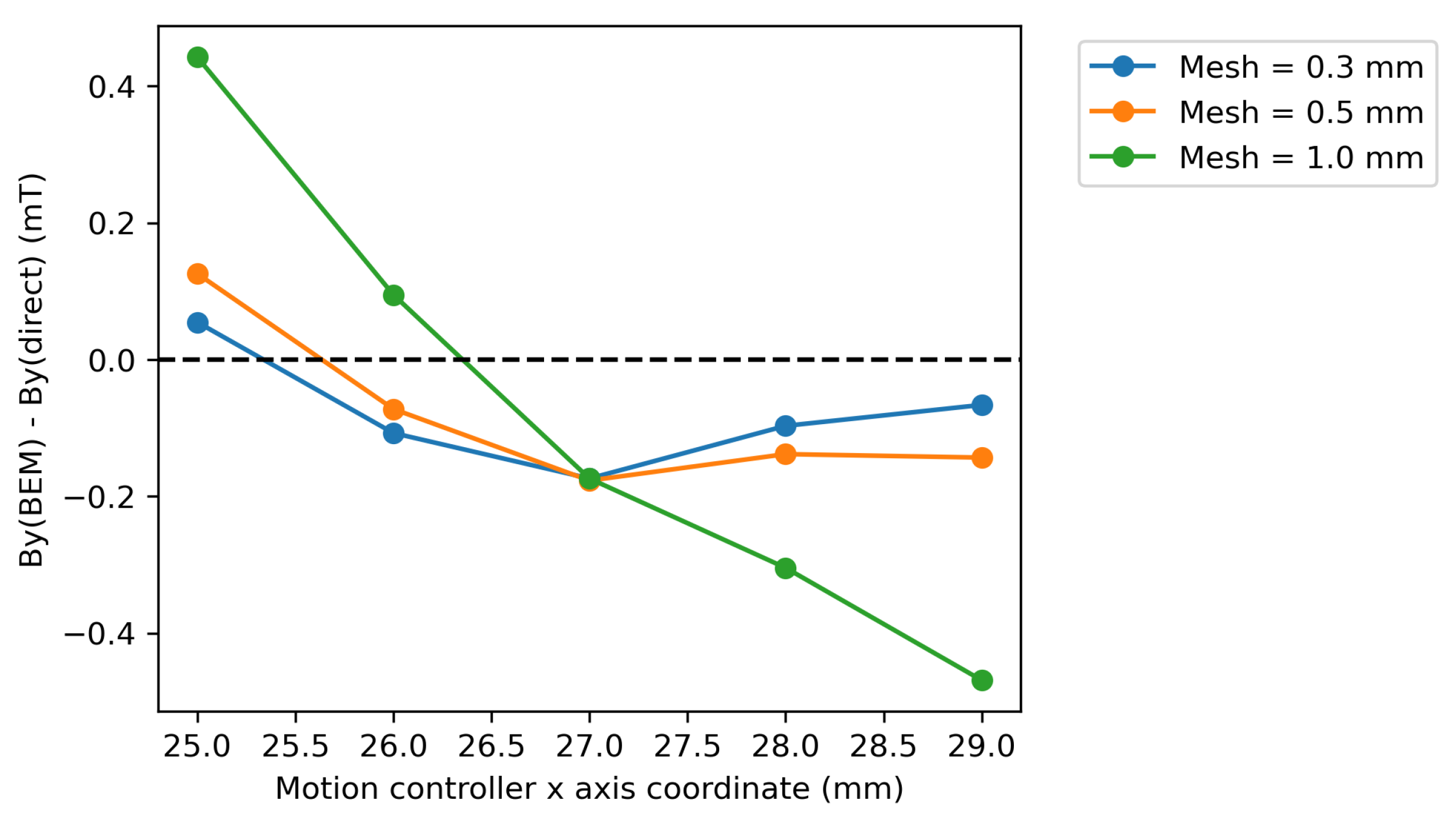
Figure 5 shows a plot of the difference between the $B_y$ field components measured directly to those constructed using different BEM mesh sizes over the same axis, as shown in Figure 4, but with a reduced range to be within one measurement point of the boundary. From this plot, using a smaller mesh size results in the reconstruction of fields which more closely resemble the directly measured fields along the given axis. This suggests that using a smaller mesh size results in more accurate reconstruction of the fields, at the expense of higher computational resource requirements and calculation times. 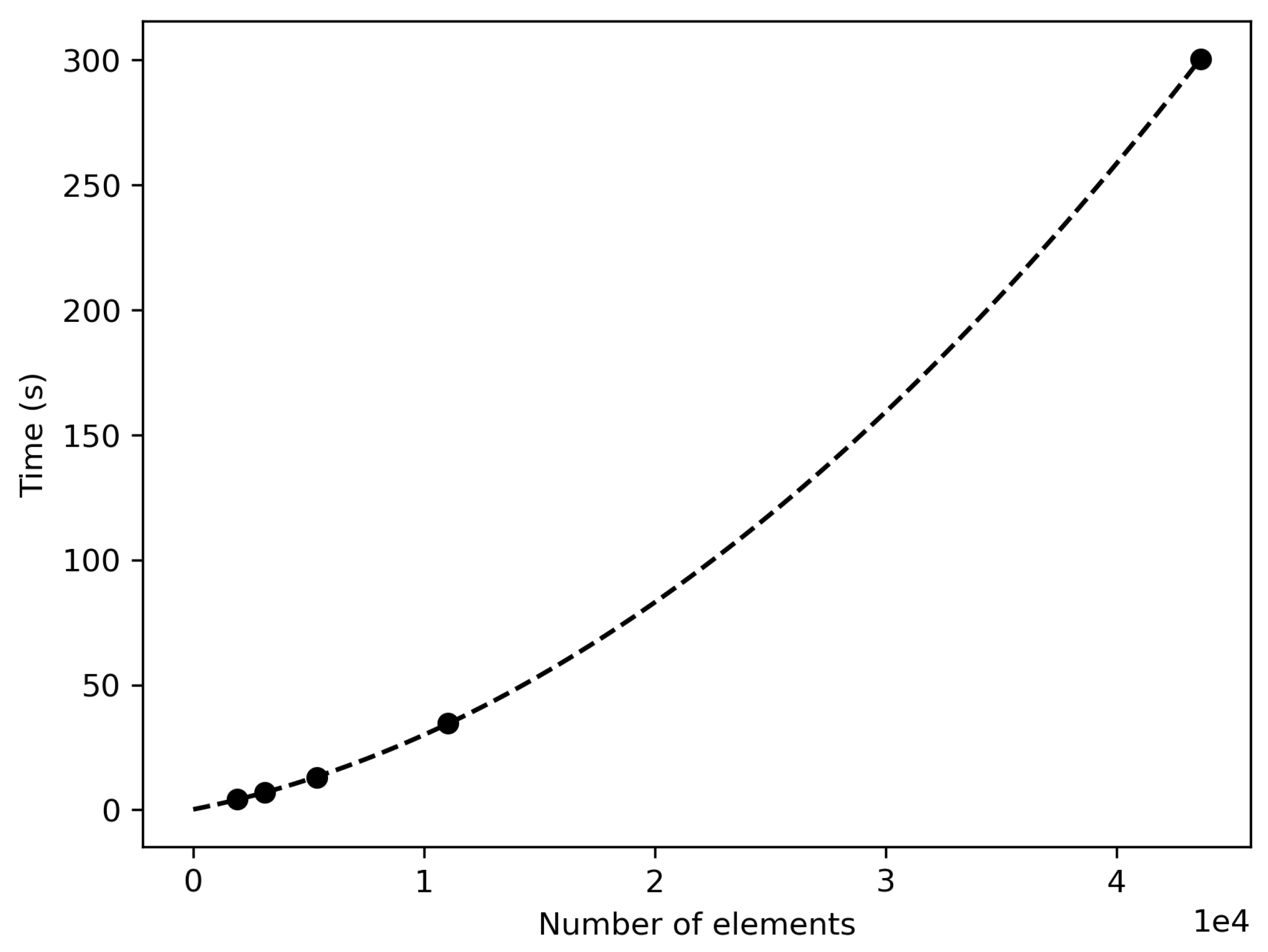The time required to solve the boundary integral equation (Equation (4)) scales with the square of the number of mesh elements, as shown in Figure 6.

Even at a 0.3 mm mesh size, the differences between the BEM-reconstructed and directly measured fields are larger than the uncertainty on the magnitude of the directly measured point fields. The uncertainty on the directly measured $B_y$ field component, from averaging the Hall sensor signal over 1000 samples, is 0.006 mT. The plots in Figure 5 suggest that further decreasing the mesh size would result in improved agreement with the directly measured fields. However, for a more dense mesh, more dense matrix calculations must be performed, and 0.3 mm was found to be a lower practical limit with the PC used to perform the calculations.

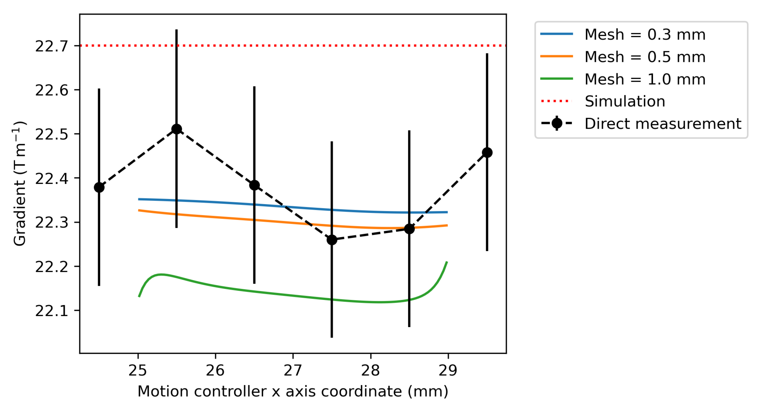
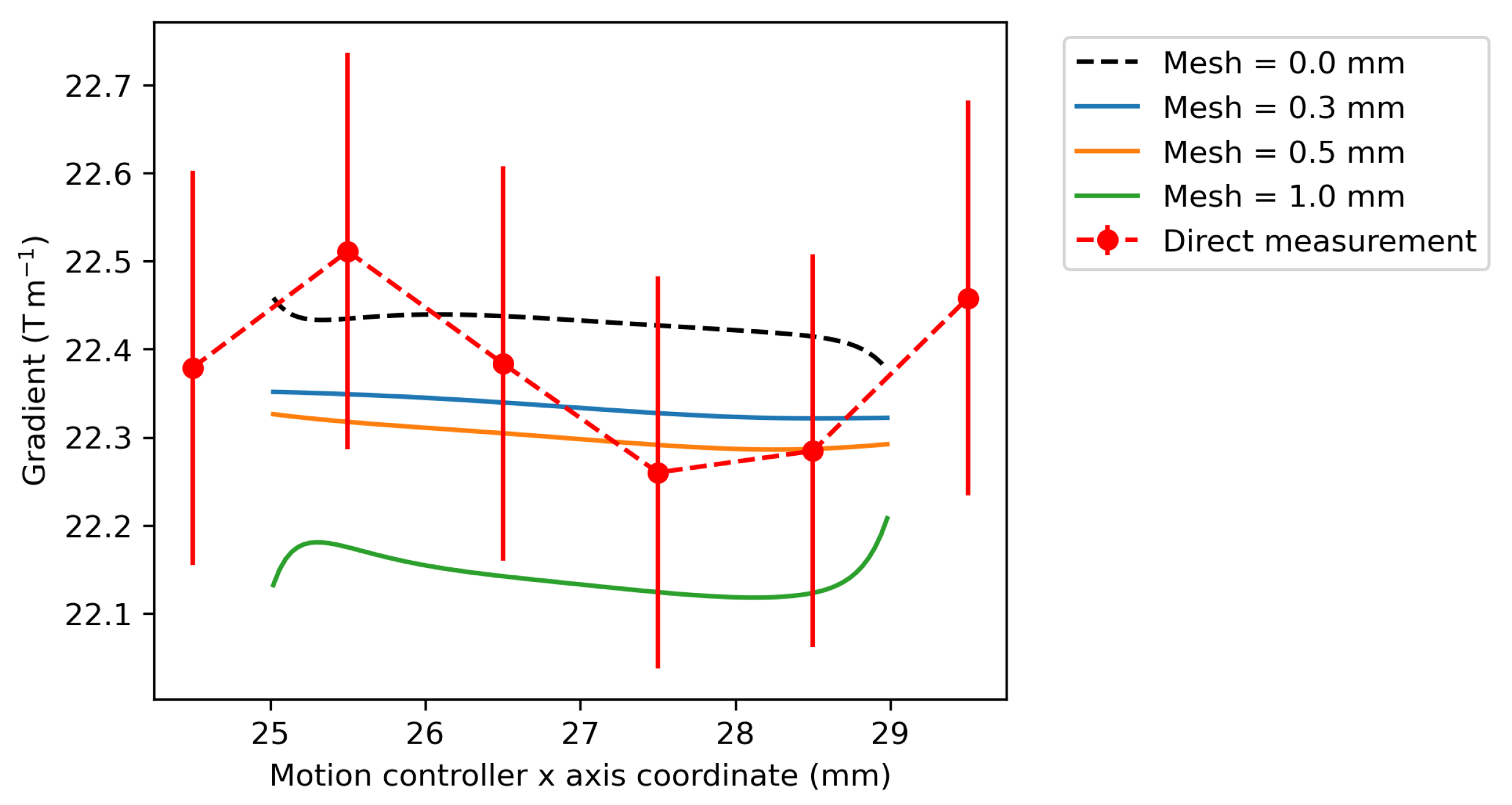
For a quadrupole magnet, the quantity of most relevance for particle tracking is the field gradient. Figure 7 shows the gradient of the $B_y$ field component along the same x-axis calculated by numerical differentiation of the directly measured points and the BEM fields reconstructed for different mesh sizes. The error bars on the directly measured points are dominated by the uncertainty in the position of the Hall probe, defined by the precision of approximately ±5 μm on the motor controller x stage and measured by absolute encoders. Each field point is an average of 1000 samples collected at that point, with an average standard deviation per point of 0.006 mT. For a mesh size of 1.0 mm, the reconstructed gradient is lower than the gradient calculated from the directly measured field points. As the mesh size is reduced, the magnitude of the reconstructed gradient more closely approaches the directly measured gradient. For mesh sizes of 0.3 and 0.5 mm, the BEM gradient is within the error bars of the directly measured gradient values. This shows good agreement with the direct measurements. The red dotted line represents the field gradient predicted from the Opera simulation off 22.7 T m⁻¹ [27]. The simulated gradient is greater than the directly measured and BEM gradients. This is mostly likely explained by differences between the BH curves of the used magnet blocks and the idealised curves used in the simulations [28].

A point of note is that the field gradient profiles calculated using the BEM vary much more smoothly than those by direct measurement. This is because, for the directly measured values, uncertainties on the exact locations of adjacent measurements stack to lead to a larger uncertainty on the gradient values calculated by numerical differentiation. For the BEM fields, the output of the BEM model is the scalar potential, which is a solution to Laplace’s equation (Equation (2)). The magnetic fields are calculated by differentiation of this potential using Equation (1). This means that the solution for the BEM fields is forced to have zero divergence. Therefore, these fields conform to the Maxwell equations and form a valid magneto-static solution. Consequently, the BEM fields demonstrate a realistic physical behaviour, which could describe a real magnetic field. The same cannot be said for the directly measured fields. Furthermore, by integrating over the boundary, random errors in the Hall sensor reading and motor controller position are cancelled [20], improving the accuracy of the gradient calculations compared to the numerical differentiation of the direct measurements.

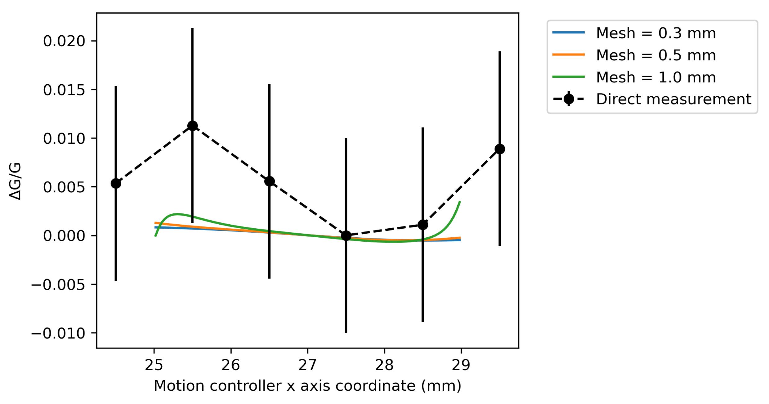
BEM is likely a more useful tool for estimating the gradient homogeneity than by using a direct measurement along a single axis scan. A typical specification on the gradient homogeneity ($\Delta$G/G) for a quadrupole magnet is 1 × 10⁻³. For a step size of 1 mm ± 5 μm, the uncertainty in the gradient homogeneity from the positional uncertainty is 5 × 10⁻³, which already exceeds the target specification. The homogeneity, relative to the centre of the scan, is shown in Figure 8 for the directly measured and BEM values at different mesh sizes. The directly measured gradients show much worse homogeneity values than those calculated using the BEM due to the uncertainties in the stage positions. The BEM gradients all show much more conservative predictions of the homogeneity within one mesh size of the boundary. In particular, the 0.3 mm, 0.5 mm and 1.0 mm mesh sizes show good agreement in the range between 26 mm and 28 mm. The BEM has the effect of smoothing out the uncertainties across all of the point measurements and ensures that the computed fields have the correct physical properties. Therefore, using the BEM is a more accurate approximation to the homogeneity of the field gradient.

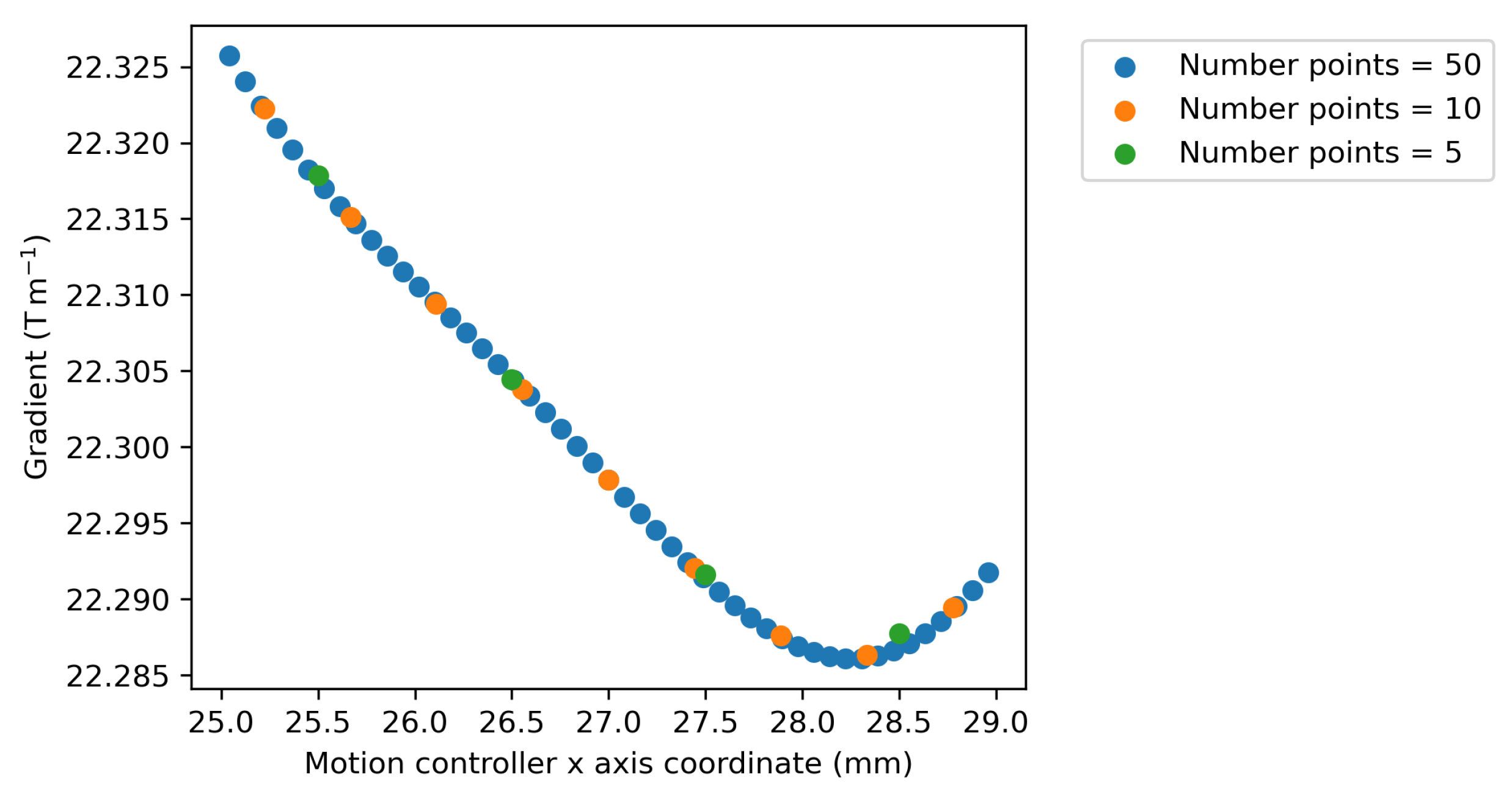
The uncertainty in the gradient calculated by the numerical differentiation of direct measurements can be reduced by using larger step sizes between points, at the expense of the resolution of the measurement. By comparison, the fields can be evaluated with arbitrary resolution using the BEM without any loss in accuracy. This is shown in Figure 9, where the gradient is evaluated by the numerical differentiation of the BEM field calculated using a 0.5 mm mesh where a different number of points are plotted along the x-axis. As the number of points is increased, the resolution of the gradient shape is increased. There is a good overlap between the plots for differing numbers of points used for the differentiation, showing that a large number of points can be used to improve resolution without a loss in accuracy.

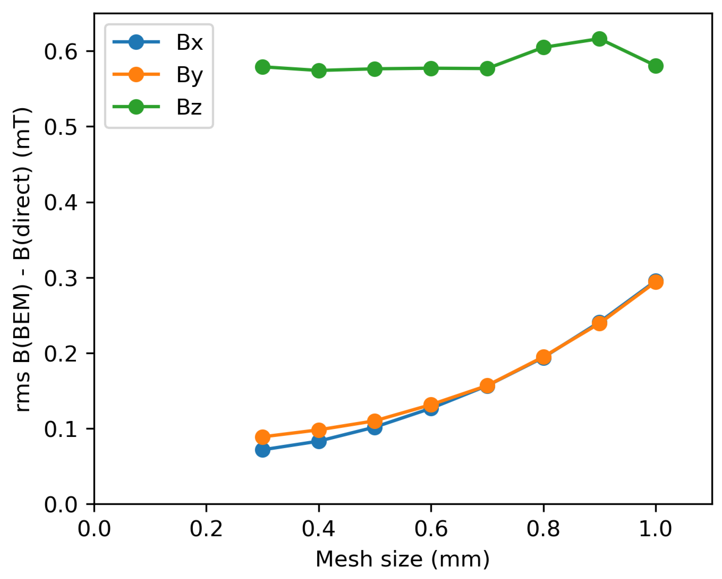
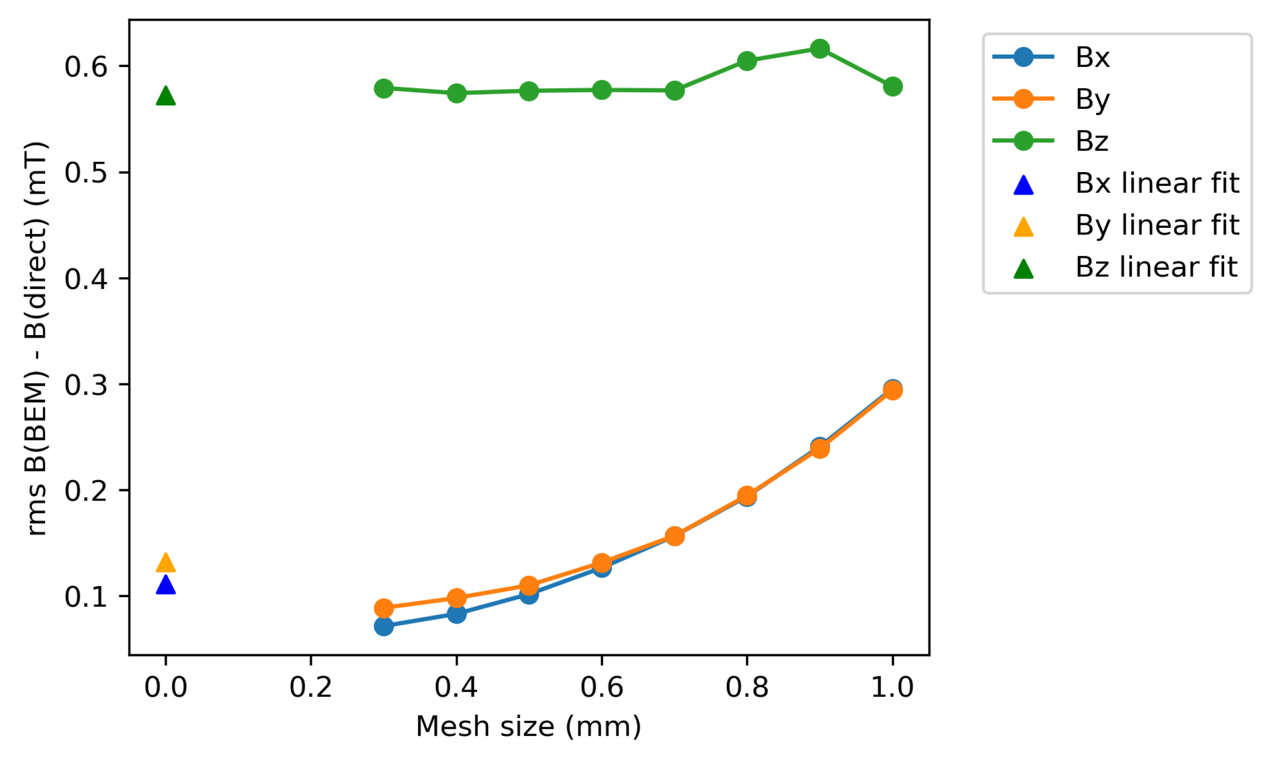
To test the accuracy of the BEM field reconstruction, the magnitudes of the field components were compared for the direct measurement and BEM reconstruction for each of the discrete points within the measurement grid. For each point, the difference between the directly measured and BEM field components were calculated. The root mean square (rms) difference between directly measured and BEM fields was calculated for each field component as a function of the BEM mesh size. For each mesh size, only points greater than one mesh length from the boundary were included in the analysis to avoid overestimating the rms errors. The results are shown in Figure 10. It is apparent that, as the mesh size is decreased, the rms difference between the BEM and directly measured transverse and vertical components of the magnetic field is decreased. As the mesh size decreases, there are more evaluations of the field components normal to the boundary, and so finer details in the shape of the field can be captured, leading to a closer reconstruction of the directly measured fields. It is not expected that the reconstructed fields will ever exactly fit the measured data due to the random errors introduced by measurement noise. The directly measured points on the grid are subject to several sources of uncertainty: the uncertainty in the averaged field magnitudes, the positioning of the motor stages and the systematic roll, tilt and yaw angles of the probe with respect to the motion control axes. The BEM reconstruction acts to smooth out the random uncertainties and gives a viable magneto-static solution for the magnetic field.

The green line in Figure 10 shows the rms difference between the BEM and directly measured axial component of the field ($B_z$). In this case, there appears to be little benefit to decreasing the mesh size. The axial field measured is very low. In the case where the magnet, motion control bench and Hall sensor are perfectly aligned, no axial field should be measured at any point other than at the fringe fields of the magnet. The difference between the directly measured and BEM axial fields may be due to a systematic misalignment between the Hall sensor and the motion controller coordinate system. The axial field is of less concern than the transverse field components for determining the effect of the field on a particle beam. Therefore, a reduced accuracy in the axial field component will not impact the accuracy of determining the focussing properties of the quadrupole. The rms difference between the BEM and directly measured axial field components is below 0.6 mT.

The blue and orange lines in Figure 10 are for the $B_x$ and $B_y$ transverse and vertical field components. The shape of these lines suggest that a further reduction in the mesh size would result in a closer agreement between the directly measured and BEM fields. The disadvantage of further reducing the mesh size is in the increased density of the required matrix calculations and hence increase in required computing resources. For the PC used to perform these calculations, a 0.3 mm mesh size was the minimum that could be solved before errors related to insufficient memory were encountered.

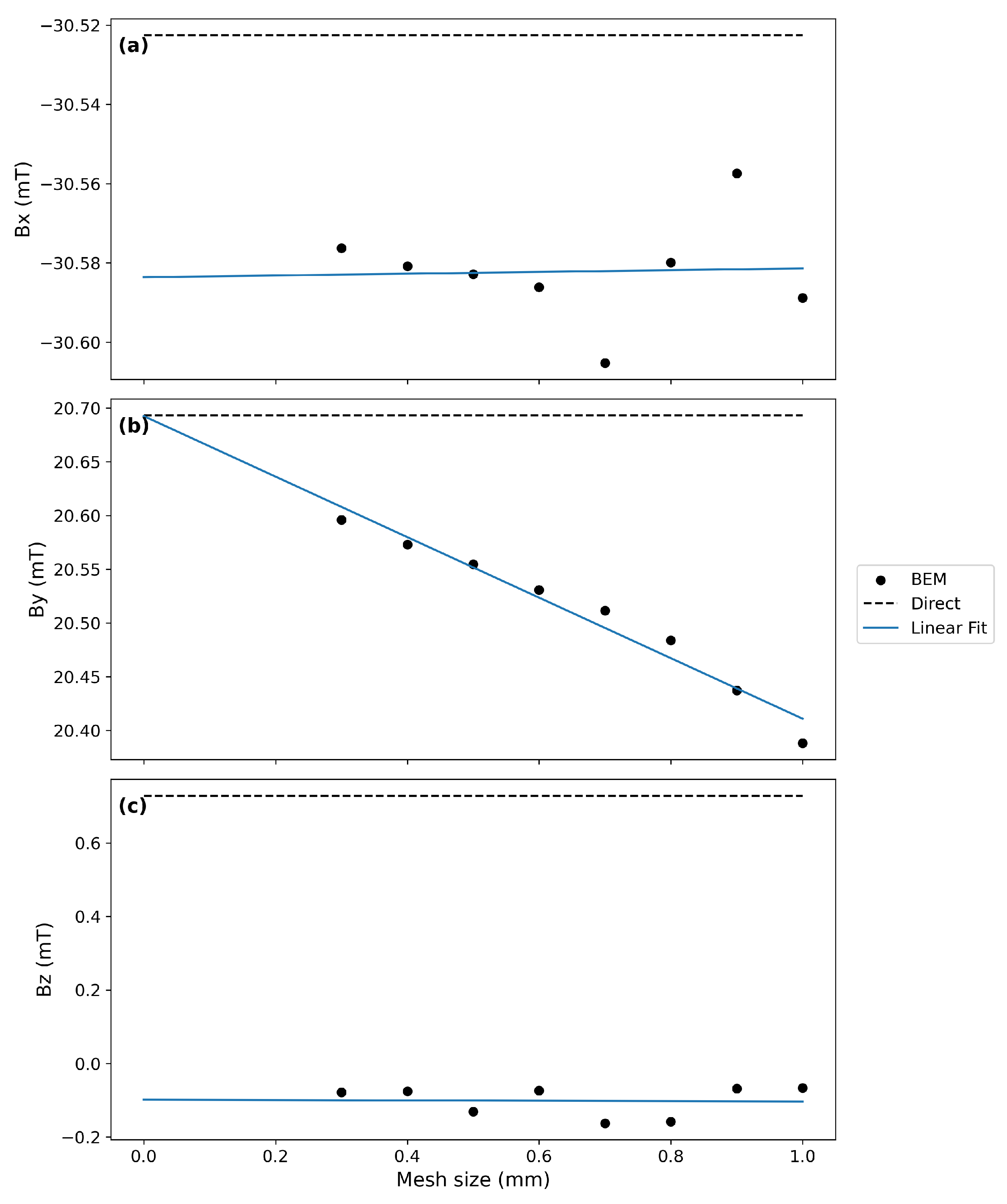
If the field components at a given coordinate are evaluated using the BEM at multiple mesh sizes, it is possible to extrapolate the predicted field reconstructions to infinitesimally small mesh sizes. Figure 11 shows an example of extrapolation to a “0 mm” mesh size for the field components evaluated at a single point near the centre of the measurement volume (x = 28 mm, y = 8 mm, z = 65 mm). For each plot, the black points show the BEM-calculated field component at that mesh size, the black dashed line shows the value of the directly measured field component and the blue line show a linear fit to the BEM data.

Figure 11a shows the $B_x$ field component. There appears to be no evident trend in the magnitude of the BEM-calculated $B_x$ field with reducing mesh size, as shown by the linear fit. Extrapolating this fit to 0 mm mesh size does not provide a significantly better agreement with the directly measured value than for the BEM field at 0.3 mm mesh size. The difference between the extrapolated and directly measured field component is approximately 0.06 mT.

The results for the $B_y$ field component are shown in Figure 11b. Here, there is a much clearer trend between mesh size and field strength. The linear fit predicts a significantly better agreement with the directly measured field at the extrapolated 0 mm mesh than for the 0.3 mm mesh size.

Finally, the results for the $B_z$ field component are shown in Figure 11c. There is little trend between the magnitude of the BEM field component with mesh size and the linear fit shows little improvement in the agreement with the direct measurement.

These results show that a reducing mesh size tends to result in a closer agreement between the BEM and directly measured field components, at least for the $B_y$ field component. A linear fit may be used to extrapolate what the BEM field is expected to be at an infinitesimally small mesh size, which is predicted to give a more accurate field component evaluation than for a single evaluation at one mesh size.

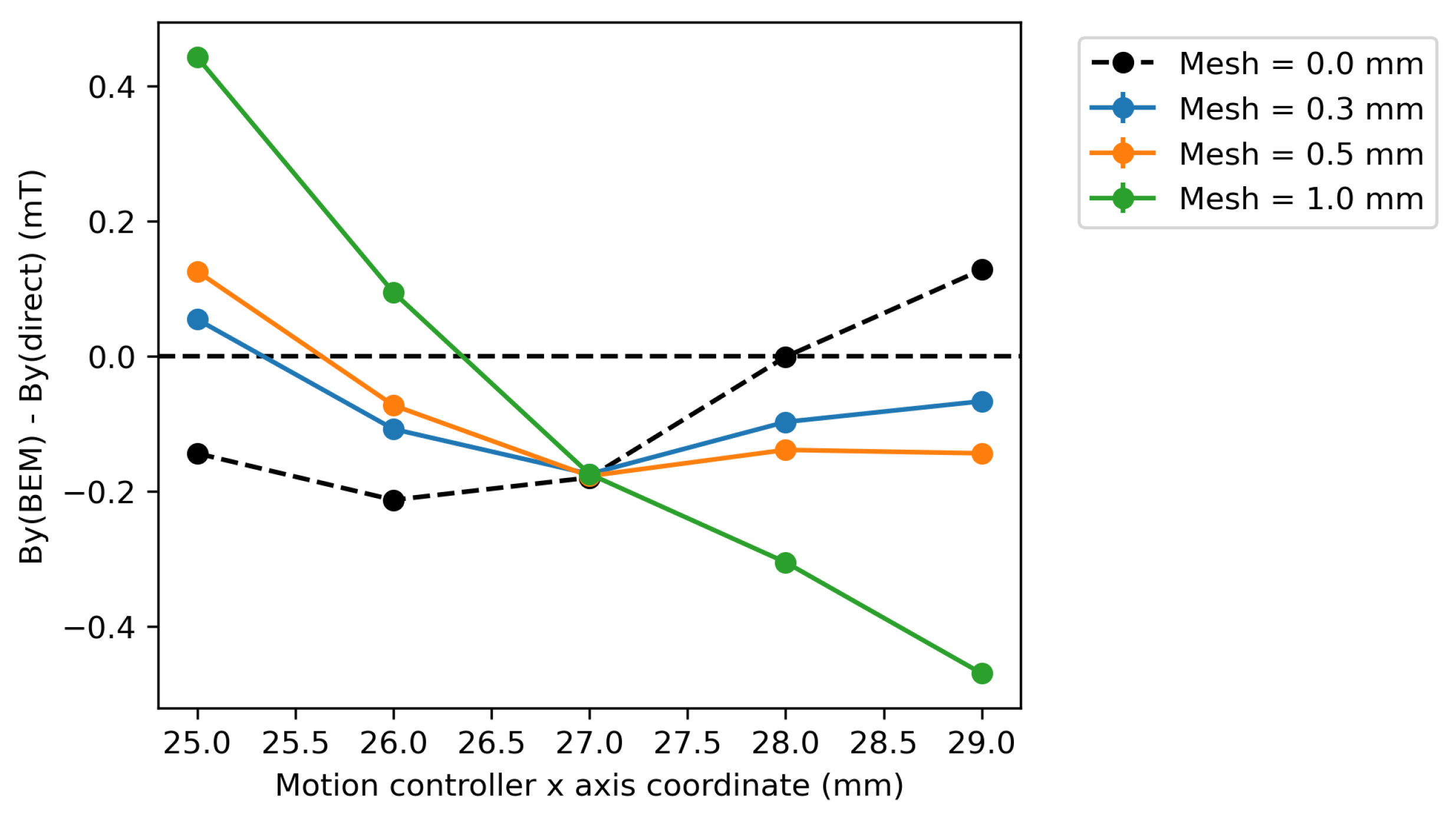
Figure 12 shows a plot of the $B_y$ field component along the motor controller x-axis at the point y = 8 mm, z = 65 mm. The black dashed line shows the $B_y$ field component calculated by the extrapolation of a linear fit from the BEM fields calculated at mesh values between 0.3 and 1.0 mm in steps of 0.1 mm. It is apparent that the use of the linear fit does not universally result in a better agreement with the direct measurement, as was predicted from Figure 11. In the centre of the plot, the fields at different mesh sizes do not vary greatly, resulting in no greater agreement being achieved by the extrapolation. At the point x = 28.0 mm, the extrapolation gives a good agreement with the directly measured field. Towards the edges of the plot, the extrapolation overshoots, resulting in a poorer agreement with the direct measurement than for the 0.3 mm mesh size. This gives an indication that a linear extrapolation of the fields at a given point will not necessarily result in a more accurate agreement with directly measured fields.

The gradients of the lines plotted in Figure 12 are shown in Figure 13. Here, it can be seen that the gradient calculated from the extrapolated fields at 0 mm mesh size are within the error bars of the gradient calculated by numerical differentiation of the directly measured field points. The shape of the gradient is clearly influenced by the changing gradient with reducing mesh size. Therefore, this shape is highly dependent on the fields evaluated at different mesh sizes. Computing the shape of the gradient using the extrapolated fields is unlikely to be an accurate way of determining the gradient homogeneity as the extrapolation does not maintain the magneto-static solution to the fields imposed by the BEM.

To determine the overall accuracy of the extrapolation method, the field components were evaluated at multiple mesh sizes and extrapolated to 0 mm mesh size for each of the discrete points on the measurement grid. The rms difference between the extrapolated field components and the directly measured components were then calculated. This was performed for discrete points within one measurement step within the boundary and for a linear fit to the field components at mesh sizes from 0.3 to 1.0 mm in 0.1 mm steps. The results are shown in Figure 14. It is apparent that extrapolating the value of the field component at each discrete point to 0 mm mesh size does not result in the low rms difference between the BEM and directly measured fields that was predicted using Figure 10. Instead, the extrapolation method results in larger rms differences than for the fields computed using the 0.3 mm BEM mesh. This suggests that there is no increased accuracy that can be achieved by using the extrapolation method.

In many cases, the relative field error is of more interest than the absolute field error. For these measurements, the relative field errors can be difficult to quantify because, at certain points, the absolute values of the measured fields are low. Therefore, small absolute differences result in large relative differences. This is demonstrated in Figure 15, which plots the absolute relative difference between the directly measured and BEM fields as a function of the magnitude of the directly measured field component at a point for the 0.3 mm mesh size. It is apparent that, for larger absolute fields, the relative error between the BEM and directly measured fields reduces for all three field components. 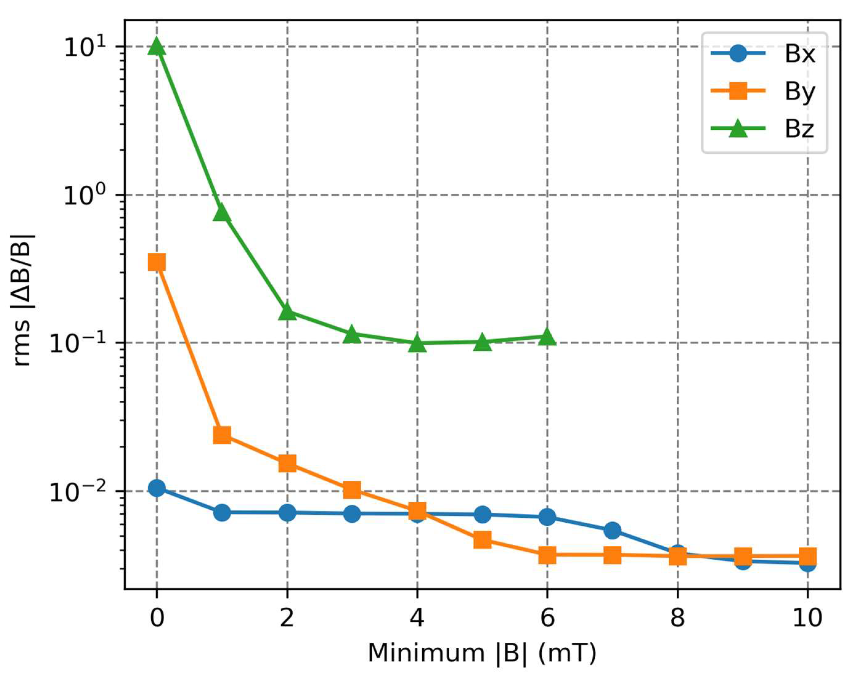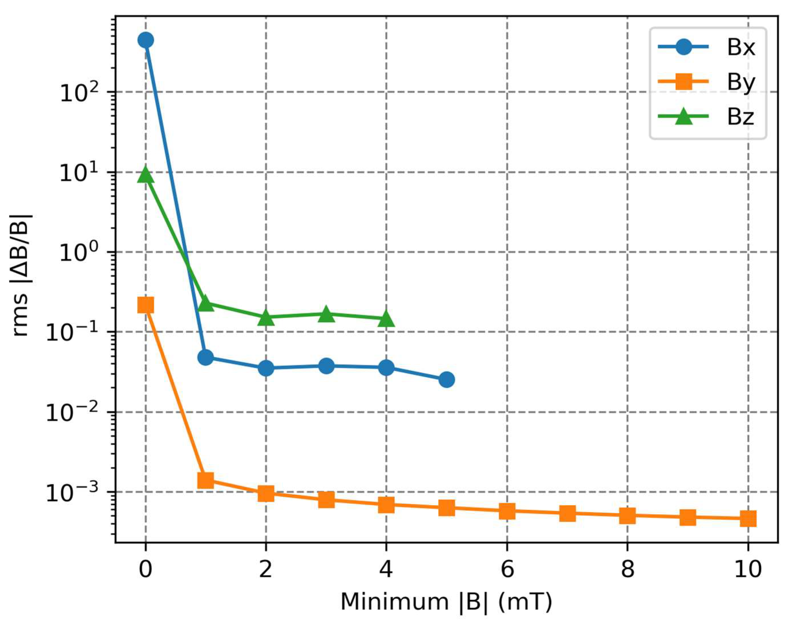This is further demonstrated by Figure 16, which plots the rms relative field error between the BEM and directly measured fields, where only the directly measured field components above a set magnitude are used for the calculation. For all three field components, the rms relative field error decreases as the minimum considered field magnitude is increased. For the $B_x$ field component, this affect is only slight and not easily visible on the plot.The rms relative field error decreases rapidly with increased minimum field before converging to a point. For field components greater than 1 mT, the rms relative differences between the directly measured and BEM fields are 0.7%, 2.4% and 76.5% for the $B_x$, $B_y$ and $B_z$ field components, respectively. The large rms relative difference for the $B_z$ field component is due to the low average magnitude of the directly measured field components.

Overall, the BEM has been used to reconstruct the fields inside the 3D measurement grid of the ZEPTO-Q3 quadrupole. As the mesh size used for the BEM calculations is reduced, a better agreement is achieved with the directly measured fields, at the expense of computing resources. For a mesh size of 0.3 mm, the rms absolute differences between the directly measured and BEM fields are 0.072 mT, 0.089 mT and 0.579 mT for the $B_x$, $B_y$ and $B_z$ field components, respectively. These are two orders of magnitude greater than the standard deviations on the directly measured fields of 0.006 mT. The rms relative field errors for the three field components are 3.7%, 2.7% and 82.2%, respectively.

4. ECRIS Dipole

The second magnet that has been tested was a tuneable permanent magnet dipole designed and built for use on an Electron Cyclotron Resonance Ion Source (ECRIS) beamline for $M/Q$ separation of ion species [32]. The magnet was designed to have a tuneable strength to allow charge state selection in prototyping experiments to develop a net zero ion beam analysis facility. This dipole was built and measured at Daresbury Laboratory. Like the ZEPTO-Q3 quadrupole, one of the tests involved a scan over a 3D volume, measuring the field components at each discrete point on the scan using the Senis Type C 3-axis Hall sensor and 3MH6 Teslameter. The measurement was over a volume measuring 80 × 20 × 300 mm³ with a 2 mm step size along each of the x, y and z axes. This resulted in a grid containing 68,101 points, which took 1.6 days to measure. Conversely, the boundary consists of only 15,802 points and so would have taken only 0.4 days to measure, approximately a quarter of the total measurement time. This highlights the time-saving advantages of using the BEM to measure large volumes. An image of the engineering model of the dipole is shown in Figure 17. The zoomed-in image shows a red cuboid indicating the measurement volume. The grey grid represents the discretisation of points on the surface of the volume. 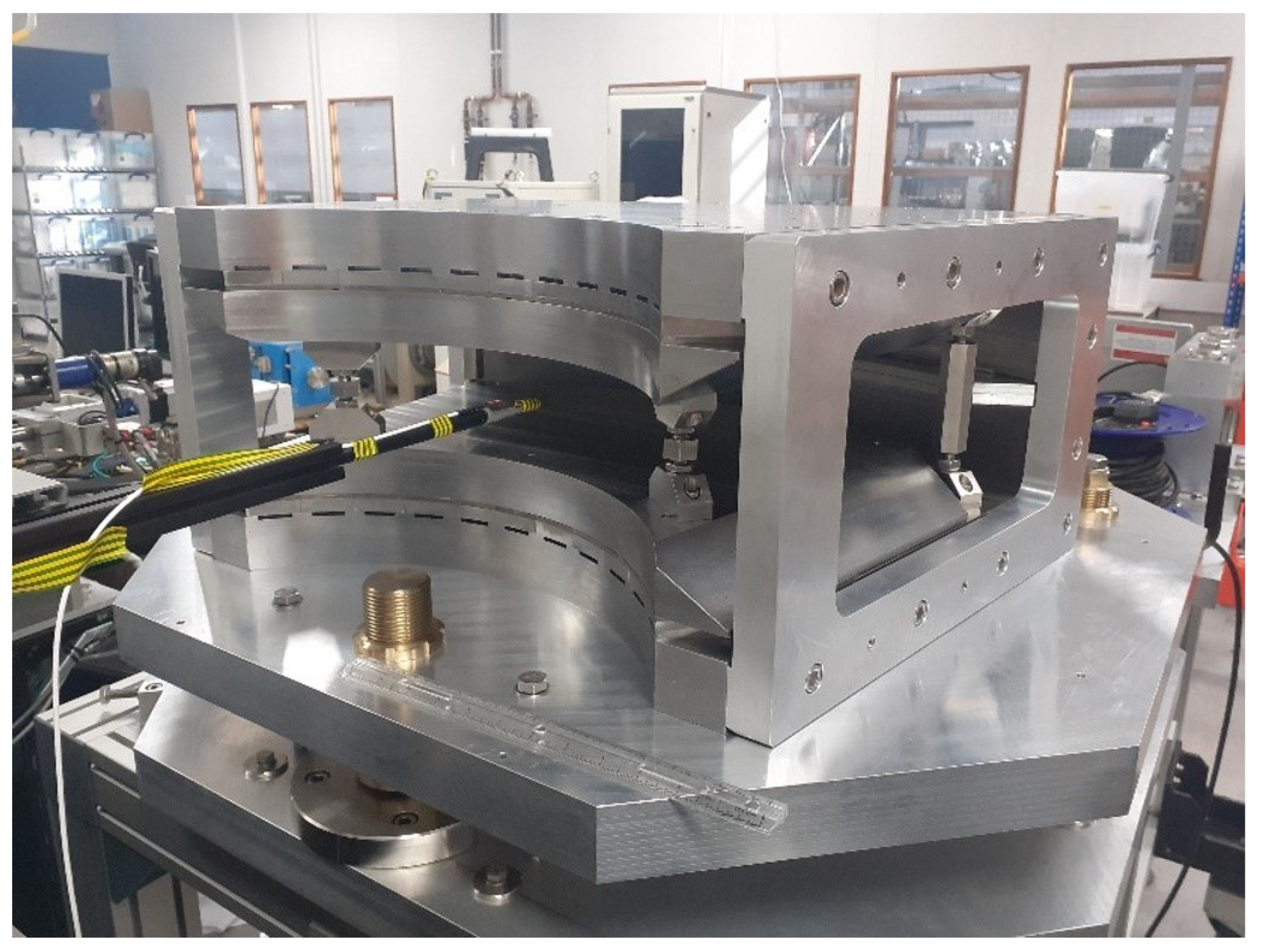Figure 18 shows a photograph of the magnet being measured on the bench. In this orientation, the probe holder arm is parallel to the motion coordinate x-axis. For the grid measured, the probe holder was rotated by 90 degrees so that it was parallel to the z-axis to allow for measurements from the centre of the magnet to a point outside the magnet, without clashing with the mechanical supports.

Figure 19 shows contour plots of the magnetic field magnitude and direction in the transverse (xy) plane of the dipole magnet at a z coordinate inside the dipole (z = 2900 mm). Figure 19a shows the contours for the points directly measured with the Hall sensor, whilst Figure 19b shows the field contours reconstructed using the BEM with a 2 mm mesh. The plots show the same direction and general magnitude, indicating that the BEM provides an accurate reconstruction of the fields. The most obvious difference between the plots is that the direct measurements show more measurement noise, characterised by the lighter and darker regions, which are dispersed over the plane. The BEM fields vary more smoothly than the direct measurements. The relative differences between the magnetic field magnitude are shown in Figure 19c. The differences are in the range −0.4 to +0.4 %, with the largest differences being in the areas of measurement noise observed in Figure 19a.

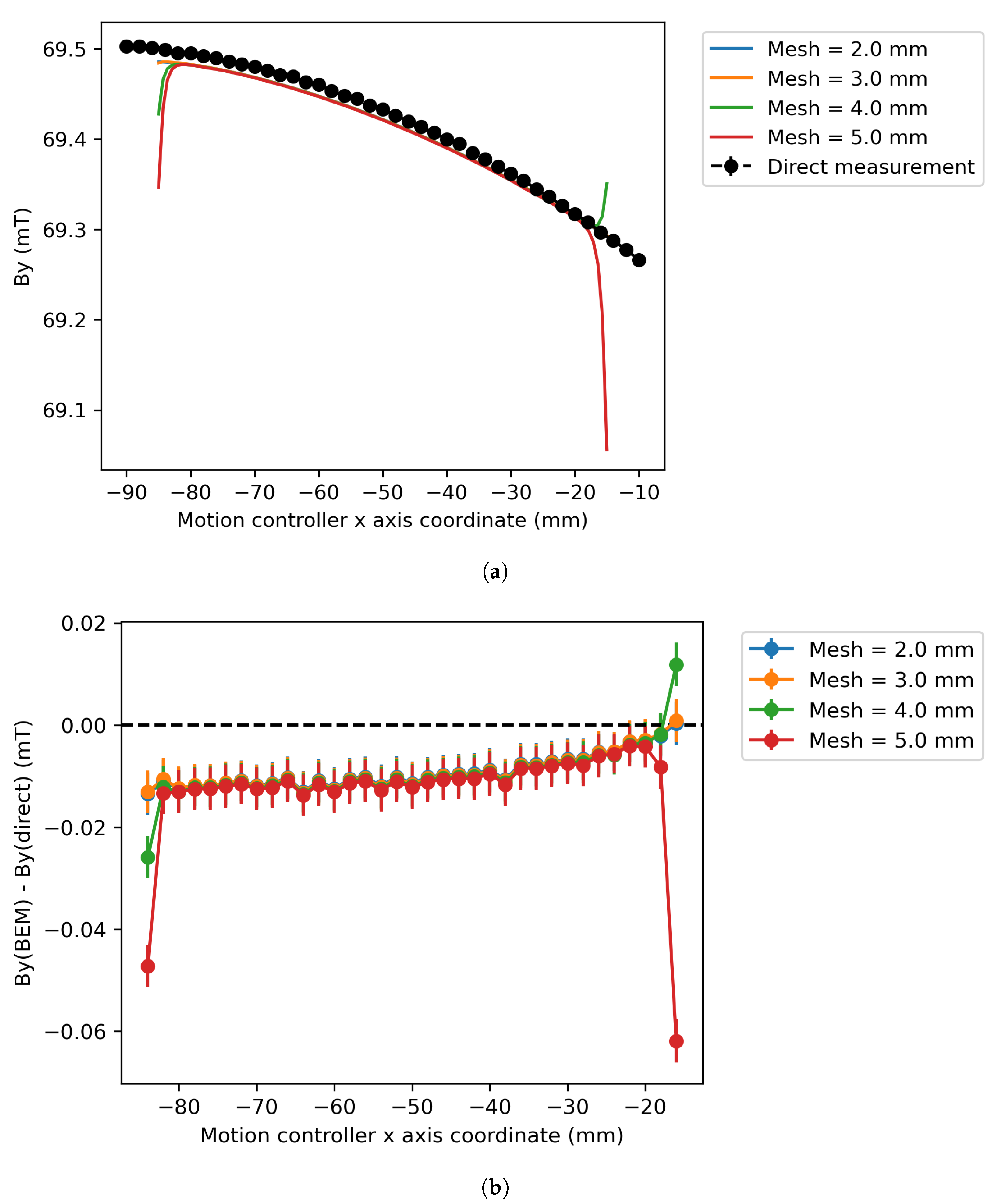
Figure 20 shows an example plot of the $B_y$ field component measured along the transverse (x)-axis at a plane inside the dipole magnet. Plot Figure 20a shows the field components alongside the directly measured fields. This plot shows a good agreement between the BEM fields and the directly measured fields in the centre of the measurement axis. Towards the ends, the agreement quickly becomes worse. This point happens closer to the centre of the measurement for larger mesh sizes. Figure 20b shows the differences between the BEM and directly measured fields. Apart from towards the end of the travel, where the BEM diverges, the differences between the BEM and direct measurements are all within 0.02 mT. The differences are all greater than the uncertainties on the direct measurements. This suggests that the BEM underestimates the true magnitude of the dipole field. There is significant overlap of the plots for the different mesh sizes in the centre of the plot. Therefore, there is little gain to be had from further reducing the mesh or extrapolating the fields to 0 mm mesh size.

Figure 21a shows a plot of the $B_y$ field components measured along the motion controller z-axis from a point outside of the dipole (where the field tends to 0) to a point inside the magnet, where the field is approximately 70 mT. The plot shows a very close agreement between the directly measured fields and those reconstructed using the BEM. Figure 21b shows the difference between the directly measured and BEM fields. As with Figure 20, there is little difference between the different mesh sizes, and the BEM appears to consistently underestimate the magnitude of the field inside the dipole. In the low field region up to approximately z = 2750 mm, the uncertainties on the differences overlap with the directly measured value. The differences between the directly measured fields and the BEM peak at approximately z = 2850 mm. This is the point within the fringe field of the dipole, where the field is changing most rapidly. Based on the plots, reducing the mesh size does not significantly improve the agreement between directly measured and BEM fields in this region. Future measurements may benefit from taking a finer set of direct point measurements in regions of rapidly changing field strength to allow a more accurate interpolation of the field in these regions.

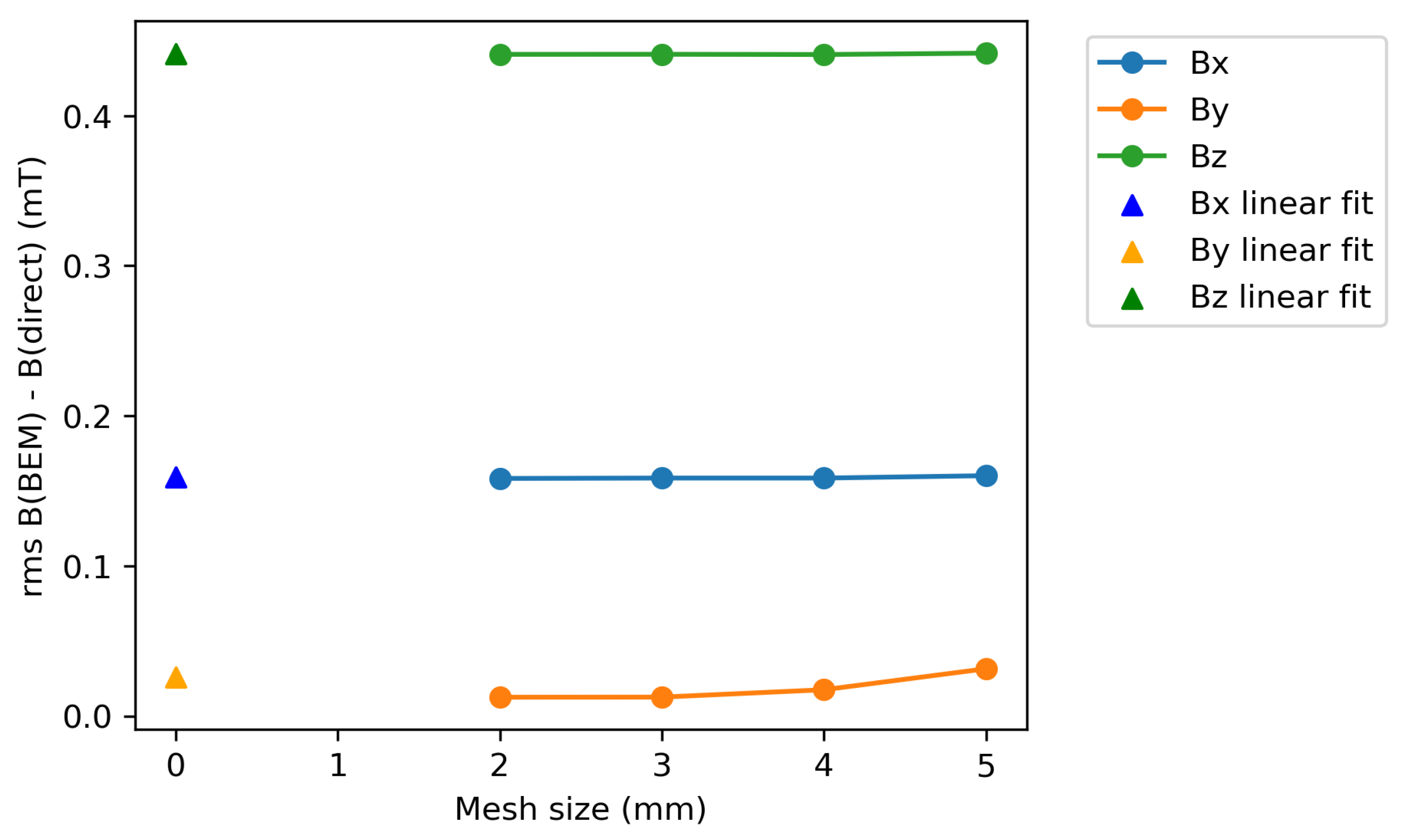
To assess the overall accuracy of the BEM calculations with respect to the direct measurements, the rms difference between the directly measured field components and BEM field components at all of the discrete points in the measurement grid within 5 mm of the boundary were calculated as a function of mesh size. The results are shown in Figure 22. The rms difference between the directly measured and BEM-calculated $B_x$, $B_y$ and $B_z$ components all show little change with changing mesh size. At a mesh size of 2 mm, the rms differences between directly measured and BEM fields are 0.16, 0.01 and 0.44 mT for the $B_x$, $B_y$ and $B_z$ field components, respectively. These are all greater than the average uncertainties on the point measurements of 0.008, 0.004 and 0.005 mT for the $B_x$, $B_y$ and $B_z$ fields, respectively. Therefore, the differences between BEM and direct measurements are larger than the uncertainties on the direct measurements. The directly measured $B_y$ field components in the centre flat region of the magnet were within 0.5 mT of the expected values using nominal magnetisation strengths in the magnetic design simulations using Radia3D [32]. This difference from the simulations is greater than the rms difference between the measured and BEM component of 0.01 mT. Therefore, the BEM reconstruction provides no loss in accuracy compared to the direct measurements with respect to the simulation.

Included in Figure 22 are the rms differences between direct and BEM fields where fields at each point are extrapolated to 0 mm mesh size using a linear fit, which are shown by triangles. For the $B_x$ and $B_z$ field components, extrapolating to 0 mm mesh size makes little difference to the rms differences. This is because changes to the mesh size do not significantly change the BEM-calculated field components. In the case of the $B_y$ component, the extrapolation leads to a larger rms difference than for the case using a 2 mm BEM mesh. As with the ZEPTO-Q3 results, the extrapolation leads to a poorer agreement and results which do not necessarily form a solution to the Laplace equation.

The mesh reduction seems to have little impact on the rms differences between directly measured and BEM fields for the ECRIS dipole, unlike for the ZEPTO quadrupole. This may be because the field changes less rapidly for the dipole than for the quadrupole. Therefore, a higher resolution in the mesh is not required to better capture the changes in the field. Therefore, for future work, it may be necessary to ensure that a fine grid of measurements is used to measure multipole fields with large field gradients. Another difference between the ZEPTO-Q3 and ECRIS dipole measurements is that the ECRIS measurements were made on a regular grid, with the same step size (2 mm) between points along all three axes, whereas for the ZEPTO measurements, the step size along the z-axis (5 mm) was larger than along the transverse (x) and vertical (y) axes. Future measurements should focus on taking measurements over grids with equal spacing between the points along the coordinate axes to allow a mesh size comparable to the step size to be used and to avoid issues with over-meshing in regions where many mesh points are created between direct measurement points. To help improve the accuracy of the fields in regions of particular interest, it may help to take a more dense set of point measurements. The benefits of a variable measurement grid precision will be investigated in future work.

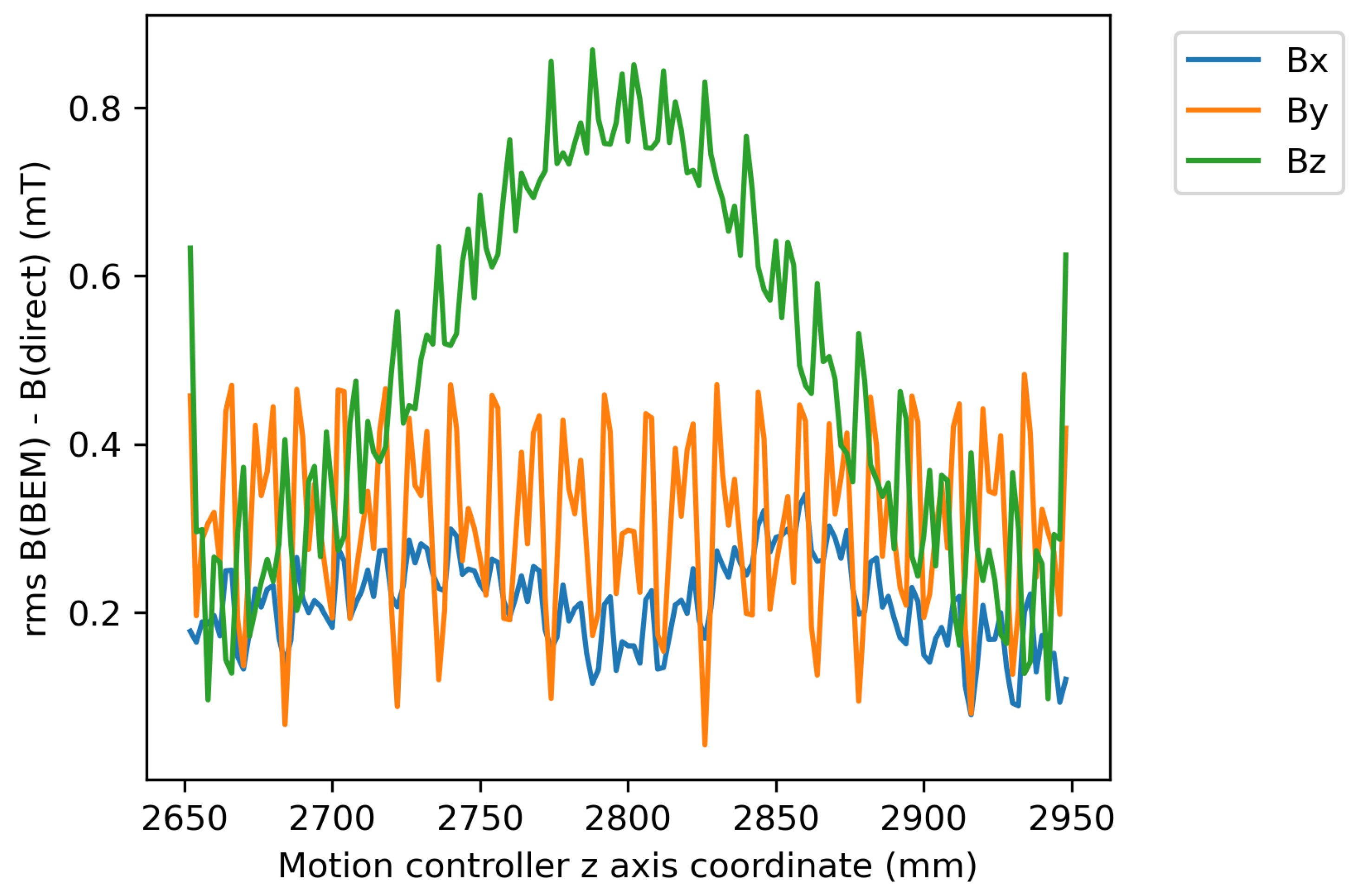
The fringe fields at the ends of the dipole magnet are of particular importance. The edge field and edge focusing is often critical for $M/Q$ separation magnets [33]. The fringe fields are not described by 2D multipole evaluation of the fields. Figure 23 shows a plot of the rms differences between directly measured and BEM field components as a function of the axial coordinate of the measurements. The plot shows no trend in the rms differences for the $B_x$ or $B_y$ field components with axial coordinate. This indicates that the absolute difference between the directly measured and reconstructed field components is independent of the local shape of the field. Therefore, the BEM can be used to just as accurately reconstruct the fringe fields as the fields in the bulk of the magnet.

It should be noted from Figure 23 that the difference between the $B_z$ components of the field does show a trend with axial position. The rms differences peak near the coordinate z = 2800 mm. This is near the centre of the fringe field where the field gradient is highest. The large differences are likely due to a lack of field data in the axial direction being captured by the BEM mesh. At the two planes of the boundary perpendicular to the z-axis (outside of and in the bulk of the dipole), the normal field tends to 0. It may be possible to gain a more accurate representation of the fringe fields by measuring a boundary around the region containing the fringe field only with a fine measurement grid. As the axial field is less important for measuring the bending and focussing effect of the fringe field on the beam, the larger rms differences between the directly measured and BEM fields for the axial than transverse components are not of concern for the use of the BEM in evaluating the fields.

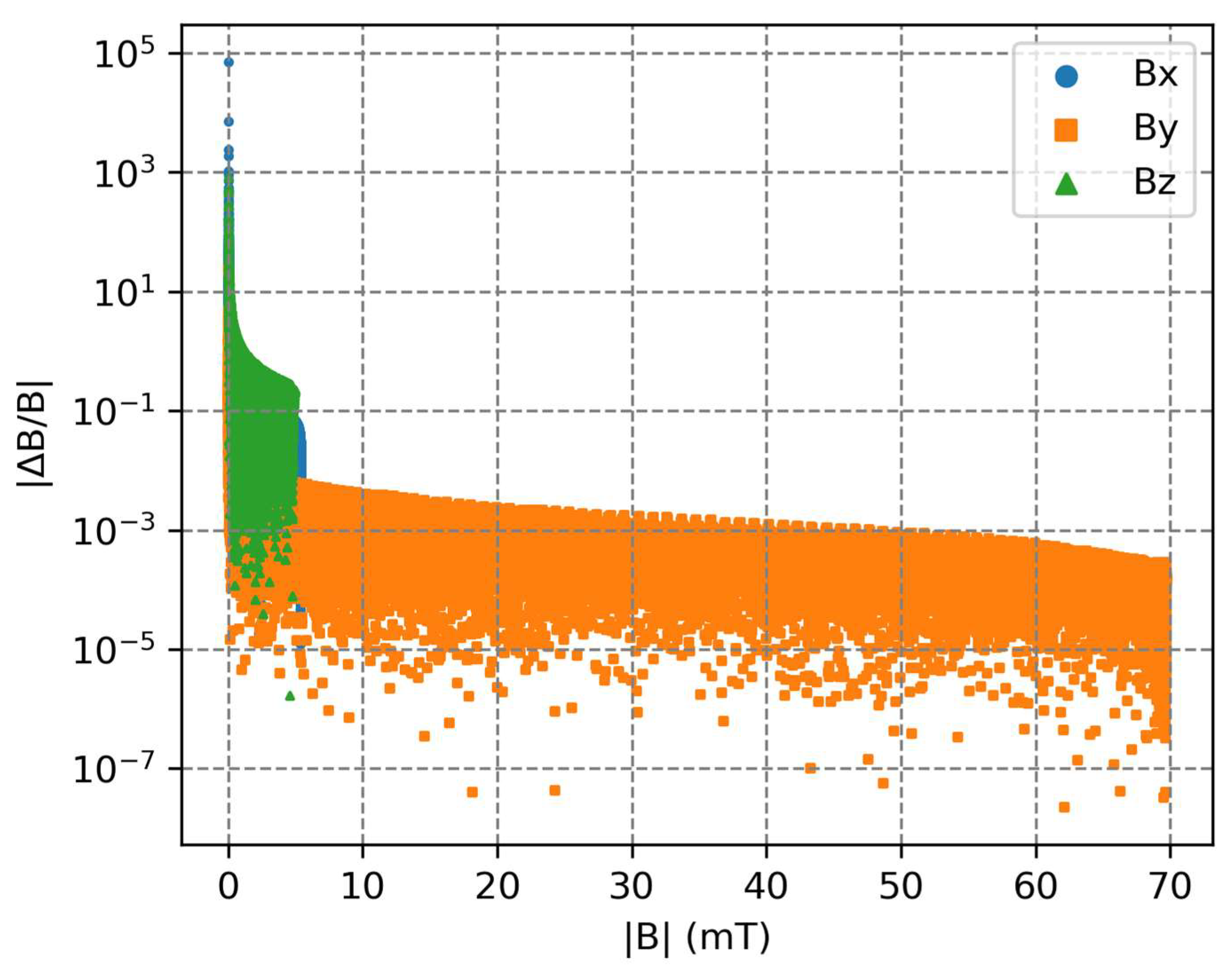
Figure 24 shows a plot of the absolute relative difference between the directly measured and BEM fields as a function of the magnitude of the directly measured field component at a point for the 2 mm mesh size. The relative error in the field components decreases for larger absolute measured field magnitudes. Figure 25 plots the rms relative field error between the BEM and directly measured fields, where only the directly measured field components above a set magnitude are used for the calculation. For all three field components, the rms relative field error decreases rapidly when fields greater than 1 mT are considered. For field components greater than 1 mT, the rms relative differences between the directly measured and BEM fields are 4.8%, 0.1% and 22.8% for the $B_x$, $B_y$ and $B_z$ field components, respectively. The large rms relative difference for the $B_z$ field component is due to the low average magnitude of the directly measured field components. The main component of the dipole field is the $B_y$ component. The rms relative error of this component is very low when considering fields above 1 mT.

5. Discussion

The BEM has been used to reconstruct the magnetic fields for two example 3D point field grids using only the field vectors measured normal to the grid boundaries. The example magnets were a quadrupole and a dipole, respectively. In both cases, the BEM was successfully used to reconstruct magnetic fields with comparable shape and magnitude to those measured directly using a Hall sensor. The rms differences between the BEM and measured field components are all under 1 mT (

Table 1. Table of rms differences between BEM and directly measured fields and rms standard deviations on directly measured field values.

Magnet	Component	Rms Absolute Difference Between BEM and Directly Measured Fields/mT	Rms Standard Deviation on Directly Measured Fields/mT	Rms Relative Difference Between BEM and Directly Measured Fields (|B| ≥ 1 mT)/%
ZEPTO-Q3 0.3 mm mesh	$B_x$	0.072	0.007	0.7
	$B_y$	0.089	0.006	2.4
	$B_z$	0.579	0.004	76.5
ECRIS Dipole 2 mm mesh	$B_x$	0.158	0.008	4.8
	$B_y$	0.012	0.004	0.1
	$B_z$	0.441	0.004	22.8

), indicating that a good level of accuracy can be obtained using the BEM, with a reduced measurement time compared to a full point-by-point grid scan. However, the differences are larger than the point uncertainties on the measurements. The rms relative errors for the transverse ($B_x$ and $B_y$) field components above 1 mT are within 5%, indicating a good degree of accuracy in the reconstruction of these components. There are much larger relative errors in the axial ($B_z$) field components, but these components are small and not of great significance for the quadrupole and dipole magnet investigated here.

It is of note that, for the ZEPTO quadrupole, the noise on the Hall sensor reading is not the main source of uncertainty in the measurement of a point field inside the magnet. The uncertainty is dominated by the uncertainty in the Hall sensor position. For the directly measured gradient of 22.4 T m⁻¹, an uncertainty of ±5 μm would correspond to an uncertainty in the predicted transverse field components at a point of ±0.112 mT. This value is comparable to the rms differences between the directly measured and BEM fields for the transverse components of the ZEPTO-Q3. Therefore, the BEM can reconstruct the transverse fields measured at a point inside this quadrupole to an uncertainty comparable to the uncertainties based on point measurements with the used Hall sensor.

For the ECRIS dipole, the transverse field components do not show a significant gradient and hence the uncertainty in the point measurements is dominated by the fluctuations in the Hall sensor signal. In the dipole magnet, the $B_y$ field component is dominant. This is reflected by the rms difference between direct and BEM fields being an order of magnitude lower for this field component than for the $B_x$ and $B_z$ components. This suggests that BEM can be used to accurately reproduce the dominant component of dipole fields where the field does not change quickly with position and so the uncertainty of measurements is dictated by the accuracy of the Hall sensor used.

The most evident advantage for using BEM is in the reduced measurement time required to characterise the field vectors within a given volume. This is because the number of point measurements required to measure a 3D volume scales with the cube of the volume dimensions, but the number of measurements only scales with the square of the dimensions if only points on the boundary are measured. Therefore, the time saving advantages are most apparent for large volumes. Alternatively, the BEM can be exploited to perform measurements on a finer discretisation of points, but only on the surface of a given volume. Therefore, for a given volume, more detail could be captured in the same measurement time by measuring a finer set of points on the boundary, as opposed to a more diffuse set of points over the full volume.

Another advantage of the BEM is that it forces a physics-based magneto-static solution to the reconstructed fields. In solving the boundary integral equations, a solution to the Laplace equation in the form of the magnetic scalar potential is found. This scalar potential is then used to find the field vectors. This ensures that the fields have zero divergence, and hence are possible solutions to Maxwell’s equations. This helps to mitigate for systematic errors in the measurements [2,20]. By integrating over all of the measurements on the domain boundary, the impact of random errors is also minimised. Therefore, the BEM may be more suitable for determining the field and gradient homogeneity of accelerator magnets, which are key components for understanding how the magnets will affect a particle beam. The evaluation of a smoothly varying field at arbitrary coordinates within the measurement volume is also useful in particle tracking applications [2]. By creating a magneto-static solution, and integrating over all of the measurement points, random errors in the calculated fields are minimised. This results in smoothly differentiable fields and allows a more accurate determination of the magnitude and homogeneity of field gradients than can be achieved by the numerical differentiation of point measurements.

However, it must be noted that, although the BEM ensures a result which has the correct physical behaviour and minimises random errors, it does not guarantee the accuracy of the results. The results of the BEM rely inherently on the accuracy of the measurements of the field vectors normal to the volume boundary. Uncertainties in the Hall sensor readings, positional accuracy of the motor stages and relative alignment of the stage and Hall sensor axes all contribute to uncertainties in the results of the BEM fields. The uncertainty in the measurement of field vectors normal to the measurement boundary can be reduced by measurements using coil magnetometers [20]. Induction coil measurements do not rely on calibration data, unlike Hall probes, so provide a more accurate field measurement [17]. However, the use of coils over a single 3-axis Hall sensor would result in a less adaptable system. A standard 3-axis Hall bench can be used to map out any boundary shape, including over curved volumes [2], and so a single bench can be adapted to measure any magnetic system. A bespoke magnetometer must be designed and built for each system to be measured.

One of the largest uncertainties in the BEM calculations is in the alignment of the Hall sensor with respect to the motion controller coordinate axes. The BEM calculations assume the field components measured by each of the sensor axes as being normal to the faces of the volume, as defined by the controller axes. Any misalignment between the sensor and motor controller coordinate systems would result in errors in the BEM calculations. Measurement of the Hall sensor axes relative to the motion controller axes would allow for a transform of the field vectors to ensure that the field and spatial coordinates share an orthogonal coordinate system. This is necessary to ensure accurate convergence of the BEM equations. A system using reference dipole and quadrupole magnets should be developed as part of future work to quantify the alignment errors [18].

The results of the BEM calculations are dependent on the mesh size used. Reducing the mesh size gives a better agreement with direct measurements, at the cost of increased computational resources, for the quadrupole measurements. Little improvement was seen in the agreement for the dipole measurements with reducing mesh size. It is the computational cost of increasingly dense matrix calculations that prevents users from using an arbitrarily small mesh size to evaluate the BEM fields. Evaluation of fields at several mesh sizes and extrapolation to an infinitely small mesh has been shown to not be an effective method of improving the accuracy of the BEM results. Instead, a mesh refinement should be performed to check how changing mesh size impacts the results. Smaller mesh sizes also allow for a wider range of the measurement volume to be accurately evaluated using the BEM. At points within one mesh size of the boundary, the BEM results break down and cannot be used for accurate evaluation of the fields. This is due to the divergence of the BEM equations caused by the singularity at the boundary in Green’s equation. The measured boundary must extend beyond one mesh length of the desired region of interest along all coordinate axes for the BEM to be used reliably to reconstruct the fields.

The influence of Earth’s magnetic field was not taken directly into account for the measurements of either magnet. Due to both being permanent magnet systems, it was not possible to measure the background field produced in the same grids without the field of the test magnets present. However, the Earth’s field contribution to the measured fields should not impact the accuracy of the BEM results. The fields measured on the boundary will be a superposition of the fields from the test magnets and Earth’s field and follow the same physical properties as other magnetic field distributions. This superposition of fields forms the Neumann data used in the boundary element equations, and so the solution accounts for all sources of field.

The BEM provides a promising tool for evaluating the magnetic field vectors over a large volume in a practical amount of time and with reasonable accuracy. This technique will be employed in the future measurement of particle accelerator magnets at Daresbury Laboratory. Future measurements will focus on techniques to improve the accuracy of the BEM calculations, including quantifying and correcting the misalignment between the Hall sensor and measurement axes and investigating how changing the discretisation of the boundary point measurements impacts the BEM field results.

6. Conclusions

Boundary element methods (BEMs) have been successfully used to reconstruct the fields within three-dimensional measurement volumes using only the measurements of the field vectors on the volume surface for a test quadrupole and dipole magnet. In both cases, the rms differences between the fields measured directly on a grid, and those reconstructed using the measurements on the grid boundary, are less than 1 mT. For the transverse field components, the rms relative differences for fields greater than 1 mT are within 5%.

The BEM has several advantages over point-by-point Hall probe mapping of accelerator magnets. Firstly, the time taken to characterise the fields within a given volume and at a given resolution is lower for the BEM. More importantly, the BEM provides a method that minimises the impacts of random and systematic errors by integrating over many points on the boundary and forcing a magneto-static solution to the computed fields. In doing so, the BEM provides a method to more reliably determine the field and gradient homogeneity of accelerator magnets than can be achieved with point measurements using Hall sensors. The fields can be determined within arbitrary shapes and with arbitrary positions, allowing the evaluation of local fields which are not captured by traditional two-dimensional multipole expansions of the field.

The methods presented here are still subject to the disadvantages generally associated with Hall sensor measurements. A point-by-point measurement on the boundary of a large volume will still take a longer time to perform than integral measurements using induction coils or wires, and the measurements are subject to random uncertainties caused by measurement noise and the accurate positioning of the sensor and systematic errors in the alignment of the sensor.

Future work will focus on improving the accuracy of the BEM method using a scan of a volume boundary using a 3-axis Hall sensor presented here. This will include work to measure and quantify any misalignment between the motion controller and Hall sensor coordinates systems and investigation of variable mesh sizes to allow more accurate measurement of areas where the field changes rapidly without large increases in computational resources.