Enhanced Vectorial Measurement Uncertainty Model

Abstract

Quantitative determination of the uncertainty of a measurement result is the key to assessing the quality and reliability of a measurement process and its result. The comparability of measurement results is ensured by the method for evaluating and expressing uncertainty defined by the Joint Committee for Guides in Metrology, where the model of the measurement process—which expresses the causal relationship of the measurand and the input quantities—is fundamental for the uncertainty evaluation. Setting up this model is very specific to the particular measurement setup and process, as well as the required level of detail. In this contribution, a vectorial method is presented which has been developed to assist users in modelling complex relationships, based on basic physical effects and their combination. Using a hierarchical approach, the method aims to be flexible, extensible and adaptable to a wide range of applications.

1. Introduction

The consideration of measurement uncertainty in metrology accounts for the fact that measurements cannot provide an exact measurement result. Instead, the result of a measurement in general is an estimate of the value of the specific quantity which is subject to the measurement. Therefore, determining and reporting the respective uncertainty is a key aspect in every measurement, and a measuring result is only complete if the uncertainty of its estimation is quantified.

This allows the user to assess the reliability of the result, allowing for comparison with different measurements of the same measurand or to reference values. In metrology, it is common-sense that the usefulness of a measurement result depends on the quality of the associated uncertainty consideration [1,2]. Only results with quantitative and complete documented uncertainty can give the user confidence in the comparability of measurement and calibration results.

Accounting for the importance of correct and thoroughly determination of the measuring uncertainty, the Guide to the expression of uncertainty in measurement (GUM) [3] was released by the Joint Committee for Guides in Metrology. Still, the topic is subject to ongoing discussions and further development [4,5,6].

The measurand Y is typically not measured directly, but is calculated from N other quantities $X_1,X_2,\dots ,X_N$ according to the model function f, which is based on the assumption of cause (the input quantities $X_i$, with index $i\in \mathbb{Z}$, $1\le i\le N$) and effect (the measurand Y); that is,

$$Y=f(X_1,X_2,\dots ,X_N)$$

(1)

In this way, the knowledge about the input quantities $X_i$ is expressed by their respective probability density functions. The model function (1) is the basis for the propagation of the $X_i$ probability density functions and, therefore, mathematical modelling of the measurement is a prerequisite for evaluating uncertainty.

The uncertainty of the result of the measurement Y is considered to consist of several components, which are grouped into two categories according to the method used to estimate their numerical values [3]:

A:

methods for the evaluation of uncertainty according to the statistical analysis of series of observations;

B:

methods for the evaluation of uncertainty by means other than the statistical analysis of series of observations.

The detailed model function in (1) can be an extensive mathematical construct, including all input quantities, corrections and correction factors for systematic effects that contribute to the result of the measurement. As the model function might be hard to formulate explicitly, there have been different attempts to achieving sufficient information. The method proposed in this contribution is an extension of the geometric method described by Füßl [7], where calculations are carried out in-plane. However, applying [7] to more complex systems (mixing optics and mechanics, multiple translation and rotation axes) proved complicated, leading to the development of the vectorial approach presented in this contribution.

2. State-of-the-Art

GUM describes the steps for calculation and reporting of the measurement uncertainty after acquiring experimental data and setting up the model in Equation (1). Furthermore, to determine the combined standard uncertainty, the derivatives $c_i=\partial f/\partial X_i$ (with $\partial f/\partial X_i$ evaluated at $X_i=x_i$, the respective input estimates) are required [3]. Once f is known analytically, the derivatives of f can easily and automatically be calculated using computer algebra systems. However, the detailed and accurate formulation of f itself cannot be obtained completely automatically and requires knowledge, experience and effort by the metrologist.

A very basic way is formulating f manually; however, even for very simple objects, this can already result in remarkable effort [8,9]. In this context, mathematical utilities for symbolic computation and derivation can be used [10] once f is known; however, modelling of the physical relations in a complex system stays cumbersome [11,12].

Consequently, for complex systems, more sophisticated methods are used. This typically involves calculations and simulations based on finite element modelling (FEM) [13] and evaluation of the numerical model via statistical computations (e.g., Monte Carlo Method) [14,15,16]. In this way, rather large and complex systems can be handled. However, the computational effort grows exponentially with the number of input quantities $X_N$ and can easily involve millions of computations, which must be elaborately planned to ensure adequate randomness. Even with this powerful approach, the probability distribution representing the uncertainty on the measurand Y and the derivatives reflecting the sensitivities $\partial f/\partial X_i$ are not known analytically, complicating the design of the system and subsequent processes (e.g., system identification and system optimisation in control engineering).

Systems including multiple, possibly distributed measurement systems, resulting in concurrent information enable new measuring concepts, but need special care during the uncertainty evaluation step [17,18,19]. Calculating the uncertainty of virtual experiments based on digital twins [20,21,22], or multiphysics modelling [23] requires even more effort [24,25].

In [7], a modular approach was presented for the modelling of mechatronic systems, where the main system is divided into a vector chain of sub-models. The approach focuses on the function-based modelling of sources of uncertainty in precision nano coordinate measuring machines. The main effects in the sub-models were formulated in the respective coordinate planes and transferred into a global coordinate system. Still, the set-up of the equations was carried out in a specific way for each sub-model, involving manual formulation of the respective in-plane trigonometric relations.

In summary, a modular component-based approach for analytical modelling of systems is missing in the state-of-the-art literature.

The method proposed in this contribution aims to close this gap through the development of a consequent hierarchical and systematic approach using standard vector analysis methods to model mechatronic systems. The component-based modelling approach uses a defined data structure and defined interfaces for neighbouring components. This enables calculation of the uncertainty contribution of each single component for targeted design optimisation, identification of critical tolerances or planning of effective points for system actuation. In particular, focus is placed on obtaining an analytical model equation f in 3 dimensions for a system with a flexible and extensible framework.

3. Method

The proposed hierarchical vectorial method is intended to perform virtual measurements and uncertainty evaluation with mechatronic systems. It can consider branches and interconnections of the cause-and-effect chain and correlations between input quantities. Originally designed for optical modelling, the method is focused on processing optical vectorial quantities (e.g., optical rays, polarisation). However, the underlying concept can in general handle other vectorial (and scalar) quantities, as well as mixed physics. The basic concept is to simplify modelling by dividing the system to be modelled into its components, which are connected afterwards to represent the complete system. Rather than manually modelling complex 3D problems via several in-plane equations, a vectorial chain is considered, obtaining an analytical rather than numerical description of the system. Furthermore, imperfections and effects that perturb the ideal function are modelled in a per-component manner, allowing for a systematic and clearly arranged description. The aim is to use the method for virtual experiments and verify all intermediate results, which is helpful at the early stage of system design and for tuning a system to a specific capability. The per-component modelling approach allows for the reuse, extension and refining of elements.

The proposed method consists of systematic steps for modelling and uncertainty evaluation:

• acquiring knowledge about the measurement and the measurand;
• subdividing the measurement setup into components and their connections to each other;
• analysing each component according to its effects on other components (output) and all input quantities causing this effect;
• self-contained mathematical modelling of each component;
• hierarchical grouping and linking of the components to represent the measurement setup and obtaining the model function f (Equation (1));
• uncertainty evaluation according to [3].

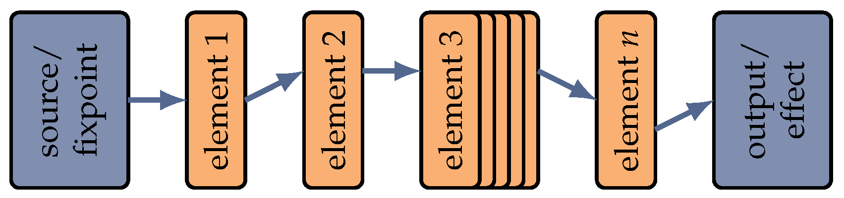
In general, every technical system is a series of a starting point (cause), which might be a source, an input or a fixed point (in any unit), followed by several intermediate elements affecting the physical quantity of the source (targeted as a representation of their function or undesired in the sense of systematic and random errors), leading to an output where the physical quantity comes into effect (Figure 1).

Of course, actual systems are more complex, possibly comprising multiple sources, multiple paths inside the system, and retroaction between elements and multiple outputs.

The approach underlying the proposed method is the vectorial description of the displayed elements, including sources and outputs. There, a flexible data structure and element description is aimed for to ensure a problem- and quantity-independent approach that can easily be adapted, detailed and extended on demand.

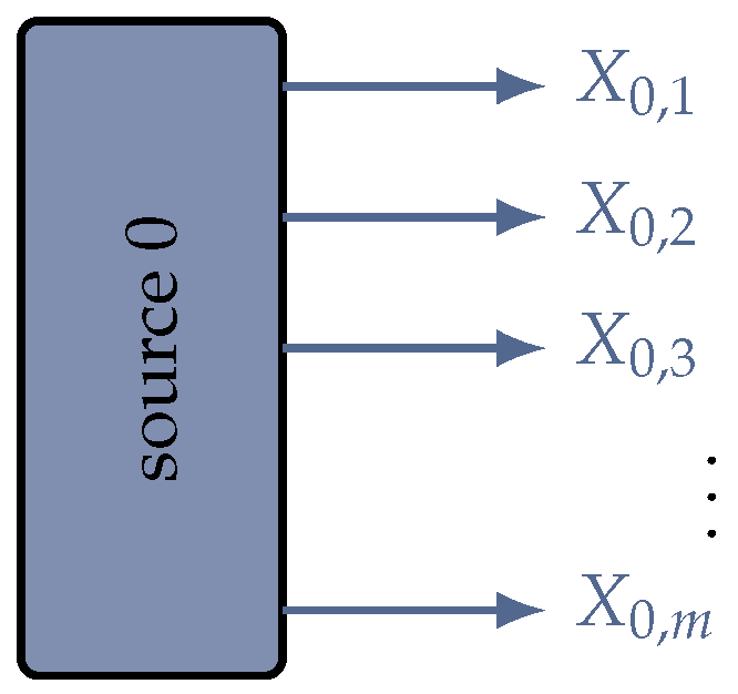
In this method, the source 0 (Figure 2) is the starting point of the data flow in the model. The source is typically a light source, mechanical fixpoint, voltage source or the like; however, it does not necessarily have to be a physical element or body. Notably, it mainly introduces m ($m\in \mathbb{N}$) physical quantities relevant to the physical system, building up the data structure for the following elements. In the first place, the introduced quantities are analytical symbols. The numerical values for evaluation of the specific model are assigned later.

The set of physical quantities provided by the source serves as the input data for the first subsequent element 1. In general, input data are transferred unmodified from the input to the output of each element k (the consecutive number of elements in the model, $k\in \mathbb{N}$). Only the input quantities $X_{ki}$ which are relevant to the respective element k are used, in either a read-only or read–write manner, in the mathematical element model. This is an important detail of the described method, as this entails that the element must be transparent for non-relevant quantities $X_{k,i}$. In this way, the data structure can be designed independent of the number, order and type of elements in the first place. Additionally, the elements need to be modelled only according to the required detail. Quantities $X_{k,i}$ relevant for another sub-set of elements can be neglected during the modelling of elements. Finally, additional or more detailed quantities can later be added to the data stream on demand and at any point, without reprogramming of all existing element models.

Typically, besides the global system model (Equation (1)), the contributions of specific elements needs to be known in detail for inspection and optimisation of the system. For this purpose, the current state of the data structure $X_{k,i}$ can be branched and saved in a snapshot for the observation of local contributions at each intermediate interface (inter-element or intra-element).

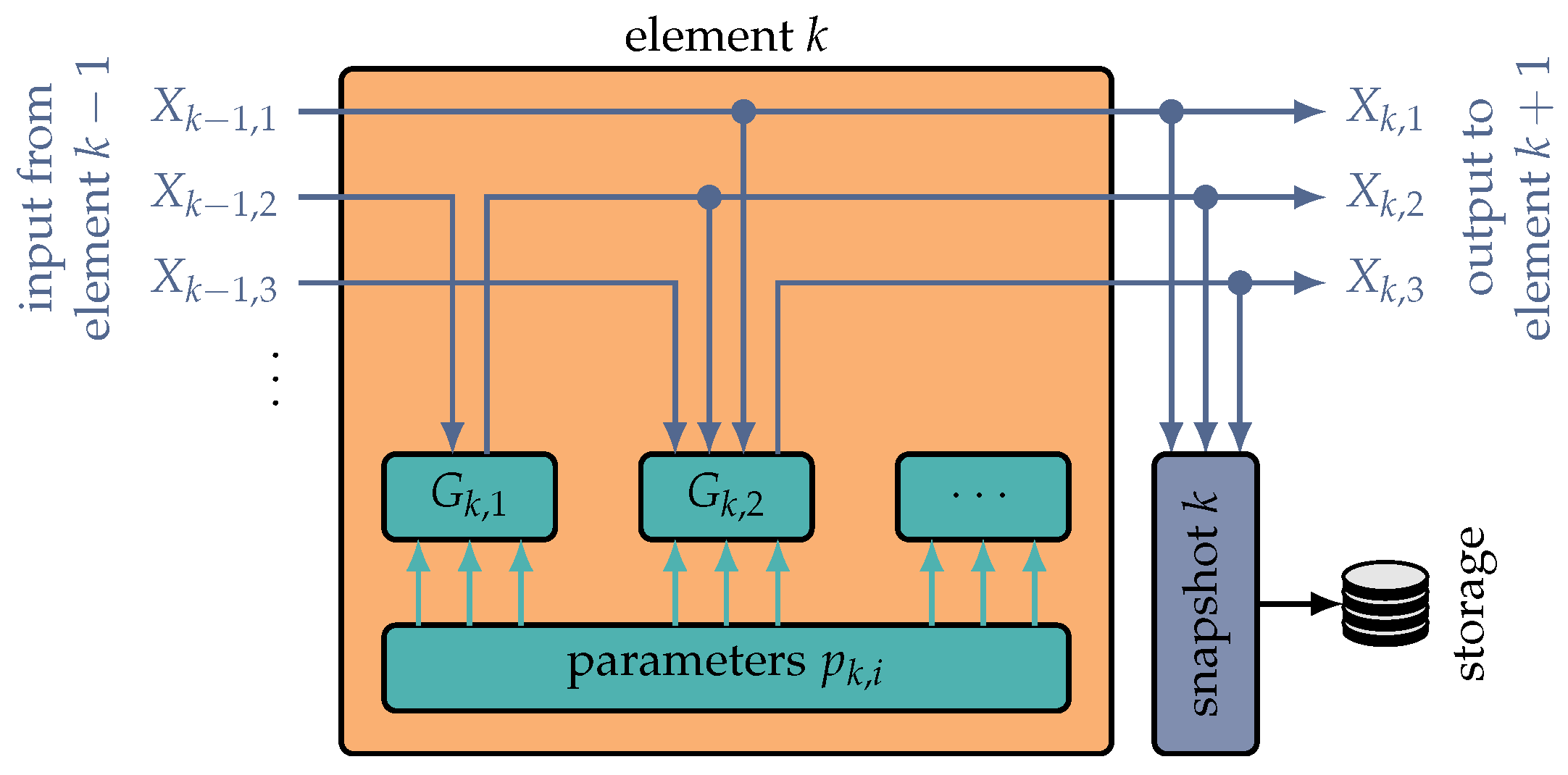
The actual function of each element is modelled in its sub-functions $G_{k,i}$, which can depend on $0\dots n$ input quantities $X_{k-1,i}$ or internal intermediate results and modify $1\dots n$ output quantities $X_{k,i}$ (Figure 3). In each element, the model functions $G_{k,i}$ can be of arbitrary complexity, ranging from a basic physical effect to a combination thereof or even a sub-set of other elements to represent a complex operation. If necessary, $G_{k,i}$ can be added, removed or further detailed on demand.

The output element marks the termination of the data flow in the global model, where the measurand Y is finally calculated based on the other quantities $X_1,X_2,\dots ,X_N$, depending on the parameters $p_{k,i}$ of all preceding elements. With Y now analytically known, the global combined standard uncertainty can be calculated. For this purpose, the output data structure of the last element is processed, according to [3], based on a Taylor series approximation of Equation (1).

In general, the described approach can process scalar and vectorial quantities $X_{k,i}$, as long as the subfunctions $G_{k,i}$ are prepared accordingly. Here, the focus is on describing the system in a vectorial way.

This allows the parameter handling in each element to be global, without the need of local parameter transformations. Based on this, the global parameters of the inter- and intra-element boundaries can be calculated. As the elements are modelled in a vector-based manner as well, these calculations should work as expected. In the method, the parameters of an element can be defined globally fixed (possibly with tolerances), as is typical for optical systems. However, the parameters can also depend on the output of the preceding element, which is useful for modelling mechanical problems (position and orientation of an element depend on the preceding one).

The propagation of the vectorial quantities through the elements and the interconnections is performed by vector tracing. The current state and connections of all elements are defined by the element parameters and the data stream; thus, this propagation can be calculated iteratively between and inside elements. The tracing process of calculating the input and output quantities is repeated until the final element is reached. At each point in this chain, the current quantity $X_{k,i}$ is a function of the previous quantity $X_{k,i-1}$; hence, the model Equation (1) is built up gradually with each boundary k and the respective model function $G_{k,m}$ from the source to the exit.

4. Example

As described above, the proposed method was designed to be capable of handling different physical quantities. In this section, a basic attempt to model optical elements is briefly described. The method makes extensive use of hierarchical nested descriptions of complex structures. Thus, the starting point is the mathematical description of basic physical effects.

In optics, the source (Figure 2) typically represents a light source (e.g., laser), emitting light with different physical quantities $X_{0,i}$ (wavelength, intensity, polarisation, etc.). At each output boundary (inter- or intra-element), the quantities $X_{k,i}$ leave this boundary at distinct points ${\mathit{P}}_{k,i}$ and in distinct directions ${\mathit{S}}_{k,i}$. For optical and similar systems, there are free space beam sections between boundaries. Thus, the input point ${\mathit{P}}_{k+1,i}$ of $X_{k,i}$ at the subsequent boundary $k+1$ is calculated based on the intersection of the line defined by ${\mathit{P}}_{k,i}$, ${\mathit{S}}_{k,i}$ with the boundary surface $k+1$, defined by the global position and orientation of the respective element.

For a plane boundary, ${\mathit{P}}_{k+1,i}$ is calculated by the intersection of the incoming beam ${\mathit{P}}_{k,i}$, ${\mathit{S}}_{k,i}$ with the boundary plane, defined by its normal vector $\mathit{N}$ and an arbitrary point $\mathit{P}$, as an element of the plane [26]:

$$\begin{array}{cc}\hfill {\mathit{P}}_{k+1,i}& ={\mathit{P}}_{k,i}-\left({\displaystyle \frac{\left(\mathit{N}·{\mathit{P}}_{k,i}\right)-\left(\mathit{N}·\mathit{P}\right)}{\mathit{N}·{\mathit{S}}_{k,i}}}\right)·{\mathit{S}}_{k,i}\hfill \end{array}$$

(2)

with the dot product ($·$). A similar approach can be applied applies to other surfaces describable by mathematical functions (e.g., a spherical cap for lenses or curved mirrors).

This equation provides the location of the input point of the boundary $k+1$, which is typically coincident with the output point of the same boundary.

The direction ${\mathit{S}}_{k+1,i}$ of the output beam depends on the type of boundary and the optical effect to be modelled there. For refraction, the mathematical description of the physical effect is the vectorial representation of the Snell–Descartes law [27]:

$$\begin{array}{cc}\hfill n& ={\displaystyle \frac{n_k}{n_{k+1}}}\hfill \\ \hfill {\mathit{S}}_{k+1,i}& =n{\mathit{S}}_{k,i}-\mathit{N}\left(n\left(\mathit{N}·{\mathit{S}}_{k,i}\right)-\sqrt{1-n^2(1-{\left(\mathit{N}·{\mathit{S}}_{k,i}\right)}^2)}\right)\hfill \end{array}$$

(3)

with $\mathit{N}$ being the (possibly local) normal vector of the boundary surface, and $n_k$ and $n_{k+1}$ are the respective refractive indices of the material before and after the boundary.

In a similar way, reflection can be modelled based on the normal vector $\mathit{N}$ of the reflecting surface and the direction ${\mathit{S}}_{k,i}$ of the incident beam [27]:

$$\begin{array}{cc}\hfill {\mathit{S}}_{k+1,i}& ={\mathit{S}}_{k,i}-2\left(\mathit{N}·{\mathit{S}}_{k,i}\right)\mathit{N}\hfill \end{array}$$

(4)

For mechanical and other systems, the input point and direction of the subsequent element may be computed differently, in order to model firm connections, mechanical degrees of freedom, friction, elasticity and so on.

Following this concept throughout all elements, at each point in the chain, the location and direction of the current beam is a function of the previous point and direction:

$${\mathit{P}}_{k+1,i},{\mathit{S}}_{k+1,i}=G_{k,m}({\mathit{P}}_{k,i},{\mathit{S}}_{k,i})$$

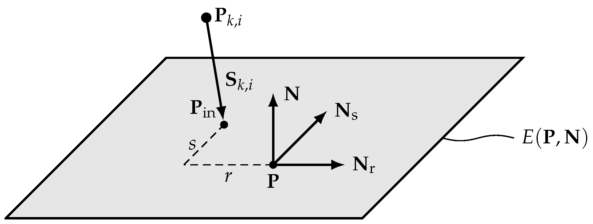
In this way, the model Equation (1) is built up gradually with each boundary k and the respective model function $G_{k,m}$ from the source to the exit of the system. The exit can be either the output data stream of the last element, or a final boundary (i.e., a specimen, screen or detector with its own local coordinate system). The position and orientation of this boundary can also be defined by the user specifying the respective detection plane E (Figure 4).

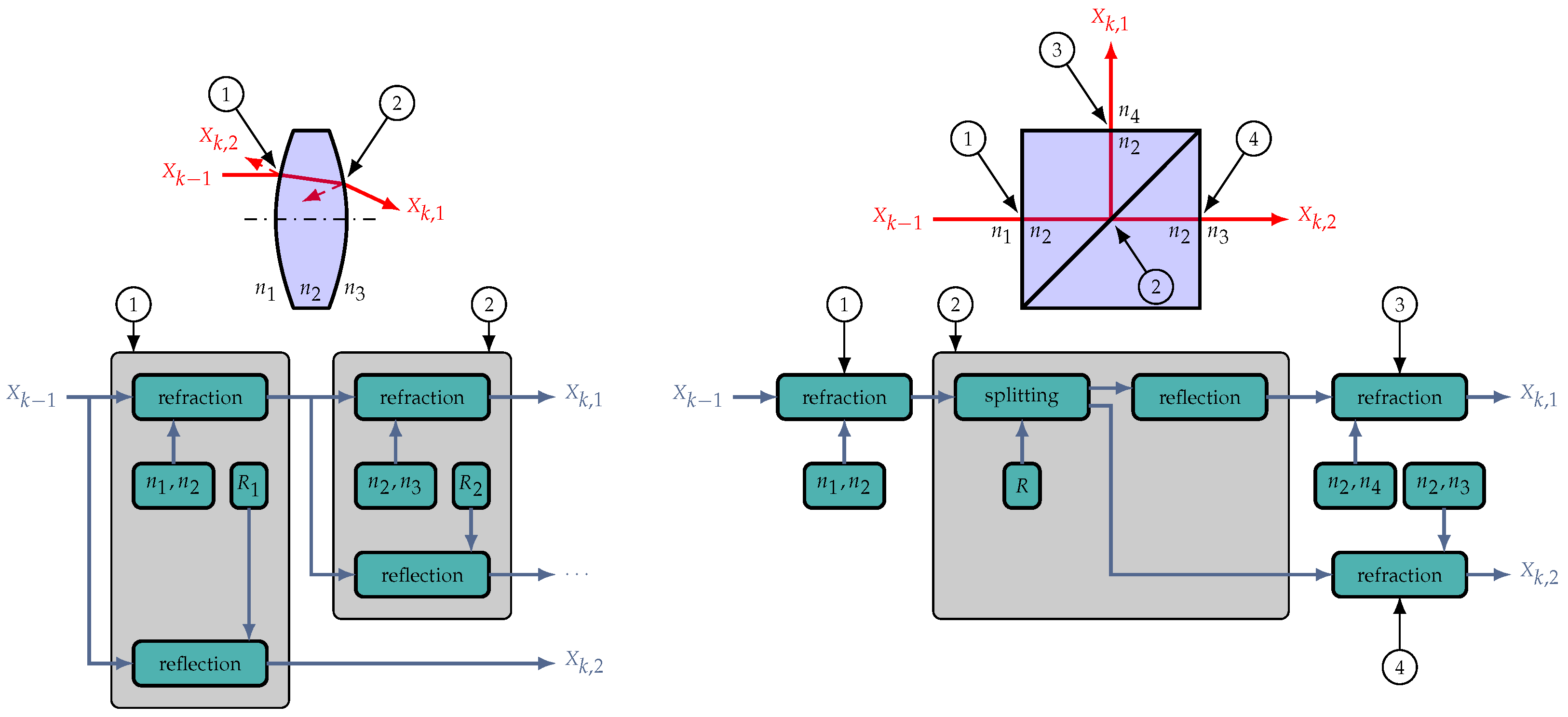
Based on these primary relations, quite complex optical parts can be modelled by defining the positions and orientations of the respective functional surfaces and the composition and appropriate linkage of the underlying sub-functions $G_{k,i}$ (Figure 3); for example, according to Equations (2)–(4). In optics, at every boundary surface, refraction and reflection can be modelled as required, even accounting for parasitic effects (e.g., ghost reflections), if required in the current application. The parameters, positions and orientations of all boundaries can either be fixed, include a tolerance or be subject to the input data stream (e.g., to account for mechanical movement such as the positioning of stages).

These optical parts can then be arranged into optical systems by positioning single parts and appropriate linking. In this way, a hierarchical model can be built from the basic physics up to the complete system.

In the models, optical parameters do not necessarily have to be constant but can depend on other part parameters or on input quantities. This opens up the possibility to model phenomena such as dispersion. For example, by adding a dispersion formula for $n_2$ in the lens model of Figure 5, wavelength-dependent properties can be modelled.

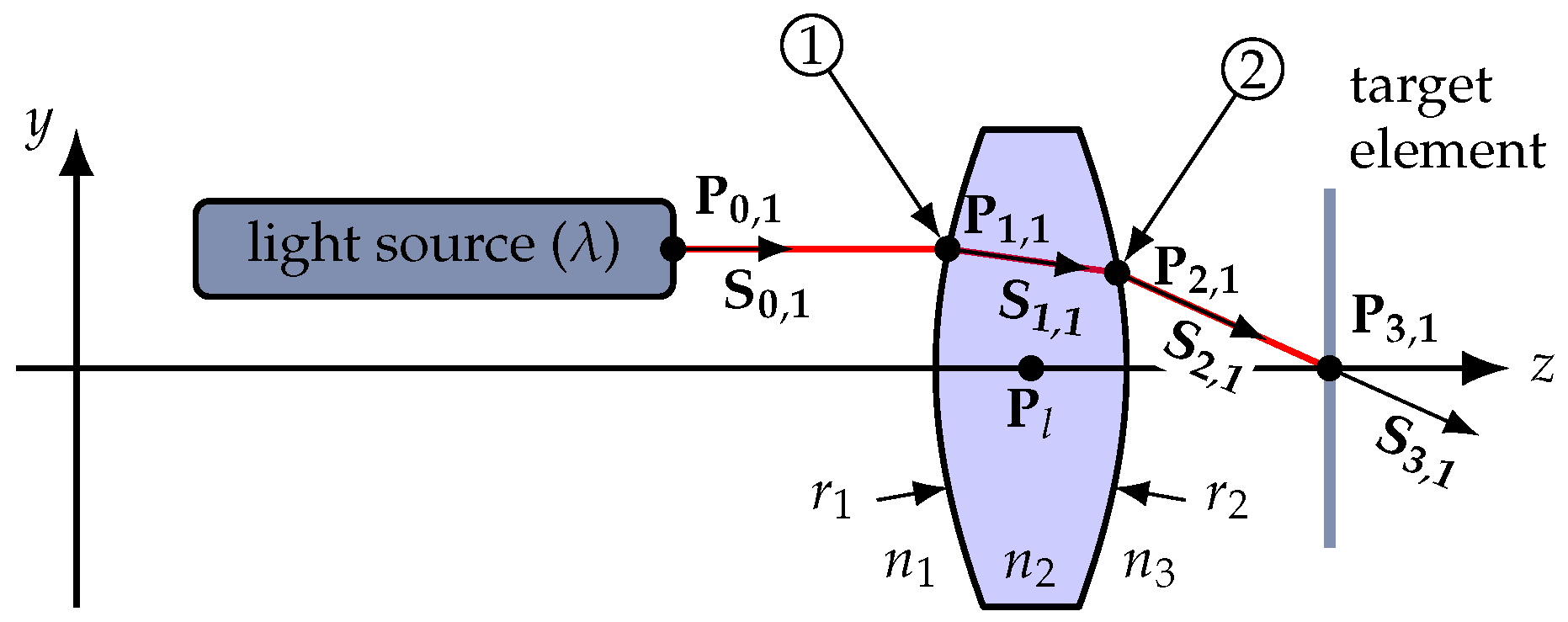
For sake of demonstration, a single spherical lens is modelled according to the setup shown in Figure 6. The example is simplified to describe the process of modelling with the proposed method in a clear manner. Hence, the setup contains an ideal light source emitting a single ray of variable wavelength (source in Figure 1), the lens to be modelled (element 1 in Figure 1) and a detector (output in Figure 1 and Figure 4). The only uncertainty in the system is presumed to be the position of the lens in the y-direction. In this example, the quantity of interest is the angle $\varphi$ of the lens exit ray with respect to the optical axis z.

The light source in Figure 6 also acts as the source of the vectorial model (compare Figure 1 and Figure 2), introducing the quantity vacuum wavelength $(X_{0,1}=\lambda )$ at the position of the light source ${\mathit{P}}_{0,1}$ in the emitting direction of the light source ${\mathit{S}}_{0,1}$.

From the light source, there is a free space beam section until the first air–glass transition at the lens (labelled ➀ in Figure 5 and Figure 6). In an actual calculation, the lens would be modelled as a complex element according to Figure 5, and then abstracted to a black-box only providing inputs, outputs and element parameters (position, orientation, focal length, material etc.) for convenient re-use. In this example, the hierarchical modelling and abstraction processes are discarded for clarity.

The transition at the first air–glass boundary is the sub-function $G_{1,1}$ (compare Figure 3 and Figure 5) of the lens. The entrance point ${\mathit{P}}_{1,1}$ of the ray into the lens surface is calculated by the intersection of the line ${\mathit{P}}_{0,1},{\mathit{S}}_{0,1}$ with a sphere [26] defined by its radius $r_1$ and centre ${\mathit{P}}_s$:

$$\begin{array}{cc}\hfill {\mathit{P}}_{1,1}& ={\mathit{P}}_{0,1}-\left({\mathit{S}}_{0,1}·({\mathit{P}}_{0,1}-{\mathit{P}}_s)+\sqrt{{\left({\mathit{S}}_{0,1}·({\mathit{P}}_{0,1}-{\mathit{P}}_s)\right)}^2-{\Vert {\mathit{P}}_{0,1}-{\mathit{P}}_s\Vert }^2+r_1^2}\right){\mathit{S}}_{0,1}\hfill \end{array}$$

with $\Vert ·\Vert$ denoting the Euclidean norm.

With the entrance point known, the refraction at the boundary is calculated according to Equation (3) using ${\mathit{P}}_{1,1}-{\mathit{P}}_s$ as the local normal vector $\mathit{N}$, resulting in the ray direction ${\mathit{S}}_{1,1}$ inside the lens material. There, the refractive index of the lens material is considered to be wavelength-dependent, according to the dispersion formula for the selected material. One basic concept of the proposed method is that only quantities affected by the current boundary are recalculated (here, this is the vector ${\mathit{S}}_{0,1}$), while other quantities are passed through to the next boundary. In this example, this is the vacuum wavelength $\lambda$, which is not affected by the air–glass transition. The described calculation steps apply in a similar way to the exit surface of the lens ($G_{1,2}$), yielding ${\mathit{P}}_{2,1}$ and ${\mathit{S}}_{2,1}$. At both points ${\mathit{P}}_{1,1}$ and ${\mathit{P}}_{2,1}$, parasitic reflections could be considered as well, using Equation (4) and an appropriate coefficient of reflection. However, in this example, parasitic reflections are omitted. If reflections become an issue, the required steps would be

• adding the quantity intensity $X_{0,2}=I$ to the source (Figure 2)
• programming a lens model including reflection;

  (a)

  adding Equation (4) as additional $G_{k,i}$ to both surfaces of the lens;

  (b)

  adding the parameter coefficient of reflection $p_{k,i}=R$ to the lens model;

  (c)

  adding the modification of I according to R at each surface;

  (d)

  adding two outputs to the lens model;

• replacing the old lens model with the extended one;
• adding I to the evaluation.

From then on, both models can be used interchangeably depending on the requirements, without the need for reprogramming of other elements.

Finally, the intersection of the ray with the target element is calculated according to Equation (2) (sub-function $G_{2,1}$), yielding ${\mathit{P}}_{3,1}$ and ${\mathit{S}}_{3,1}={\mathit{S}}_{2,1}$. There, the quantity of interest—the angle $\varphi$ of ${\mathit{S}}_{3,1}$ with respect to the normal vector ${\mathit{N}}_{\mathit{t}}$ of the target element—is calculated [26]

$$\varphi =arccos\left({\displaystyle \frac{{\mathit{S}}_{3,1}·{\mathit{N}}_{\mathit{t}}}{\Vert {\mathit{S}}_{3,1}\Vert \Vert {\mathit{N}}_{\mathit{t}}\Vert }}\right).$$

(5)

In this way, the model function f is built up iteratively from the source to the target element:

$$f=\varphi =G_{2,1}\left(G_{1,2}\left(G_{1,1}\left({\mathit{P}}_{0,1},{\mathit{S}}_{0,1},n_1,n_2\left(\lambda \right),r_1,{\mathit{P}}_s\right),n_2\left(\lambda \right),n_3,r_2,{\mathit{P}}_s\right),{\mathit{N}}_{\mathit{t}}\right)$$

(6)

Once f is known, the uncertainty evaluation as described in GUM can be carried out as usual, calculating the sensitivities $c_i=\partial f/\partial X_i$ and propagating the probability density functions of the $X_i$ through the model. As all $G_{k,i}$ are analytic functions, and the vector calculations are processed analytically as well, f is obtained as an exact equation, purely formulated in variables ($r_1$, $n_2$ etc.), without numerical estimations. However, f and the $c_i$ are not displayed in full detail here as, even for this simple example, they are extensive equations. In the early state of system design, this enables a sophisticated and flexible analysis allowing for the design, optimisation and implementation of control systems for the modelled construct. Furthermore, for more complex systems, the exact formulation of f and $\partial f/\partial X_i$ allows for the systematic identification of reasonable actuator positions, parameters and manufacturing tolerances and, hence, optimisation of the system structure itself.

When the design process becomes more specific, the $X_i$ in can be replaced by their respective estimates $x_i$ in f and $\partial f/\partial X_i$. In this example, this step is performed for comparison of the proposed vectorial method with a reference simulation. For this purpose, the system shown in Figure 6 is calculated for the numerical parameters in

Table 1. Numerical parameters for the optical system in Figure 6. Coordinates are in $(y,z)$. For clarity, the only uncertainty in the system is assumed to be the lens position ${\mathit{P}}_l$ in this example, while all other input quantities $x_i$ are considered to have zero uncertainty.

Part	Parameter	Value
light source	$\lambda$ range	300–2400 nm
	${\mathit{P}}_{0,1}$	($1.9$ $\mathrm{m}$$\mathrm{m}$, $-10$ $\mathrm{m}$$\mathrm{m}$)
	${\mathit{S}}_{0,1}$	(0, 1)
lens	${\mathit{P}}_l$	(0, 0)
	$u\left({\mathit{P}}_l\right)$	(50 $\mu$$\mathrm{m}$, 0)
	opt. axis	(0, 1)
	$r_1=r_2$	$10.302$   $\mathrm{m}$$\mathrm{m}$
	centre thickness	2  $\mathrm{m}$$\mathrm{m}$
	material	N-BK7, dispersion data $n_2\left(\lambda \right)$ from [28]
	$n_1=n_3$	1.0
target element	position	(0, 10 $\mathrm{m}$$\mathrm{m}$)
	surface normal vector	(0, −1)

.

The numerical results of $\varphi \left(\lambda \right)$ and $u\left(\varphi \right)$ for the parameters given in Table 1 are plotted in Figure 7, in which the expected effect of dispersion on $\varphi$ can be seen. Less obviously, the wavelength-independent mechanical tolerance of the lens position $u\left({\mathit{P}}_l\right)$ (Table 1) results in a wavelength-dependent uncertainty $u\left(\varphi \right)$. This indicates that sources of uncertainty can be identified in good detail with the proposed method, opening the opportunity for sound analysis of complex systems. To validate the results, the same optical setup was modelled in a commercial optical CAD software (Quadoa v25.04 [29]). Simulations were carried out numerically for discrete wavelengths, marked as dots in Figure 7. The respective position uncertainty $u\left({\mathit{P}}_l\right)$ was accounted for by a 50 $\mu$$\mathrm{m}$ shift of the lens in the y-direction and calculating the combined standard uncertainty numerically according to GUM.

The plot shown in Figure 7 indicates the good agreement between the proposed method and commercial simulation software, hence demonstrating the reliability of the basic concept. Of course, correct modelling of the single physical effects and elements is essential. However, the hierarchical approach enables a convenient work flow for modelling, debugging and reuse of code blocks.

The example setup was intentionally kept simple to focus on the structure and the process of the vectorial model. The calculations here could well be performed manually with plane trigonometry. However, extending the lens tolerance $u\left({\mathit{P}}_l\right)$ to the third dimension x (not shown in Figure 6) would already complicate the calculations enormously, demonstrating the advantage of the vectorial approach. Of course, more complex calculations can also be carried out. For example, polarisation calculations can be added to the model through defining additional vectors orthogonal to the vectors $\mathit{S}$, representing the amplitude and phase of the respective electrical field.

Once again, the described method can also be applied to other physical quantities, allowing complex scenarios to be described as a combination of the basic underlying physical effects.

5. Conclusions

Evaluating and expressing uncertainty in measurements is required in a broad spectrum of applications in science, engineering and industry, in order to quantify the quality of a measurement result and assess its reliability. Although the process and method defined with GUM is universal, consistent and transferable, setting up the mathematical model of a measurement process can become a complex task even for moderate setups. The method proposed in this contribution is based on a vectorial approach for systematic and flexible modelling. The division of the complex problem into sub-elements that can be modelled in a self-contained manner helps to keep track of the system structure, and vectorial modelling releases the user from cumbersome in-plane mathematical descriptions of three-dimensional geometric problems. The data structure was aimed to be flexible and extensible, allowing for the inclusion of further levels of detail as the measuring setups and their corresponding models evolve. As the proposed method allows for a consistent analytical description of the measurement process, it can provide an efficient analytical calculation of the partial derivatives required for the sensitivity coefficients of the Taylor series approximation. In the considered example, the method was described in detail and the results were in accordance with a numerical simulation of the same example using commercial optical CAD software. Although the method was originally developed for system design in optical imaging, the underlying concept is also suitable for systems and measurements comprising physical quantities other than optical ones.