SurfILE: An Open-Source Python Package for Surface Topography Analysis

Abstract

Surface metrology deals with inspecting surfaces and profiles by using contact or non-contact profilometers. In this field, the characterization of the dimensional, morphological, and texture parameters of samples as well as the assessment of metrological characteristics of measuring instruments are key issues. Manufacturers of instruments provide commercial software tools to analyze topography data. There are also freely available tools, including open-source options, that provide a variety of algorithms and methods. The rapid growth of investigations aimed at better understanding the effects of the microscale phenomena requires the improved traceable calibration of samples, the development of new methodologies and measuring techniques, and the specification of new mathematical models and processing techniques. In this work, we present SurfILE, the launch of an open-source Python project that provides various procedures and algorithms for topography analysis. The open-source software presented in this article is intended to be modular, expandable, and customizable.

1. Introduction

Surface metrology relates to the characterization of surface texture and topographies at the micrometer scale down to the nanometer scale on samples from different areas, such as the automotive and semiconductor industries, healthcare, tribology, etc. This characterization can be achieved using tactile profilometers, microscopes, and optical instruments [1]. Data analysis procedures are used to characterize both the measurand and the instrument itself, and over the last decades, numerous software were released to facilitate the processing of the data collected by the instruments.

In 2002, Sacerdotti et al. started an open-source project to provide for surface texture and topography analysis algorithms: SCOUT—Surface Characterization Open-Source Universal Toolbox [2]. The Matlab^® code was placed on a server at the University of Birmingham, but all maintenance stopped and the codes and the server disappeared.

In the context of metrology at the nanometer and atomic scales using atomic force microscopy and electron microscopy, the Czech national metrology institute (CMI) conducts a powerful open-source project called Gwyddion [3]. Since 2011, this software has been widely used in the field of scanning probe microscopy [3,4], as well as for analyzing surface texture and metrological tasks at the micrometer scale. Over the past decade, the range of functions has been expanded to include standardized analysis procedures that are relevant to surface metrology [5]. The open-source software is implemented in C and comes with a user-friendly interface running on MS Windows, Mac OS X, and various Linux platforms.

Graphical user interfaces (GUIs) facilitate the use of program functions and are advantageous for analyzing a few parameters on a limited set of images [6]. However, GUI becomes impractical when the same parameter has to be analyzed from a batch of hundreds of images with similar shapes but different quantitative characteristics. Some graphics software try to overcome this issue by implementing templates that can be applied to a large number of different files. These templates are often not generic enough to fit files that differ too much from the one used to create the template, resulting in errors or incorrect results.

During the round-robin project of European national metrology institutes titled “EURAMET—Project No 1242 Measurement of Areal Roughness by Optical Microscopes” [7], which began in April 2017, a significant amount of data were collected. The data consisted of many repetitive measurements that required automated batch processing. The comparison was conducted at two levels: first, each partner analyzed their measurement data using their common practices, which may result in differences in the results not only from the measurement process but also from the analysis method. Secondly, the pilot laboratory processed the data of all partners using identical software. To compensate for the lack of batch processing in distributed software, an automated analysis tool within the Python2 framework was developed for this task.

As part of the EMPIR joint research project “20IND07 TracOptic Traceable industrial 3D roughness and dimensional measurement using optical 3D microscopy and optical distance sensors” [8], the Italian national metrology institute, Istituto Nazionale di Ricerca Metrologica (INRiM) has also developed an automatically running analysis tool based on Python, setting up the Python project according to modern object-oriented Python3 standards. Some of the methods and algorithms developed for the 2017 project have been included in INRiM’s software package, initiating an open-source project on GitHub [9]. The presented open-source project is named SurfILE, an acronym that stands for Surf-ace and prof-ILE analysis.

SurfILE may not be as powerful and extensive as Gwyddion, but it provides a collection of code that is ideal for beginners, such as graduate or PhD students, or scientists who need to quickly analyze non-standard tasks. Users can modify existing methods or add their own functions, methods, and classes. This is made possible since the open-source software offers the possibility to directly examine the source code, which is documented in detail in the Python docstrings. Moreover, using the pdoc package, the documentation is easy to read in html format.

For research purposes, this is an advantage compared to proprietary software algorithms, which are often distributed as undisclosed black boxes or with non-detailed documentation. The analysis of surface characteristics is a critical aspect of various scientific and industrial applications, yet there remains a notable lack of dedicated Python packages specifically designed for this purpose. The package is particularly relevant in the context of research and can also be used in the framework of Industry 4.0 to automate the processing of hundreds of topographies and profiles. SurfILE features comprehensive documentation to support users in navigating its functionalities.

Since 2008, the open-source project culture has been given an infrastructure with GitHub [9], a developer platform for creating, storing, managing, and sharing code. To ensure the permanent storage of additional data coming with a publication and being froze to the state when published, open-access repositories (OARs) with unique DOI numbers are available. The current version of the approved topography data analysis algorithms presented in this article are deposited in the OAR with the DOI https://doi.org/10.5281/zenodo.10727546; the GitHub repository of this project contains the entire package, which is in a continuous development process.

2. Package Overview

In order to measure the dimensional or geometric parameters of surface features in a traceable way, it is necessary to characterize the measuring instruments for their metrological capabilities and to calibrate them. Typically, measurement standards are used to determine scale factors, linearity, resolution, and transfer characteristics, which are referred to as “metrological characteristics”, as reported in ISO 25178-600:2019 [10]. In texture analysis, integral statistical quantities such as the root mean square roughness $R_{\mathrm{q}}$ are denoted as “surface texture parameters” [11]. In health science, biology, archaeology, nanometrology, and machine vision, parameters characterizing structures that are not necessarily parameterizable with simple geometric models are called “shape or morphology of features” or “morphological parameters” [12].

Several investigations have been conducted to comprehend the measurement process and physical effects that result in unintended artifacts. This was achieved by simulating confocal microscopes [13] and scanning coherence microscopes [14,15] and comparing simulation results with measurements. Giusca et al. and Leach et al. provide an overview of the measurement methods used to determine various metrological characteristics of optical microscopes with deterministic topographic structures represented by material measurement standards by using the commercial software MountainsMap ${9.3}^{\circledR }$ [16,17,18,19].

The diverse nature of the samples led to the development of different algorithms, each suited for a specific purpose. As an example, the first step in a surface processing pipeline is form removal; SurfILE provides polynomial, spherical, and cylindrical least square fitting, with the option to define methods to set boundaries on the selection of the points used for the fit operation. These methods are explained in Section 3.1.

For over two decades, investigations have been conducted on the response and fidelity of the topography data delivered by optical instruments. In 2010, Leach and Haitjema stated that the resolution of a topography measurement is determined by the ability to measure the spacing of points and accurately determine the heights of features [20]. They also note that the instrument numerical aperture (NA) of the objective sets the limit of detectable slopes and that spikes and overshoots may be observed. In the package, a routine for a maximum measurable slope calculation was implemented, and it is presented in Section 3.2.4.

Important tools for surface processing are slope distributions and PSD. They can be used, respectively, to understand the orientation of the measured sample in both polar angles and the wavelength components in both x and y directions. These routines are implemented in SurfILE and are explained in Section 3.2.1 and Section 3.2.2.

When using tactile profilometers to calibrate measurement standards and provide reference data, the geometry may be distorted based on the size of the probe tip [21]. Morphological filtration is used to mitigate this effect. In 2012, Lou presented three different algorithms to expand the already existing erosion and motif combination routines [22,23]. In 2019, Pawlus introduced the calculation of the structuring element radius for two-process (stratified) profiles [24], and in 2024, Zakharov combined different nesting index filters to implement asymmetric filtration [25]. In this package, an algorithm was implemented as a utility function to perform the morphological operation of erosion, and it is explained in Section 3.3.1.

In surface metrology, it is often required to analyze samples wider than the field of view of the optical instrument. To overcome this issue, stitching can be applied to multiple topographies. In 2007, Marinello proposed an algorithm based on the cross-correlation of images overlap [26], while in 2016, Zhou introduced an algorithm for point cloud registration [27]. Two completely different algorithms, based on these two contributions, have been implemented in SurfILE and are presented in Section 3.3.2.

Package Structure

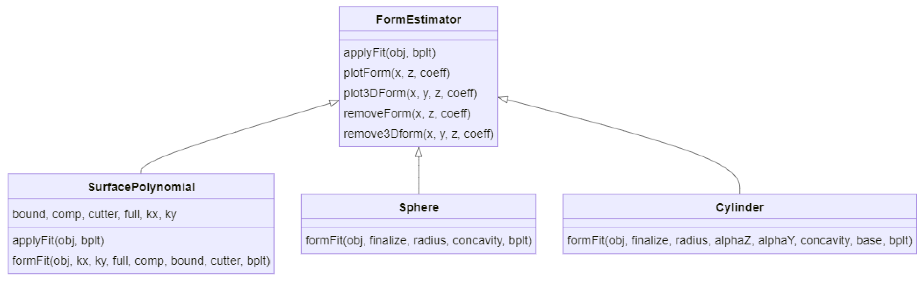
The Python package contains several modules, shown in Figure 1.

The methods and classes can be divided into four categories:

• Data structures: classes that store surface and profile data and handle input/output file operations to open the most common file types from the instrument manufacturers (Figure 2);

• Form operators: methods for surface and profile leveling and form fitting (Figure 3);

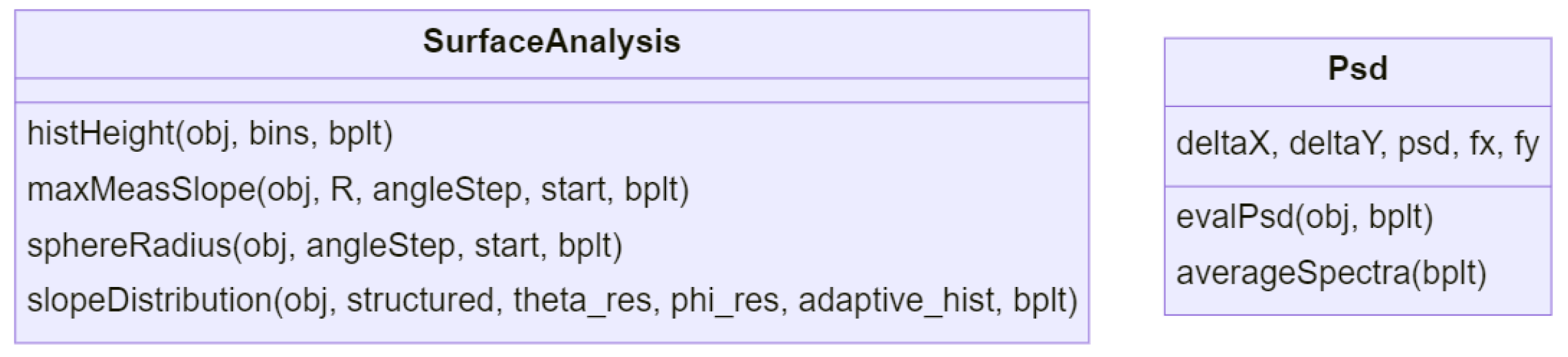
• Processing: methods for surface and profile analysis to extract morphological parameters or metrological characteristics (Figure 4);

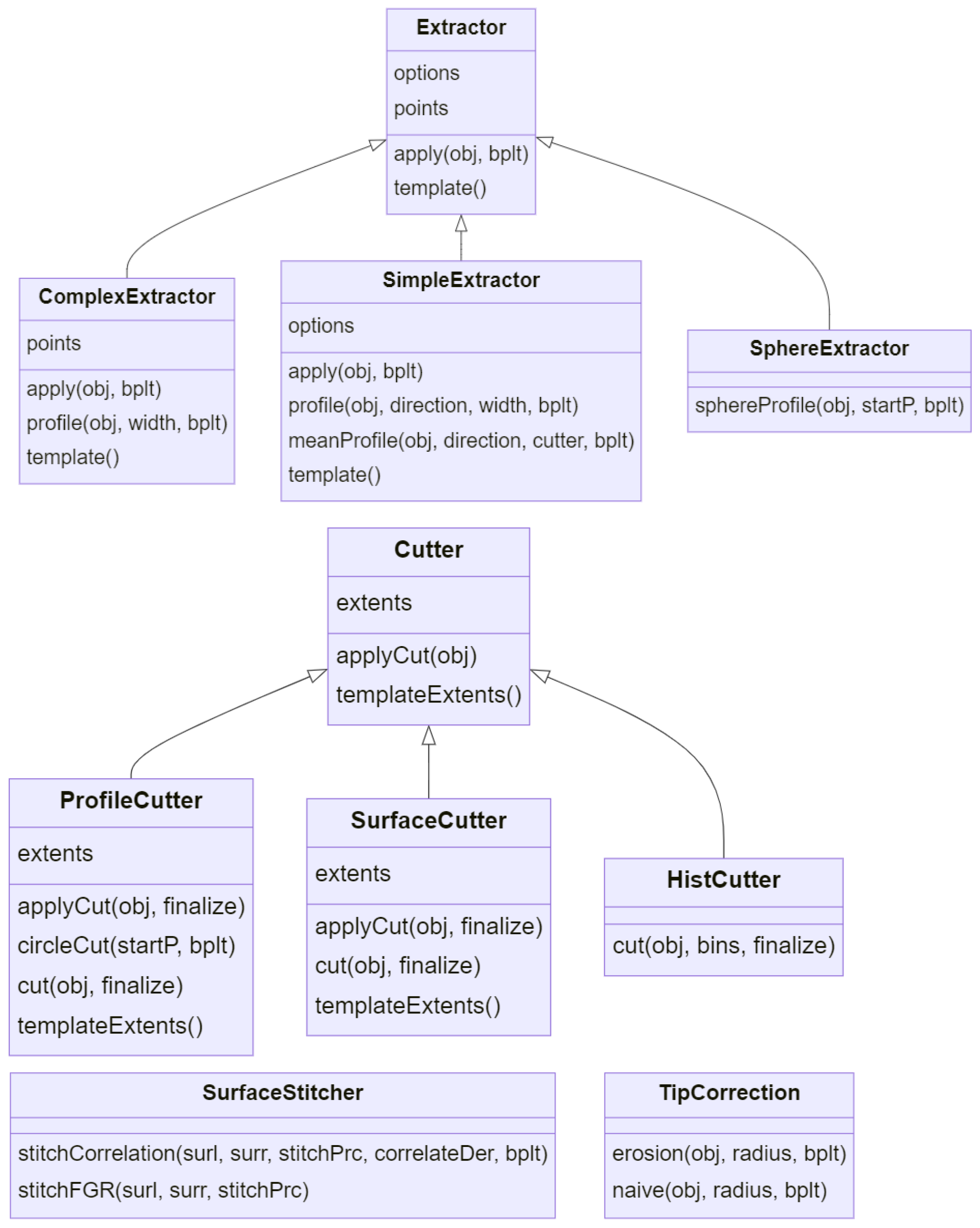
• Utilities: stitching routines, profile extractors, and simple cutter objects (Figure 5).

The package can be easily expanded and further functionality can be implemented in the modules while maintaining readability and simplicity in the code structure.

3. Materials and Methods

3.1. Form Operators

The form or geometry parameters are estimated by minimizing the sum of the squares of the residuals ${\epsilon }_i$ of $i=0,\dots ,n-1$ data points (Equation (1)):

$${\epsilon }_i=f(\mathbf{p},x_i,y_i,z_i)$$

(1)

where $(x_i,y_i)$ are the sampling positions, $z_i=z(x_i,y_i)$ are the height values of the topography map, f is the model function, and $\mathbf{p}=[p_0,p_1,\dots ,p_m]$ is the tuple of geometry parameters or polynomial coefficients to be estimated by optimization (Equation (2)):

$$\underset{\mathbf{p}}{min}\left\{\sum _{i=0}^{n-1}f{(\mathbf{p},x_i,y_i,z_i)}^2\right\}$$

(2)

If an explicit representation of z as a function of x and y is possible (Equation (3)),

$$z_i=z(\mathbf{p},x_i,y_i)+{\epsilon }_i\hookrightarrow \underset{\mathbf{p}}{min}\left\{\sum _{i=0}^{n-1}{\left(z_i-z(\mathbf{p},x_i,y_i)\right)}^2\right\}$$

(3)

the library functions leastsq of scipy.optimize wrapping the MINPACK library [28] or lstsq of numpy.linalg can be used.

Once the geometry of a feature has been determined, further processing of the residual topography after form removal can also be carried out to characterize form deviations and to characterize parameters such as the power spectral density; in the package, all the form operators are collected in the geometry.py module.

3.1.1. Polynomials

For complex geometries, it is often necessary to fit the data points with a polynomial surface of degree $k_x$ and $k_y$, and this is implemented in the method SurfacePolynomial.formFit. The solution of the polynomial fit is matrix $\mathbf{M}$ in Equation (4):

$$\begin{array}{c}\mathbf{M}=\left[\begin{array}{ccc}{m}_{0,0}& \cdots & m_{0,k_x}\\ ⋮& \ddots & ⋮\\ m_{k_y,0}& \cdots & m_{k_x,k_y}\end{array}\right]\end{array}$$

(4)

The elements marked in red in Equation (4) represent the lower-right triangle that can be discarded or considered in the polynomial Equation (5):

$$z_{\mathrm{poly}}(x,y)=\sum _{i,j}{m}_{i,j}·x^i·y^j$$

(5)

By removing the calculated polynomial from the original topography, it is possible to obtain the form removal operation of Equation (6):

$$z_{\mathrm{form}\_\mathrm{removed}}(x,y)=z(x,y)-z_{\mathrm{poly}}(x,y)$$

(6)

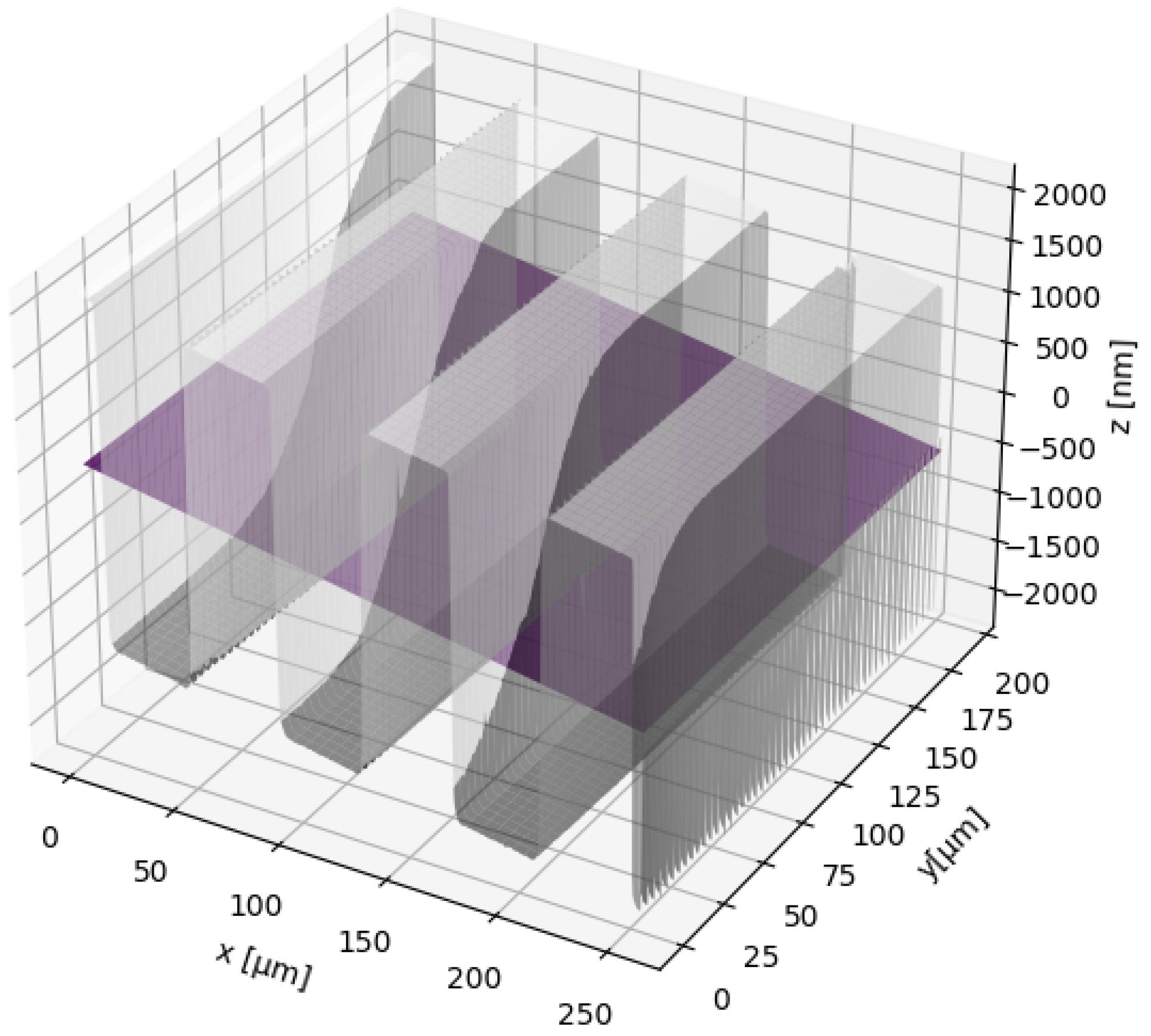
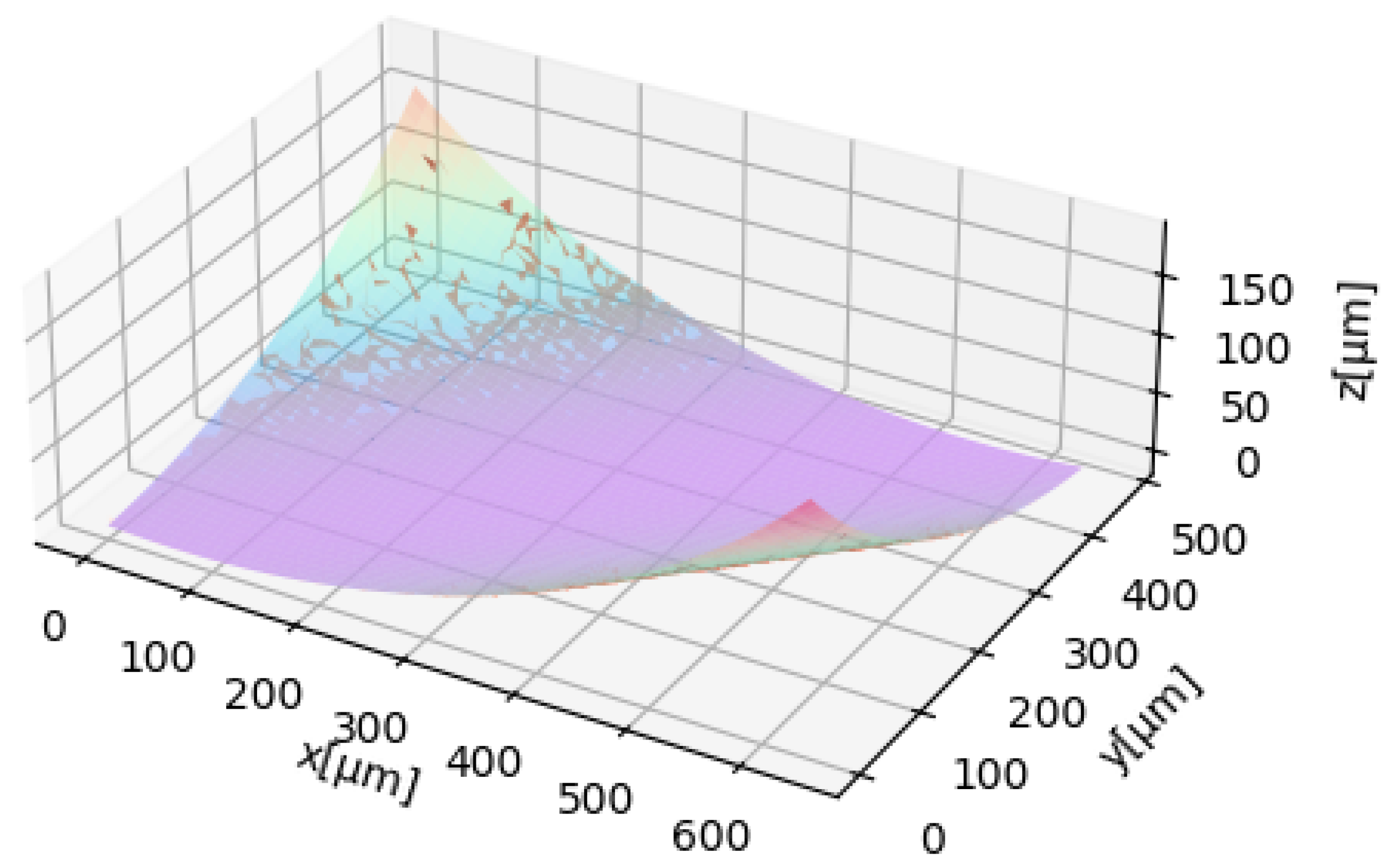
When leveling topographies that are periodic and symmetrical with respect to a horizontal plane, the least squares leveling method may fail. To overcome this problem, the fit can be performed on a restricted set of points, as shown in Figure 6. The user can select these points by setting three parameters:

• Bound: threshold height (if the height is not specified by the user, it is automatically considered equal to the mean value of the topography);
• Comp—lambda expression: a condition that specifies whether to consider points above or below the threshold;
• Cutter: the evaluation area is cut from the measurement area according to the region of interest in the $XY$ plane.

Figure 6. First- degree polynomial fit (purple plane) on RSM-3 grating structure (gray topography) with threshold point exclusion.

Figure 6. First- degree polynomial fit (purple plane) on RSM-3 grating structure (gray topography) with threshold point exclusion.

3.1.2. Cylinders

This fit algorithm implemented in Cylinder.formFit is developed for the processing of a cylindrical feature. To extract roughness parameters or other features, it is necessary to remove the primary form of the surface. Numerous algorithms are present in the literature but are all based on cylindrical coordinates [29]. The general Equation of a cylinder is reported in Equation (7):

$${(x-x_c)}^2+{(y-y_c)}^2+{(z-z_c)}^2-{[l(x-x_c)+m(y-y_c)+n(z_{\mathit{cyl}}-z_c)]}^2-R^2=0$$

(7)

where $x,y,z_{\mathit{cyl}}$ are the coordinates of the cylinder points; $l,m,$ and n are the three components of the versor that represent the cylinder axis direction; $x_c,y_c$, and $z_c$ are the coordinates of the center; and R is the radius of the circular base.

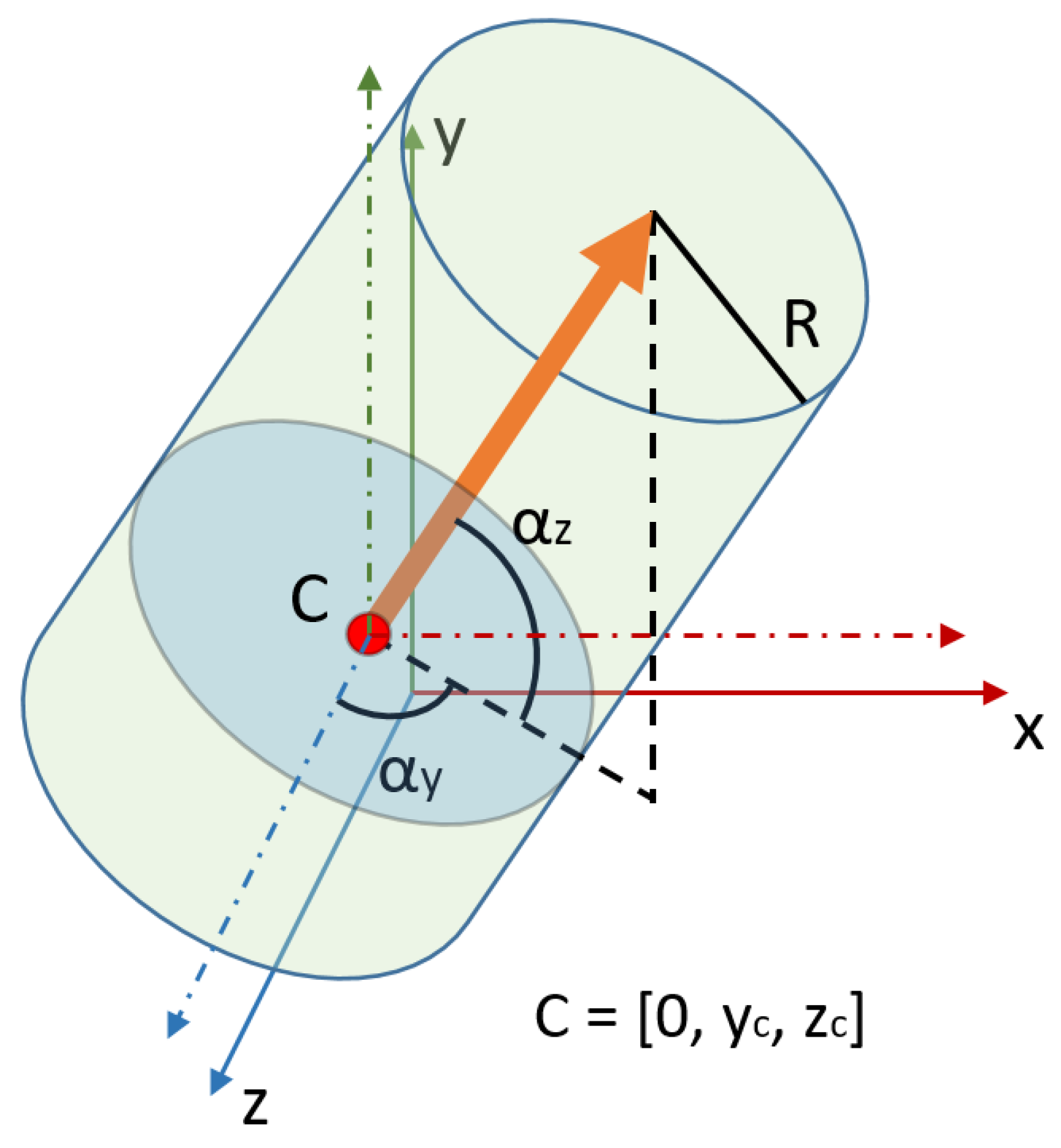
Since a cylinder in 3D space has five degrees of freedom (Figure 7) and the above equation has seven undefined parameters, we need to find a different equation with five parameters independent of each other. To achieve this, two initial considerations are needed:

• The cylindrical features are assumed to always be measured with the axis lying on the $YZ$ plane $(x_c=0)$. Note that this assumption does not limit the orientation of the cylinder since we could have chosen any of the three center coordinates to be zero.
• The versor components $l,m,$ and n (Equation (8)) can be derived from the feature angles elevation $\left({\alpha }_z\right)$ and rotation $\left({\alpha }_y\right)$, thus reducing the parameters from three to two:

$$\begin{array}{c}l=cos\left({\alpha }_z\right)cos\left({\alpha }_y\right)\\ m=sin\left({\alpha }_z\right)\\ n=cos\left({\alpha }_z\right)sin\left({\alpha }_y\right)\end{array}$$

(8)

Using a Python optimization tool from the SciPy library, the program calculates the best estimates for the five parameters using the least square method in Equation (9) and then calculates the cylinder points and subtracts them from the surface:

$$\underset{\mathbf{p}}{min}\left\{\sum _{i=0}^{n-1}{[z_i(x,y)-z_{cyl,i}(\mathbf{p},x,y)]}^2\right\}$$

(9)

where $\mathbf{p}$ is the tuple of all the cylinder parameters (Equation (10)):

$$\mathbf{p}=[R,{\alpha }_y,{\alpha }_z,y_c,z_c]$$

(10)

Rewriting the cylinder equation and substituting $t=z_{cyl}-z_c$, we obtain Equation (11).

$$x^2+{(y-y_c)}^2+t^2-{[lx+m(y-y_c)+nt]}^2-R^2=0$$

(11)

Equation (11) can be written as a second-degree equation (Equation (12)):

$$A{t}^2+Bt+C=0$$

(12)

where A, B, and C are reported in Equation (13):

$$\begin{array}{c}A=1-n^2\\ B=-2n[lx+m(y-y_c)]\\ C=(1-l^2)x^2+(1-m^2){(y-y_c)}^2-2xlm(y-y_c)-R^2\end{array}$$

(13)

By solving Equation (12), two possible solutions representing the convex or concave fitted cylinder can be obtained. These cylinders can be subtracted from the topography to remove the primary form, as shown in Equation (14):

$$z_{\mathrm{cyl}\_\mathrm{removed}}(x,y)=z(x,y)-z_{cyl}(x,y)$$

(14)

The result of the fit of a cylindrical feature is reported in Figure 8:

Figure 7. Five degrees of freedom cylinder with $R,{\alpha }_y,{\alpha }_z,y_c,z_c$ independent parameters.

Figure 7. Five degrees of freedom cylinder with $R,{\alpha }_y,{\alpha }_z,y_c,z_c$ independent parameters.

3.1.3. Spheres

The program, with the method Sphere.formFit, allows for the removal of the best-fit sphere from a topography. Furthermore, it also calculates the center position and the radius of the sphere. The method used is the least square sphere (LSS) method presented in [30] and adapted to a more parallelizable matrix form as explained in [31] to allow for the implementation with the scipy.linalg.lstsq routine.

The general equation of a sphere is reported in Equation (15), where r is the radius and $x_c$, $y_c$, and $z_c$ are the center coordinates:

$${(x-x_c)}^2+{(y-y_c)}^2+{(z-z_c)}^2=r^2$$

(15)

Expanding the equation, we obtain Equation (16):

$$x^2+y^2+z^2=2x{x}_c+2y{y}_c+2z{z}_c+r^2-x_c^2-y_c^2-z_c^2$$

(16)

Since we are interested in calculating the best $r,x_c,y_c,z_c$ that fit the measured points, we need to express the equation in matrix form according to Equations (17)–(19):

$$\mathbf{f}=\left[\begin{array}{c}{x}_i^2+y_i^2+z_i^2\\ ⋮\\ x_n^2+y_n^2+z_n^2\end{array}\right]$$

(17)

$$\mathbf{A}=\left[\begin{array}{cccc}2x_i& 2y_i& 2z_i& 1\\ ⋮& ⋮& ⋮& ⋮\\ 2x_n& 2y_n& 2z_n& 1\end{array}\right]$$

(18)

$$\mathbf{c}=\left[\begin{array}{c}{x}_c\\ y_c\\ z_c\\ r^2-x_c^2-y_c^2-z_c^2\end{array}\right]$$

(19)

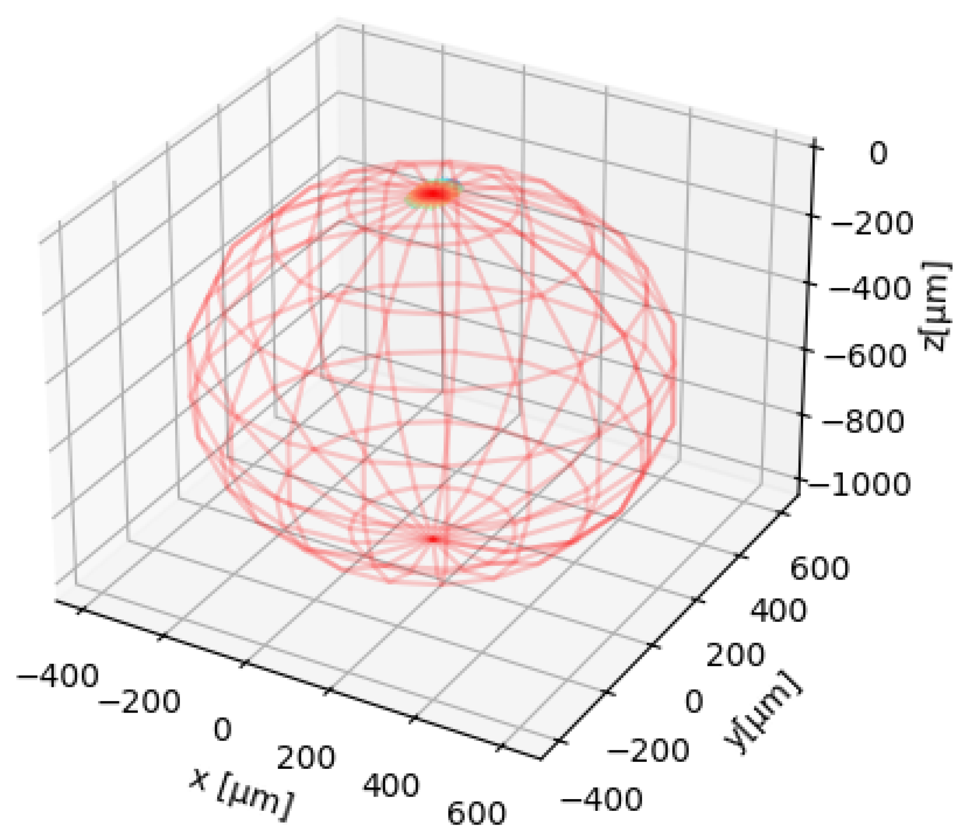
We can now express the equation as $f=Ac$ and then compute the vector $\mathbf{c}$ that minimizes the 2-norm $|f-Ac|$ using the scipy.linalg.lstsq method to find the best values for the four parameters of interest. The fit result is reported in the wireframe plot in Figure 9.

3.2. Data Processing

3.2.1. Slope Distributions

In module texture.py, the method slopeDistribution calculates all the normal vectors to the triangles constructed on the adjacent points of the topography to perform a slope distribution analysis on the surface. The normal vectors are then expressed in polar coordinates, as shown in Figure 10, and for the two angles (elevation $\theta$ and azimuth $\varphi$), a histogram plot is generated.

The number of bins for each angle can be specified by the user by setting two parameters of the calculation:

• Angular resolution: the angle step used to create the histogram, or the bin width.
• Adaptive histogram: If this parameter is disabled, the program will create the histogram considering a span of 0–${90}^{\circ }$ for the angle $\theta$ and a span of 0–${360}^{\circ }$ for the angle $\varphi$. If instead the parameter is enabled, the histogram will span from $0^{\circ }$ to the maximum angle reached by the calculated distribution.

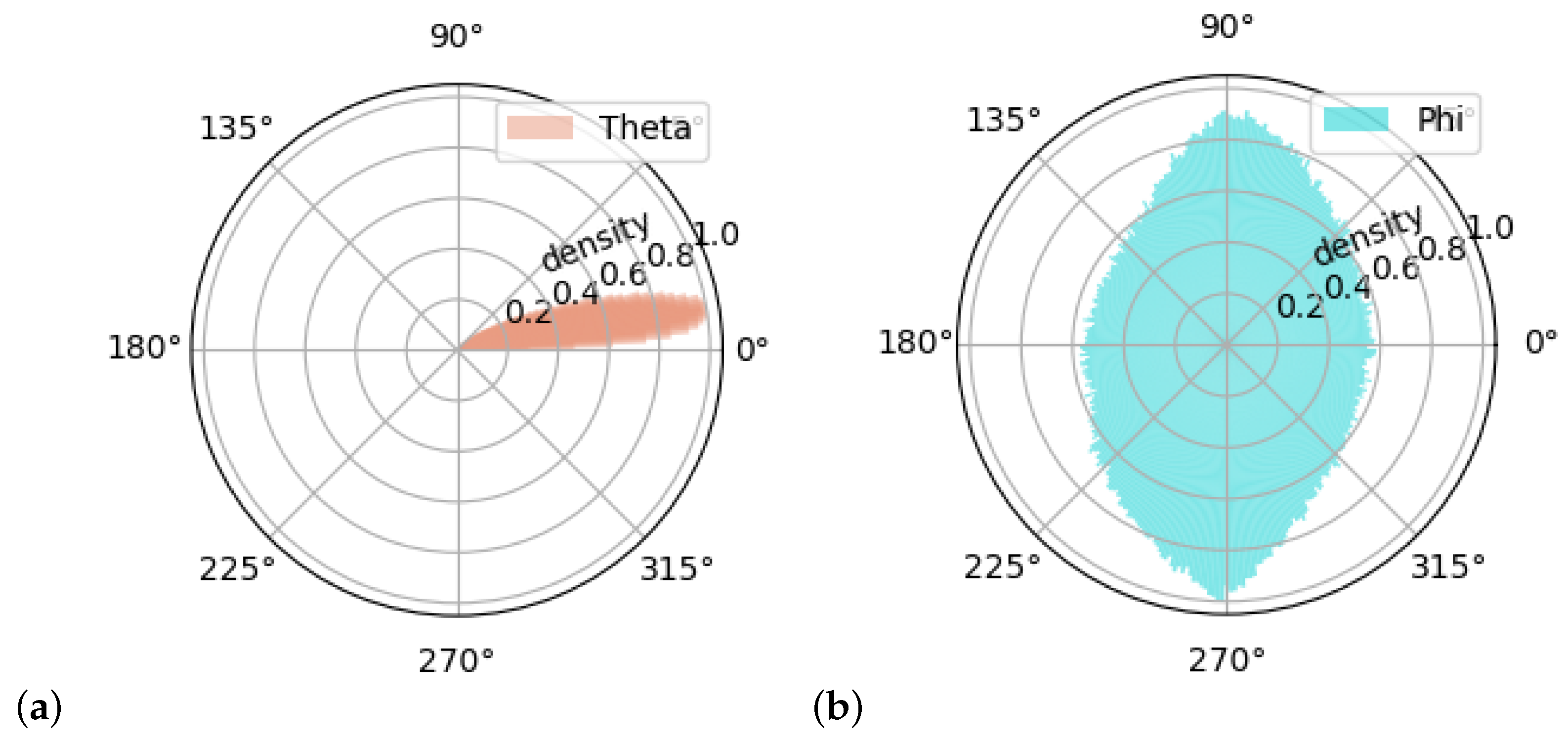
The polar plots of the calculated angle distributions (Figure 11) are useful to understand the steepness of the slopes and the orientation of the surface. The zenith angle $\theta$ tells us information about the steepness of the slopes of the surface under analysis. The azimuth angle $\varphi$ instead indicates if the surface is oriented or if there is a regular distribution of orientation.

As an example, if the surface under analysis has low slopes and is not oriented, the angle $\theta$ will be around $0^{\circ }$ and the $\varphi$ distribution will spread on all angles as reported in Figure 11.

3.2.2. Power Spectral Density

The power spectral density (PSD) [32] function indicates the intensity of different surface frequency components as a function of spatial frequency. It is calculated from the absolute value of the square of the Fourier transform of the height values $z(x,y)$, and the module texture.py implements class Psd, which contains all the methods for PSD evaluation.

The areal Fourier transform is given by Equation (20):

$$F_z(f_x,f_y)=\underset{L_x\to \infty }{lim}\underset{L_y\to \infty }{lim}{\displaystyle \frac{1}{L_x{L}_y}}{\int }_{-L_y/2}^{L_y/2}{\int }_{-L_x/2}^{L_x/2}z(x,y)e^{[-\mathrm{i}2\pi (f_{x}x+f_{y}y)]}\mathrm{d}x\mathrm{d}y$$

(20)

The power spectral density is then calculated as reported in Equation (21):

$$P(f_x,f_y)={\displaystyle \frac{\mathrm{d}}{\mathrm{d}{f}_x}}{\displaystyle \frac{\mathrm{d}}{\mathrm{d}{f}_y}}{F}_z^{\ast }(f_x,f_y)F_z(f_x,f_y)$$

(21)

where $F_z^{\ast }$ is the complex conjugate function of $F_z$ and $f_x,f_y$ are the spatial frequencies of the surface with an area of $L_x\times L_y$.

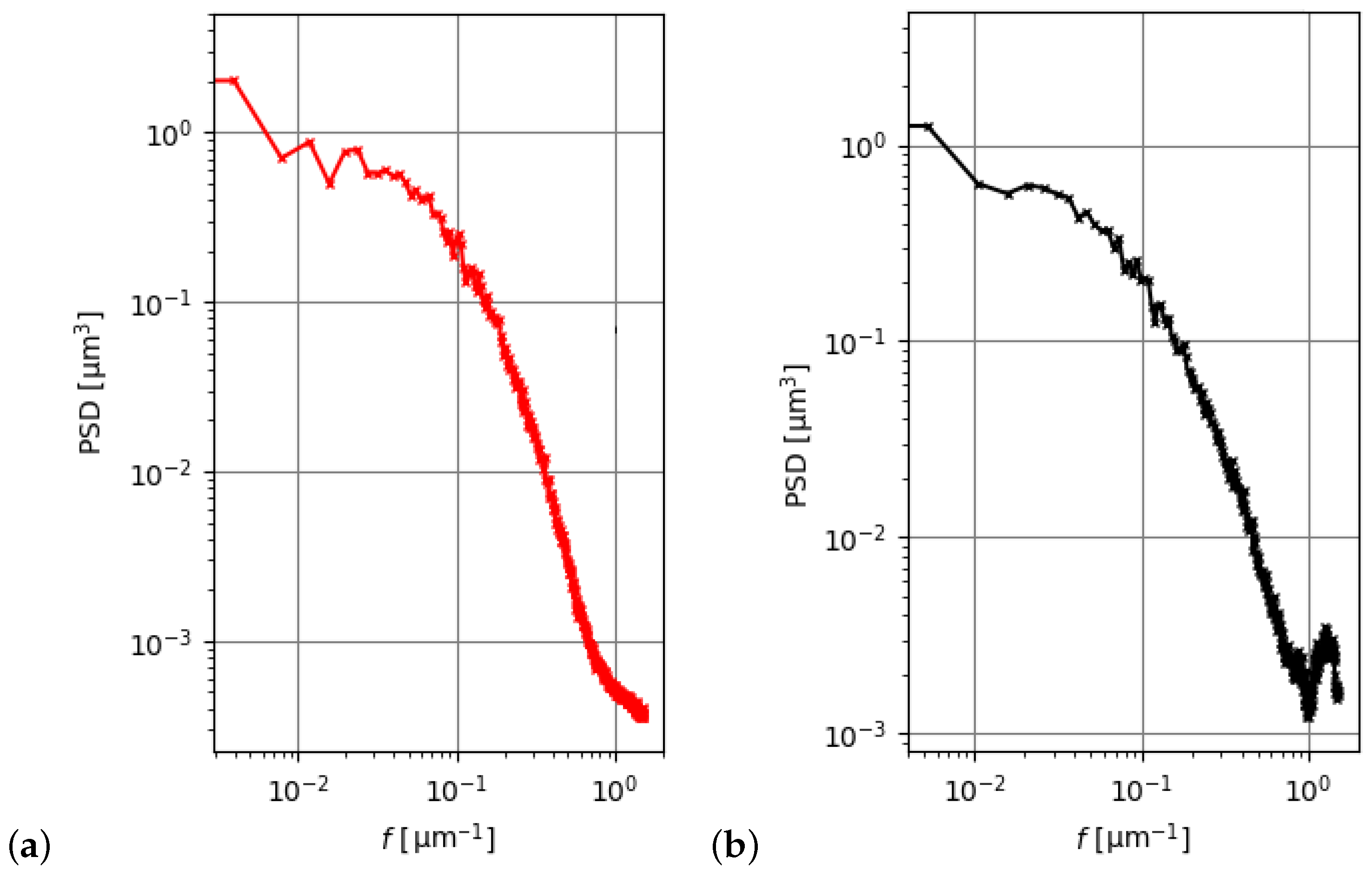
Furthermore, the one-dimensional power spectral densities 1D-PSDs are calculated for each profile in both directions and the average 1D-PSDs $P_x$ and $P_y$ are extracted. The resulting diagrams can be seen in Figure 12, and the two graphs can be used to evaluate the difference in the spectral components between the x and y directions.

This tool is useful to determine the presence of periodical structures in the image that may appear random at first glance; moreover, it gives an indication of the root mean square roughness $R_{\mathrm{q}}$ in the case of profiles and $S_{\mathrm{q}}$ in the case of areal surfaces. These can be obtained by integrating the curve from the L-filter cut-off frequency $f_{\mathrm{L}}$ to the S-filter cut-off $f_{\mathrm{S}}$ as explained in ISO 25178-2:2021 [10]:

$$R_{\mathrm{q},x}^2=2\pi \underset{f_{\mathrm{L}}}{\overset{f_{\mathrm{S}}}{\int }}{P}_x\left(f\right)\mathrm{d}f$$

(22)

Equation (22) reports $R_{\mathrm{q}}$ calculated on the average PSD in the x direction. The same is valid for the y direction, and a double integral on the whole PSD can be used to evaluate the $S_{\mathrm{q}}$ parameter.

3.2.3. Sphere Radius

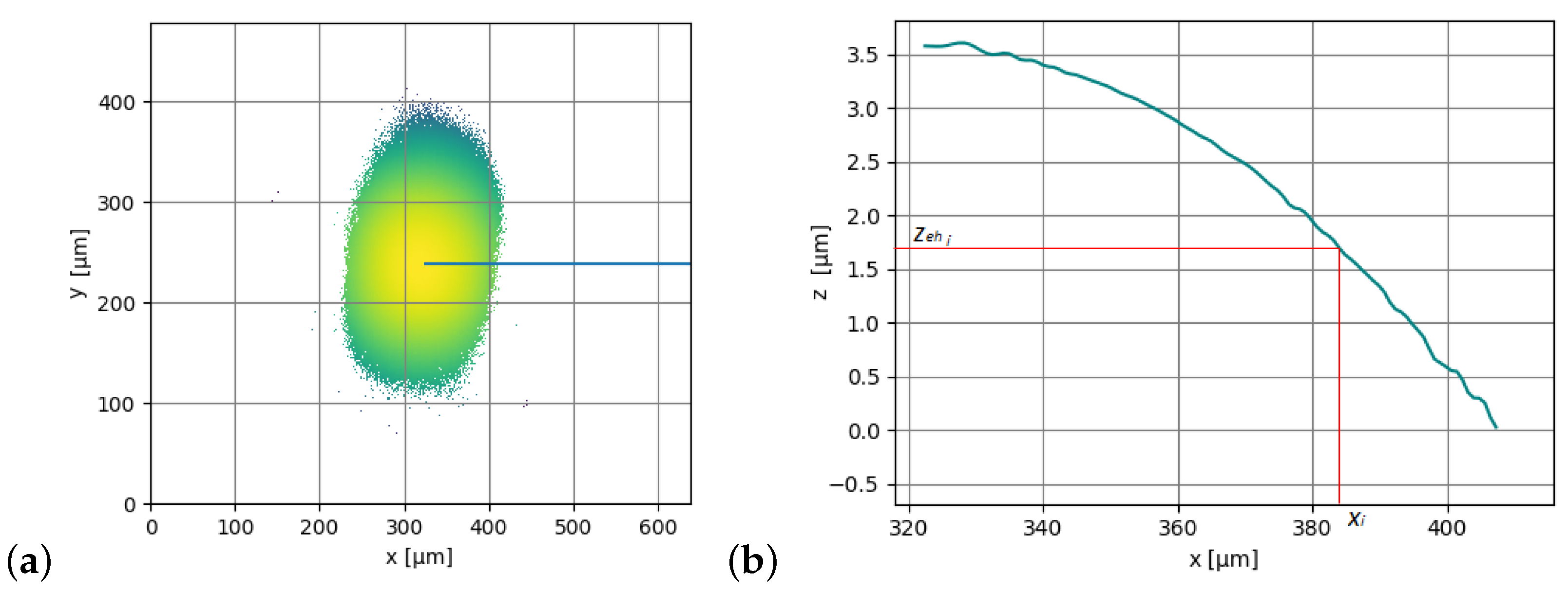
In the module analysis.py, the method SphereRadius calculates the radius of the measured spherical cap radially and at different z values of the extracted cross-section profile.

At first, the method extracts a radial profile from a topography. A radial profile is defined as the points lying on a segment that start from the maximum point of the sphere and end at one of the points located at the perimeter of the topography. The choice of the maximum point is very important and not trivial since noise and distortions can lead to choosing the wrong starting position. The user can specify the method used to find the starting point, and some routines are already implemented, e.g., the center of the least squares sphere can be used as the start point or the local maximum closest to the center of the topography, as shown in Figure 13.

The radius of the sphere for a specific height is then calculated as reported in Equation (23):

$$R_{{\mathrm{radial}}_j}\left(z_{\mathit{eh}}\right)=[R_1,\cdots ,R_n]:R_i={\displaystyle \frac{x_i^2+z_{eh,i}^2}{2z_{\mathit{eh},i}}}$$

(23)

where $x_i^2$ is the x coordinate of the $i_{th}$ point, $z_{(eh,i)}$ is the distance between the maximum value of the profile and the z coordinate of point i, and $R_i$ represent the radius calculated at point i. The mean radius is finally calculated as the average of every radial profile $R_{{\mathrm{radial}}_j}\left(z_{eh}\right)$ for each height, as calculated in Equation (24) and reported in red in Figure 14:

$$R\left(z_{\mathit{eh}}\right)={\displaystyle \frac{1}{M}}\sum _j{R}_{{\mathrm{radial}}_j}\left(z_{\mathit{eh}}\right)$$

(24)

It is important to specify that this algorithm is not the only implemented way to calculate the radius as the spherical fit function explained in Section 3.1.3 also returns the radius of the best-fit sphere.

3.2.4. Maximum Measurable Slope

The maximum measurable slope ${\Phi }_{MS}$ is defined in ISO 25178-600 (2019) [10] as the greatest local slope of a surface feature that can be assessed by the measuring system.

Given a topography of a spherical cap, the method maxMeasSlope of the module analysis.py calculates the maximum measurable slope along the meridians taking into account two different breakpoints for each radial profile. The first breakpoint $R_{ms1}$ is taken at the first non-measured point; the second breakpoint $R_{ms2}$ is taken at the last measured point, as shown in Figure 15a; and the user selects the angular definition of the processing. For every profile, the slope is calculated according to the formulas reported in Equation (25), where R is the nominal radius of the sphere or the radius of the least square fit sphere:

$$\begin{array}{c}{\Phi }_{MS1}=arcsin({\displaystyle \frac{R_{ms1}}{R}})\\ {\Phi }_{MS2}=arcsin({\displaystyle \frac{R_{ms2}}{R}})\end{array}$$

(25)

In Figure 15b, the polar plot of the maximum measurable slope is calculated at the two breakpoints.

3.3. Utilities

3.3.1. Tip Correction

The ISO 21920-2:2021 standard [11] defines different types of profiles:

• Mechanical profiles, describing profiles from contact instruments.
• Electromagnetic profiles, describing profiles from non-contact instruments.

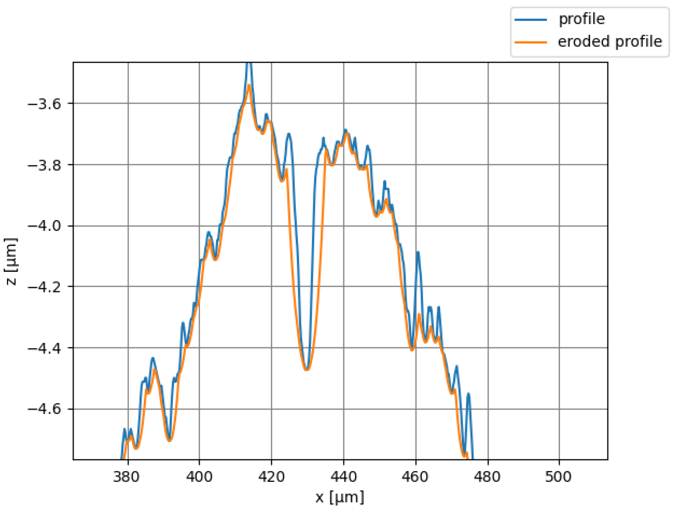
The first type is obtained by applying a tip correction to the skin model of the profile. The processing involves the erosion of the skin model to obtain the locus of points of an ideal circumference of radius r rolled on the bottom of the profile.

At first, the profile is extended with two segments of length r to the left and right. The program then calculates the equation of the semicircle of radius r and superimposes it locally on the profile. The semicircle $c\left(x_{\mathrm{loc}}\right)$ (Equation (26)) is calculated over n values between the two extremes of the circle, where $\alpha =x_i$ and $\beta =p\left(x_i\right)-r$ are the circumference center coordinates expressed as reported in Equation (27):

$$c\left(x_{\mathrm{loc}}\right)=\sqrt{-({\alpha }^2-r^2)+2\alpha x_{\mathrm{loc}}-x_{\mathrm{loc}}^2}+\beta$$

(26)

$${(x-\alpha )}^2+{(y-\beta )}^2=r^2$$

(27)

Since the radius of the circle is an order of magnitude larger than the profile sampling, it is necessary to interpolate the profile in $x_{\mathrm{loc}}$ to compare the two functions locally. At this point, the program tries to find the smallest value of $\beta$ that brings the semicircle completely below the profile. To minimize the number of iterations, the bisection method was implemented. Once the correct position of the semicircle is found, the program proceeds with the next point of the profile until the filtered profile is obtained. The result is shown in Figure 16 and it shows how the algorithm sharpens the peaks and broadens the valleys of the profile.

In addition to this method, the naïve approach explained in [22] was implemented in the package.

3.3.2. Stitching

The problem of consistently aligning two surfaces or point clouds can be formulated as an optimization problem in which the rigid translation that best overimposes the points of the first surface with those of the second must be found. The implemented program provides two different methods in the module stitcher.py:

• Correlation stitching.
• FGR stitching.

Methods that consider surface deformation are not yet implemented in the package.

Cross-Correlation Stitching

The method SurfaceStitcher.stitchCorrelation finds the best translation (in pixel units) in the $x,y,z$ directions by cross-correlating the two stitching regions of the surfaces. The solution explained in [26] is here modified to improve the probability of detecting the correct translation.

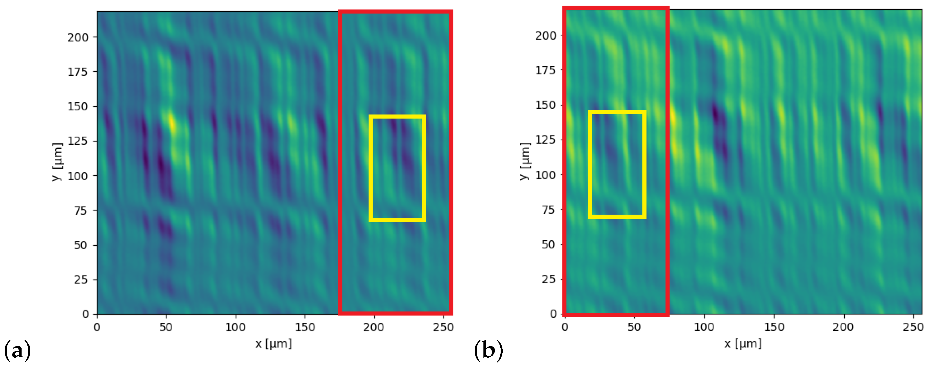
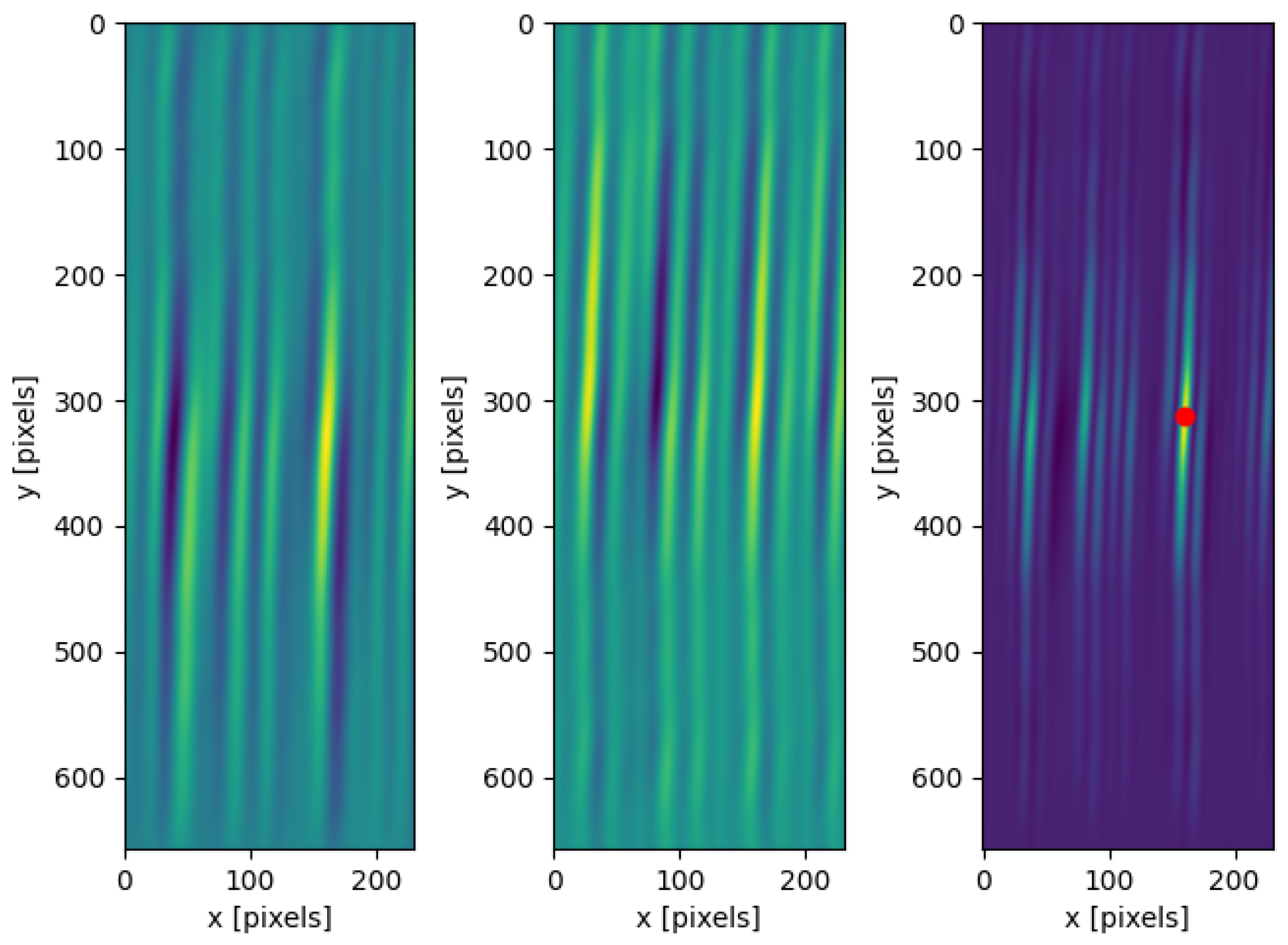
Let the input topographies be those expressed in Equation (28) and shown in Figure 17:

$$z_l(x,y)z_r(x,y)$$

(28)

The user must provide the theoretical stitching percentage of the images $\alpha$ and the sampling percentage $\beta$. The program then extracts the regions of interest from the input surfaces. The first parameter is used to isolate the leftmost part of the right image and the rightmost part of the left one. The second parameter is the percentage of the two isolated zones considered for the cross-correlation.

Once the zones are extracted, two cross-correlation matrices are computed between the opposite zones. Since the images to be stitched often exhibit periodical values, the cross-correlation can show multiple local maxima of similar intensity, all valid candidates to be the best translation result. To pinpoint the correct maxima, one of the two cross-correlations is rotated around the center point and multiplied by the second one. In this way, only the points with a high correlation in both zones are considered valid candidates for the final translation.

Figure 18 shows how the multiplied cross-correlation is able to pinpoint the translation that has a maximum in both left and right topographies. Once the correlation is finished, the best final translation can be calculated by finding the index of the maximum value in the multiplied cross-correlation matrix and subtracting the central value index of the topography.

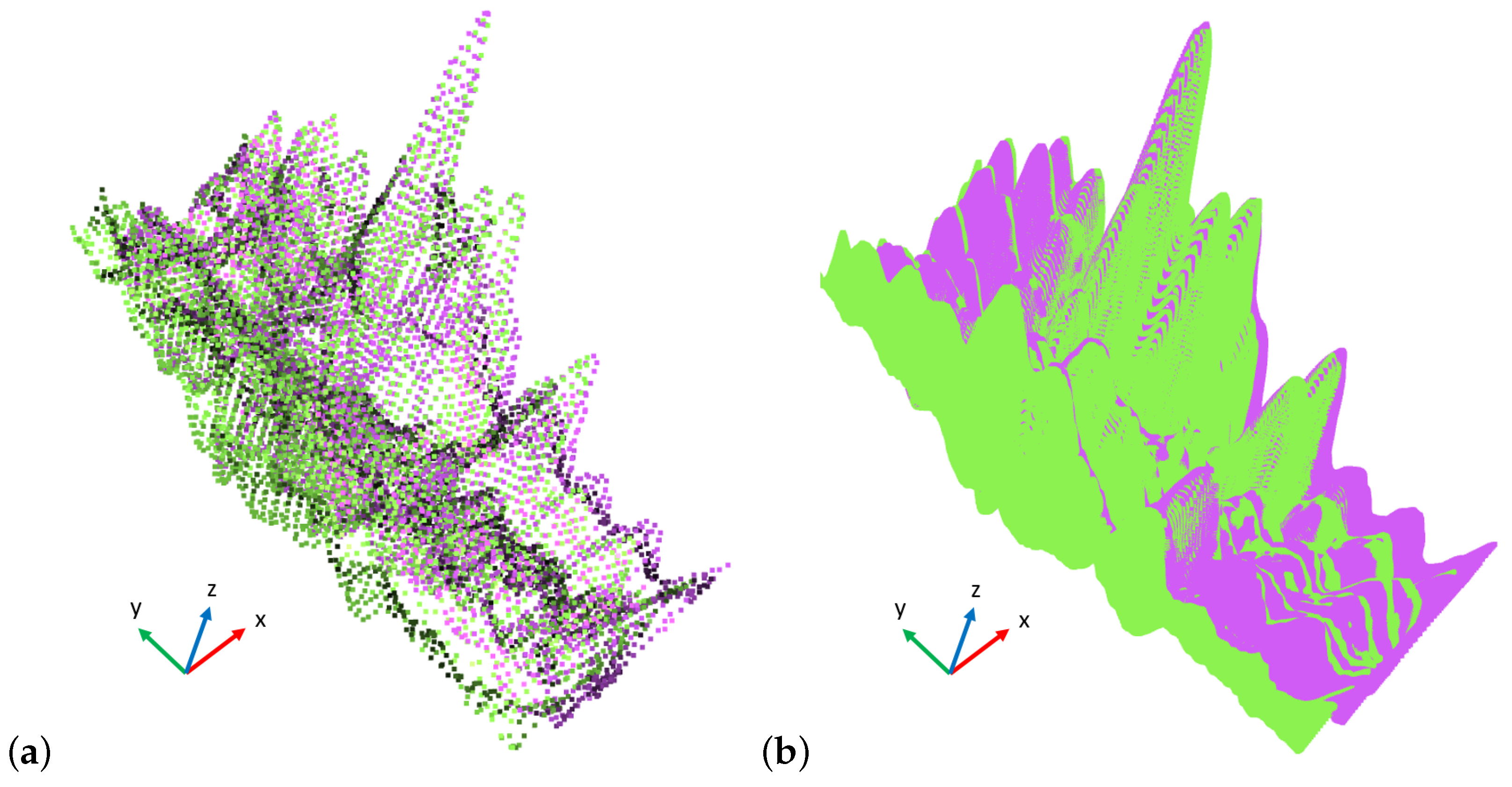
Fast Global Registration (FGR) Stitching

The method SurfaceStitcher.stitchFGR provides an implementation of the open3d library [33] FGR algorithm [27] adapted to surface processing.

First, the program isolates the zones of the images as described in the section cross-correlation stitching, so the obtained topographies are converted from x, y, z matrices to point clouds. The dimensions of the point clouds are normalized with the same normalization values such that all the dimensions are between 0 and 1 without modifying the proportions between the left zone and the right zone. Given a desired voxel size, the program downsamples the point clouds to reduce the number of voxels to be processed, speeding up the calculations. After calculating the normal vectors of all points, the PFH (point feature histogram) features are calculated using the FPFH (fast PFH) algorithm [34]. Based on these features, the nearest neighbor is found for each point among the points on the other point cloud. To improve the quality of the matches, two tests are carried out, as explained in [27]. After the FGR algorithm is executed, a 4 × 4 transformation matrix is returned. This transformation can also be used as a good starting point for the ICP (Iterative Closest Point) registration algorithm that further refines the matrix values. Figure 19 shows the two stitching results applied on the same sample as the cross-correlation case.

3.4. Experimental Setup and Samples

The implemented package was used in the framework of the interlaboratory comparisons between national metrology institutes related to the TracOptic project to best suit the samples analyzed, which are

• SiMetricS Resolution Gratings RS-M 3 [35], used for the calibration of optical profilometers and AFM at smaller scales;
• Lambda Research Optics $\lambda /10$ mirror [36], used for noise quantification;
• Saphierwerk AG ruby Spheres [37], used for the determination of the maximum measurable slope of each objective [37];
• Bruker Alicona µContour standard cylinders [38];
• SiMetricS Flatness Standard FtS [35], used for noise quantification and power spectral density (PSD) comparison.

The measurements on these samples were carried out with the optical profilometer Sensofar PL$\mu$ 2300, metrologically characterized in INRiM using calibrated interferometers directly traceable to the national meter standard.

4. Results and Discussion

In order to verify the methods implemented in SurfILE, we compare our results with the ones obtained by the surface metrology software Digital Surf MountainsMap^® 9.3 and Gwyddion 2.61 on different kinds of samples.

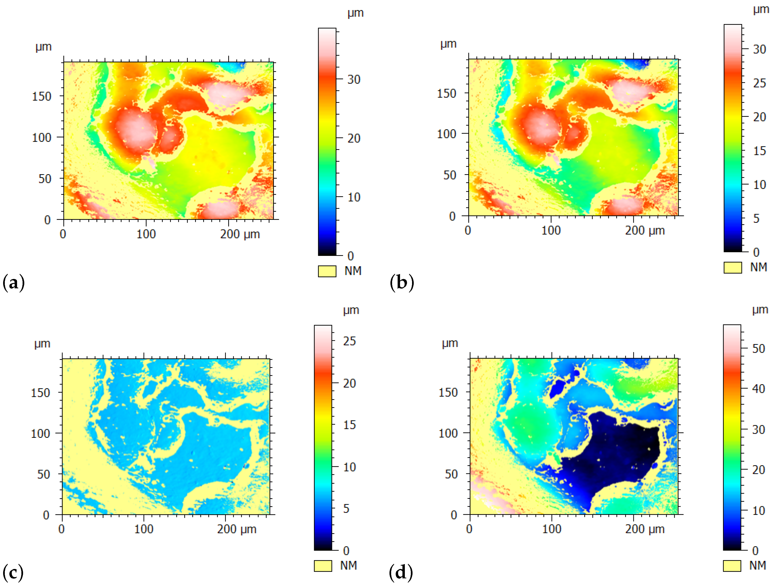
For form removal operations, the comparison method employed involves fitting the same dataset using both SurfILE and MountainMap and subsequently evaluating the standard deviation of the differences between the surfaces obtained after the form removal process. This approach allows for a quantitative assessment of the performance of each software in accurately removing the form from the surface data. Figure 20 illustrates the procedure followed for this comparison, detailing the steps taken and presenting the results obtained for various types of form removal operations. The results of this comparison are summarized in

Table 1. Comparison of form removal operations between SurfILE and MountainsMap on different samples.

Measurands	Sample	RMS Parameter [$\mathsf{\mu }$m]	Software Difference [%]
Least square form removal of a plane	Plastic roughness sample	0.29	0.3
Least square form removal of a 2nd-order polynomial surface	Plastic roughness sample	0.30	0.8
Least square form removal of a line	Plastic roughness sample	0.35	0.6
Least square form removal of a 2nd-order polynomial profile	Plastic roughness sample	0.35	0.3
Least square spherical fit	Saphierwerk AG Ruby sphere $r=350\mathsf{\mu }$m	0.06	0.7

, which reports the deviation of the results as the RSM parameter Rq in the case of profiles and Sq in the case of surfaces for each method, providing a clear overview of the discrepancies observed. The RSM parameters are a good indicator of the flatness of the result since the peaks and valleys are taken into consideration quadratically.

In the case of polynomial fits, the analysis extended beyond the calculation of the root mean square (RSM) parameters, and a comparison of the polynomial coefficients was also conducted. However, due to the different implementations of coefficient matrices in the two software packages, the comparison was not trivial. Specifically, Gwyddion uses a full coefficient matrix implementation while MountainsMap employs only the upper-left triangle of the matrix. This discrepancy complicates direct comparisons of the coefficients as the two methods do not provide equivalent outputs for the same input data.

It is also important to point out that neither MountainsMap nor Gwyddion supports the removal of a five degrees of freedom cylinder, which precluded a direct comparison of this specific method. During the TracOptic project, the $\mu$contour standard sample [38] was distributed among the project partners to aid in measuring various cylinders with different radii and concavities. A significant number of measurements were taken at various orientations to evaluate the radius and form deviations of the samples. This diversity of experimental conditions created a thorough testing environment for the fitting routine used in the analysis. The results consistently indicated that the fitting routine performed as anticipated, irrespective of the orientation of the cylinders being examined. This consistent performance highlights the reliability of the fitting method across a variety of practical situations, further confirming its usefulness in real-world surface analysis applications.

For the slope distribution verification, the results were compared with both MountainsMap^® 9.3 and Gwyddion, and the distributions obtained are very similar for all three software, as can be seen in Figure 21. The verification was carried out using a non-adaptive histogram explained in Section 3.2.1, and for this reason, the Gwyddion result is slightly different since the open-source program implements the adaptive approach.

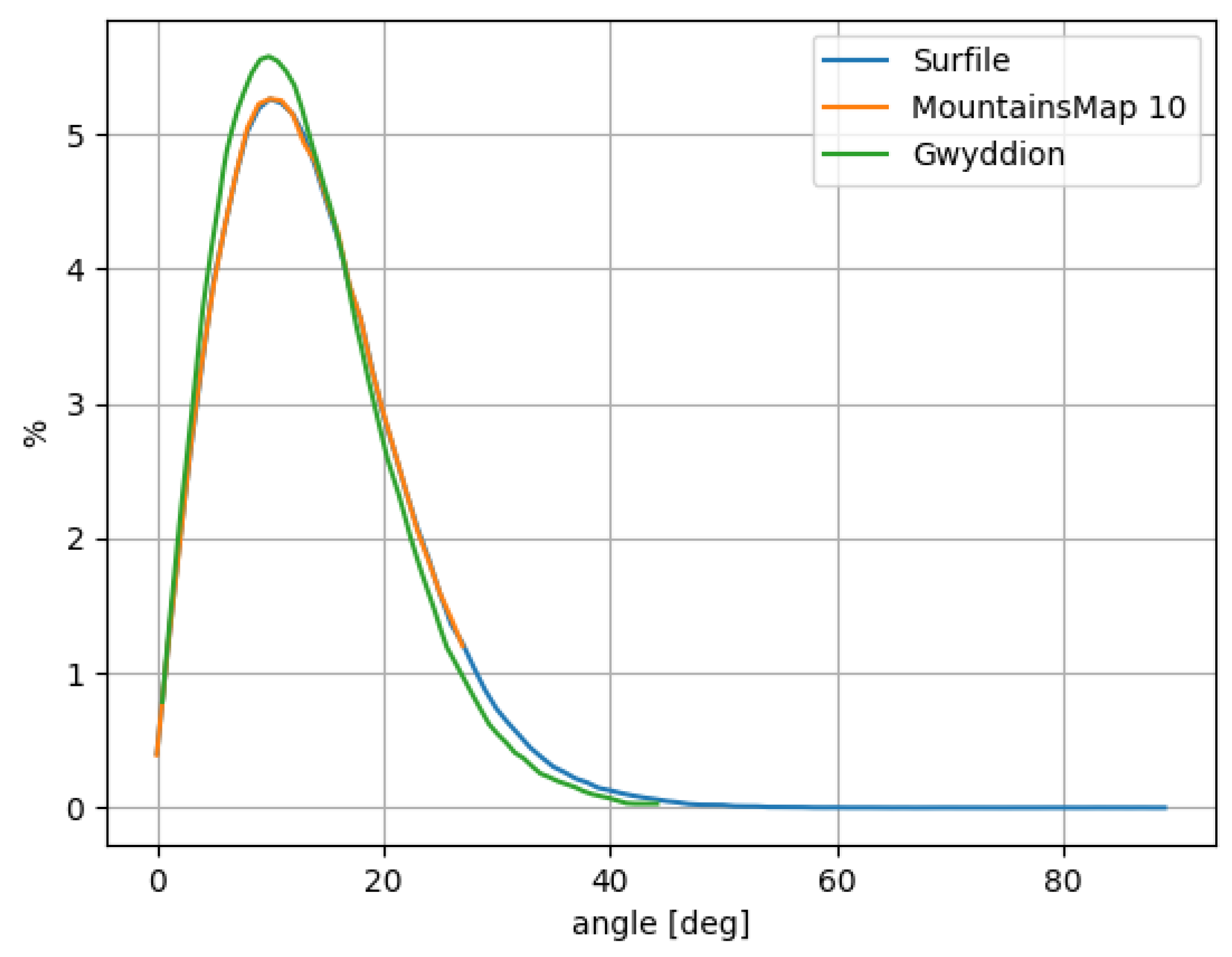
The power spectral density routine was compared both with Gwyddion and MountainsMap. For the latter, it was necessary to adapt the result spectra to standard units since the commercial software provides the result in $\mathsf{\mu }{\mathrm{m}}^{-1}$ on the x-axis and $\mathsf{\mu }{\mathrm{m}}^2$ on the y-axis while both SurfILE and Gwyddion provide the spectra in $\mathsf{\mu }{\mathrm{m}}^{-1}$ on the x-axis and $\mathsf{\mu }{\mathrm{m}}^3$ on the y-axis. To make the results compatible, the MountainsMap y-axis values were multiplied by the length of the topography. This discrepancy between the software was brought to the attention of the MountainsMap team to confirm our correction of the data. This also led to a correction in the latest release of the commercial software (Figure 22).

The maximum measurable slope was determined for two different objectives using a set of 16 × 5 spherical cap topographies, which were created by combining four ruby spheres of varying diameters with different orientations and objectives. Specifically, for each sphere, two perpendicular orientations were analyzed for each objective, resulting in a total of 16 distinct measurement conditions. Each measurement was repeated five times for statistical purposes, leading to a total of 80 images. As shown in Figure 23, the analysis indicated that variations in the sample being examined and its orientation did not influence the maximum measurable slope of the objective used for the measurements. This outcome is consistent with our expectations regarding the software’s capabilities, confirming its reliability across various experimental configurations. However, it is important to note that for the 50× objective, the 1000 $\mathsf{\mu }\mathrm{m}$ ruby sphere could not be utilized in the maximum measurable slope analysis since the objective’s field of view was insufficient to capture the end curvature of the measured cap, thereby precluding a complete radial assessment of the slope in this instance.

The radius calculation was also used to evaluate the dimensions of the four ruby spheres, and the results obtained are compatible with the least square spherical fit radius calculation.

To ensure that the routines meet the demands of practical applications, the processing speeds for the majority of the implemented methods are satisfactory, generally falling within the range of a few seconds or tenths of a second per image. This level of efficiency is crucial for users who require a rapid analysis of large datasets. The ability to process images quickly without compromising the accuracy of the results is a significant advantage, particularly in industrial settings where time constraints are often critical factors.

It is important to note that the majority of the methods implemented were used in the framework of the TracOptic project [8] and that the results obtained from the processing during the interlaboratory comparisons were compared with other NMI results.

5. Conclusions

We presented SurfILE, a Python package for the processing of digital topographies in the field of nano- and micro-dimensional metrology. The implemented methods are resilient and can be easily customized by even inexperienced programmers, laying a solid foundation for future program development and open-source contributions. The results obtained were compared with software already present and used by the scientific community, and good agreement was found between the results.

The variety of samples used during international comparisons has greatly expanded the software’s ability to adapt to multiple processing possibilities. The inherent modularity of Python packages and the flexibility of object-oriented programming allow for the generalization of methods for removing sample shapes, filters, and cutters, resulting in efficient code reuse. Code documentation is complete and easily readable in html format, and the methods can be easily used in a Python script by consulting the reference provided.

Key innovations include a double correlation stitching method and a five degrees of freedom cylinder fitting approach, both of which are not available in existing commercial software. Additionally, the package offers adaptive and non-adaptive slope distribution analysis, as well as a fast global registration stitching method tailored for surface metrology, which incorporates an Iterative Closest Point (ICP) optimization algorithm, an enhancement that has only recently been integrated into commercial solutions. Furthermore, the package supports polynomial fitting on periodic structures and introduces a radial maximum measurable slope with a double breakpoint for objective characterization.

While numerous programs with graphical user interfaces (GUIs) are already distributed and widely utilized in the field of surface analysis, our package offers a distinct advantage by providing greater flexibility in the analysis of large batches of images. Specifically, it is designed to handle hundreds of images that may share similar shapes yet possess varying quantitative characteristics. This capability is particularly beneficial for researchers and industry professionals who often encounter datasets where images exhibit common geometric features but differ in critical parameters such as texture, roughness, or other surface metrics. Furthermore, the flexibility allows users to customize their analysis methods according to the specific requirements of their datasets, facilitating a more tailored and effective examination of surface properties. This adaptability not only improves the accuracy of the results but also empowers users to derive deeper insights from their data.

The software allows for method real-time analysis and batch result reporting, providing a simple decorator designed to streamline the process of data analysis and enhance the readability of the results. This functionality not only facilitates the execution of various analytical methods on a batch of images but also automates the generation of customizable reports in CSV format. The ability to produce structured reports is particularly beneficial for researchers and professionals operating within the framework of digitalization and Industry 4.0. Furthermore, the standardized format of the CSV files ensures compatibility with a wide range of data analysis platforms, making it easier for users to integrate the results into their existing workflows. Moreover, the package processing methods were validated and evaluated for speed, revealing that most methods operate efficiently, typically completing analyses within seconds or fractions of a second per image.

Collectively, all these features present in the SurfILE package provide researchers and industry professionals a robust tool for enhanced data interpretation in the field of surface analysis.

Future developments of the program will include (i) the integration of filtration algorithms, such as surface filters and more advanced morphological filters, and (ii) the refinement of the stitching algorithms.