Article

Novel Method of Fitting a Nonlinear Function to Data of Measurement Based on Linearization by Change Variables, Examples and Uncertainty

by
Zygmunt L. Warsza
1,*,
Jacek Puchalski
2 and
Tomasz Więcek
3
1
Industrial Research Institute for Automation and Measurements, Polish Metrological Society PTM, Warsza Szmaragdowych Żuków 32, 05-540 Zalesie Górne, Poland
2
Central Office of Measures GUM, Elektoralna 2, 00-139 Warsaw, Poland
3
Department of Applied Optics, University of Technology Rzeszow, 35-959 Rzeszów, Poland
*
Author to whom correspondence should be addressed.
Metrology 2024, 4(4), 718-735; https://doi.org/10.3390/metrology4040042
Submission received: 14 August 2024 / Revised: 12 November 2024 / Accepted: 15 November 2024 / Published: 3 December 2024
(This article belongs to the Collection Measurement Uncertainty)

Abstract

:
This paper presents a novel method for determining parameters and uncertainty bands of nonlinear functions fitted to data obtained from measurements. In this procedure, one or two new variables are implemented to linearize this function for using the linear regression method. The best parameters of the straight-line in new variables are adjusted to the transformed coordinates of tested points according to the weighted total mean square criterion WTLS, or WTLS-C of data points are also correlated. Uncertainties of measured points are found according to the rules of the GUM Guide. The parameters and the uncertainty band of the nonlinear function result from the parameters of this straight line and of its uncertainty band. A few examples determining the parameters and uncertainty bands of different types of nonlinear functions are presented. There are also examples of measurements using the presented method and conclusions.

1. Introduction

The nominal characteristics of many sensors, transducers, measuring instruments and systems, as well dependencies on the parameters of studied phenomena, material properties, characteristics of devices and their components can be described by nonlinear functions. Measured characteristics and their uncertainties are also compared with these nominal data to ascertain whether they meet specific requirements. Then, the parameters of nonlinear functions are matched to data of measurement points and their uncertainties, according to the international guide GUM [1] and its Supplements.
The literature for fitting nonlinear functions to data of measurement is not so rich as for linear functions with the application of linear regression. The oldest one is the Gauss–Newton method from 1809 [2,3,4,5]. Later developed were the quasi-Newtonian methods by Davidson, Fletcher and Powell, the Levenberg–Marquardt method in 1949-63 [2,3,6], the BFGS methods and other numerical methods which include the gradient method of solving nonlinear equations [7,8,9,10,11,12,13,14,15,16]. The artificial neural net methods (ANN) are now also used for the fitting of nonlinear functions. An example of the ANN method is described by Li M., and Verma B. in [17], and the ANN method based on the optimized extreme learning machine is also described by Li. M. with Li L.D. and others in 2020 [18].
Currently, when fitting the nonlinear functions to data of measurements, only the numerical and ANN methods are useful. Their algorithms are quite sophisticated. However, they are not universal, are too complicated for applications in routine measurements and do not consider all uncertainties of measured points according to actual recommendations in the GUM [1,19] and all possible correlations, as is needed in metrology. For such applications, we have developed a novel analytical method based on linearizing the measurement function by changing variables. The theory of this method and optimization of function parameters according to the minimum WTLS criterium is presented. Then, some examples of the application of new variables for linearizing three basic types of nonlinear function forms and fitting them are provided. The application of this method in a few measurement experiments is also demonstrated.

2. Main Idea of Proposed Method

In this the novel analytical method of fitting—nonlinear functions to data of measurement [20,21,22], the replacement of primary measured variables by the new variables is used in such a way that the linear regression of the straight line can be applied. If the tested points are not too far from the desired function fitted to them, and if values of the uncertainties of measurement data are not too large, e.g., below 5%, then this method can be successfully used. These limitations are of the same order as in the GUM for estimating uncertainties. From the mathematical point of view, the proposed method involves the transformation of the equation described by the nonlinear functions into a description by linear functions of the new Cartesian coordinates [20,21,22]. In this way, the variables x, y, as coordinates of the measured points, are replaced by new variables ξ ,   ψ to obtain a straight line in their Cartesian system. These new variables are differentiated functions of y and x. It is also assumed that they can be parameterized.
We will generally discuss, now, the sequence of steps for the proposed method of variable replacement. At the beginning, a form of equations relating to the real coordinates x, y of the nonlinear function under consideration and the new coordinates ψ, ξ are selected to obtain a linear relationship for that function and the relationship between their uncertainties.
New coordinates ( ξ i, Ψ i ) of measured points (xi, y i ) are found and their standard uncertainties are determined according to the principles of the GUM [1]: u i = ( u A i   ) 2 + ( u B i ) 2   . The uncertainties u A . result from the statistics of the dispersion of the measurements of coordinates of each point. The estimated uncertainty u B is for unknown systematic errors of the measuring instruments. If correlations of measurement data are present, their influence must also be considered. The parameters of the straight line fitted to these points according to the appropriate least squares criterion and the contours of the boundaries of the bands (corridors) of the standard and expanded uncertainties of this straight line are found. Then, using the inverse functions of both types of coordinates, one returns to the considered nonlinear function and determines its parameters and its uncertainty band in primary x, y coordinates to ascertain probability.
In measurement practice, there are many different types of measurement experiments. Measurements can be made only for one of the tested points’ coordinates, e.g., y, and the values of the other one, i.e., x, are precisely known. Both variables x and y can also be measured. The results xi, y i . can be uncorrelated or may have mutual correlation. Furthermore, the measured results of one or both coordinates of different tested points also can be autocorrelated.
The nonlinear functions relating to the variables x, y can appear in many different forms. For the proposed method we considered the following three types of nonlinear functions:
  • The simplest form with the determined dependent variable y, i.e., y = f (x).
  • On each side of the equal sign are nonlinear functions of only y or x, f y ( y ) = f x ( x ) .
  • The implicit form of the nonlinear function H(x, y) = 0.
We calculated numerical examples of the different possible replacements of variables, determined their function parameters and uncertainties, and the limits of the uncertainty bands with specified probability. A few examples are discussed below.
For the nonlinear function y = f(x) the straight-line equation in the new Cartesian coordinates ψ , ξ has the form
ψ ( y ) = θ 1 ξ ( x , β ) + θ 0  
The parameters of linear Equation (1) can be adjusted by the linear regression method to the measurement data of tested points after changing their coordinates x, y to ψ , ξ and by using the WTLS least squares method. From the minimum of this criterium, the parameters θ 1 , θ 0 ,   β are determined, and from them the parameters and uncertainty band of the nonlinear function y = f(x) fitted to measurement data of tested points is calculated.
The function, which includes the covariance matrix, is also transformed and is expressed by uncertainties in the new coordinates. Assuming the propagation laws of errors and of uncertainties, which means the use of only the first derivatives of transforming functions, an approximately identical criterion value of the objection function for regression and alignment to a straight line in the new coordinates is obtained as the adjustment of a nonlinear curve in the original coordinates.
The uncertainties in the new Cartesian coordinates result indirectly from this linear approximation. For Gaussian density distributions the following relations are applied: u ( ψ ) | ψ ( y , β ) | u ( y ) , and u ( ξ ) | ξ ( x , β ) | u ( x ) .
Relation between WTLS-C criterium in x, y coordinates and in new Cartesian coordinates ψ , ξ in general case takes the form
ϕ x y ( Δ X , Δ Y ) = [ Δ X , Δ Y ] L L 1 [ U X U X Y U X Y T U Y ] 1 L 1 L [ Δ X Δ Y ] ϕ ψ ξ ( Δ ξ ,   Δ Ψ , β ) = [ Δ ξ   , Δ Ψ ] [ U ξ   U ξ   Ψ U ξ   Ψ T U Ψ ] 1 [ Δ ξ   Δ Ψ ]  
where
U X = [   u x 1 2     ρ x 1 n u x 1 u x n ρ x 1 n u x n u x 1   u x n   2 ]   , U Y = [ u y 1 2     ρ y 1 n u y 1 u y n ρ y 1 n u y n u y 1   u y n   2 ]   , U X Y = [   ρ x 1 y 1 u x 1 u y 1 ρ x n y 1 u x n u y 1             ρ x 1 y n u x 1 u y n ρ x n y n u x n u y n ]   ,   L = [ ξ ( x 1 , β ) 0 0 ξ ( x n , β ) 0 0 0                             0 0                           0 0 0 ψ ( y 1 , β ) 0 0 0 ψ ( y n , β ) ]
Data of measurement points and covariance matrices in the new coordinates are given by vectors ξ , Ψ , and by matrixes U ξ , U Ψ ,   U ξ Ψ . Only the β is an unknown parameter. Its constant value should be chosen to minimize the criterion function ϕ ψ ξ . Its uncertainty is negligibly small, i.e., u ( β ) 0 . When transforming vectors X, X p and Y , Y p , respectively, into vectors ξ ,   ξ p and Ψ , Ψ p , with (2) and (4) in order to fit a nonlinear function, a system of two vector equations is obtained, i.e., the description of minimization of the new criterion function ϕ ξ ψ , and the equation of a straight line, are both given below:
{ ϕ ψ ξ ( Δ ξ ,   Δ Ψ , β ) m i n Ψ p = θ 1 ξ p + θ 0  
where θ 0 = θ 0 [ 1 , , 1 ] T .
Searching for a minimum means that
ξ p ϕ ξ ψ = ϕ ψ ξ Δ ξ = 0   ,       ϕ ξ ψ θ 1 = 0         and       ϕ ξ ψ θ 0 = 0
The first condition is solvable analytically and leads to obtaining a local minimum for the inverse effective covariance matrix, as follows:
U Y e f f 1 = U 22 ( U 12 T + θ 1 U 22 )   V 1 ( U 12 + θ 1 U 22 )
and the covariance matrix in new coordinates
Q = [ U ξ   U ξ   Ψ U ξ   Ψ T U Ψ ]   and   Q 1 = [ U 11   U 12 U 12 T U 22 ]
V = U 11 + θ 1 ( U 12 T + U 12 ) + θ 1 2 U 22
If we are dealing with measurement points of not correlated coordinates, then the covariance matrix is diagonal, as follows:
[ U Y e f f ] i i = θ 1 2 u 2 ( x i ) + u 2 ( y i ) .
In general cases the criterial function is a quasi-quadratic:
ϕ ξ ψ ( θ 1 ) = θ 1 2 ( S ξ ξ S   ξ 2 S ) + 2 ( S ξ S ψ S S ξ ψ ) θ 1 + S ψ ψ S   ψ 2 S
where   S ξ ξ = ξ T U Y e f f 1 ξ ,   S ψ = Ψ T U Y e f f 1 1 = 1 T U Y e f f 1 Ψ ,   S ψ ψ = Ψ T U Y e f f 1   ξ , S ξ ψ = ξ T U Y e f f 1 Ψ = Ψ T U Y e f f 1 ξ and θ 0 = (   S ψ θ 1   S ξ ) / S .
As we see from (10), the dependence of   ϕ ξ ψ ( θ 1 ) is always quasi-quadratic for any given β . From equation (10) we always obtain the same type of two dimensional characteristics of criterial function ϕ ξ ψ ( θ 1 , β ) or ϕ ξ ψ ( θ 0 , β )—see Figure 1.
To determine the boundary of the uncertainty band, the variance for a straight line is determined after the numerical determination of matrix of sensitivity coefficients C and the covariance matrix U θ 1 θ 0 = C Q C T composed of parameters u ( θ 1 ) ,     u ( θ 0 ) ,     ρ θ 1 θ 0   with the equation
u y 2 = u 2 ( θ 1 ) ξ 2 ( x , β ) + 2 ρ θ 1 θ 0 ξ ( x , β ) u ( θ 1 ) u ( θ 0 ) + u 2 ( θ 0 ) ( ψ ( y )   ) 2  

3. Examples of Nonlinear Functions Fitted by Change Variables for Linearization

The numerically determined expanded uncertainty characteristics as well as the parameters of the adjusted curves were compared with the nominal curves. All results were demonstrated in tables and graphs. Only parabola describing measured data without correlations can be checked by the analytical method. The effectiveness of the applied novel method has also been confirmed.

3.1. Transformations of Single Coordinate x (Type I)

We will consider an example of fitting a characteristic described by a second-degree function as a branch of a parabola [20,21,22] with the equation
y = A x 2 + B x + C
or in canonical form
y = A ( x + B 2 A ) 2 + C B 2 4 A
By changing the variables accordingly, this equation can be transformed into a linear equation and adjusted to the new coordinates of the test points. Below, we considered method I of fitting a parabolic curve from two methods described in [21].

Parabola Fitting—Method I

Method I is to convert the x coordinate into a new Cartesian coordinate ξ ( x , β ) = ( x + β ) 2   with use substitutions θ 1 = A , β =   B 2 A   , and θ 0 = C B 2   4 A . The ordinate does not change, i.e., ψ = y . Equation (13) will be transformed into the form
y = θ 1 ξ + θ 0
Measurement errors are determined by approximations using the equation:
Δ ξ i ξ x i Δ x i = 2 ( x i + β ) Δ x i
The uncertainty of the new coordinate ξ is determined by the law of uncertainty propagation. For small values, only words with the first derivative are considered, as shown below:
u ( ξ i ) | ξ x i |   u ( x i ) = 2 | x i + β |   u ( x i ) ,   i = 1 ,   ,   n ,
As an example, we will consider simulated tests of the actual processing characteristics of a voltage converter with a rated parabolic characteristic generally described using Formulas (12) and (13). To determine the value xi of its input voltage x, the yi values of the output voltage y were measured. Measurements of both voltages were made with a meter of standard relative uncertainty δ = 1%. Table 1 shows the values of the two measurement point coordinates and the simulated deviations Δy from the nominal characteristics, using the equation: y = 2 x 2 + 3 x + 4 .
Using an EXCEL workbook (Fit, parabola I.xlsx ver.1.01), based on measurement data from ten points, the values of the function were determined ϕ ξ ψ ( θ 1 ) . The formulas for the effective inverse matrix to the covariance matrix and auxiliary parameters the authors used in [20,21,22]. Minimization was made by means of a parameter by β monitoring the determined characteristics ϕ ξ ψ ( θ 1 ) containing a local minimum. For parameter matching β = β m i n a global minimum is obtained. This is illustrated in Figure 2a.
For the same data of sampling points, the characteristics of the ϕ ξ ψ ( θ 0 ) use the unambiguous relationship between the value of the free term and the value of the direction coefficient at the point of the global minimum of the function ϕ ξ ψ —see Figure 2b.
For the minimum of the criterion function, the following formulas for the parameters of the parabola are obtained, using
A = θ 1 m i n ,   B = 2 A β m i n = 2 β m i n θ 1 m i n ,     C = θ 0 m i n +   β m i n 2 θ 1 m i n
Matched second-stage function with uncertainty band ± U y ( x ) describes the equation:
y = θ 1 m i n   ( x + β m i n ) 2 + θ 0 m i n ± U y ( x )
where the expanded uncertainty   U y   with Formulas (7) and (8).
From coordinate values of the global minimum point in Figure 2a,b, the following parameters of the fitted second-degree parabola were obtained: A = 2.044 , B = 2.70 , C = 5.14 . Together with the uncertainty band, it is shown in Figure 3a.
After assuming the same autocorrelation coefficients +0.2 for matrix elements UX, UY and negative coefficients −0.2 of cross-correlations of xi and yj for i, j = 1, …, n, i.e., in matrixes UXY, the following parameters were obtained: β m i n = 0.67, θ 1 m i n = 2.048, θ 0 m i n = 4.19, the global minimum ϕ ψ ξ m i n ≈ 84.21 and another equation of fitted parabola y = 2.048 x 2 + 2.744 x + 5.110 . It is given together with the uncertainty band in Figure 3a,b.
The influence of correlation on the uncertainty boundaries is illustrated in Figure 4.
From Figure 4 and Figure 5, it may be concluded that for coordinates correlated in the entire range of parabolic characteristics, the uncertainty band is nearly twice as wide as in the absence of correlation. Equations of both the obtained parabola and the nominal parabola y 2 x 2 + 3 x + 4   differ a little. This parabola runs inside their uncertainty bands.

3.2. Transformation of Both Separatable Coordinates (Type II)

Fitting a nonlinear characteristic with the equation:
y = x A x + B  
For example, nominal parameters of this curve are A = 0.01 and B = 0.1. We use the following substitutions for linearization:
          ξ ( x ) = 1 x ,                           ψ ( y ) = 1 y ,
  u ( ξ ) = u ( x ) / x 2 ,   u ( ψ ) = u ( y ) / y 2
then we obtain Equation (2) ψ ( y , β ) = θ 1 ξ ( x , β ) + θ 0 with: θ 0 = A ,   θ 1 = B and without additional parametrization—lack of β. Relative uncertainties of measurements for the x and y coordinates up to δ = 2%.
The measured coordinate values are presented in Table 2. Figure 5 and Figure 6 illustrate the nonlinear curve fitted to measured points from Table 2 and show the positions of measurement points and boundaries of the uncertainty corridor.

3.3. Fitting the Implicit Dependence (Type III)

In many metrological problems, including measurements of physical quantities, there is a problem of finding the relationship of one physical quantity denoted by x as a function of the second variable y based on measurement of points’ coordinates only yi or (xi, yi) for i = 1, …, n with uncertainties u(xi), u(yi), described by an implicit dependency, as follows:
  H ( x , y ) = 0  
It is not possible to analytically determine dependencies y = f(x). Usually, the fit of an implicit function depends on finding one or more parameters that are selected to minimize the criterion function in the case of uncorrelated variables of the form
ϕ x y ( Δ X , Δ Y ) = i = 1 n Δ x i 2 u 2 ( x i ) + Δ y i 2 u 2 ( y i ) min    
By limiting to those criteria functions represented in the form
H ( x , y ) = g ( x , y , β ) θ 1 ξ ( x , β ) θ 0
where the explicit function of the form z = g (x, y, β) of the two variables x and y depends on the parameter β and explicit function ξ ( x , β ) depends solely on one variable—in this case, x and parameters β . Both non-zero parameters θ 1   and θ 0 as well as the β are used to minimize the criterion function. Equation (19) shows that in the new virtual variables z and ξ the implicit function is of the linear form
z = θ 1 ξ ( x , β ) + θ 0    
The new measurement coordinates after the transformation are defined by z i and x i . Limiting ourselves to the first words of the development of both functions z = g(x, y, β ) and ξ ( x , β ) into the Taylor series, the magnitude of errors and uncertainties are transformed as follows:
Δ z = z x Δ x + z y Δ y ,                           Δ ξ = ξ Δ x u 2 ( Δ z ) = ( z x ) 2   u 2 ( Δ x ) + ( z y ) 2   u 2 ( Δ y ) ,     u 2 ( Δ ξ ) = ( ξ ) 2   u 2 ( Δ x )
We assume that Δ z z y Δ y and u z 2 = u 2 ( Δ z ) ( z y ) 2   u 2 ( Δ y ) , i.e., a predominant influence on errors and variable uncertainty z = g(x, y) is primarily concerned with the variable y in the following condition:
ϕ ξ z ( Δ ξ , Δ Z ) = i = 1 n Δ ξ i 2 u 2 ( ξ i ) + Δ z i 2 u 2 ( z i ) m i n
is equivalent to (23). It means ϕ ξ z ϕ x y . Thus, a well-known and early demonstrated solution is used for a system containing (22) and (24). In the absence of variable dominance, y in the function z = g(x, y) condition (24) requires matching a function implicated in another way. However, for small errors, both these fits (21) and (24) will converge with the nominal curve. Using the derivative theorem of an implicit function equal
y   = d y / d x = H x / H u u ( y ) u ( x )  
The formulas of approximate values of standard and expanded uncertainties of the variables x and y are determined with
  • standard uncertainties:
    u ( x ) = u z / ( z x ) 2 + ( z y y ) 2   ,                             u ( y ) = u z | y | / ( z x ) 2 + ( z y y ) 2  
  • expanded uncertainties:
    U ( x ) = t 1 α 2 , n 2 u z ( z x ) 2 + ( z y y ) 2   ,                             U ( y ) = t 1 α 2 , n 2 u z | y | / ( z x ) 2 + ( z y y ) 2  

4. Examples of Measurement Circuits with Nonlinear Functions

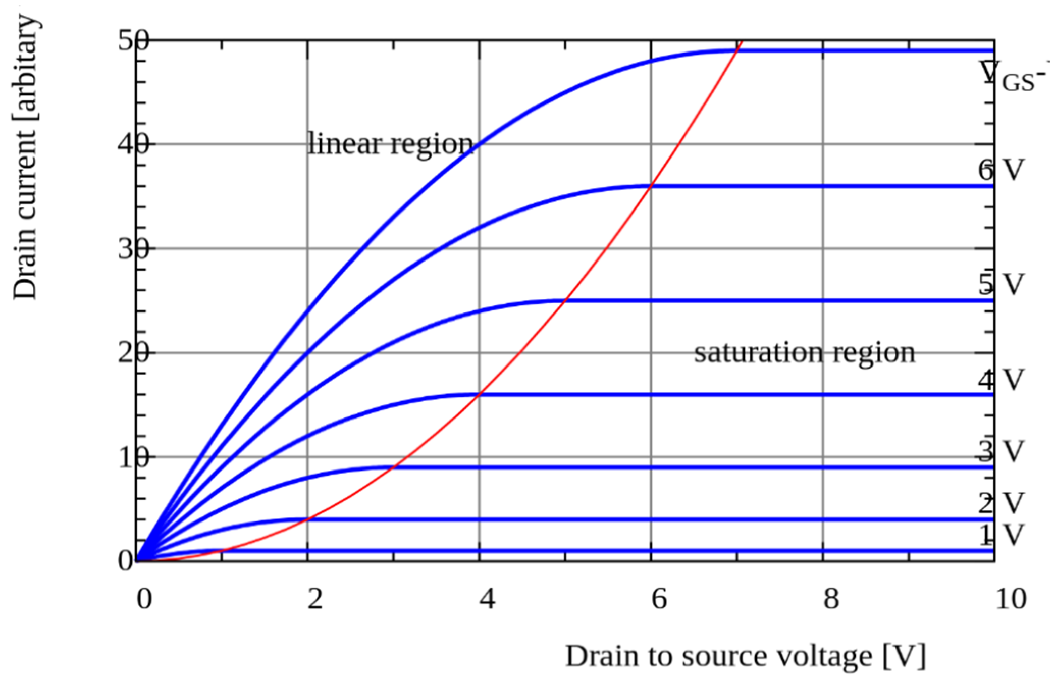
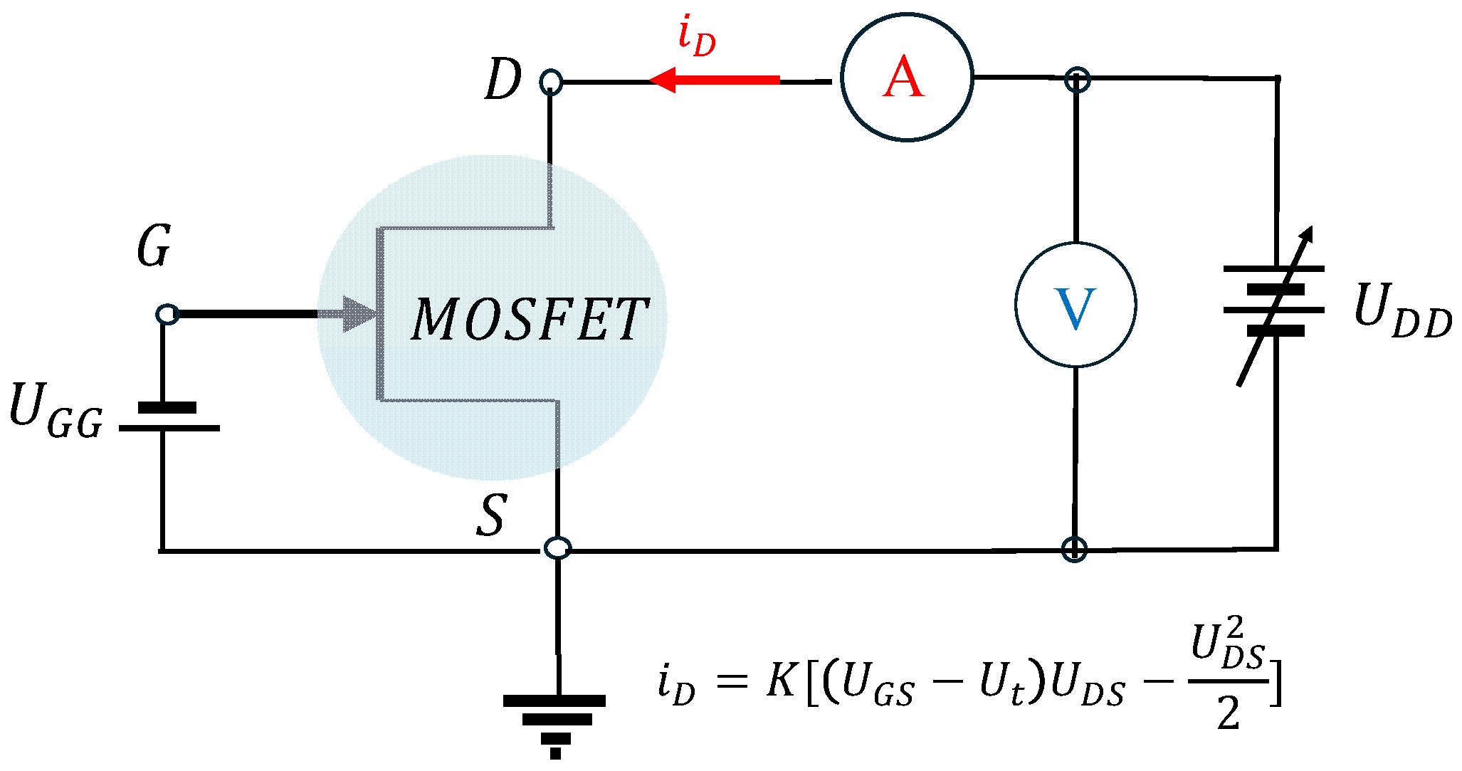
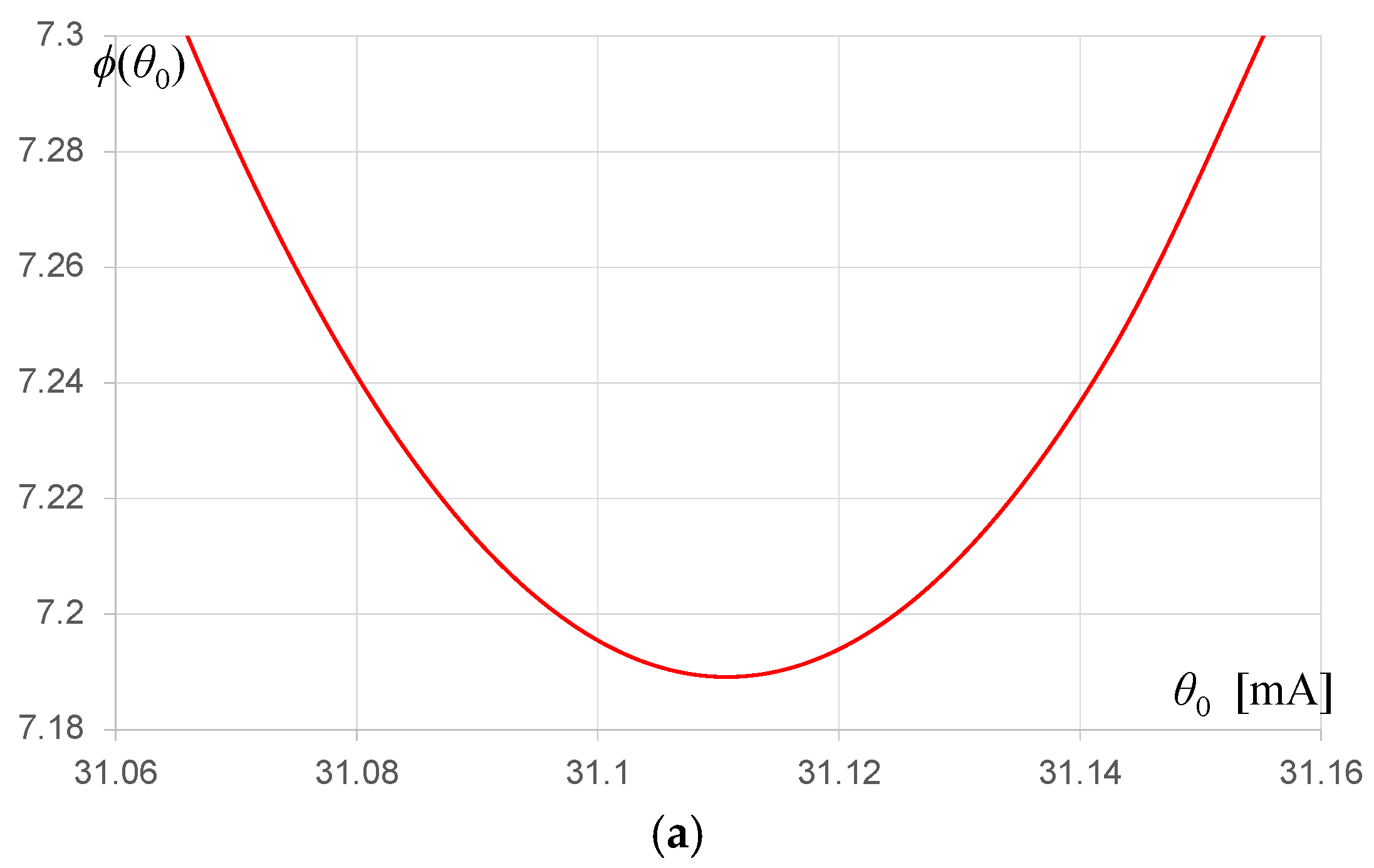
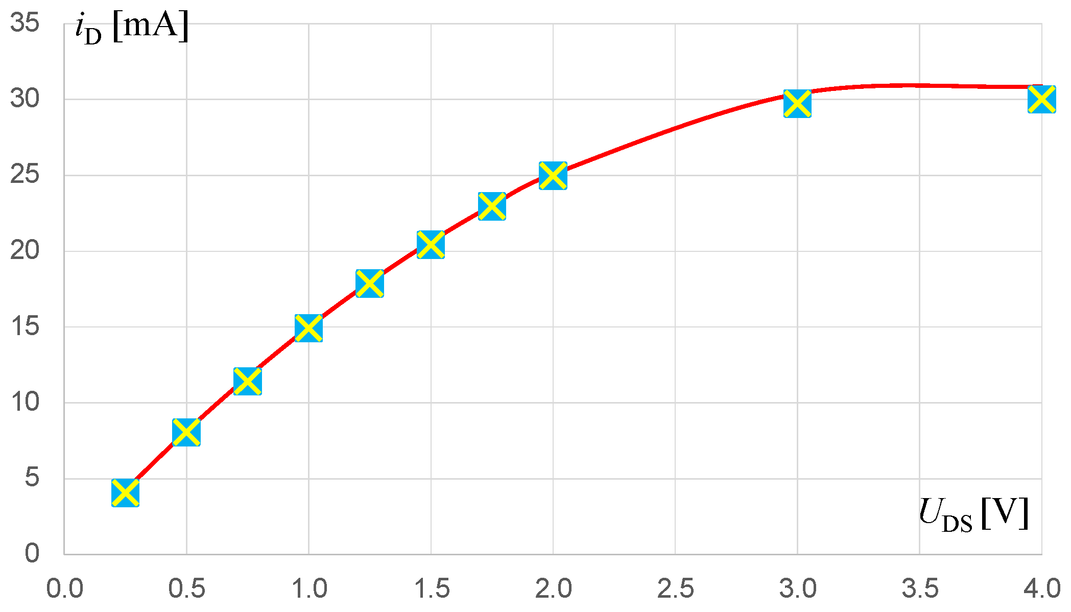
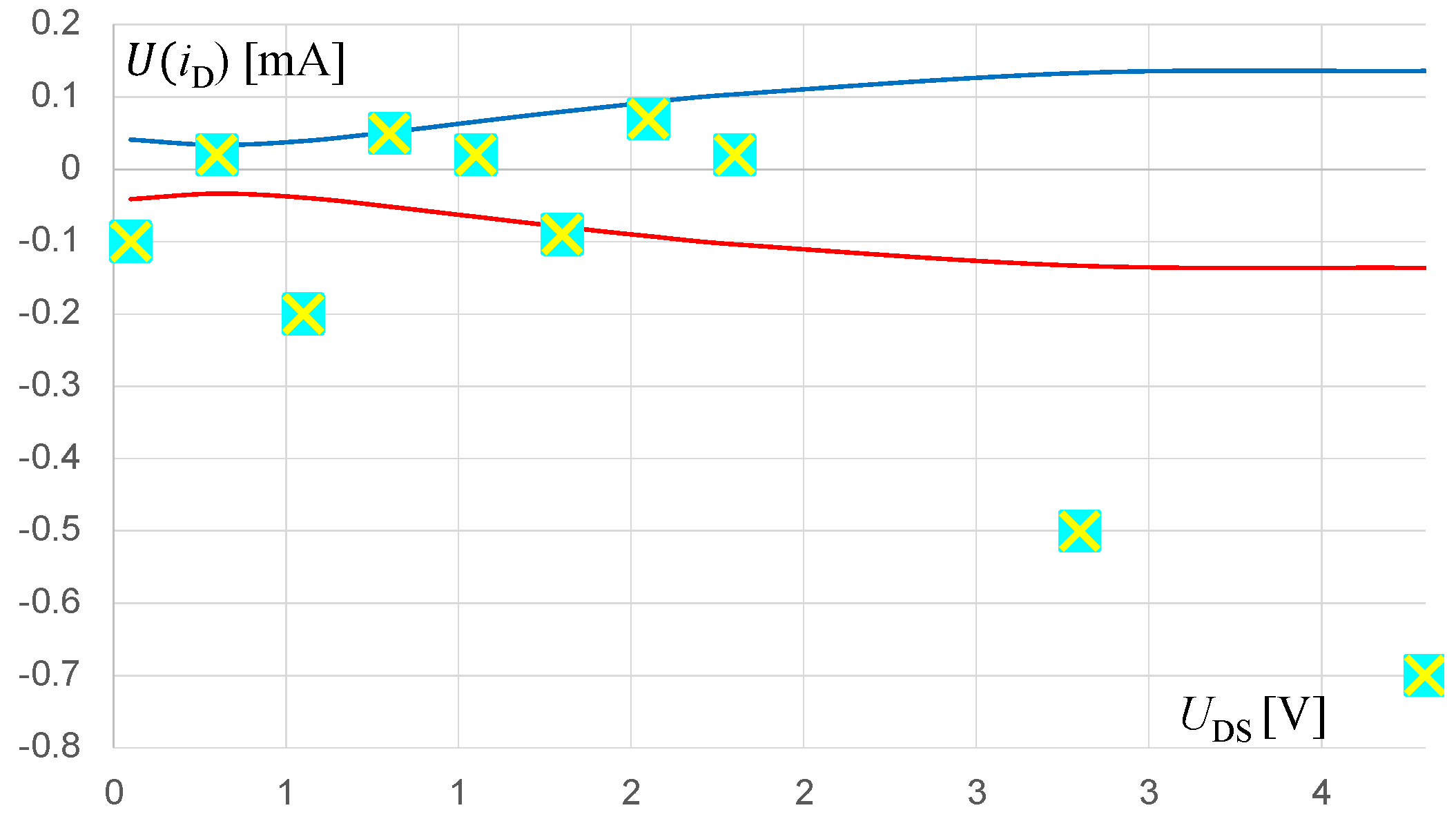
4.1. Matching the Characteristics of a MOSFET

A typical set of current–voltage characteristics of a MOSFET for the triode region is provided in Figure 7 [23].
The equation of the current iD flowing through the field effect transistor in the non-saturation range (so-called triode range) is described by the formula:
i D = K [ ( U G S U T ) U D S U D S 2 2 ]   for   U D S < U G S U T
where [mA/V2]β—transconductance coefficient—for the linear part of the characteristic has the dimension mA/V, this parameter characterizes a specific transistor; UDS, source–drain voltage; U G S , gate–source voltage; U T ,   channel creation voltage.
Measurement circuit of the current–voltage static characteristic of the transistor MOSFET BF 245 B is shown in the circuit of Figure 8.
Current iD was measured with ammeter A of 0.5% uncertainty as a function of voltage UDD measured with multi-voltmeter V with uncertainty of 0.5% for selected gate voltage U G S > U T . The transistor operated in the range of characteristics described as follows:
i D = K [ U 0 U D S U D S 2 2 ]  
where U 0 = U G S U T .
The above equation can be written in the form
i D = K 2 [ 2 U o U D S U D S 2 U 0 2 + U 0 2 ] = K ( U D D U 0 ) 2 2 + K 2 U 0 2  
In the new variables ψ ( i D ) = i D and ξ ( U D D ) = ( U D D β ) 2 , the Equation (33) becomes linear. The parameter β = U 0 is fitted. The slope coefficient θ 1 = K and free term θ 0 = K U 0 2 / 2 . The uncertainties u ( ξ ) of the new variable ξ are expressed by the formulas
u ( ξ i ) = | U D D i β | u ( U D D i )
The following values of currents and voltages obtained in the measurements are included in Table 3. For the global minimum ϕ ≈ 7.20, the fitting parameters U 0 = 6   V and   K = 4.82   mA / V 2 were obtained. The uncertainties u ( K ) and u ( K 2 U 0 2 ) , and their correlation coefficient (estimated for u(x) ≈ 0) were numerically determined as: u(K) ≈ 0.012, u ( K 2 U 0 2 ) = 0.06 and ρ = 0.97 .
In Figure 9a,b, the characteristics of the criteria function were plotted depending on the parameters θ1 and θ0 of the straight line. The fitted parabolic current–voltage characteristic of the MOSFET field-effect transistor is illustrated in Figure 10.
The width of the uncertainty corridor and the distances of measurement points from tested parabolic function are shown in Figure 11.

4.2. Measurement of a Series Connection of a Diode D and Resistor r Representing Internal Resistance of This Circuit (Type III)

To verify the proposed regression method of fitting the nonlinear curve to the measurement points, a series circuit of the connection of the semiconductor diode with the internal resistance r powered by a constant voltage power supply was considered in the arrangement according to Figure 12. Current I and voltage U are measured by ammeter A and voltmeter with relative uncertainties δ ( I ) = 0.5 % and δ ( U ) = 0.5 % respectively.
The diode is characterized by the following exponential dependence of current on the voltage measured at its terminals, using the Shockley equation
I = I 0 ( exp ( U d ε ) 1 )  
where: I 0 —is junction saturation current, ε—is constant characteristic of a particular diode and of operating temperature, and diode voltage is U d = ε   ln ( I I 0 + 1 ) .
From Kirchhoff’s second equation, it follows that the measured voltage on the two-terminal circuit connects two voltages: on the internal resistance r and across the diode junction. The current flowing through this circuit is:
I r + ε ln ( I I 0 + 1 ) = U  
Equation (36) is an implicit function
H ( I , U ) = I r + ε   ln ( I I 0 + 1 ) U = 0
because it is not possible to analytically determine the relationship of current I as a function of voltage U.
The values of the measured voltage and current at 10 measured points n = 10 of the circuit from Figure 12 are given in Table 4. Nominal parameters of such circuits are:
ε = 26   mV ,   r = 1.5   m Ω ,   I 0 = 10   μ A .
From the current and voltage measurements, we determine the resistance r , parameter ε and saturation current I 0 by adjusting the nonlinear characteristic described by (35) using the method of weighted total least squares WTLS, assuming no correlation between the measured quantities. For this purpose, we use the following substitution, which will allow us to fit both measured quantities into a straight line, as follows:
z = g ( I , U ) = U I             and                 z = θ 1 ξ + θ 0      
where θ 1 = ε , θ 0 = r and ξ = 1 I ln ( I β + 1 ) .
The measured values are transformed into new correlated coordinates: z = U/I and ξ = ln ( I / β + 1 ) / I .
Uncertainty of the new coordinate ξ ( I ) can be estimated from the law of uncertainty propagation using the first derivative of the function ξ ( I ) . Uncertainty for a variable z, from the right of propagation shall be
u ( z i ) = ( δ ( U i ) U i I i ) 2 + ( δ ( I i ) U i I i ) 2 = U i I i δ 2 ( U i ) + δ 2 ( I i )
Vectors ξ = [ ξ 1 , , ξ n ] T and z = [ z 1 , , z n ] T contain the coordinates of the measurement points after the transformation. For correlated cases with the correlation coefficient ρ ξ i z i = 1 / 2 the covariance diagonal matrix is:
[ U Y e f f ] i i = θ 1 2 u 2 ( ξ i ) + u 2 ( z i ) 2   ρ ξ i z i θ 1 u ( ξ i ) u ( z i )
Matching is based on taking a series of parameter values θ 1 , for example, with a step Δ, i.e., θ 1 j = θ 10 + ( j 1 ) Δ   and j = 1, …, 10, whereas θ 10 is the assumed initial value in which the determined values of the criterion function ϕ ξ z ( θ 1 j ) make visible the local minimum. Parameter β equals I 0 must also be preconceived. Then, when changing the range from β m i n   to β m a x , and at the same time observing the local minimum ϕ ξ z l o c a l   m i n ( θ 1 j ) , we minimize the criterion function in such a way as to obtain the global minimum ϕ ξ z g l o b a l   m i n ( θ 1 j ) . During this process, we can change both the value of the θ 10 as well as step Δ , so that the local minimum is present on the chart ϕ ξ z ( θ 1 j ) . When minimizing, there is a dependency θ 0 = ( S z θ 1 S ξ ) which determines the internal resistance r. After determining the global minimum, the parameters of the diode are:
θ 1 g l o b . m i n = ε = 26.05   mV , θ 0 g l o b . m i n = 1.50   m Ω ,   β = I 0 = 10.2   μ A   for   ϕ x z m i n = 23.46 .
Boundaries of the uncertainty corridor are presented in Figure 13. The measured points, nominal and fitted curve practically going together are given in Figure 14.

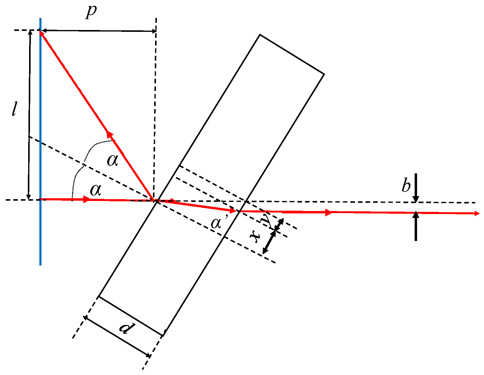
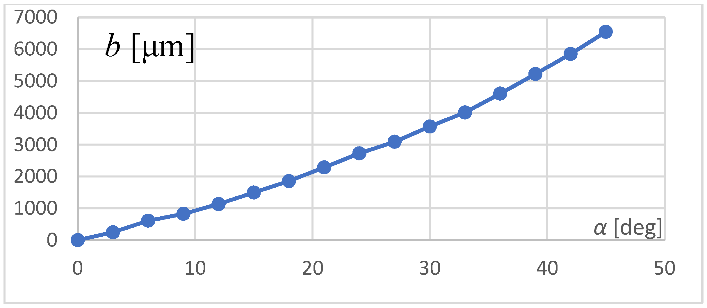
4.3. Measuring the Thickness of a Plane-Parallel Plate Using the Law of Refraction

The development of the laser in 1960 created many new measurement possibilities. The collimated laser beam is used in many non-contact measurements of geometric quantities. Figure 15 shows the principle of measuring the value of a thickness of transparent plane-parallel plate.
The laser beam falls on the plate at an angle α relative to the line normal to its surface. The laser beam partially reflects from this surface and penetrates the plate, refracting at the boundary of two media according to Snell’s law:
s i n α = 1 n s s i n α
where α is the angle of incidence relative to the normal plate surface and α’ is the angle of refraction in a medium with refractive index ns.
Then, when the laser beam leaves the plate, it is refracted again at an angle α’ with respect to the normal parallel surface of the plate, shown in Figure 15. The shift b of the laser beam axis at the system output depends on the plate thickness d and the angle of incidence α. The measured plate thickness d is described by the nonlinear relationship d = f(b, α). The measurement equation d = F(b, α) can be used to estimate the standard measurement uncertainty u(d). The linearization of nonlinear relationships can be used by changing variables and selecting the most favorable parameters of the measuring system for the range of measured plate thicknesses.
From the trigonometric relations for the course of the laser beam, we obtain:
t g α = x d ,     t g α = x + y d           and         c o s α = b y  
From (37) there is relation of y and α
y = d   t g d s i n n s 1 ( s i n n s ) 2  
After substituting relations (42) into (43) and transforming them, we obtain:
  d = b ( s i n s i n   c o s n s 2 ( s i n ) 2 ) 1
where ns—refractive index in glass.
After introducing a new variable, the following linear equations are obtained:
b = d   ξ ( α )
ξ ( ) = s i n s i n c o s n s 2 ( s i n ) 2
Measurement   equation :   d = b   ξ ( t ) 1
Error :   ε ( d ) = 1 ξ ( ) ε ( b ) b ξ 2 ( ) ε ( ξ ( ) )
Standard   uncertainty :   u ( d ) = 1 ξ 2 ( α ) u 2 ( b ) + b 2 ξ 2 ( α ) u 2 ( ξ ( α ) )
Relative   errors   ( noncorrelated ) : δ ( d ) = δ ( b ) δ ( ξ ( α ) )
where δ ( d ) = u ( d ) d , δ ( b ) = u ( b ) b , δ ( ξ ( α ) ) = u ( ξ ) ξ ( α ) .
The formula for uncertainties of the new coordinates are as follows:
u ( ξ ) = ( c o s α c o s 2 α n s 2 ( s i n α ) 2 + sin 2 2 α 4 n s 2 ( s i n α ) 2 n s 2 ( s i n α ) 2 ) u ( α )  

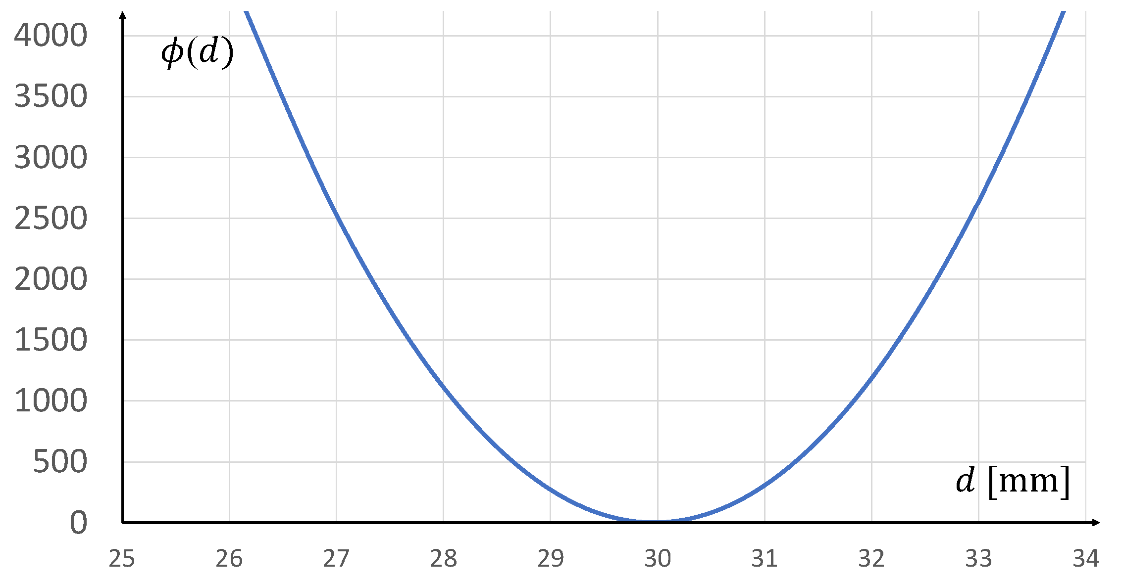
4.4. Calculation of the Measured Value d and Its Uncertainty

Measurements of one value of the plate width d can be performed multiple times at different angles of incidence α (different l). Using Formulas (40) and (41), the relationships between b and α for constant width d were calculated from data given in Table 5 and presented in Figure 16.
Measurements were also made on a plate with a thickness of d = 30 mm and with refractive index ns = 1.51 at various angles α measured with an uncertainty of 6′. The results are given in Table 6.
To determine the average value of the measurement results and its standard uncertainty, auxiliary formulas from authors’ works on linear regression [20,21] were used, for u(ξi) ≈ (6÷8) ·10−4 << ξi, (u(ξi) << u(bi)).
S = i = 1 n 1 u 2 ( b i ) ,   S ξ = i = 1 n ξ i u 2 ( b i ) ,     S ξ ξ = i = 1   n ξ i 2 u 2 ( b i ) , S ξ b = i = 1 n ξ i b i u 2 ( b i ) ,   S b = i = 1 n b i u 2 ( b i ) ,
Δ = S S ξ ξ S ξ 2
For d0 = 0, and u ( d 0 ) = S ξ ξ / Δ is obtained d = ( S S ξ b S ξ S b ) / Δ .
From data in Table 6 the average value: d ≈ 29.97 mm and standard uncertainties of parameters of measurement system: u(b) = 0.01mm, u(α) = 6′, u(ξ) = (6÷8) ·10−4 ≈ 0, was determined.
The WTLS criterion function obtained is provided in Figure 17. It is practically a parabola with a minimum of d = 30.00 mm. Standard uncertainty of the measurement result obtained was u(d) = S / Δ ≈ 0.06 mm. Result of measurements of plate thickness obtained were d = (29.97 ± kp 0.06) mm (for the probability P = 0.95 of Gauss distribution the coefficient kp = 2).
The above example of the laser measurement system relates to measuring the thickness of transparent plane-parallel plates with dielectric layers applied. Some of these plates cannot be measured using contact methods and as such must use non-contact optical methods. A collimated laser beam of continuous radiation and the law of light refraction on both parallel surfaces of the plate were used.
The accuracy of measuring the thickness of a transparent plate according to the principle presented in Figure 15 can be increased by performing measurements at many different values of the angle α of incidence of the beam on the plate. Formulas for relative uncertainties are also provided. It is possible to determine nonlinear functions F(d, b) for specific angles α using the linear regression method and their uncertainty bands to select the most favorable variant for measuring a specific value of width d.

5. Conclusions

This paper presents a method of fitting nonlinear curves to data of measured points and estimating their uncertainty band.
The change of variables to new ones to obtain the linear relationship and the WTLS total least squares criterion was used. This method considers influences of coordinates of measured points and their uncertainties and auto-correlation and mutual correlations of these coordinates’ observations. It involves replacing the function of nonlinear relationship between coordinates x, y with a linear relationship of the new Cartesian coordinates ξ ,   ψ after transformation.
The method proposed in this paper allows us to find optimal parameters of the nonlinear functions fitted to the measurement data.
The condition for using this method is permissible approximation of the errors and uncertainties propagated by the first derivative of the transformation function.
This work also describes a few numerical examples containing transformation of one and both coordinates of a measurement function, as well as for implicit function.
The calculations obtained lead to the conclusion that this method can be used to fit most of the different nonlinear functions to given data of measurement points and find their uncertainty band (uncertainty corridor) with satisfying accuracy.
This method is an analytical one with numerical optimization of parameters of the nonlinear function fitted to measure data of tested points. It is simpler than other methods used for fitting nonlinear functions including artificial neural networks (ANN) methods.
This novel method proposed by the first two authors may be very useful in routine measurement practice and should be considered in the development of the new version of the GUM guide [19] considering its relevance to the evaluation of the parameters and uncertainty bands of different nonlinear functions describing measurements.

Author Contributions

Methodology, Z.L.W.; Formal analysis, T.W.; Writing—original draft, J.P. This novel analytical method of fitting the nonlinear function to data of measurement, was proposed by Z.L.W. and J.P. in 2022/23 [20,21,22], Example 4.3 of this method application in optical measurement is given by third author T.W. All authors have read and agreed to the published version of the manuscript.

Funding

The researchers did not receive any specific grant from funding agencies in the public, commercial, or non-profit sectors.

Data Availability Statement

Data is contained within the article.

Conflicts of Interest

The authors declare no conflict of interest.

References

  1. Joint Committee for Guides in Metrology (BIPM, IEC, IFCC0, ILAC, ISO, IUPAC, IUPAP & OIML). JCGM 100:2008 Evaluation of Measurement Data—Guide to the Expression of Uncertainty in Measurement, and its Supplements; International Bureau of Weights and Measures BIPM: Sevres, France, 2008. [Google Scholar]
  2. Levenberg, K. A Method for the Solution of Certain Non-Linear Problems in Least Squares. Q. Appl. Math. 1944, 2, 164–168. [Google Scholar] [CrossRef]
  3. Marquardt, D. An Algorithm for Least-Squares Estimation of Nonlinear Parameters. SIAM J. Appl. Math. 1963, 11, 431–441. [Google Scholar] [CrossRef]
  4. Dennis, J.E., Jr.; Schnabel, R.B. Numerical Methods for Unconstrained Optimization and Nonlinear Equations; SIAM 1996 Reproduction of Prentice-Hall: New York, NY, USA, 1983. [Google Scholar]
  5. Draper, R.D.; Smith, H. Applied Regression Analysis, 3rd ed.; Wiley: New York, NY, USA, 1998. [Google Scholar]
  6. Kanzov, C.H.; Yamashita, N.; Fukushima, M. Levenberg–Marquardt methods with strong local convergence properties for solving nonlinear equations with convex constraints. J. Comput. Appl. Math. 2004, 172, 375–391. [Google Scholar] [CrossRef]
  7. Madsen, K.; Nielsen, H.B. Tinglef. Method for Non-Linear Least Squares Problems, 2nd ed.; Informatics and Mathematical Modelling, Technical University of Denmark: Lyngby, Denmark, 2004. [Google Scholar]
  8. Krystek, M.; Mathias, A. A least-squares algorithm for fitting data points with mutually correlated coordinates to a straight line. Meas. Sci. Technol. 2011, 22, 035101. [Google Scholar] [CrossRef]
  9. Amiri-Simkooei, A.R.; Jazaeri, S. Weighted total least squares formulated by standard least squares theory. J. Geod. Sci. 2012, 2, 113–124. [Google Scholar] [CrossRef]
  10. Grafarend, E.W.; Awange, J.L. Applications of Linear and Nonlinear Models—Fixed Effects, Random Effects, and Total Least Squares. J. Geod. Sci. 2013, 3, 77–78. [Google Scholar] [CrossRef]
  11. Christodoulos, A.; Par Floudalos, M. Encyclopedia of Optimization; Springer: Berlin/Heidelberg, Germany, 2008; p. 1130. ISBN 978038774583. [Google Scholar]
  12. Mascarenha, S.W.F. The divergence of the BFGS and Gauss Newton Methods Math. Programming 2013, 147, 253–276. [Google Scholar] [CrossRef]
  13. Gulsen, M.; Smith, A.E.; Tate, D.M. A Genetic Algorithm Approach to Curve Fitting. Int. J. Prod. Res. 1995, 33, 911–933. [Google Scholar] [CrossRef]
  14. Denison, D.G.T.; Mallic, B.K.; Smith, A.F.M. Automatic Bayesian Curve Fitting. Journal of the Royal Statistical Society. Ser. B (Stat. Methodol.) 1998, 60, 333–350. [Google Scholar] [CrossRef]
  15. Karr, C.L.; Weck, B.; Massart, D.L.; Vankerbergh, P. Least Median Squares Curve Fitting Using a Genetic Algorithm. Eng. Appl. Artif. Intell. 1995, 8, 177–189. [Google Scholar] [CrossRef]
  16. Tellinghuisen, J. Least Squares Methods for Treating Problems with Uncertainty in x and y. Anal. Chem. 2020, 92, 10863–10871. [Google Scholar] [CrossRef] [PubMed]
  17. Li, M.; Verma, B. Nonlinear Curve Fitting to Stopping Power Data Using RBF Neural Networks. Expert Syst. Appl. 2016, 45, 161–171. [Google Scholar] [CrossRef]
  18. Li, M.; Li, L.D. Novel Method of Curve Fitting Based on Optimized Extreme Learning Machine. Appled Artif. Intell. 2020, 34, 849–865. [Google Scholar] [CrossRef]
  19. Klauenberg, K.; Martens, S.; Bošnjaković, A.; Cox, M.G.; Van der Veen, A.M.H.; Elster, C. The GUM perspective on straight-line errors-in-variables regression. Measurement 2022, 187, 110340. [Google Scholar] [CrossRef]
  20. Puchalski, J.; Warsza, Z.L. Assessment of the uncertainty of selected nonlinear functions determined from measurements by the linear regression method. In Advanced Mathematical and Computational Tools in Metrology and Testing XIII; Series on Advances in Mathematics for Applied, Sciences; Pavese, F., Bošnjaković, A., Eichstädt, S., Forbes, A.B., Alves e Sousa, J., Eds.; World Scientific Publishing Co.: New York, NY, USA; London, UK; Singapore, 2024; Volume 94, pp. 288–307. [Google Scholar] [CrossRef]
  21. Puchalski, J.; Warsza, Z.L. The method of fitting a non-linear function to data of measured points and its uncertainty band. Pomiary Automatyka Robotyka PAR. n3_2023. pp. 45–55. Available online: https://par.pl/Archiwum/2023/3-2023/Metoda-dopasowania-funkcji-nieliniowej-do-danych-punktow-pomiarowych-i-jej-pasmo-niepewnosci (accessed on 12 November 2024). (In Polish).
  22. Puchalski, J.G. Nonlinear Curve Fitting to Measurement Points with WTLS Method Using Approximation of Linear Model. Int. J. Auto. AI Mach. Learn. 2024, 4, 36–60, ISSN 2593-7568. [Google Scholar] [CrossRef]
  23. MOSFET Physics. Available online: https://www.mks.com/n/mosfet-physics (accessed on 1 January 2020).
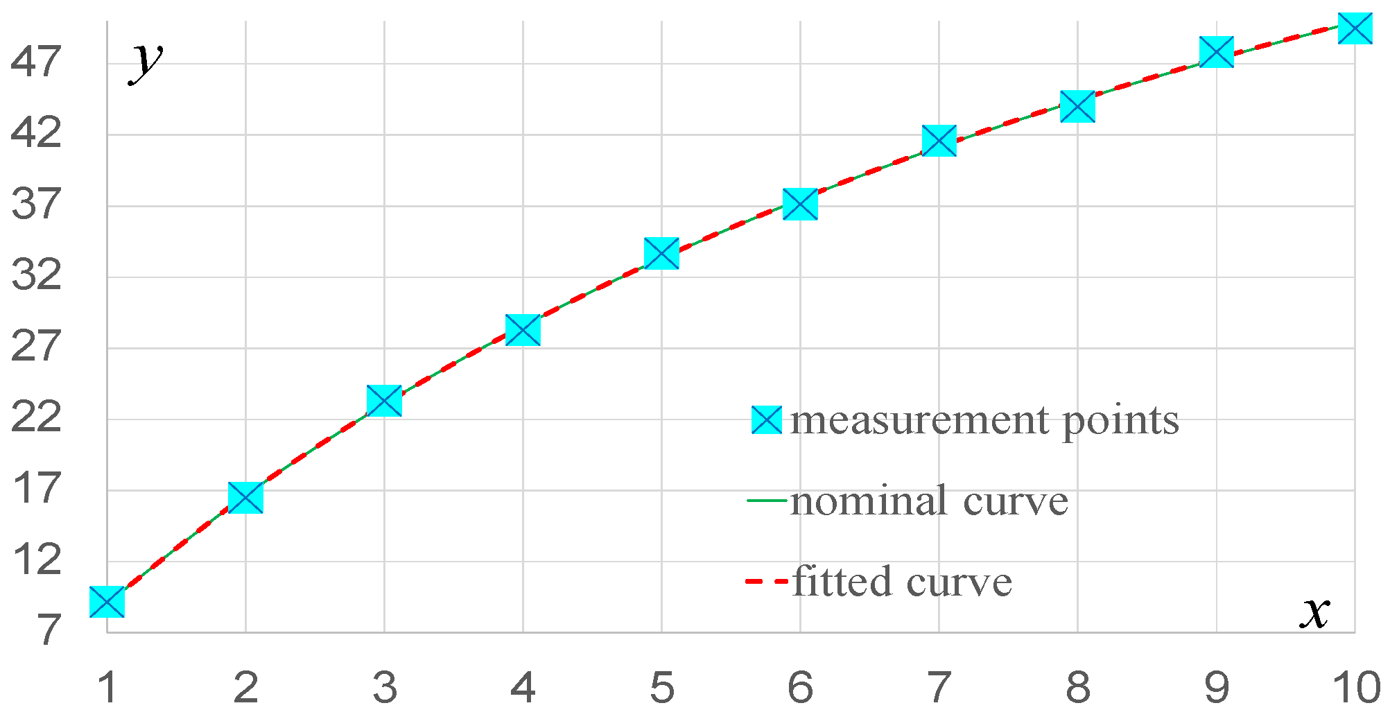
Figure 1. Examples of typical characteristics of criterial function ϕ ξ ψ with local (red line) minimum and global minimum (red dot).
Metrology 04 00042 g001
Figure 2. Quasi-parabolic numerical characteristics: (a) ϕ ξ ψ ( θ 1 ), (b) ϕ ξ ψ ( θ 0 ) for β m i n = 0.66, ϕ ξ ψ m i n ≈ 67.39.
Metrology 04 00042 g002
Figure 3. Parabola fitted to data of the test points x from Table 1: (a) with correlation, (b) without correlation—dashed blue line and its uncertainty band for coverage 0.95—finely dashed red lines.
Metrology 04 00042 g003
Figure 4. Expanded uncertainties U and deviation Δf of the fitted characteristic from the nominal one, for correlated and uncorrelated quantities measured as functions of the x coordinate.
Metrology 04 00042 g004
Figure 5. Nominal nonlinear curve together with fitted curve y = x 0.01 x + 0.1   at   the   level     ϕ ψ ξ m i n ≈ 1.72.
Metrology 04 00042 g005
Figure 6. Measurement points, the error between fitted and nominal curve and expanded uncertainty band Uy of curve fitted to noncorrelated measurements from data given in Table 2.
Metrology 04 00042 g006
Figure 7. Characteristics of the drain current as a function of the source–drain voltage for different voltages between the gate and the source.
Metrology 04 00042 g007
Figure 8. Measuring circuit layout for determining parameters and the static characteristics of the MOSFET transistor.
Metrology 04 00042 g008
Figure 9. Characteristics of the dependence of criterion function on global minima depending on the parameter: (a) θ 1 , (b) θ 0 .
Metrology 04 00042 g009aMetrology 04 00042 g009b
Figure 10. Measuring points and the fitted parabolic current–voltage characteristic of the MOSFET field-effect transistor.
Metrology 04 00042 g010
Figure 11. Distances to measurement points and uncertainty corridor for the current—voltage characteristics of the MOSFET field-effect transistor.
Metrology 04 00042 g011
Figure 12. Measurement system for the determination of nonlinear matched characteristics U(I) to the measuring points.
Metrology 04 00042 g012
Figure 13. Distances of measurement points from curve fitted to their data and uncertainty band of noncorrelated measurements from data are shown in Table 4.
Metrology 04 00042 g013
Figure 14. Measurement points, nominal nonlinear curve and fitted curve with parameters: ε = 26.04   mV , r = 1.5 mΩ, I 0 = 10.2   μ A ,   at   the   level   ϕ x z m i n  ≈ 23.46.
Metrology 04 00042 g014
Figure 15. Scheme of laser thickness measurement of a transparent plane-parallel plate.
Metrology 04 00042 g015
Figure 16. Dependence of the measured output parameter b on the angle of incidence α of the beam.
Metrology 04 00042 g016
Figure 17. Dependence of the criterion function on parameter d.
Metrology 04 00042 g017
Table 2. Coordinates of measurement points for function (14).
x12345678910
y9.1816.5023.3128.2933.6737.1341.5944.0047.8449.50
Table 1. Coordinates of the examined points of the second-degree parabola with parameters rated A = 2; B = 3; C = 4 and their deviations Δy to the nominal parabolic characteristic.
No.Coordinates of Measurement PointsMatching Errors to Nominal
Parabolic Characteristic
Δy [V]
xi [V] y i [V]
12.7910.00−1.00
27.1317.50 0.50
313.4735.00−4.00
421.8146.00 2.00
532.1571.00−2.00
644.4997.00−3.00
758.83122.00 1.00
875.17158.00−2.00
993.51194.00−1.00
10113.85232.00 2.00
Table 3. Value of voltages and currents obtained from measurements at circuit shown in Figure 8.
i D (mA)0.250.50.7511.251.51.75234
U D S ( V ) 4.078.0611.4114.9317.8720.4822.9624.9829.7430.02
Table 4. The coordinates of measurement points given by measurement site—Figure 12 [23].
I (mA)1.101.373.296.8021.9869.09148.75317.59970.121975.35
U (mV)120130150170200230250270300320
Table 5. Parameter b for different angles α of laser beam.
α [deg]0369121518212427303336394245
b [μm]0247.9609.7824.11132.31494.11855.92284.72726.93088.73571.14013.34602.95219.35849.16545.9
Table 6. Results of measurements of parameter b for various angles α when d = 30 mm.
α [rad]0.050.100.150.200.250.300.350.400.450.50
b (mm)0.511.021.532.062.593.153.724.314.925.56
Disclaimer/Publisher’s Note: The statements, opinions and data contained in all publications are solely those of the individual author(s) and contributor(s) and not of MDPI and/or the editor(s). MDPI and/or the editor(s) disclaim responsibility for any injury to people or property resulting from any ideas, methods, instructions or products referred to in the content.

