Study of the Errors in Interpolated Fast Fourier Transform for Interferometric Applications

Abstract

Frequency estimation is often the basis of various measurement techniques, among which optical distance measurement stands out. One of the most used techniques is interpolated fast Fourier transform due to its simplicity, combined with good performance. In this work, we study the limits of this technique in the case of real signals, with reference to a particular interferometric technique known as self-mixing interferometry. The aim of this research is the better understanding of frequency estimation performances in real applications, together with guidance on how to improve them in specific optical measurement techniques. An optical rangefinder, based on self-mixing interferometry, has been realized and characterized. The simulation results allow us to explain the limits of the interpolated fast Fourier transform applied to the realized instrument. Finally, a method for overcoming them is proposed by decorrelating the errors between the measurements, which can provide a guideline for the design of frequency-modulated interferometric distance meters.

1. Introduction

In various measurement systems, the physical variable of interest is the frequency of a signal. In electronics and telecommunications fields, there is a great variety of examples requiring tone detection, such as the correct estimation of electricity network frequency as the main quality parameter in power systems [1], the detection of Doppler tones in radar systems [2], or in different measurement systems, where the sensor’s output is a signal frequency, for example a quartz resonator [3], fiber-optic voltage sensor [4] or silicon vibrating sensor [5]. Optical instruments based on the Doppler effect are well-known non-contact measurement systems for distance or vibration measurements [6]. By definition, relative motion between a source that generates a wave and the observer who is receiving the wave leads to a change in the frequency of the wave, known as the Doppler effect. This implies that the Doppler effect-based measurement systems are developed upon the frequency measurement. In the case of vibration measurement, the working principle is based on the interference observed when two coherent light beams are made to coincide. The resulting intensity, measured by a photodetector, varies as a sinusoidal function of the phase difference between the two beams. Considering a moving target, the scattered back beam by the target’s motion is subjected to a frequency shift, called Doppler shift. Such a frequency modulation of the light intensity is proportional to the vibration velocity [6].

Absolute distance, on the other hand, can be obtained by modulating the wavelength of the laser source where the frequency of the interferometric fringes is proportional to the distance to the target [7]. Despite high resolution in distance measurement systems based on interferometric techniques, complicated and costly optical setup limits the industrial applications of such techniques. As an alternative approach, the self-mixing interference effect in a laser diode has led to widespread measurement applications with high resolution while remaining very small in size and cost-effective.

Self-mixing interferometry (SMI) is a well-established optical technique that leverages the optical back-injection phenomenon occurring within a laser cavity [8]. When a small portion of the emitted power is reflected into the laser diode, it induces modulation in both the emitted power and frequency [9]. In cases where a photodiode is positioned behind the laser cavity (often referred to as a monitor photodiode), it can directly measure the power modulation. This modulation takes on a periodic waveform F(φ) = F(4πs/λ), which is influenced by the laser wavelength (λ) and the target distance (s). The shape of F(φ) closely resembles a sinusoidal waveform when the back reflection is minimal (below 10⁻⁸ in power), but it becomes distorted as the optical feedback increases. 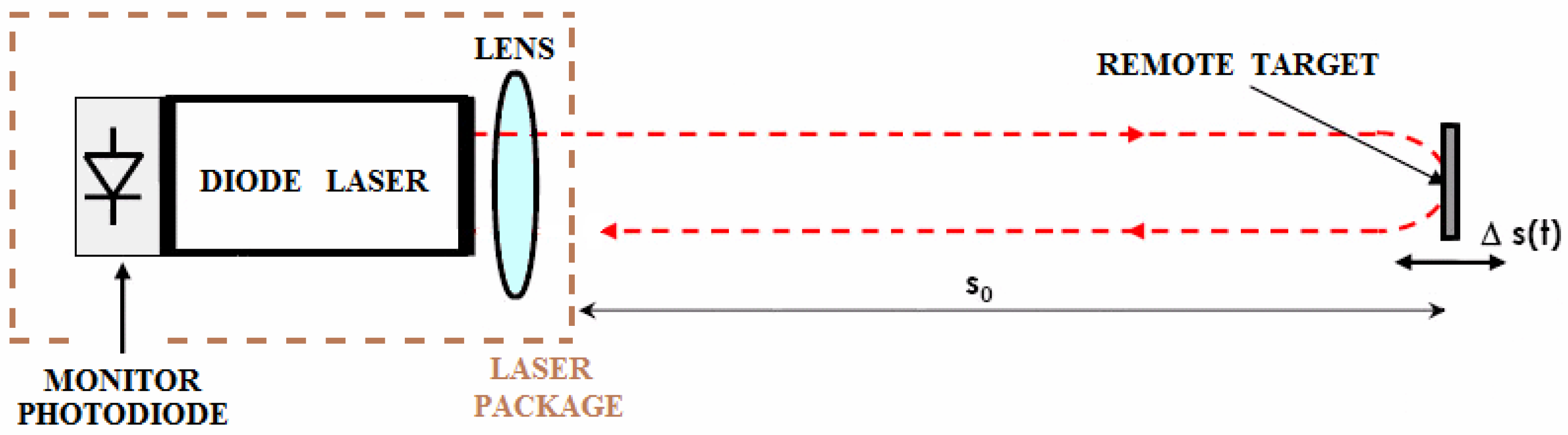The feedback intensity is measured by the C parameter [9]. A typical setup for a self-mixing interferometer [10] is depicted in Figure 1 where it can be limited to the laser diode with a monitor photodiode and a focusing lens.

As an attractive feature, SMI can work even with very low returning power (e.g., 10⁻⁸ of laser power) resulting in triggering many measurement applications. There is also the possibility to improve the SMI signal-to-noise ratio by applying a sort of balanced detection [11], or by reading the frequency modulation with more complex schemes [12]. In the field of fluid dynamics, self-mixing interferometry can be used in flow measurement applications. In the SMI-based flow measurement system, flow velocity is determined through the Doppler shift induced by the scattering particles inside the fluid [13], with the possibility to measure the flow profile [14], even through an array of lasers [15]. In applications such as motion analysis and speed measurement [16], analyzing the Doppler shift in the self-mixing signal using phase-unwrapping techniques [17] is also relevant for Mechatronics Applications [18] or acoustic emission measurement [19]. The interference signal can be influenced by vibrations [20], making self-mixing interferometry suitable for vibration measurement to monitor structural vibrations and analyze mechanical systems [21]. Different techniques can be applied to determine the vibration. For instance, it can be reconstructed directly from the fringes signal, without any electronic feedback (open-loop) or it can be done by employing feedback to the laser pump current (closed-loop), to lock the SMI in a fringe center [22]. As highlighted above, the frequency of the interference signal generated by the interaction of the laser beam with the target is essential for extracting valuable parameters and characteristics in various applications.

In this work, we focus on frequency estimation techniques for SMI-based measurement systems. The aim of this research is to understand the limits of these techniques in real signals, and to propose a method for overcoming these limits. The rest of the paper is organized as follows. Section 2 discusses various single-tone frequency measurement techniques in addition to a comprehensive comparison. Despite the simplicity and reliability of the interpolated fast Fourier transform (IFFT), Section 3 addresses the errors in the IFFT while it is applied to a practical measurement case study based on self-mixing interferometry, as discussed in Section 4. Finally, the results and conclusion are presented in Section 5 and Section 6, respectively.

2. Single-Tone Frequency Measurement Techniques

In the literature, a large number of techniques can be found for the accurate measurement of signal frequency. The digital elaboration, indeed, allows to simplify the frequency analysis thanks to the implementation of different kinds of algorithms [23,24,25]. The aim of this work is to study the limits of the estimation techniques on the frequency of a real interferometric signal. In the following, we present the most widespread techniques for frequency estimation, trying to underline their strengths and weaknesses for this particular application.

In general, given a sinusoidal signal A(t) = A₀ · sin(2πft + φ), the quality of the exact frequency estimation depends both on the time acquisition window, and on the signal-to-noise ratio of the original signal. In some cases, the estimation is made by the direct measurement of the time interval through two consecutive zero crosses, with the same slope. However, this technique is suitable only when the tone is noiseless and at low frequency compared to the time base clock. In order to realize a robust detection algorithm, it is better to operate in the frequency domain by evaluating the Discrete Fourier Transform (DFT) of the signal. With the DFT, the spectral resolution Δf_bin is limited to Δf_bin = f_samp/N value, where f_samp is the sampling rate of the acquired signal and N is the number of acquired samples. It is easy to demonstrate that Δf_bin is equal to the inverse of the acquired time window. This indicates a limit in the frequency resolution; the details in the spectrum are masked by the temporal duration of the processed signal and by the window type used in order to reduce the spectral leakage [24]. Nevertheless, under the assumption that the signal contains a main tone at constant frequency, it is possible to overcome the limited resolution of the DFT in order to accurately evaluate only the tone frequency, not all the spectral content. There are known methods to realize this kind of measurement [26]. A typology of tone detection is the interpolated FFT (IFFT) [23], consisting of the elaboration of the standard FFT by some interpolating equations between adjacent bins to better estimate the mean tone frequency. The IFFT method has the advantage of low computational complexity and is, thus, commonly used in measurement systems, but the result is only an approximation of the signal main tone.

A completely different way of elaboration is the so-called Zoom Fast Fourier Transform [27], often used in digital spectrum analyzers; through a series of complex multiplications, low-pass filtering, decimations and FFT, this algorithm performs an expansion of the original spectrum, allowing for a better estimation of the tone frequency. This technique is useful when there is the need to zoom a particular section of spectrum, but it is limited in terms of frequency resolution.

Finally, another powerful technique for enhancing the spectral resolution is known in the literature as Chirp Z-Transform (CZT) [28]. From a discrete signal of N points, this method evaluates the Z-transform at M points, in the Z-plane, which lie on circular or spiral contours beginning at any arbitrary point in the Z-plane. The angular spacing of the points is an arbitrary constant, and N and M are integers. In other words, under particular conditions, it is possible to calculate a zoomed spectrum of the sequence from an arbitrary start frequency and span, and then to evaluate a more accurate frequency peak of the main tone. The CZT offers more flexibility than a DFT for many reasons: the number of time samples does not have to be equal to the number of samples of the Z-transform, N and M do not need to be a composite integer and, finally, the step frequency and the starting frequency are arbitrary. In other words, if a pure sinusoidal signal with frequency f₀ is processed by common DFT, it results in a peak (or a series of peaks in the case of bin-leakage) in the magnitude representation at the position f₀; but if the CZT is used in a frequency range between the first two lateral lobes of the cardinal sine |sin(f − f₀)/(f − f₀)| shape (due to a rectangular windowing), a zoomed spectrum is evaluated. 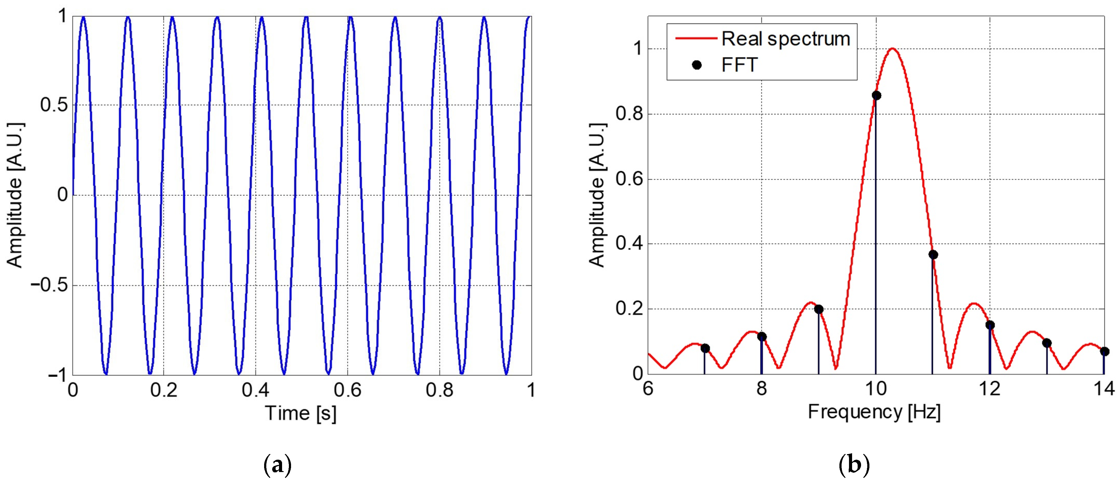Figure 2 shows an explanation of the working principle; if the sampled signal is a pure sinusoid (Figure 2a), trunked at 1 s, its spectrum is the cardinal sine reported in Figure 2b, while the DFT of the signal acquired for 1 s has a resolution limited to 1 Hz. With this ideal signal, the CZT finds the signal frequency as the index of the maximum of the cardinal sine. The estimation accuracy of the maximum (CZT) is clearly better than the resolution-limited DFT. However, the calculus of the CZT involves a complex convolution and two complex multiplications [28]; therefore, the implementation on a portable device, like a DSP processor, may be critical and time-consuming.

The other most employed technique for estimating the frequency of a signal is the interpolated FFT (IFFT). Referring to [23,29], the IFFT allows measurements with good trade-off between accuracy and computational cost. The principle of operation of the IFFT consists of three steps: first, the acquired signal is multiplied by a Hann window; second, the magnitude DFT is evaluated; finally, the frequency estimation is obtained by solving an equation that correlates some DFT bins. In particular, given the spectrum magnitude of the signal, the frequency estimation f_est of the main tone may be calculated by an interpolation, known as two-point IFFT (1):

$$f_{est}=\left(m_{max}\pm \frac{2\cdot h_{m\pm 1}-h_m}{h_{m\pm 1}+h_m}\right)\cdot \frac{f_{samp}}{N},$$

(1)

where f_samp is the sampling rate of the input signal, N is the number of acquired samples and m_max is the higher bin index of the DFT, with value h_m. The sign of the inner sum depends on the amplitude comparison of the lateral bin; if the right bin h_m+1 is greater than h_m−1, ‘+’ will be used, otherwise ‘−’.

The intrinsic error committed by (1) is due to the linearization of the transcendent shape of the spectrum, which reaches its maximum between two consecutive bins. Considering the simplicity of adding (1) to an FFT computation, the IFFT is widely used in different real-time applications such as, for example, in [30].

Many other techniques of particular spectral analysis are described in the literature, also for power quality frequency assessment [31]. The Warped Discrete-Fourier Transform (WDFT) [32], for example, has frequency samples allocated nonuniformly over the unit circle, allowing for the development of different FIR filters. The spectral analysis for power electronics has been realized with different variants of CZT, the Adaptive Chirp Transform (ACT) [33], or the Segmented Chirp Z-Transform (SCZT) [34].

Considering self-mixing interferometry, where the interference signal may contain multiple frequency components or harmonics, a powerful tool such as the Multiple Signal Classification (MUSIC) algorithm can be employed to estimate these frequencies [35]. The MUSIC algorithm is a spectral estimation method used for identifying the frequencies present in a signal. It is particularly powerful in the presence of multiple signals or closely spaced frequencies. Estimating the frequency of a sinusoidal signal, especially in the presence of noise, can be achieved through the ALL-PHASE technique. It helps mitigate the impact of noise and other disturbances on the accuracy of frequency determination, which is crucial in applications such as distance measurement, velocity measurement, and vibration analysis. In [36], an ALL-PHASE FFT method is proposed for distance measurement while dealing with SMI signals to suppress the influence of spectrum leakage and signal noise in addition to reducing computational time appropriately.

In this paper, we will focus on the IFFT due to its lower complexity and reliability in the majority of real-time applications.

3. Interpolated FFT Errors

Depending on the window used, there are different interpolation techniques. For example, (1) is valid only for the Hann window. In [37], a deep study of the accuracy in the IFFT as a function of interpolation technique is reported, but it does not include the limits typical of real signals: the presence of noise and the possibility that the signal is not a pure sinusoid. The results of various simulations are reported below, carried out considering a sampling frequency of 8.4 MSPS, in order to be able to make a direct comparison with the experimental results shown in Section 4. The sampling frequency set is the highest possible with the embedded electronics used (microcontroller model STM32F4).

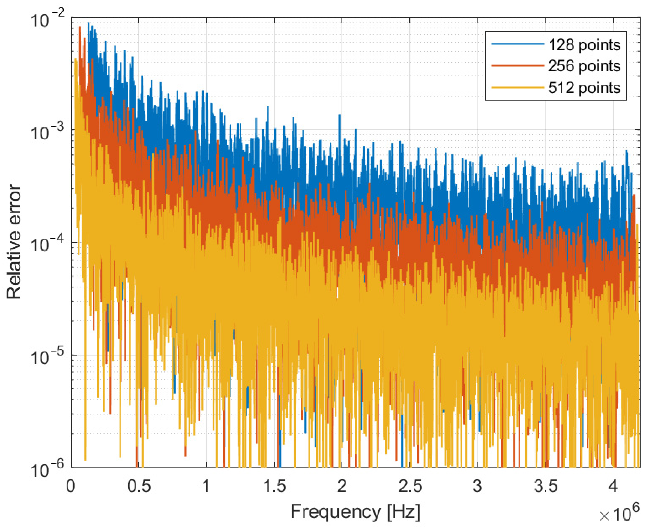
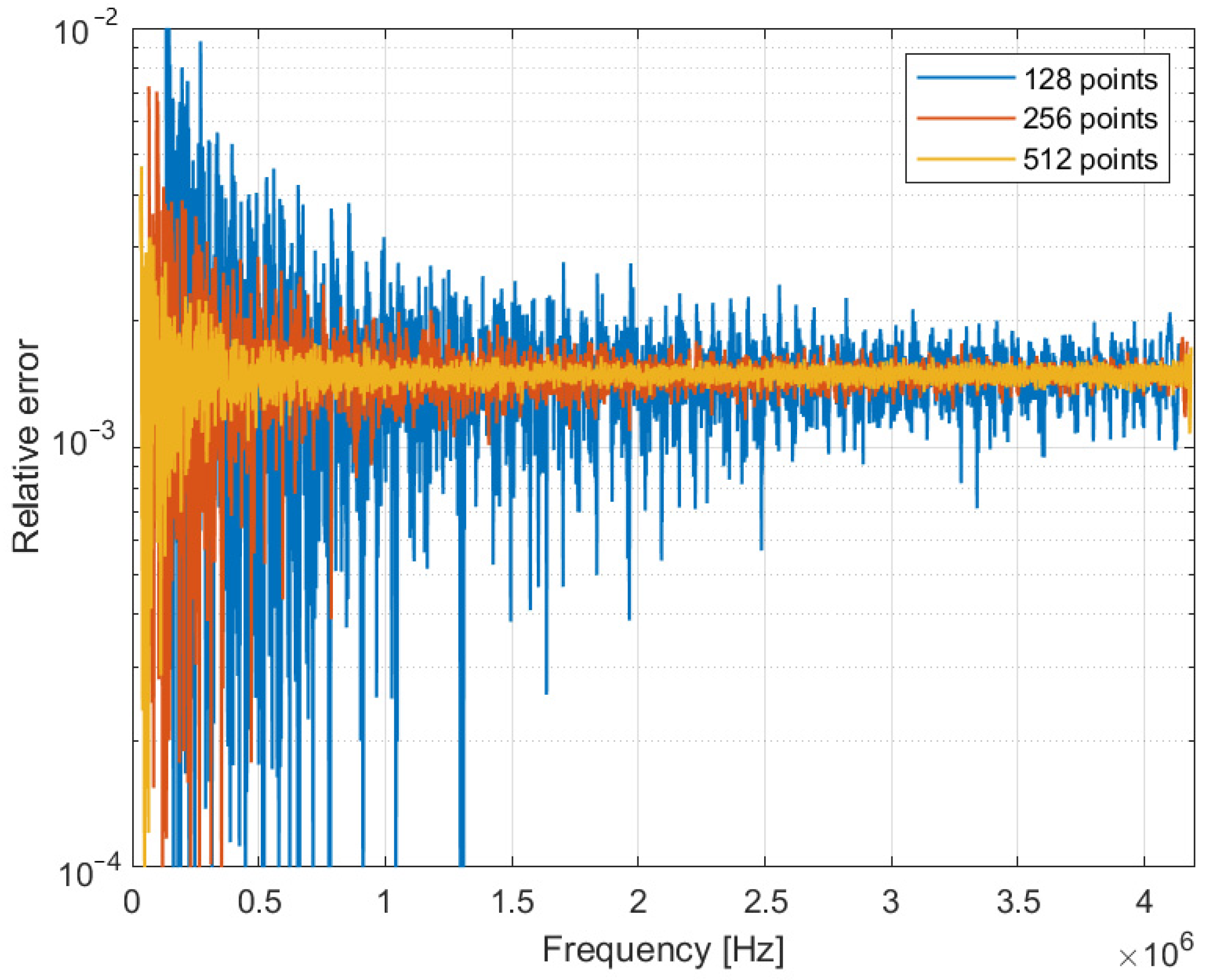
The first simulation calculates the error in the frequency estimation made by the two-point IFFT as a function of the signal frequency. The simulated signal is a pure sine wave, sampled at 8.4 MSPS with different acquisition lengths. Figure 3 compares the calculated relative error given by the two-point IFFT, evaluated on 128, 256 and 512 samples. The choice of this limited number of samples is linked to implementation needs of real-time measurement systems. The maximum sampling rate does not allow acquiring an arbitrary number of points, considering the measurement speed requirements. As expected, the simulation results confirm the progressive improvement with the number of samples in this ideal condition.

In a real case, even if the signal is a pure sine, the presence of noise reduces the IFFT accuracy. Figure 4 shows an example of simulation in the case of a pure sine wave plus Gaussian white noise, with 20 dB of Signal-to-Noise Ratio (SNR).

With the addition of noise, there is a global worsening of the accuracy in frequency estimation, but the advantage of acquiring more samples (therefore, carrying out a measurement for a longer time) is still evident.

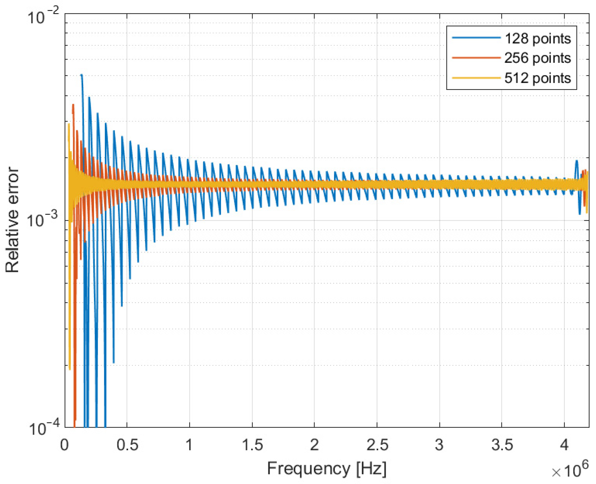
In a real acquisition, especially for interferometric measurements, it is impossible to get a perfect sine: in addition to the noise, frequency instability is always present. In the following simulations, the error induced in the IFFT by a signal with a non-constant frequency is calculated. The signal simulated is a sine wave subject to zero-mean frequency modulation, and the error is evaluated as the difference between the IFFT result and the original mean frequency.

Figure 5 shows the simulation results in the case of 0.3% of peak-to-peak frequency modulation. In this case, the gain in accuracy given by the increase in the number of points is decidedly lower with respect to a pure sine wave: 256 points and 512 points lead to approximately the same result. Similar results are also obtained with the addition of noise: Figure 6 shows the same simulations for SNR = 20 dB. Even in presence of noise, the accuracy improvement with the number of points is significantly lower than the pure single tone situation (Figure 3 and Figure 4).

The behavior of the estimation error depends on the shape of the frequency modulation, but the results obtained from a simulation campaign are still consistent with what is shown in Figure 5 and Figure 6. The main conclusion is that, in the case of a signal that does not have a perfectly stable frequency, as often happens in real applications, the estimate of the average frequency with IFFT techniques shows a limitation that is decidedly higher than what is expected for a pure single tone. These results will be able to explain the experimental measurements reported in Section 4.

4. Application to Absolute Distance Interferometry

The study of IFFT errors is now applied to a practical measurement case: an absolute distance meter based on self-mixing interferometry.

As described in [30], measuring the absolute distance to a target through a self-mixing interferometer requires modulation of the laser wavelength λ. The simplest technique to achieve this is to modulate the pump current I of the laser diode. If the wavelength variation is linear, i.e., with constant derivative over time ∂λ/∂t, an interferometric signal is obtained, with a frequency $f_{signal}$ proportional to the target distance. The measurement of the target distance s is given by [30]:

$$s=-\frac{{\lambda }^2}{2\cdot \left(\frac{\partial \lambda }{\partial I}\right)\cdot \left(\frac{\partial I}{\partial t}\right)}{f}_{signal}.$$

(2)

To linearize the wavelength variation, a pre-emphasis of the driving signal [38] is necessary, which must address both the frequency response of the modulation, mainly thermal, and the intrinsic non-linearity of the I-λ characteristic [39,40,41].

In order to cancel the contribution of the target movement, the distance measurement is obtained from the average between the measurements during ascendant and descendant phases of the modulation wave [30].

A self-mixing rangefinder was realized based on a VCSEL for working at distances up to about 20 cm. The main modulation frequency is about 9 kHz, and the signal is acquired at 8.4 MSPS by a microcontroller board that also generates the modulating waveform. The main modulation frequency was chosen as a good compromise between performances and measurement speed: at higher frequencies, the required distortion becomes too much, and the compensation is no longer optimal.

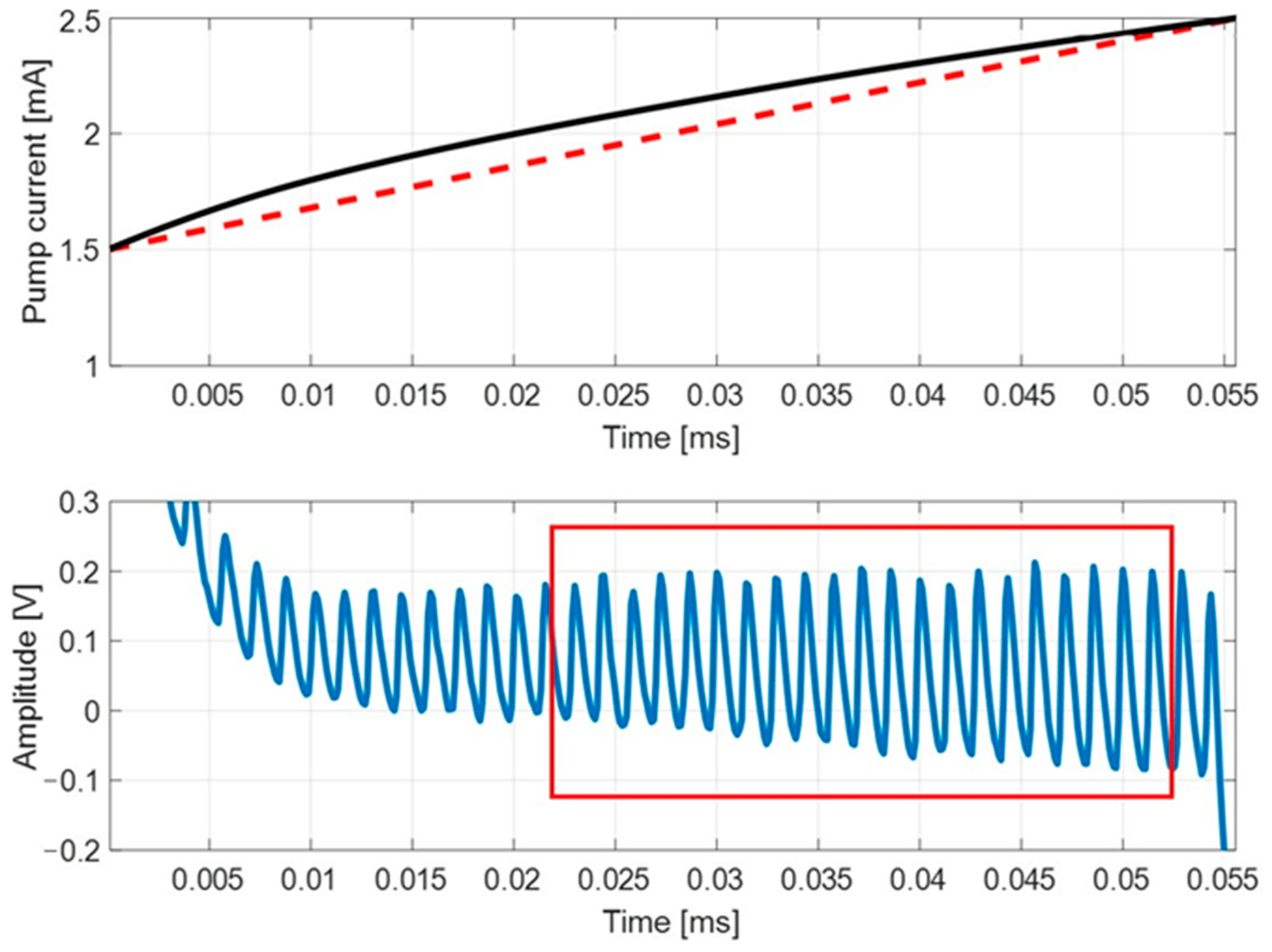
Figure 7 shows an example of a self-mixing signal, acquired in the case of target distance equal to 4.7 cm, where $f_{signal}$ is about 700 kHz. The current modulation (upper panel) is distorted in order to maximize the wavelength modulation linearity, estimated with the procedure described in [38] as better than 0.5% in the 256-points measurement interval, indicated by a box in Figure 7.

For characterizing the accuracy of the optical rangefinder, the target was mounted on a micrometric slide with 10 cm of travel. In order to avoid speckle effects, the target was realized by a single interface between air and glass, with 4% of reflection, and the laser beam was slightly divergent. In this way, it is possible to reach the wanted back-injection level (about C = 2), and the alignment procedure is quite easy [18].

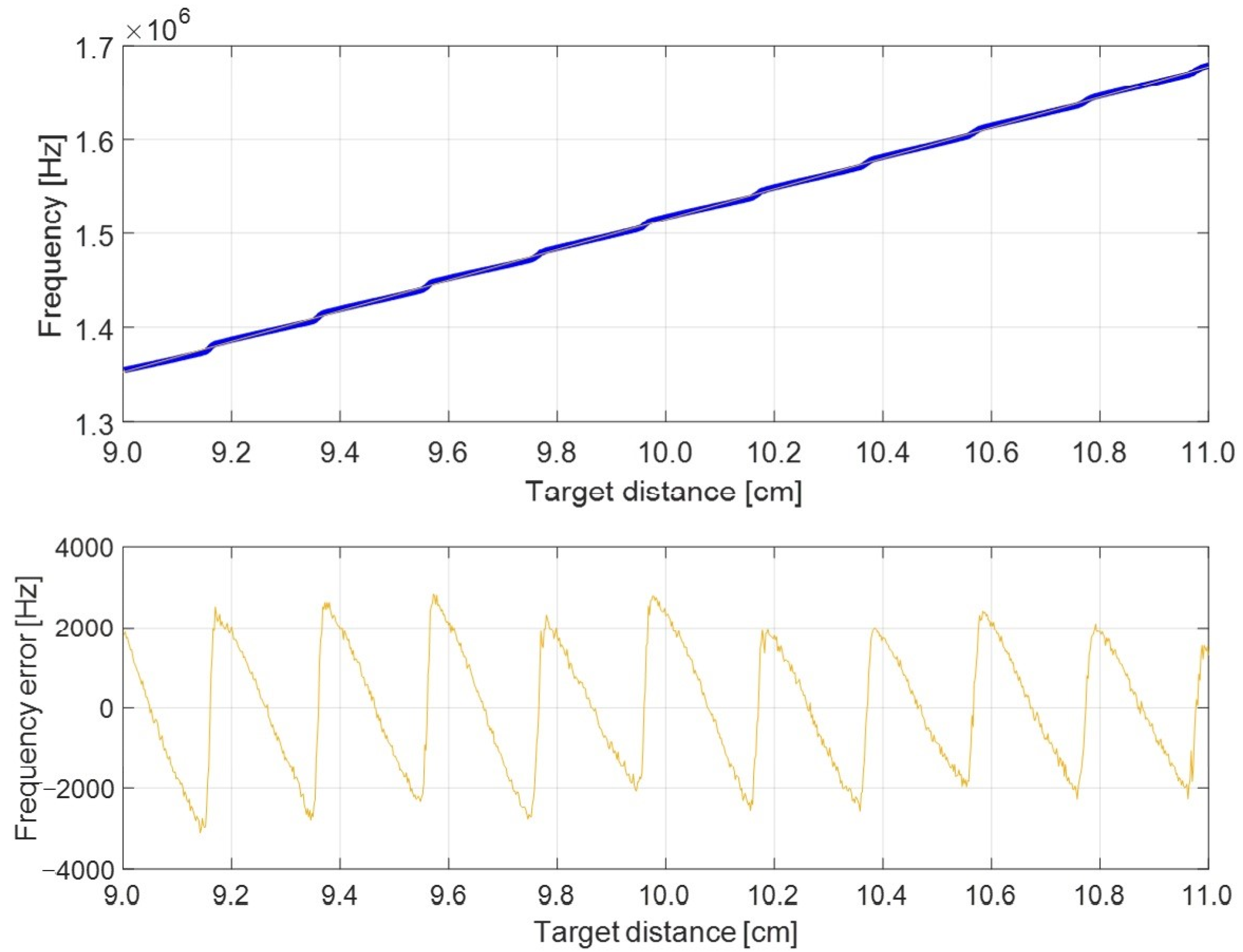
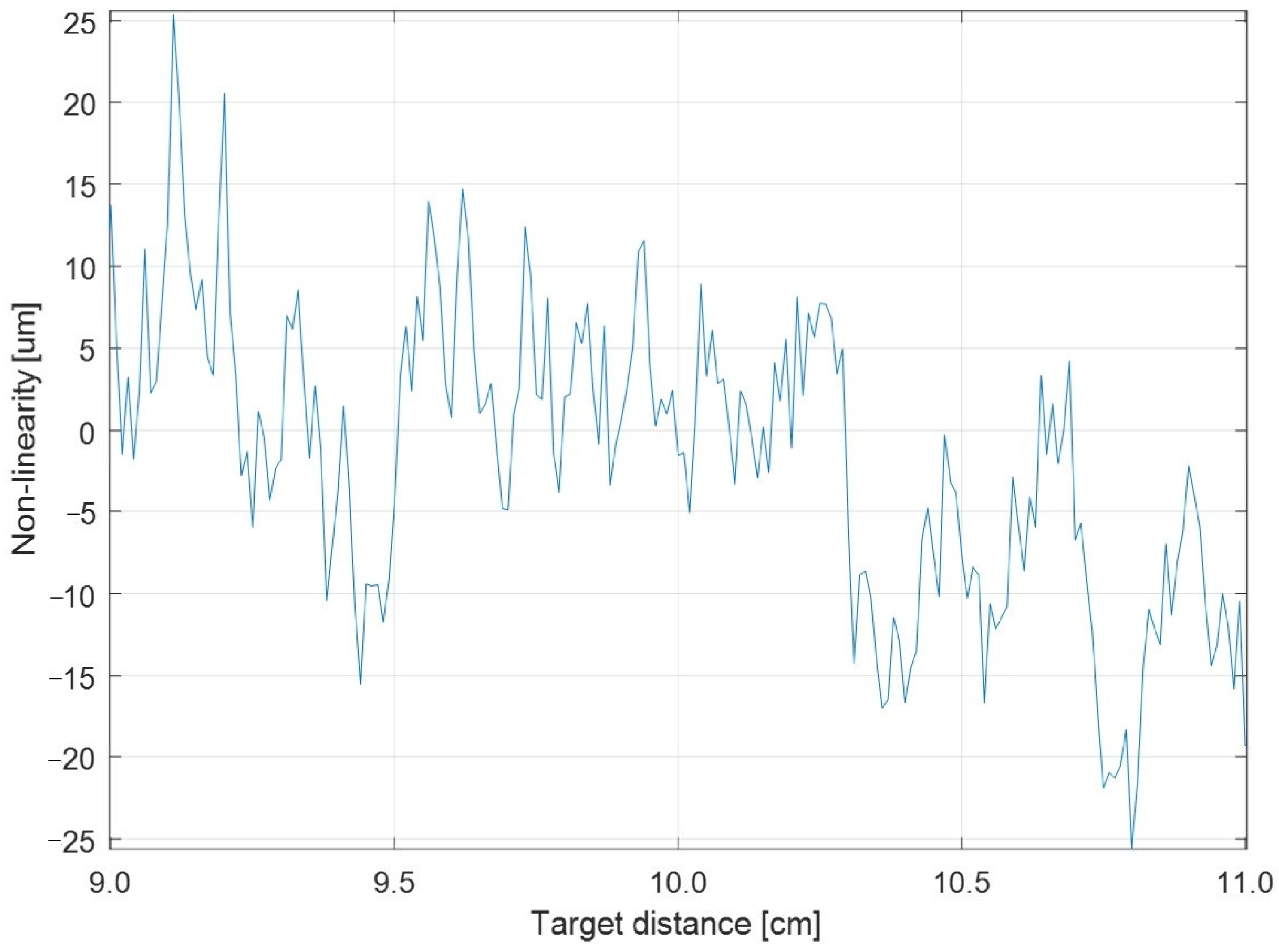
In the measurement campaign, 100 measurements were taken for each distance, with a step of 20 µm. For every measurement, the signal frequency was estimated using the IFFT. Figure 8 shows the estimated frequency, mean of 100 measurements, as a function of the target distance, and the non-linearity calculated as the difference between the measurement and a linear regression curve. The non-linearity, in this case, is mainly due to the deterministic error in IFFT frequency estimation. Indeed, its period is 32.8 kHz and coincides with 1 bin in the 256-point FFT at 8.4 MSPS. It is worth noting that without interpolation, the original FFT would have had errors of ±16.4 kHz; therefore, the IFFT improved the frequency resolution by about a factor of 8.

Figure 8 shows a relative peak error equal to about 1.3 × 10⁻³, one order of magnitude higher than the one expected from a 256-point IFFT (see Figure 3), but in good agreement with the simulations shown in Figure 5 and Figure 6. It indicates that the signal is not a pure sine wave: even after the linearization procedure, it still presents a small frequency modulation, estimated at about 0.3%. This error cannot be compensated from a practical point of view because it varies with temperature and is also influenced by the state of motion of the target. Even averaging procedures do not improve the results because, in the short term, the error is deterministic and cannot be canceled out by averaging. However, it can be noted that it generates an error that is always repeated in the same deterministic frequency positions. To get an improvement through averages, it is necessary to decorrelate the error contributions between one measurement and the next ones. The simplest way to decorrelate the measurements is to slightly vary the frequency of the modulation so as to obtain slightly different frequencies at the same target position. The method was already proposed in [38], but without evaluating the real improvement in the measurement.

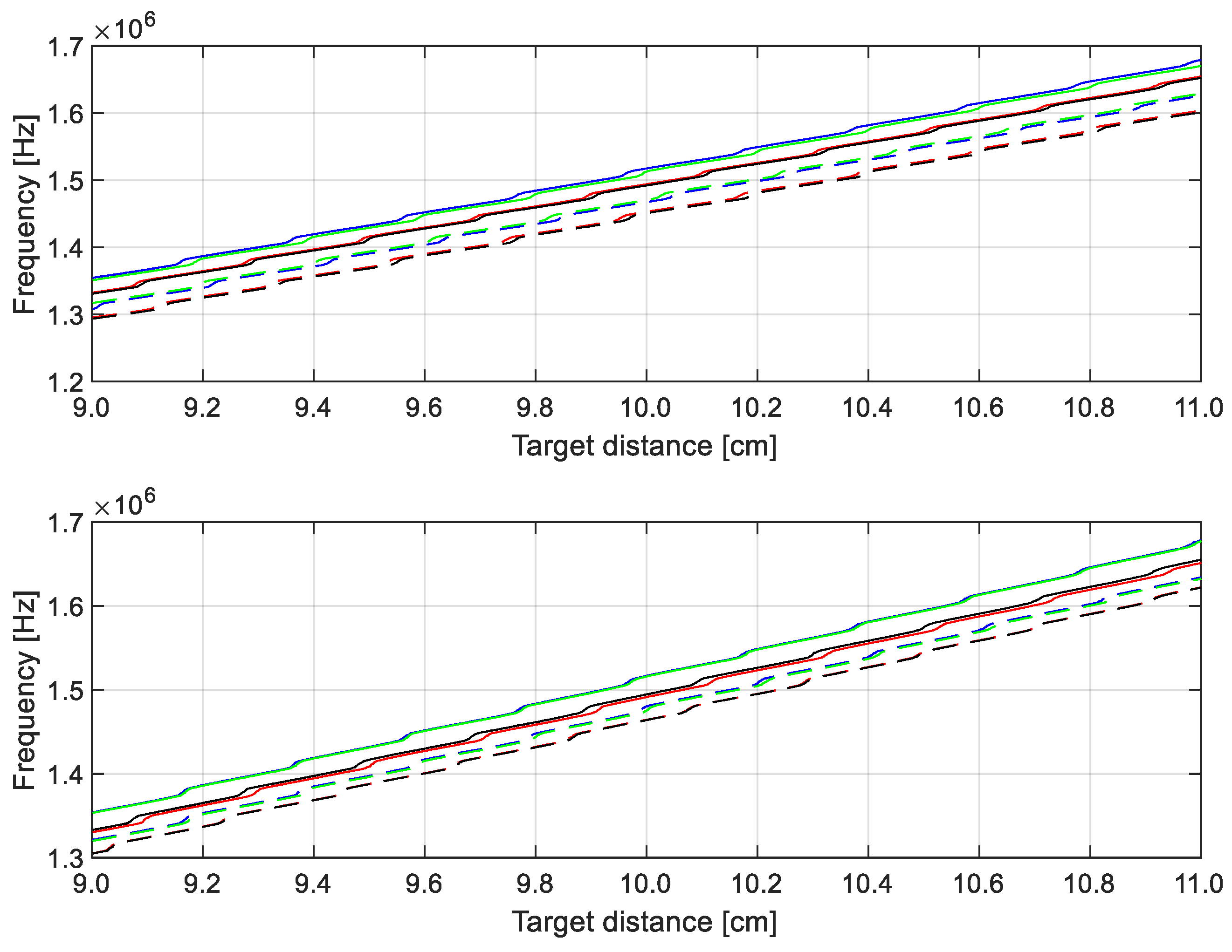
Next, Figure 9 and Figure 10 report the measurement results obtained with 8 modulation waves at frequencies varying linearly between 8.65 kHz and 9 kHz. The frequency values were chosen in order to optimize the positions of maximum error of the IFFT; considering a target distance around 10 cm, these positions are approximately equally distributed. The number of modulation waves is a choice dictated by a trade-off between accuracy and measurement speed. 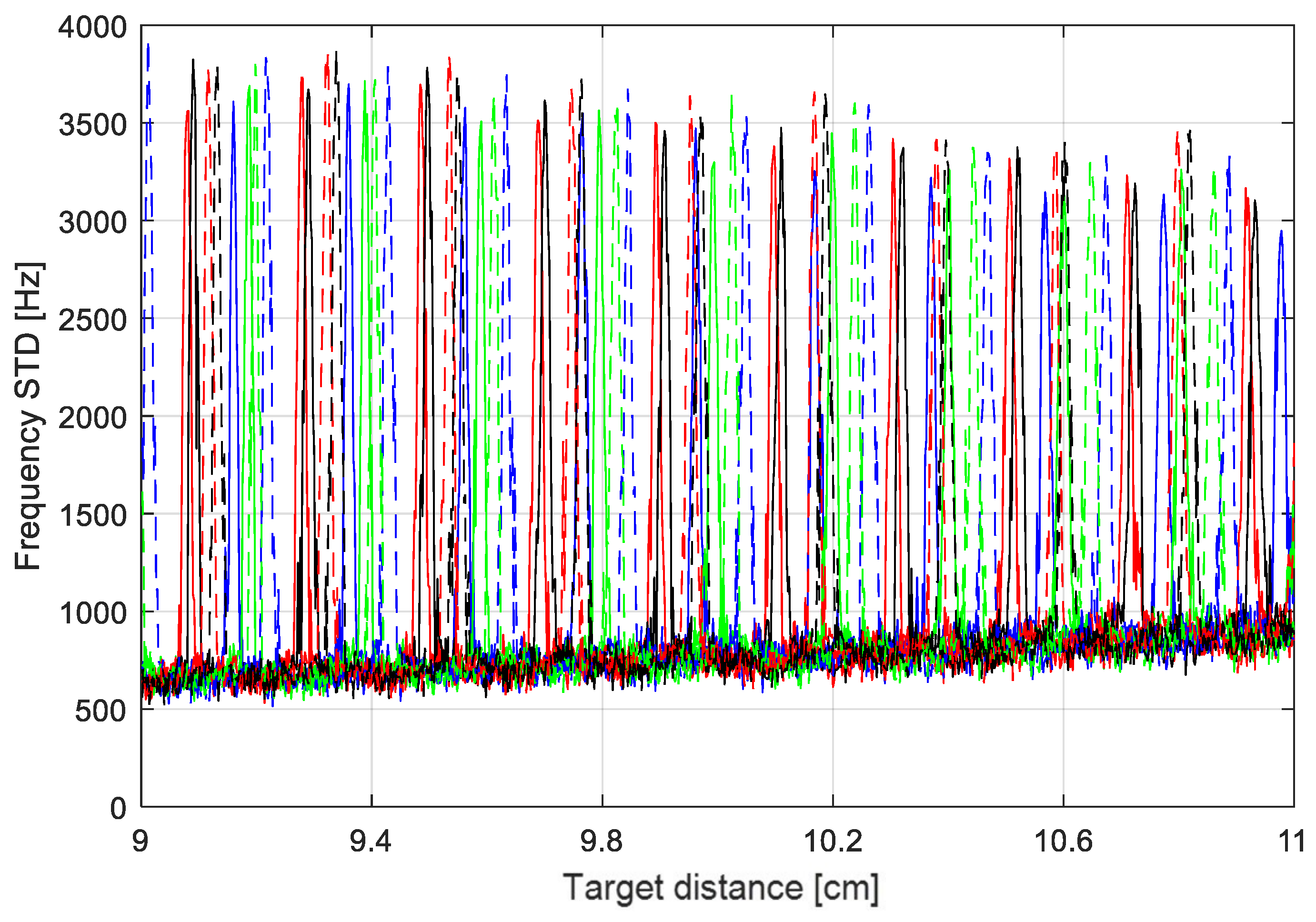Figure 9 shows the estimated frequencies for the 8 modulation waves, in ascending and descending phases, as a function of the target distance. The measurement step is 20 µm and every point is the average of 100 measurements. In order to better show how the choice of frequencies is optimized for the distance values considered, Figure 10 shows the standard deviations calculated over the 100 measurements carried out for each distance. Standard deviation is normally lower than 1 kHz, but it shows some peaks of more than 3 kHz. They happen at the critical points of the IFFT, when the two bins to the right and left of the FFT peak have a similar amplitude. In this situation, the IFFT adds a correction that can jump from the right to the left side of the main bin due to the noise, even with a very good SNR.

In Figure 10, it is evident that the choice of the 8 modulation frequencies corresponds to a good distribution of the critical points. For each considered distance, there is, at most, only one frequency in a critical position for the IFFT. This distribution optimizes the advantage of an averaging procedure, also allowing critical frequencies to be discarded.

Final results, given by the averages of the measurements of 16 IFFT (ascendant and descendant phases for 8 waves), are reported in Figure 11 as errors in the absolute distance measurement (difference between the slit position and distance estimated by the optical sensor). The final relative error is limited to about 10⁻⁴, one order of magnitude better than a measurement made on a single waveform. In comparison with previously reported self-mixing rangefinder, based on the same measurement principle, the improvement given by the proposed approach is evident. In [30], the achieved accuracy was about 100 µm, while in a more recent development [36], working at a lower modulation frequency (50 Hz instead of 9 kHz), which implies lower bandwidth, less noise and less distortion in modulation, after 50 averages, the absolute error was about 60 µm with the IFFT and 30 µm with an all-phase FFT.

5. Discussion

Through simulations, it was possible to explain the limits that occur experimentally in the use of the IFFT technique for distance measurement with self-mixing interferometers. The obtained results are of more general validity as, in numerous applications, the problem of estimating the frequency of a signal that is not a pure tone is encountered. The proposed method of improving the estimation accuracy in these cases consists of implementing a series of uncorrelated measures, from which to obtain an average. For the specific application of the self-mixing rangefinder, the proposed technique is achieved through multiple modulations at slightly different frequencies.

In the creation of instruments, there is always a tradeoff between accuracy and measurement speed. In this specific case, it is demonstrated that it is more efficient to carry out an IFFT on fewer points (256) by increasing the number of averages, rather than increasing the points of the IFFT (512 or 1024). The reasons are multiple: the 256-point IFFT can also be calculated faster by a microcontroller; at the same sampling rate (8.4 MSPS in this case), a lower number of samples allows for higher modulation frequency, with the benefit of a lower contribution from any movement of the target; at the same final measurement rate, there is the possibility of making more averages and, therefore, reducing the systematic errors of the IFFT. For example, the realized prototype of the self-mixing rangefinder with 8 modulating waveforms allows for 1000 measurement per second. It was the best compromise between speed and accuracy experimentally found.

The advantages of the proposed technique are evident from the measurement results, achieving an order of magnitude improvement in deterministic errors compared to a single modulation. Even compared to the results already published in the literature, a clear improvement is noted, such as in comparison with [36]. The main limit of the proposed approach is the need for a longer measurement time. In the specific example, the realized sensor works at 1000 measurements per second, while with a single modulation, it could, in theory, work at 9000 measurements per second.

6. Conclusions

The theoretical performances of the IFFT, known from the literature [23], are often not found in the practical applications of real signals. An emblematic case is that of interferometric distance measurements, where the assumption of having a pure sinusoidal signal is not verified in practice. The distance information is contained in the average measured frequency, but the classical frequency estimation techniques provide deterministic errors on the measured value, which cannot be improved by simple averaging operations. The first part of the work consisted of demonstrating, through simulations, that the performances obtained in real prototypes are compatible with the presumed non-idealities of the measured interferometric signal, mainly the residual frequency modulation. The next proposal of this work consisted of decorrelating the individual errors by moving the frequency to be measured between one measurement and the next. In the specific case of the optical rangefinder, this shift was achieved through multiple modulations at slightly different frequencies. The experimental results confirmed an improvement of about one order of magnitude in the measurement accuracy, with 8 modulation waveforms.

The results of this study, aimed at optimizing the performance of the optical rangefinder, can be extended to various applications where the real-time estimation of the average frequency of a signal is required.