MOHVAE-B: A Hierarchical Variational Autoencoder–Bayesian Network Framework for Multi-Omics Integration and Glioma Biomarker Discovery

Abstract

Gliomas represent the most prevalent type of brain tumor, with their most aggressive variant, glioblastoma multiforme, associated with high mortality rates. Due to their elevated molecular heterogeneity, accurate classification of gliomas has presented significant challenges. Therefore, considerable effort has been dedicated to identifying relevant biomarkers that improve early diagnosis and unveil new areas for treatment. Advances in high-throughput sequencing technology have enabled public resources such as The Cancer Genome Atlas (TCGA) to provide large-scale data from various cancers, allowing researchers to perform more comprehensive analysis of this disease. In this study, we introduce MOHVAE-B, a comprehensive framework designed for the integration of multi-omics data and biomarker discovery using data from TCGA. MOHVAE-B employs a supervised hierarchical variational autoencoder integrated with SHAP-based interpretability to effectively integrate high-dimensional multi-omics data and extract the most influential features driving the model’s predictions. Subsequently, Bayesian Networks (BNs) are constructed to model conditional dependencies between the selected features, providing insights into their possible relations. Applied to the TCGA glioma cohorts, MOHVAE-B achieved a near-perfect AUC of $0.9993$ and successfully identified high-impact features related to glioma classification. For glioblastoma multiforme, this included six novel candidates: LINC02172, NACA2, LINC01114, HNRNPA1P48, PPIAL4G, and LINC01558. For low-grade gliomas, the model highlighted AMER2 as a promising marker. Across both cohorts, PMP2 stood out as a particularly strong candidate for a potential role in glioma pathogenesis. The constructed BNs provided an additional layer of validation, reinforcing NACA2 as a candidate of interest in glioma biology.

1. Introduction

Gliomas are a type of brain tumor that comprise 80 percent of all malignant brain tumors [1]. Glioblastoma multiforme, the most common and aggressive type of glioma, is associated with a poor median survival of 8 months for adults [2]. Due to the low patient survival, substantial effort has been made to improve the early diagnosis of this disease. One of the main focuses remains on accurately classifying the type of glioma. This task has proven challenging due to the large genetic and molecular heterogeneity of these tumors. To this end, the World Health Organization Classification of Tumors of the Central Nervous System, which initially classified tumors according to their morphological and histopathological traits, has started to incorporate additional molecular markers to refine the diagnostic accuracy [3]. Simultaneously, researchers have dedicated considerable effort to identifying new relevant biomarkers associated with this disease.

Advancements in high-throughput genomic technologies have facilitated the collection of an increasing amount of biological data. This progress has resulted in large-scale public datasets, such as The Cancer Genome Atlas (TCGA) [4], becoming invaluable resources for researchers aiming to deepen their understanding of these diseases. These datasets offer an extensive array of data composed of various omics modalities (e.g., genomics, epigenomics, transcriptomics), enabling a more comprehensive exploration of the biology underlying cancer diseases. Specifically concerning gliomas, TCGA provides two primary collections: TCGA-GBM, which focuses on glioblastoma multiforme, and TCGA-LGG, which includes low-grade gliomas. Integrating these diverse types of omics data presents a unique opportunity to uncover novel biomarkers and examine tumor heterogeneity in greater detail.

However, the high-dimensional characteristics of multi-omics data pose significant challenges for their analysis. Due to the extensive number of features involved, the analysis of multi-omics data frequently requires substantial computational resources and is particularly susceptible to overfitting. This situation emphasizes the necessity of transforming the data into more manageable subsets that are more suitable for biological interpretation. For this purpose, deep learning methodologies have been increasingly explored in recent years. Among the most promising models are Variational Autoencoders (VAE) [5], which have demonstrated promising results in tasks such as feature extraction and effective dimensionality reduction. While considerable research has been directed toward VAEs, most applications of these models predominantly focus on using multi-omics data for tasks such as pan-cancer classification, tumor subtyping, and survival analysis. Few investigations have examined the application of VAEs for the discovery of novel biomarkers, and those that have, recognized inherent limitations in their methodologies [6]. This gap highlights an opportunity for creating frameworks that prioritize interpretability alongside the powerful capabilities of VAEs. In this context, probabilistic graphical models, particularly Bayesian Networks [7], enable reasoning about complex dependencies among variables and provide interpretable structures that can support biological insight.

In this study, we aim to identify novel biomarkers associated with gliomas. To achieve this, we propose MOHVAE-B, a Multi-Omics Hierarchical Variational Autoencoder– Bayesian Network framework designed specifically for comprehensive biomarker discovery. MOHVAE-B utilizes H-VAE to effectively learn the latent representations associated with each cancer cohort from TCGA. At the same time, SHapley Additive exPlanations (SHAP) values are integrated into the H-VAE model, providing a way to extract the most significant features associated with each cancer type. The selected features will then undergo biological interpretation with the help of Bayesian Networks (BNs), which will model conditional dependencies between them and provide a probabilistic perspective on their potential biological interactions.

2. Related Work

The domain of “omics” refers to the investigation of extensive data produced through high-throughput technologies, encompassing disciplines such as transcriptomics, proteomics, and epigenomics. Each branch of omics offers unique insights into specific molecular layers of biological processes. Given that single-omics studies are limited in their ability to represent the intricate complexity of biological systems [8], researchers are increasingly adopting multi-omics methodologies to achieve a more comprehensive understanding. Nevertheless, multi-omics methodologies encounter numerous challenges, notably, the high dimensionality of the data introduces significant computational challenges in terms of integration [9].

Over recent years, VAEs have emerged as powerful tools for various tasks, including generative modeling, dimensionality reduction, and clustering. Advancements in their architectures have significantly improved their capability to integrate and model heterogeneous data, particularly in the domain of multi-omics integration. One of the first studies to inspire further exploration in this area was conducted by Zhang et al. [10], who proposed OmiVAE, a VAE that integrated a task loss into the VAE’s overall loss for pan-cancer classification. Withnell et al. [11] extended this model into XOmiVAE, a variation that facilitates the interpretability of the previous model by leveraging SHAP values [12], revealing gene contributions to subsequent tasks.

Franco et al. [13] compared four variations of AEs—vanilla, denoising, sparse, and variational—across tasks such as tumor subtype classification and survival analysis. Similarly, Simidjievski et al. [14] explored multiple VAE variants, including CNC-VAE, X-VAE, H-VAE, and MM-VAE, identifying superior performance for H-VAE and CNC-VAE. Their work also demonstrated that replacing the KL divergence with MMD improved performance.

Concurrently, BNs have gained significant popularity over the last decade, particularly in the context of multi-omics research. They have been extensively applied to TCGA data for biomarker discovery and clustering analysis. Kuipers et al. [15] developed a BN model across 22 TCGA cancer types, identifying novel patient clusters that improved survival prediction. Bu et al. [16] applied BNs to lung cancer data, pinpointing two key genes involved in disease progression, while Zhang et al. [17] modeled causal gene relationships in ovarian cancer, identifying previously unreported genes influencing patient survival.

3. Materials and Methods

3.1. Data Extraction

For this study, we retrieved TCGA datasets via the UCSC Xena platform [18]. From each available TCGA cancer cohort, we downloaded DNA methylation, gene expression, protein expression, and clinical data. In total, we considered 32 different types of cancer, excluding Acute Myeloid Leukemia since there was no protein expression data provided for this type of cancer. The DNA methylation data is represented by $\beta$-values ranging between 0 (unmethylated) and 1 (fully methylated), quantifying methylation levels at CpG sites. Gene expression data were obtained in Transcripts per Million (TPM), transformed as ${log}_2(TPM+1)$. The TPM metric was selected for its normalization for both gene length and sequencing depth. Protein expression data were generated by Reverse Phase Protein Array analysis. Lastly, clinical patient metadata, including vital status, survival time, sample type, and other pathological characteristics, were also downloaded.

3.2. Data Preprocessing

Data preprocessing procedures were applied to ensure data consistency across omics layers. For DNA methylation, we used the human reference genome (hg38) annotation to remove probes located on sex or mitochondrial chromosomes, non-CpG probes, SNP-associated probes, and those not mapping to protein-coding, lncRNA, or miRNA genes (99,738 removed). For gene expression data, we removed Ensembl IDs associated with sex or mitochondrial chromosomes, and retained only the features mapping to the same gene categories as DNA methylation (36,074 removed). For protein expression data, we removed features with validation status other than “Valid” and those associated with previously removed Ensembl IDs (211 removed). A summary of the preprocessing steps and the number of removed features for each omics layer is provided in

Table 1. Number of features before and after independent filtering for each omics layer.

Data Type	Features
	Initial	Final
DNA Methylation	486,426	386,688
Gene Expression	60,659	24,585
Protein Expression	486	275

.

Following independent filtering of each omics layer, we intersected samples across all three modalities to meet the multi-omics integration requirement of complete data across all layers. This process reduced the sample count from 9598 (DNA Methylation), 11,085 (Gene Expression), and 7904 (Protein Expression) to 6342 shared samples. Afterwards, only TCGA sample type codes 01 (Primary Solid Tumor) and 11 (Solid Tissue Normal) were retained. Samples with codes 02 (Recurrent Solid Tumor), 05 (Additional New Primary), and 06 (Metastatic Tumor) were excluded because treatment exposure, multiple primary contributions from the same patient, or metastatic adaptation could alter the original molecular profile. This filtering step removed 319 additional samples, yielding a final cohort of 6023 samples across 32 cancer types, of which 6002 are primary solid tumor samples and 21 are solid normal tissue samples (included in the TCGA-BRCA cohort, where matched normal tissue is available). The counts per cohort at each stage of the preprocessing pipeline are shown in

Table 2. Number of samples per cohort at each stage of the preprocessing pipeline: per-modality counts before intersection, after three-way intersection, and after sample-type filtering.

Cohort	DNA Methylation	Gene Expression	Protein Expression	After Intersection	After Filtering
TCGA-ACC	80	79	46	46	46
TCGA-BLCA	437	428	343	338	338
TCGA-BRCA	893	1226	919	655	630
TCGA-CESC	312	309	172	170	170
TCGA-CHOL	45	44	30	29	29
TCGA-COAD	346	514	363	249	247
TCGA-DLBC	48	48	33	33	33
TCGA-ESCA	202	198	126	125	125
TCGA-GBM	155	175	243	44	33
TCGA-HNSC	580	566	354	347	347
TCGA-KICH	66	91	63	63	63
TCGA-KIRC	483	610	478	290	290
TCGA-KIRP	321	323	216	213	212
TCGA-LGG	534	534	435	435	429
TCGA-LIHC	430	424	184	181	181
TCGA-LUAD	503	589	365	319	319
TCGA-LUSC	412	552	328	256	256
TCGA-MESO	87	87	62	62	62
TCGA-OV	10	429	432	9	9
TCGA-PAAD	195	183	120	113	113
TCGA-PCPG	187	187	82	82	79
TCGA-PRAD	553	554	352	351	351
TCGA-READ	106	177	132	78	77
TCGA-SARC	269	265	226	223	220
TCGA-SKCM	475	473	352	350	89
TCGA-STAD	397	448	357	296	296
TCGA-TGCT	156	156	122	122	118
TCGA-THCA	571	572	379	377	375
TCGA-THYM	126	122	90	87	87
TCGA-UCEC	482	585	440	339	339
TCGA-UCS	57	57	48	48	48
TCGA-UVM	80	80	12	12	12
Total	9598	11,085	7904	6342	6023

. All cohorts were aggregated within each omics layer, producing three unified datasets, one per omics modality.

Gene expression and protein expression were rescaled to the $[0,1]$ interval using min-max normalization, both to satisfy model requirements and to make their ranges comparable to DNA methylation $\beta$-values. For DNA methylation data, features with variance below 5% were removed. For both DNA methylation and gene expression data, features with more than 5% missing values were discarded. No additional filtering was applied to protein expression data due to the small number of available features. Remaining missing values were subsequently imputed using median imputation, whereby each missing entry was replaced by the median of the corresponding feature across all samples. The final datasets contained 29,685, 24,074, and 275 features for DNA methylation, gene expression, and protein expression, respectively, totaling 6044 samples. The final feature counts are reported in

Table 3. Final number of features after variance and missing-value filtering.

Data Type	Features
	Initial	Final
DNA Methylation	386,688	29,685
Gene Expression	24,585	24,074
Protein Expression	275	275

.

3.3. Hierarchical Variation Autoencoder Model

To identify biomarkers relevant to gliomas, we adapted and built upon a H-VAE model based on the supervised mixed integration architecture proposed by Benkirane et al. [19]. The proposed H-VAE architecture was designed to integrate multi-omics data in a supervised fashion. The model operates through a two-phase training process.

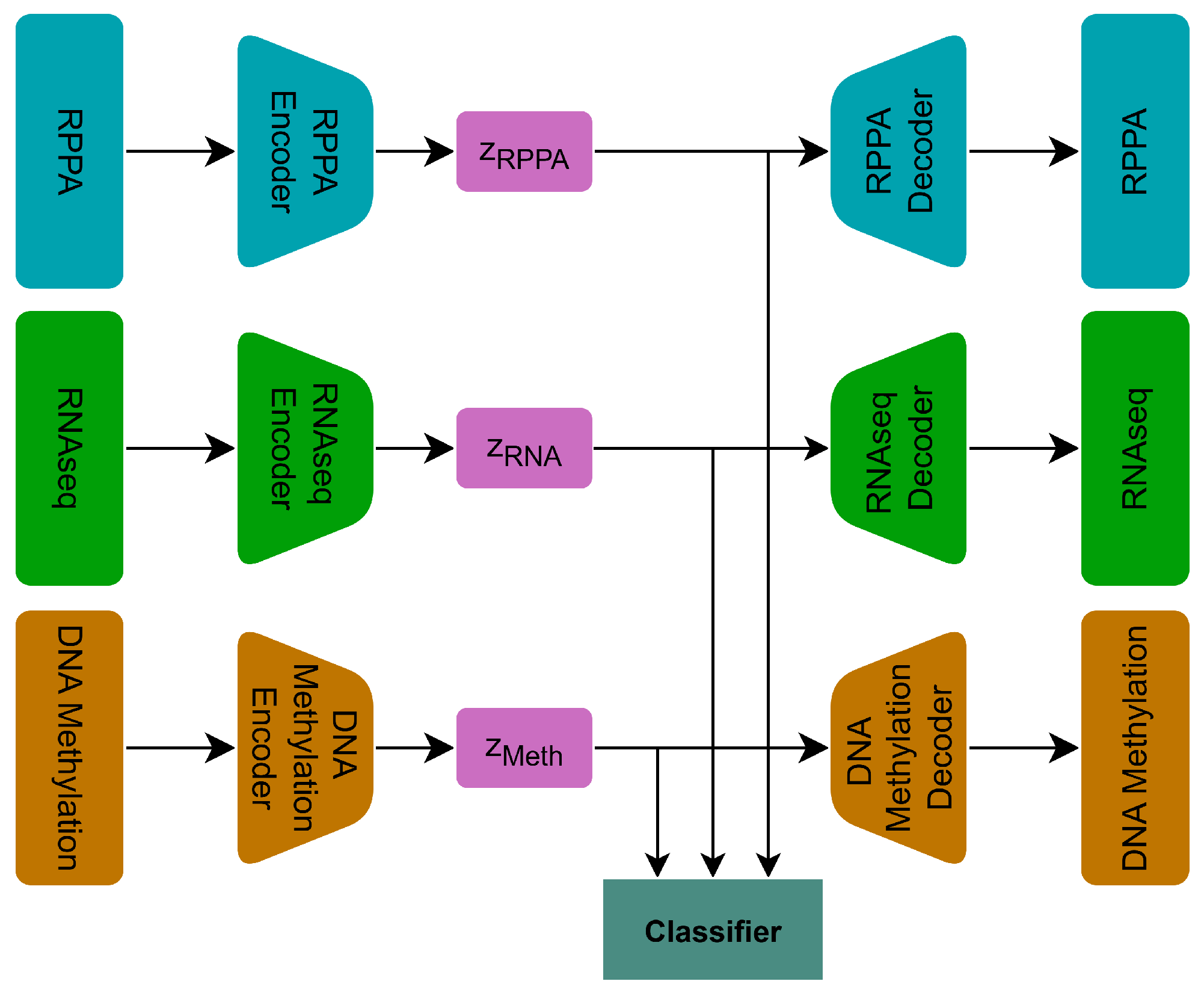
The first phase is shown in Figure 1. Each omics modality is associated with an independent autoencoder (AE). Each encoder generates a latent representation that is used both to reconstruct the original input and to classify the sample type via a dedicated classifier network. The training loss for this phase is computed as the sum of the reconstruction and classification losses for each autoencoder.

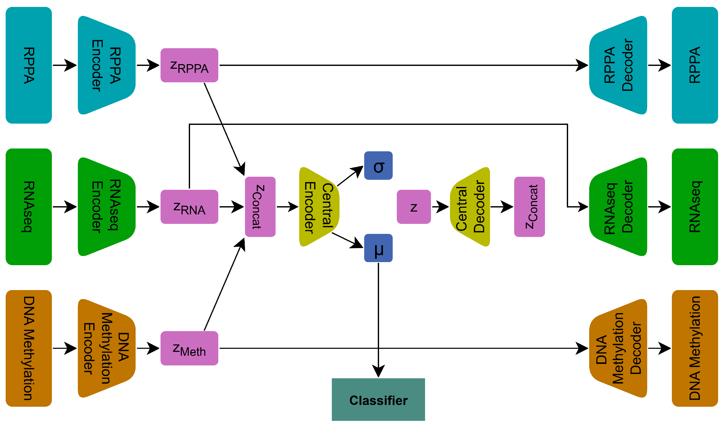
In the second phase, illustrated in Figure 2, the per-source encoders continue to refine their subrepresentations as in the first phase. However, in this phase, the classification loss is computed from a latent representation produced by a central VAE, rather than from each omics-specific latent representation independently. Specifically, each omics-specific latent space is concatenated and passed into a central VAE. This step aims to capture the relationships between the different omics layers. The central encoder outputs mean $\mu$ and $\sigma$ vectors, which define the central latent space z. The latent vector z is passed to the central decoder for reconstruction. Simultaneously, the $\mu$ vector serves as input to the classifier network, where, analogous to phase 1, the classification loss is calculated.

The classifier network consists of a three-layer fully connected feed-forward neural network, where the final layer utilizes a softmax activation over 33 output classes corresponding to the number of sample types considered in this study.

The model was trained by optimizing a composite loss function tailored to each phase of the training process. The reconstruction loss for all AEs and the central VAE is formulated as follows:

$$\begin{array}{c}\hfill L_{autoencoder/VAE}=MSE(x,\widehat{x})={\displaystyle \frac{1}{N}}{\displaystyle \sum _{i=1}^N}{(x_i-{\widehat{x}}_i)}^2,\end{array}$$

where x represents the input, $\widehat{x}$ the output from the decoder and N the number of features associated with each input dataset. For the central VAE introduced in phase 2, a regularization term is used to enforce a structured latent space. Following recent studies [14], we chose to use the maximum mean discrepancy (MMD) loss. Let p and q represent two distributions; the MMD distance is formulated as:

$$\begin{array}{c}\hfill \mathrm{MMD}(p\left(x\right)\parallel q\left(x\right))={\mathbb{E}}_{p\left(x\right),p\left(x^{\prime }\right)}\left[k(x,x^{\prime })\right]+{\mathbb{E}}_{q\left(x\right),q\left(x^{\prime }\right)}\left[k(x,x^{\prime })\right]-2{\mathbb{E}}_{p\left(x\right),q\left(x^{\prime }\right)}\left[k(x,x^{\prime })\right],\end{array}$$

where $k(x,x^{\prime })$ is a kernel function, and x and $x^{\prime }$ are two sample points. The kernel was specified as Gaussian, such that: $k(x,x^{\prime })=exp\left(-{\displaystyle \frac{\parallel x-x^{\prime }{\parallel }^2}{2{\sigma }^2}}\right)$. To guide the model towards accurately discriminating different cancer samples, following studies such as [11], a classification loss component was also integrated into the total loss of our model. This loss was defined as a categorical-entropy loss given by the equation:

$$L_{class}=\sum _i{y}_{i}log\left({\widehat{y}}_i\right),$$

(1)

where $y_i$ is the ground truth for the $i^{th}$ sample, and  ${\widehat{y}}_i$ represents the model’s estimation. The total loss for each phase of the model is represented as a weighted sum of its components. Let “omics” denote the set of all omics modalities used in the model. For phase 1, we have:

$$L_{total}^{\left(Phase1\right)}=\sum _{\mathrm{omics}}\left(L_{autoencoder}^{\left(omics\right)}+\alpha L_{class}^{\left(omics\right)}\right),$$

(2)

and for phase 2:

$$\begin{array}{c}\hfill L_{total}^{\left(Phase2\right)}=\sum _{\mathrm{omics}}{L}_{autoencoder}^{\left(omics\right)}+L_{VAE}+\beta L_{MMD}+\alpha L_{class},\end{array}$$

where $\beta$ and $\alpha$ control the contributions of the regularization and classification losses, respectively.

The H-VAE architecture was implemented using the PyTorch deep-learning library (version 2.0.1). The network utilizes fully connected blocks, where each block consists of a linear layer followed by batch normalization and/or dropout regularization, and an activation function. Batch normalization was used to address internal covariate shift problems [20]. Dropout regularization was applied to mitigate overfitting. Regarding the activation function, we chose the LeakyReLU because it addresses the “dying ReLU” problem, ensuring consistent gradient flow throughout our model. The model’s weights were initialized using the Kaiming (He) uniform method [21], which is recommended for networks using ReLU (and related) activations. All biases were initialized to zero. Exceptionally, sigmoid activation was applied to the AEs decoders’ final layers, ensuring the model’s output matches the normalized input domain $[0,1]$.

To identify the optimal model configuration given our data, we utilized the Optuna hyperparameter optimization framework [22]. The objective was set to maximize the ROC-AUC score on the test sets, emphasizing the model’s discriminative performance. A two-stage strategy was used: the first stage tuned training parameters (e.g., dropout, learning rate, regularization), while the second optimized architectural dimensions (encoder, decoder, and classifier layers) based on the best settings from stage one.

Regarding model training and evaluation, we employed a repeated stratified 5-fold cross-validation scheme. In each repetition, the dataset was divided into five stratified folds, preserving the proportion of samples from each class. Within each fold, one split (20% of the data) was used as the test set, while the remaining 80% of the data were further split into training (60% of the total dataset) and validation (20% of the total dataset) sets. The 5-fold procedure was repeated four times, resulting in a total of 20 independent model runs. Despite the powerful explainability of SHAP, the ranking of feature importance can be sensitive to the specific dataset used for training. The repeated cross-validation scheme was therefore implemented to mitigate variability across splits, ensuring that only the most robust features, which are consistently ranked highly across different runs, are chosen.

The Adam optimizer was used during training. All models were trained on an NVIDIA GeForce GTX 1650 GPU with 4 GB of VRAM.

3.4. Model Interpretability with SHAP

A primary goal of this study is not only to classify cancer subtypes correctly but also to identify the features that drive the model’s predictions, particularly those that contribute most to a sample being classified as a glioma. To this end, we used SHAP values to interpret the predictions obtained by our H-VAE model, leveraging the DeepExplainer class from the shap python library, which is tailored for deep neural networks. SHAP values were computed on a subset of tumor and background samples. While the tumor subset is composed of samples from the target cancer, the background subset consists of samples randomly drawn from all other non-target cancer classes in the dataset. This allows the model to evaluate the impact of the target class features against a comprehensive pan-cancer baseline.

Due to the limited number of available samples in the TCGA-GBM cohort, which totaled only 33 samples, the subset size was set to $n=30$ to maximize the stability of SHAP value estimation while still allowing for a slight degree of sample-set variability across the 20 model runs. In contrast, for the TCGA-LGG cohort, a subset of $n=200$ was selected, balancing computational efficiency with statistical robustness. Feature importance values were then derived as the mean absolute SHAP scores across tumor samples.

For each of the 20 model runs, we extracted the top 50 most important features for each combination of omics modality (DNA methylation and gene expression) and glioma subtype (GBM and LGG). The final feature set for each modality-cancer combination was determined by selecting the features with the highest frequency of appearance across all 20 runs.

3.5. Biological Validation of Top Features Extracted

3.5.1. Literature Search

A systematic literature search was conducted for each top feature identified by our H-VAE model using the PubMed database. For each gene X, we performed three Boolean search queries:

• “X” AND “glioma”—has gene X been linked to glioma?
• “X” AND “cancer”—has gene X been linked to any kind of cancer?
• “X” AND “glioma” AND (“2020”[Date - Publication]:(“2025”[Date - Publication]) —has gene X been linked to glioma in the last five years (2020–2025)?

3.5.2. Differential Expression Analysis

To contextualize the biological relevance of the top features identified by the H-VAE model, we performed a differential expression analysis (DEA) for the top genes selected for each glioma subtype. Using GENCODE v23 annotation files, we mapped every Ensembl ID and every CpG probe ID to their corresponding gene symbol(s). Because the TCGA-LGG dataset contains no normal samples and the TCGA-GBM dataset contains too few for a robust comparison, GTEx brain tissue was used as the normal reference [23]. This introduces perfect confounding between biological condition and data source, as the tumor samples come only from TCGA and the normal samples come only from GTEx. To mitigate this, gene expression data were obtained from the UCSC Xena TOIL recompute dataset [24], which reprocesses TCGA and GTEx RNA-seq samples through a shared pipeline, thereby reducing batch effects that arise when independently processed datasets are compared. From the UCSC Xena TOIL recompute dataset, TCGA primary tumor samples, 153 for GBM and 509 for LGG, were compared with 258 GTEx normal samples drawn from five brain regions: frontal cortex, cortex, anterior cingulate cortex, hippocampus, and amygdala. Values for the gene expression data are provided as ${log}_2(\mathrm{expected}\mathrm{count}+1)$.

Low-expressed genes were removed by requiring a ${log}_2(\mathrm{expected}\mathrm{count}+1)$ value greater than 1 in at least $20\%$ of samples in either the tumor or the normal group. To address the batch effects possibility, a principal component analysis (PCA)-based quality-control step was then applied: samples lying more than three standard deviations from the mean on either PC1 or PC2 were flagged as outliers and excluded to reduce the influence of potential technical artifacts on downstream analysis.

Differential expression was assessed with the limma R package (version 3.64.3). Linear modeling with empirical Bayes moderation (eBayes with trend = TRUE) was applied to stabilize variance estimates across genes. A gene was considered differentially expressed if it satisfied both an $\text{FDR-adjusted}p\text{-value}<0.05$ and an absolute ${log}_2$$\mathrm{fold}\mathrm{change}>1$.

3.5.3. DNA Methylation Characterization

As the final step of validation, to be able to generate informed interpretations regarding the biological relevance of the top DNA methylation features, we linked each probe to its associated gene(s), CpG island status, and distance to the transcription start site (TSS). Combining Illumina’s standard with the available data provided in the annotation file (distToTSS), we categorized probes based on their distance to the nearest TSS as: TSS200 (−200 base pairs (bp) to 0 bp), TSS1500 (−1500 bp to −200 bp), or gene body (downstream of the TSS, >0 bp). Afterward, we computed the mean $\beta$-values across tumor and normal samples separately for GBM and LGG, and derived the methylation difference ($\Delta \beta$) for each probe.

To establish an accurate baseline for this comparison, normal control samples were sourced from the Gene Expression Omnibus (GEO) dataset GSE66351 [25], which provides Illumina HumanMethylation450 profiles from 16 healthy frontal cortex samples subjected to Fluorescence-Activated Nuclear Sorting (FANS), a process that separates neuronal (NeuN+) from glial (NeuN−) nuclei. By selecting the NeuN− fraction as the normal reference, both tumor and control samples are predominantly composed of glial cells, thereby reducing confounding methylation differences arising from cell-type composition. Although the number of normal samples is limited, this dataset was deliberately chosen for its cell-type specificity.

Due to the study design, the dataset exhibits perfect confounding between disease status and data source, as tumor samples originate exclusively from TCGA and normal samples exclusively from GEO. Consequently, standard batch-correction algorithms such as ComBat cannot be applied, as they require overlapping cconditions across batches. However, given that both cohorts were profiled on the same Illumina HumanMethylation450 platform, eliminating probe-design differences, and that the cell-type composition of the normal samples matches that expected in TCGA glioma samples, the impact of residual technical variation is substantially reduced. Moreover, our interpretation is restricted to probes exhibiting substantial methylation differences, $|\Delta \beta |>0.2$, a threshold at which biological signal is expected to dominate over technical variation.

3.6. Bayesian Network

To infer dependencies among the top features identified by the H-VAE model for each omics modality (in particular, DNA methylation and gene expression), BNs were constructed as a complementary interpretability component. Because BNs are constructed independently for each omics modality, the sample intersection constraint required by the multi-omics integration model does not apply. Given this, we used all available TCGA samples available for each cohort, rather than restricting to the intersected cohort as done during the H-VAE training. For each cohort, we removed all non primary solid tumor samples as well as all duplicate patients. In the final dataset, gene expression data comprised 673 samples, 157 GBM and 516 LGG, while DNA methylation data comprised 657 samples, 141 GBM and 516 LGG.

The networks were implemented using pgmpy’s library functions, which require discrete input data. Prior to discretization, features with insufficient variability were removed. The remaining continuous features were then discretized into four bins labeled as “very low”, “low”, “medium”, or “high”. The choice of quantile discretization was informed by a discretization sensitivity analysis, in which the full bootstrap and consensus pipeline was re-executed under multiple binning strategies and bin configurations. The resulting networks were compared in terms of edge stability via Jaccard similarity and per-edge bootstrap frequency consistency. Quantile binning yielded the most stable network structures across all evaluated settings.

Because BN structure learning is highly sensitive to the data, we adopted a consensus approach by bootstrapping 100 networks, 50 using Hill-Climb Search and 50 using Greedy Equivalent Search. Both algorithms used the BDeu scoring function with an equivalent sample size of 10. Distinct random seeds were used per bootstrapped network to ensure genuine resampling variability across bootstraps. For the joint network, each bootstrap network was composed of equal-sized resamples from the GBM and LGG subgroups, matching the size of the minority class, to prevent class imbalance from biasing the learned structure. To build the consensus network, only edges appearing in more than $70\%$ of the bootstrapped networks were retained in the final consensus structure.

Conditional probability tables (CPTs) were estimated using pgmpy’s Bayesian Estimator. To verify the robustness of the estimated parameters, a bootstrap variance analysis was conducted, where the consensus network structure was held fixed while CPTs were re-estimated across 100 bootstrap resamples. For each node, the mean and standard deviation of every CPT entry were computed across the bootstraps, and nodes exhibiting elevated parameter variance were flagged. This analysis confirmed that the learned CPTs remained stable across resampled datasets. For each omics modality, three networks were learned: one for GBM samples, one for LGG samples, and one for their union, enabling comparison of shared and context-specific dependencies across networks. The final consensus networks were reconstructed and visualized in BayesFusion GeNIe.

4. Results

4.1. Hyperparameter Optimization and Performance Evaluation

Hyperparameter optimization was conducted using the Optuna framework [22] to identify the optimal H-VAE configuration for our data. Phase 1 included 50 Optuna trials, whereas Phase 2 was manually stopped after 16 trials due to convergence. Early stopping was not employed; instead, the number of training epochs was optimized as a hyperparameter in Phase 1. During this process, the best model achieved a mean AUC score of 0.99953 on the test set. The optimal hyperparameters are summarized in

Table 4. Optimal model hyperparameter configuration.

Parameter	Search Space	Optimal Value
Dropout rate	[0.1, 0.5]	0.205
Batch size	{32, 64, 128}	128
Regularization weight ($\beta$)	[0.1, 2.0]	0.466
Learning rate	[${10}^{-5}$, ${10}^{-2}$]	$1.36\times {10}^{-3}$
Classification weight ($\alpha$)	[1, 20]	17.74
Epochs	{10, 14, 18, 20, 24}	18
Hidden AE dims.	{[512, 256], [512, 256, 128]}	[512, 256]
Central VAE dims.	{[512, 256], [512, 256, 128]}	[512, 256]
Classifier dims.	{[128, 64], [256, 128]}	[128, 64]
Latent dimension	{32, 64, 128, 256}	256

.

Following this, the optimized model was trained and evaluated using repeated stratified 5-fold cross-validation as described in Section 3.3. Performance was compared with the original CustOmics architecture [19]. As shown in

Table 5. Performance comparison with CustOmics. Metrics represent mean ± standard deviation. Bold values highlight metrics where our model outperformed CustOmics.

Metric	Our Model	CustOmics
Accuracy	0.9778 ± 0.0040	0.9788 ± 0.0025
Precision	0.9778 ± 0.0050	0.9728 ± 0.0041
Recall	0.9778 ± 0.0040	0.9685 ± 0.0034
F1-score	0.9755 ± 0.0054	0.9705 ± 0.0033
AUC	0.9993 ± 0.0004	0.9918 ± 0.0001

, the proposed model achieved statistically comparable performance to CustOmics across accuracy, precision, and F1-score, while outperforming it in recall and AUC. Overall, the model achieved near-perfect classification performance.

To further contextualize our model’s performance within the landscape of TCGA pan-cancer classification, we compared our results with those reported for several other methods in the recent literature (

Table 6. Literature comparison of pan-cancer classification models. Metrics are presented in descending order of accuracy. Metrics not reported in the original publications are denoted with a dash (-).

Model	Accuracy	Precision	Recall	F1-Score
MOHVAE-B	0.9778	0.9778	0.9778	0.9755
OmiVAE [10]	0.9749	-	-	0.9750
DNN [26]	0.9733	0.9737	0.9733	0.9733
MI_DenseNetCAM [27]	0.9681	0.9689	0.9681	0.9685
PC-RMTL [28]	0.9607	0.9607	0.9607	0.9603
MI_KNN [27]	0.9261	0.9246	0.9261	0.9240
ET-SVM [28]	0.9073	0.9022	0.9073	0.8999

). These include OmiVAE (a multi-omics Variational Autoencoder) [10], a Deep Neural Network (DNN) [26], a Convolutional Neural Network (MI_DenseNetCAM) [27], and more traditional machine learning baselines (including PC-RMTL, MI_KNN, and ET-SVM) [27,28]. It is important to note that direct numerical comparisons with external literature are inherently limited by differences in dataset composition, class inclusion, data preprocessing, and evaluation protocols. Nevertheless, within this literature-based comparison, MOHVAE-B achieved the highest accuracy among all the models considered.

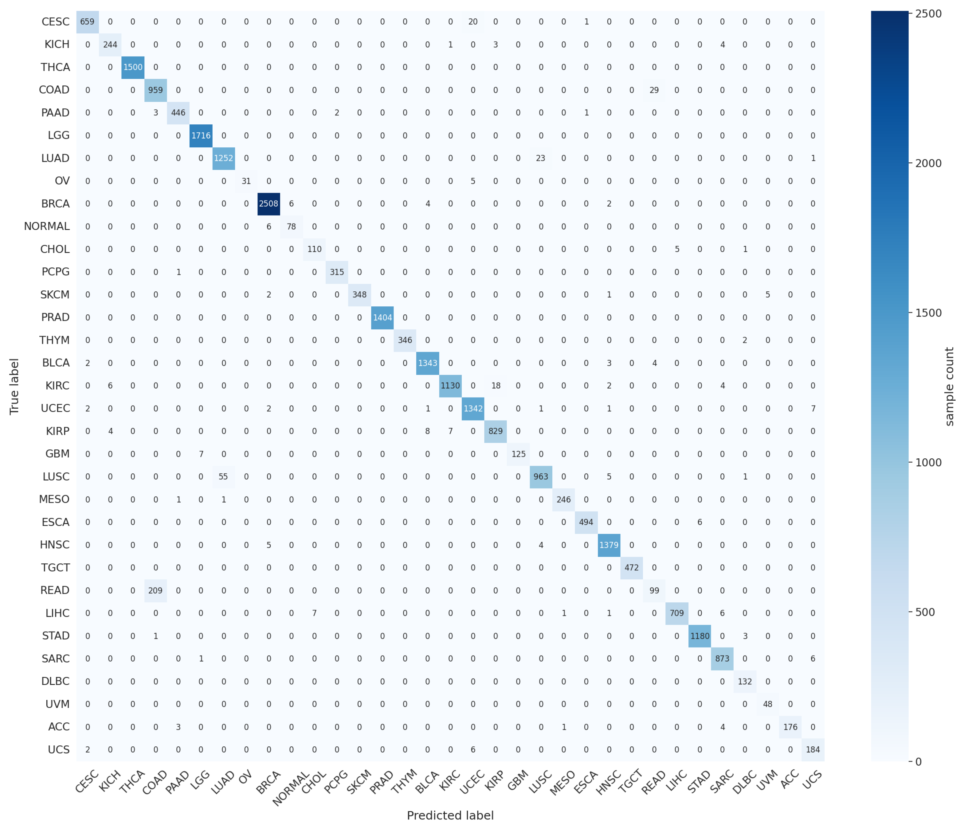
To gain further insights into the model’s classification behaviors, the aggregated confusion matrix from all test set predictions across all 20 runs was plotted (Figure 3).

This matrix revealed that the most frequent misclassifications occurred between cancers that shared the same organ of origin: COAD and READ, LUSC and LUAD, and CESC and UCEC. For gliomas, the model achieved 100% accuracy for LGG and 94.7% for GBM, with all GBM misclassifications assigned to the LGG class, highlighting the model’s ability to consistently identify glioma samples.

4.2. Identification of the Most Important Features

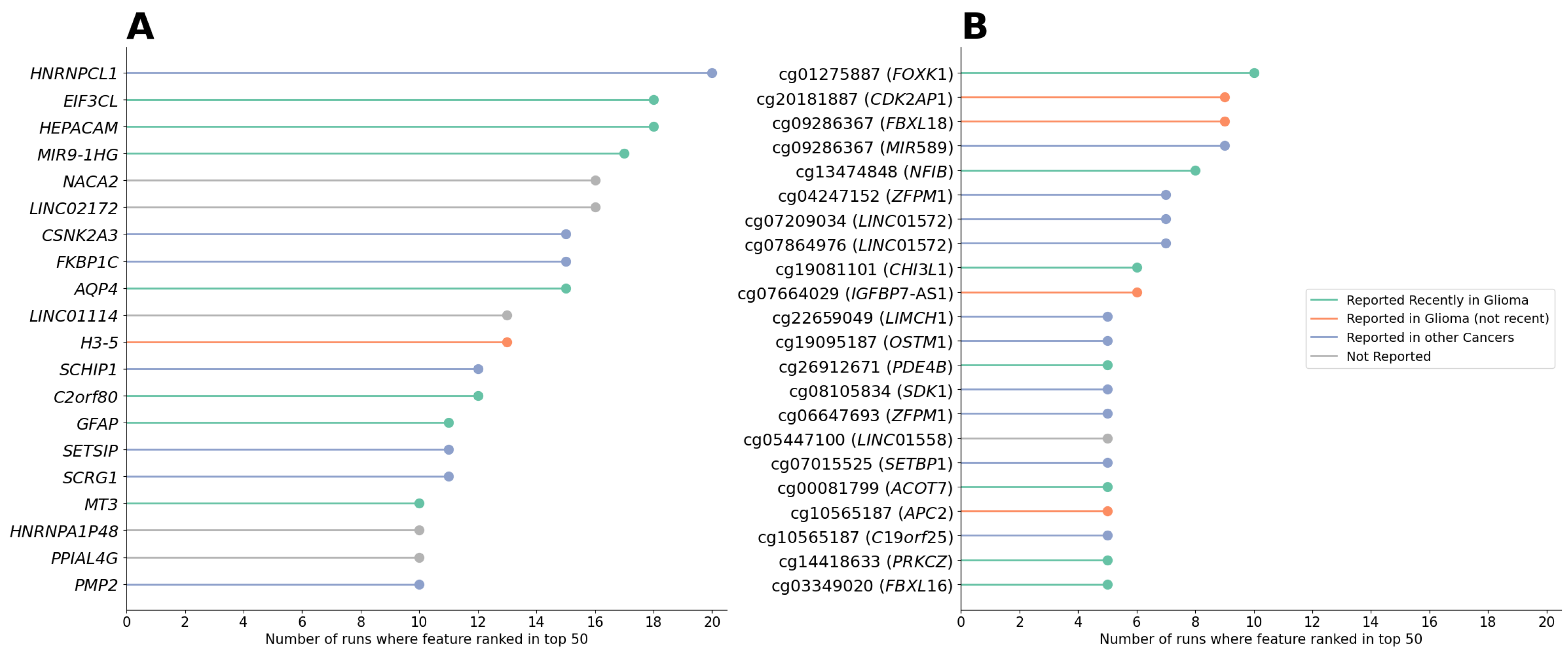
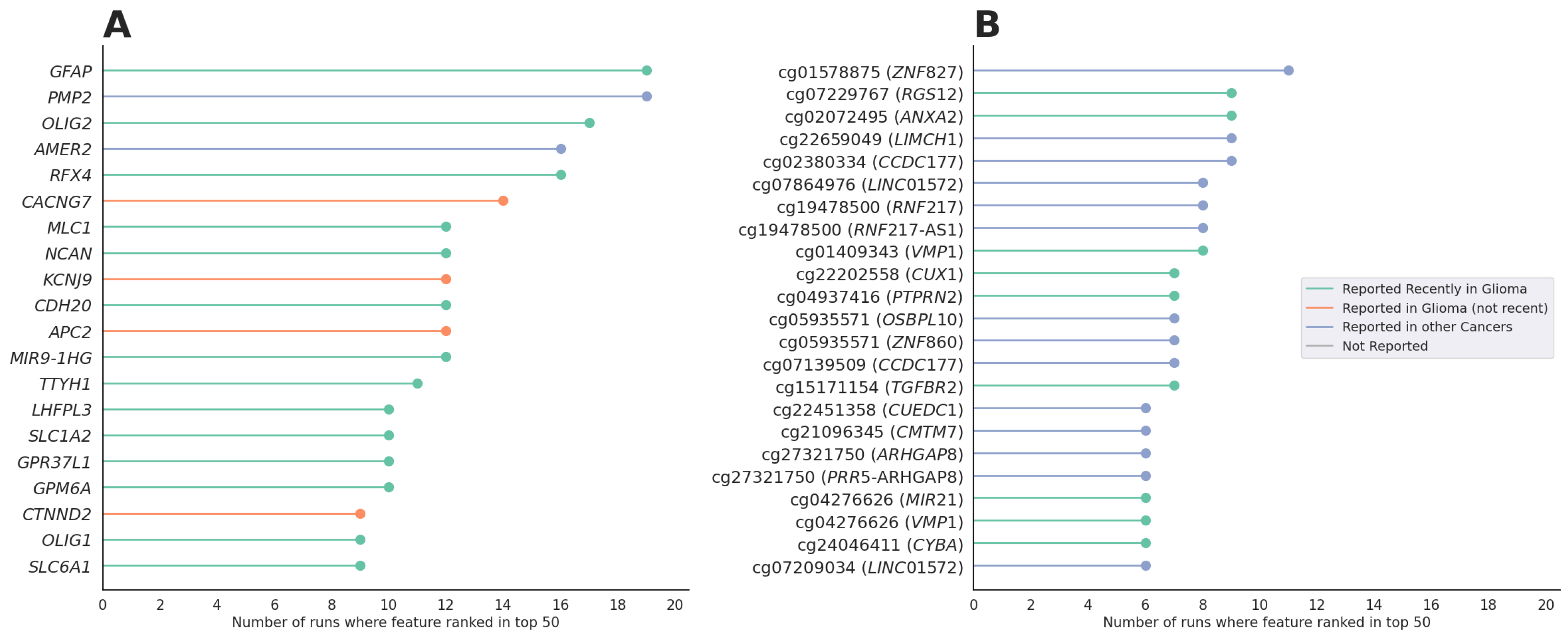
As part of the model evaluation phase for each model run, we identified the most important features associated with each glioma subtype. Figure 4 and Figure 5 show the results for GBM and LGG, respectively. In each figure, panel A corresponds to gene expression features, while panel B corresponds to DNA methylation features. Features were ranked by the number of runs (out of 20) in which they appeared among the top 50 features according to their mean absolute SHAP value. The horizontal bar plots indicate whether the feature has been previously reported in literature according to PubMed: either recently (within the last 5 years), associated with gliomas more generally, associated with other cancer types, or not reported at all.

In GBM, 17 genes were identified as being associated with gliomas, including 5 with recent publications, 19 reported only in other cancer types, and 6 novel candidates that had not been previously described in the literature. For LGG, 27 glioma-related genes were found, 4 of which had recent publications, along with 15 genes linked to other cancers. Gene expression features demonstrated high consistency, with markers such as HNRNPCL1 identified in all 20 runs and GFAP and PMP2 in 19 runs. In contrast, DNA methylation features exhibited greater variability, with the most stable features, cg01578875 (ZNFB27) and cg01275887 (FOXK1), selected in only 11 and 10 out of 20 runs, respectively.

4.3. Differential Expression Analysis Results

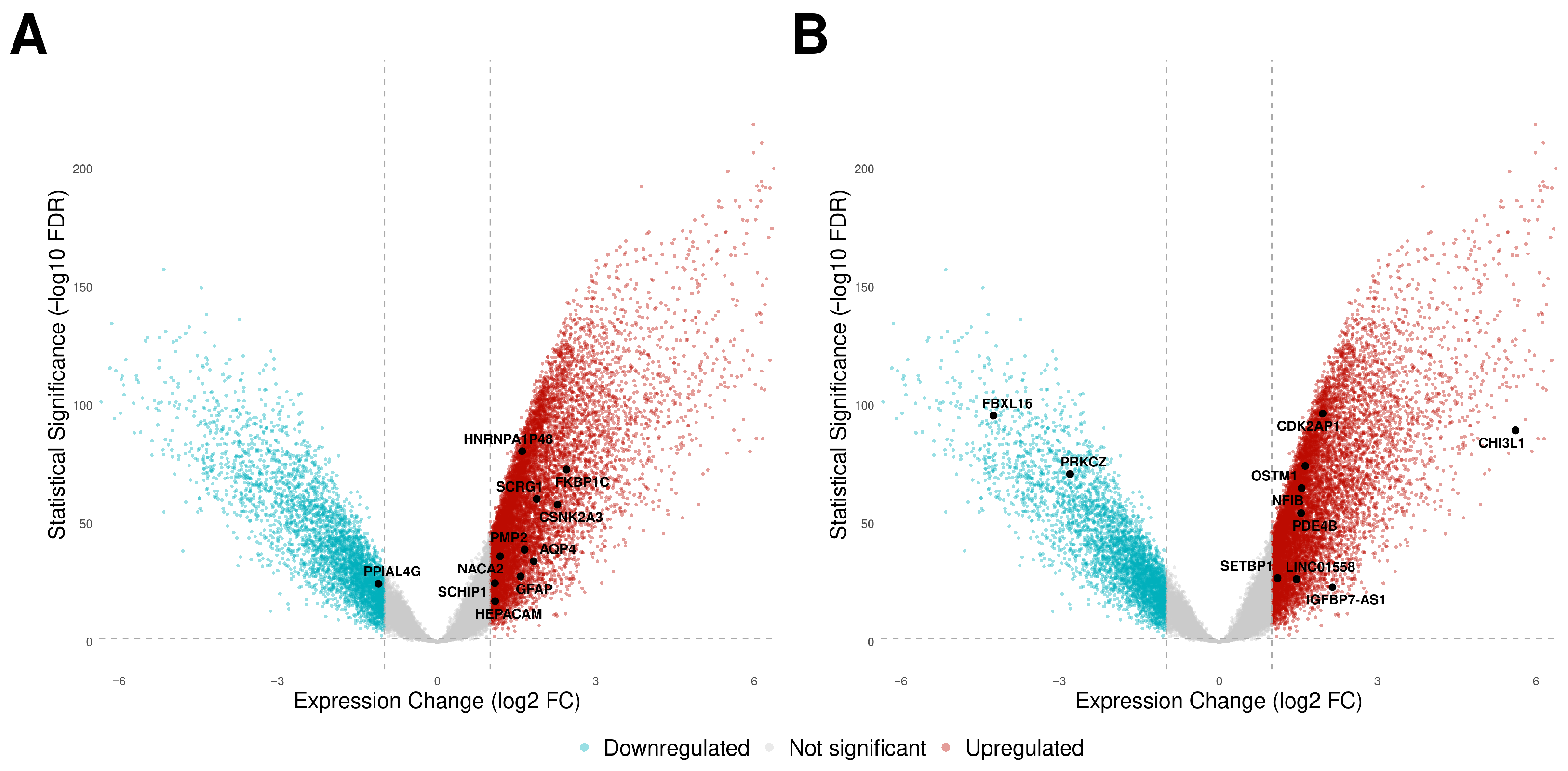
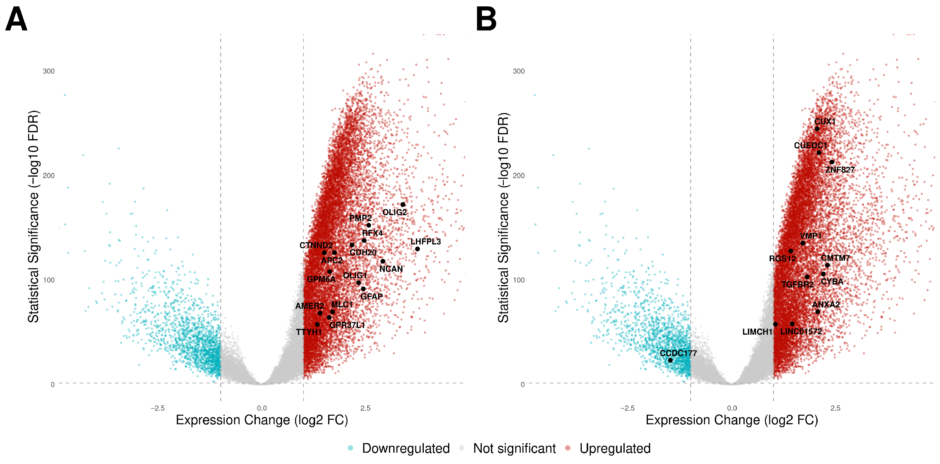
To assess the biological plausibility of the top-ranked features, we performed differential expression analyses comparing tumor versus normal tissue samples for both glioma subtypes. Figure 6 and Figure 7 present the resulting volcano plots for GBM and LGG, respectively.

Figure 4. Top features selected for glioblastoma multiforme. Features ((A) gene expression; (B) DNA methylation) are ranked by their frequency of appearance across the top 50 across 20 model runs. Line colors denote: if the feature has been reported in glioma studies in the last 5 years (green); if it has ever been reported in glioma studies (orange); if it has been reported in studies of other cancer types (blue); and if it has never been reported (grey), based on the PubMed database.

Figure 4. Top features selected for glioblastoma multiforme. Features ((A) gene expression; (B) DNA methylation) are ranked by their frequency of appearance across the top 50 across 20 model runs. Line colors denote: if the feature has been reported in glioma studies in the last 5 years (green); if it has ever been reported in glioma studies (orange); if it has been reported in studies of other cancer types (blue); and if it has never been reported (grey), based on the PubMed database.

Figure 5. Top features selected for low-grade gliomas. Features ((A) gene expression; (B) DNA methylation) are ranked by their frequency of appearance across the top 50 across 20 model runs. Line colors denote: if the feature has been reported in glioma studies in the last 5 years (green); if it has ever been reported in glioma studies (orange); if it has been reported in studies of other cancer types (blue); if it has never been reported (grey), based on the PubMed database.

Figure 5. Top features selected for low-grade gliomas. Features ((A) gene expression; (B) DNA methylation) are ranked by their frequency of appearance across the top 50 across 20 model runs. Line colors denote: if the feature has been reported in glioma studies in the last 5 years (green); if it has ever been reported in glioma studies (orange); if it has been reported in studies of other cancer types (blue); if it has never been reported (grey), based on the PubMed database.

In GBM, 11 of the 20 top gene expression features were found significantly differentially expressed, with 10 upregulated and 1 downregulated in tumor tissue compared to normal samples. Among DNA methylation-associated genes, 10 of 22 were differentially expressed, with 8 upregulated and 2 downregulated. In the LGG cohort, 15 of the 20 top gene expression features were significantly differentially expressed and upregulated in tumor samples. For DNA methylation-linked genes, 12 of 23 showed significant differential expression, with 11 upregulated and 1 downregulated.

Figure 6. Differential expression analysis results for glioblastoma multiforme. (A) Volcano plot for genes corresponding to top gene expression features. (B) Volcano plot for genes linked to top DNA methylation probes. Red dots represent positively expressed genes, blue dots represent negatively expressed genes, and grey dots represent non-significant genes (FDR-adjusted p-value ≥ 0.05 or $|{log}_2\mathrm{FC}|<1$).

Figure 6. Differential expression analysis results for glioblastoma multiforme. (A) Volcano plot for genes corresponding to top gene expression features. (B) Volcano plot for genes linked to top DNA methylation probes. Red dots represent positively expressed genes, blue dots represent negatively expressed genes, and grey dots represent non-significant genes (FDR-adjusted p-value ≥ 0.05 or $|{log}_2\mathrm{FC}|<1$).

Figure 7. Differential expression analysis for low-grade gliomas. (A) Volcano plot for genes corresponding to top gene expression features. (B) Volcano plot for genes linked to top DNA methylation probes. Red dots represent positively expressed genes, blue dots represent negatively expressed genes, and grey dots represent non-significant genes (FDR-adjusted p-value ≥ 0.05 or $|{log}_2\mathrm{FC}|<1$).

Figure 7. Differential expression analysis for low-grade gliomas. (A) Volcano plot for genes corresponding to top gene expression features. (B) Volcano plot for genes linked to top DNA methylation probes. Red dots represent positively expressed genes, blue dots represent negatively expressed genes, and grey dots represent non-significant genes (FDR-adjusted p-value ≥ 0.05 or $|{log}_2\mathrm{FC}|<1$).

4.4. DNA Methylation Analysis Results

Given the complex relationship between CpG probes and their associated genes, we examined, for each glioma subtype, the methylation levels ($\beta$-values) of the top-ranked DNA methylation features in both tumor and normal samples, with the goal of uncovering information that may support our hypothesis-driven interpretations. For each probe, we also annotated its genomic context relative to the TSS and its position relative to CpG islands.

Table 7. Top-ranked differentially methylated features in glioblastoma multiforme. The table displays the selected DNA methylation features alongside their mean $\Delta \beta$-value (difference in mean $\beta$-values between tumor and normal samples). For each probe, its corresponding gene, genomic context(s), and CGI position are identified.

Probe ID	Gene	Genomic Context	CGI Position	$\Delta \mathit{\beta }$-Value
cg19081101	CHI3L1	TSS1500	NA	−0.6281
cg03349020	FBXL16	Gene body	Island	0.3937
cg05447100	LINC01558	Gene body	NA	−0.3027
cg13474848	NFIB	Gene body	S_Shore	−0.2874
cg20181887	CDK2AP1	Gene body; TSS1500	N_Shore	−0.2463
cg14418633	PRKCZ	Gene body; TSS1500	Island	0.1938
cg09286367	FBXL18	Gene body	S_Shore	−0.1743
cg09286367	MIR589	TSS200	S_Shore	−0.1743
cg00081799	ACOT7	Gene body	NA	0.1362
cg22659049	LIMCH1	Gene body	S_Shore	0.1040
cg06647693	ZFPM1	Gene body	Island	−0.1035
cg04247152	ZFPM1	Gene body	Island	−0.0946
cg07015525	SETBP1	Gene body	S_Shore	0.0944
cg08105834	SDK1	Gene body	NA	−0.0601
cg07864976	LINC01572	Gene body	NA	0.0558
cg07209034	LINC01572	Gene body	NA	0.0385
cg19095187	OSTM1	Gene body	S_Shore	0.0279
cg01275887	FOXK1	Gene body	NA	−0.0188
cg07664029	IGFBP7-AS1	Gene body	NA	−0.0070
cg26912671	PDE4B	Gene body	NA	−0.0063
cg10565187	C19orf25	Gene body	Island	−0.0049
cg10565187	APC2	Gene body	Island	−0.0049

and

Table 8. Top-ranked differentially methylated features in low-grade gliomas. The table displays the selected DNA methylation features alongside their mean $\Delta \beta$-value (difference in mean $\beta$-values between tumor and normal samples). For each probe, its corresponding gene, genomic context(s), and CGI position are reported.

Probe ID	Gene	Genomic Context	CGI Position	$\Delta \mathit{\beta }$
cg05935571	OSBPL10	Gene body; TSS1500	Island	0.6960
cg05935571	ZNF860	Gene body; TSS200	Island	0.6960
cg15171154	TGFBR2	Gene body; TSS200	NA	−0.6312
cg22451358	CUEDC1	Gene body	N_Shore	0.6088
cg19478500	RNF217	Gene body	S_Shore	0.5981
cg19478500	RNF217-AS1	TSS1500	S_Shore	0.5981
cg04276626	VMP1	Gene body	NA	0.3385
cg04276626	MIR21	TSS200	NA	0.3385
cg27321750	PRR5-ARHGAP8	Gene body	Island	0.1864
cg27321750	ARHGAP8	TSS1500	Island	0.1864
cg21096345	CMTM7	TSS1500	N_Shore	0.1549
cg04937416	PTPRN2	Gene body	S_Shore	0.1502
cg07139509	CCDC177	Gene body	Island	−0.1401
cg01409343	VMP1	Gene body	NA	0.1052
cg22202558	CUX1	Gene body	NA	0.0590
cg24046411	CYBA	TSS1500; TSS200	S_Shore	0.0473
cg22659049	LIMCH1	Gene body	S_Shore	0.0361
cg02072495	ANXA2	Gene body	N_Shore	−0.0324
cg02380334	CCDC177	Gene body	Island	−0.0204
cg07864976	LINC01572	Gene body	NA	0.0168
cg01578875	ZNF827	Gene body	NA	0.0071
cg07229767	RGS12	Gene body	N_Shelf	−0.0055
cg07209034	LINC01572	Gene body	NA	0.0055

summarize these findings for the GBM and LGG cohorts, respectively.

Applying a threshold of $|\Delta \beta |>0.2$ to the GBM cohort (Table 7), we identified five probes that displayed significant methylation changes: cg19081101 (CHI3L1), cg03349020 (FBXL16), cg05447100 (LINC01558), cg13474848 (NFIB) and cg20181887 (CDK2AP1). Among these, cg19081101 displayed the most pronounced hypomethylation $(\Delta \beta =-0.63)$, while cg03349020 exhibited the most significant hypermethylation $(\Delta \beta =0.39)$. To assess whether these alterations are GBM-specific or shared across glioma grades, we examined the methylation differences of these five probes in LGG samples against the same normal reference. Three probes, cg03349020 (FBXL16), cg13474848 (NFIB), and cg20181887 (CDK2AP1) exhibited comparable $\Delta \beta$ values in both cohorts. In contrast, cg19081101 (CHI3L1) displayed substantially attenuated hypomethylation in LGG ($\Delta \beta =-0.22$) compared to GBM ($\Delta \beta =-0.63$). Similarly, cg05447100 (LINC01558) also displayed less methylation difference in LGG ($\Delta \beta =-0.18$) compared to GBM ($\Delta \beta =-0.30$).

In the LGG cohort (Table 8), five probes also showed significant methylation differences: cg05935571 (OSBPL10 and ZNF860), cg15171154 (TGFBR2), cg22451358 (CUEDC1), cg19478500 (RNF217 and RNF217-AS1) and cg04276626 (VMP1 and MIR21). Among these, cg05935571 showed the most pronounced hypermethylation ($\Delta \beta =0.70$), while cg15171154 displayed the most pronounced hypomethylation ($\Delta \beta =-0.63$). As performed for the GBM cohort, we examined the $\Delta \beta$ values of these probes in GBM samples against the same normal reference. While cg15171154 (TGFBR2) exhibited comparable hypomethylation in both cohorts, the remaining four probes displayed notable differences between cohorts. In particular, cg05935571 (OSBPL10 and ZNF860), cg22451358 (CUEDC1), and cg19478500 (RNF217 and RNF217-AS1) showed reduced hypermethylation in GBM, ($\Delta \beta =0.41$, $\Delta \beta =0.33$, and $\Delta \beta =0.25$, respectively) compared to LGG ($\Delta \beta =0.70$, $\Delta \beta =0.61$, and $\Delta \beta =0.60$). Most notably, cg04276626 (VMP1 and MIR21) that had exhibited pronounced hypermethylation in LGG ($\Delta \beta =0.34$) showed negligible change in GBM ($\Delta \beta =-0.04$), representing an LGG-specific alteration. Conversely, cg02072495 (ANXA2), which showed negligible methylation change in LGG ($\Delta \beta =-0.03$), displayed substantial hypomethylation in GBM ($\Delta \beta =-0.42$), indicating a GBM-specific epigenetic change.

4.5. Comparative Analysis of Bayesian Networks

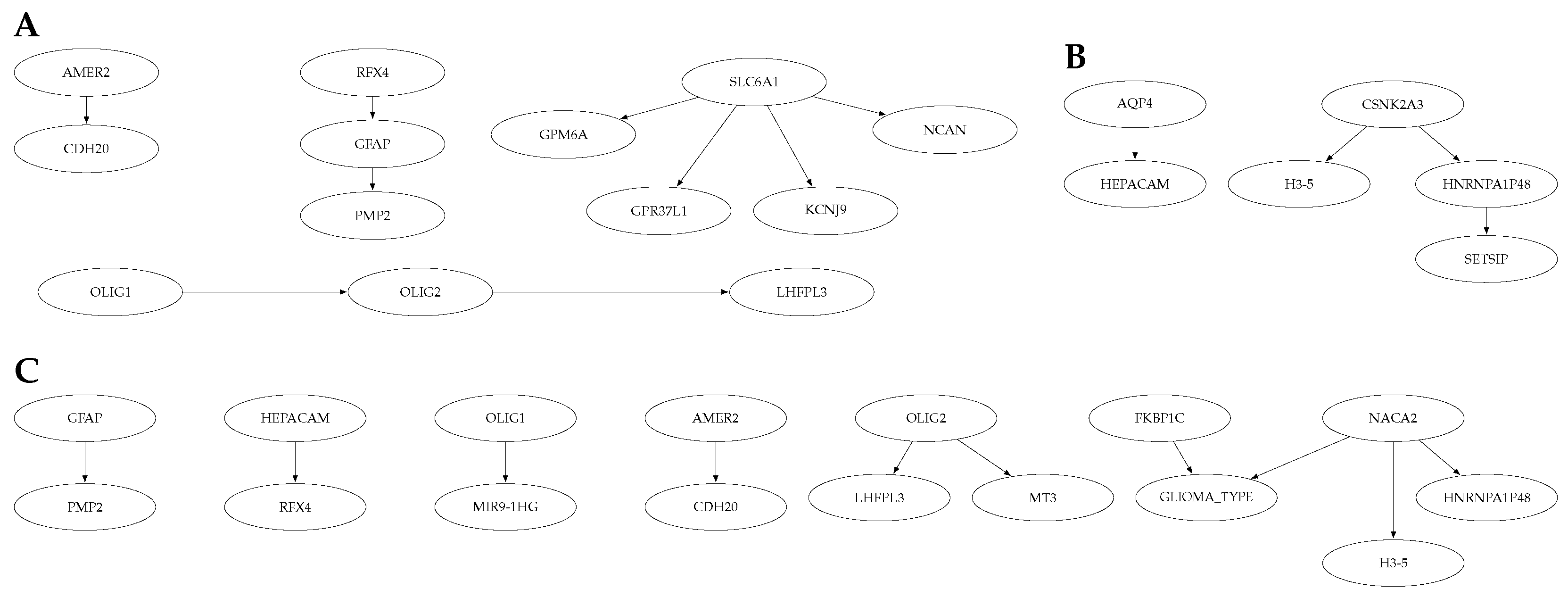
Following the methods described in Section 3.6, three networks were generated for the gene expression data. Figure 8 presents these results.

Analysing the LGG network, depicted in Figure 8A, we can identify several clusters originating from the parent nodes SLC6A1, RFX4, OLIG1, and AMER2. Among these, SLC6A1 is modeled as a regulatory hub, acting as a parent node to four child nodes. Across the network, there is a strong positive correlation between parent and child nodes: when a parent node is set to “high” expression, the child node’s probability of also being “high” increases substantially, and there is also a moderate increase in the “medium” probability. Conversely, “very low” parent node expression leads to a corresponding increase in the child’s “very low” probability. This effect is particularly pronounced along the OLIG1→OLIG2 edge, where “high” expression of OLIG1 corresponds to a 71% probability of “high” and a 25% probability of “medium” expression for OLIG2. For “very low” values of OLIG1, OLIG2 exhibits an 82% probability of “very low” and 17% of “low” expression. A similar pattern with comparable strength is observed along the AMER2→CDH20 and SLC6A1→KCNJ9 edges.

In the GBM-specific network (Figure 8B), this correlation pattern persists. The network is smaller, comprising only two independent clusters. The effect is particularly strong at the CSNK2A3 node, where “high” expression corresponds to approximately 80% probability of “high” and 13% probability of “medium” expression in both of its child nodes, H3-5 and HNRNPA1P48.

In the joint network (Figure 8C), we can also observe the same pattern. Three edges from the LGG network persist in the joint network: AMER2→CDH20, GFAP→PMP2, and OLIG2→LHFPL3, appearing with comparable CPT values. In this network, the node NACA2 presents the strongest correlation with its child nodes, with “high” expression of NACA2 corresponding to a 90.7% and 84.8% probability of “high” expression for H3-5 and HNRNPA1P48, respectively. The “GLIOMA_TYPE” node is directly influenced by two parent genes: NACA2 and FKBP1C. Concurrent “high” expression of both genes yields a 99.2% probability of the sample being classified as GBM. In contrast, when both genes exhibit “very low” expression, the probability of the sample being LGG reaches 99.6%.

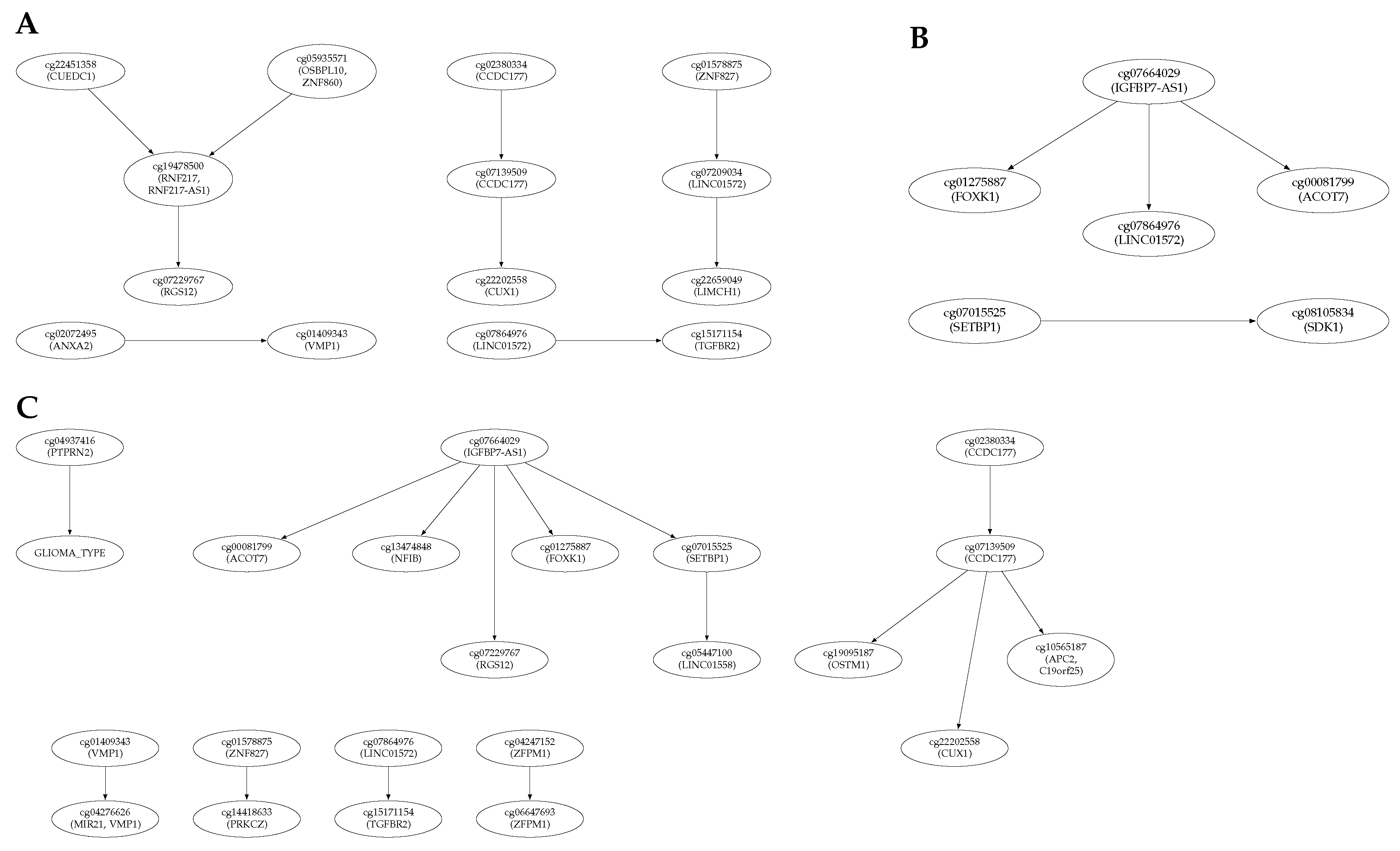
In a similar approach, Figure 9 presents the three BNs generated for the DNA methylation data.

For the DNA methylation data, the LGG network illustrated in Figure 9A presents distinct clusters. Notably, the edge cg02380334→cg07139509 connects two probes mapping to the same gene (CCDC177), indicating that the network successfully captured intra-gene methylation coordination. In a similar fashion to the gene expression networks, there is a strong positive correlation between parent and child nodes: “high” methylation at a parent node causes substantially higher probability of “high” methylation at its child nodes, while “very low” parent values leads to a corresponding increase in the “very low” probability of the child. The GBM-specific network (Figure 9B) is smaller, comprising only two independent clusters. In this netwrok the probe cg07664029 (IGFBP7-AS1) acts as a regulatory hub with three child nodes and the same positive correlation pattern persists across all edges.

In the joint network (Figure 9C), several edges connect probes mapping to the same gene: cg01409343→cg04276626 (VMP1), cg04247152→cg06647693 (ZFPM1), and cg02380334 →cg07139509 (CCDC177). At the same time, edges from both subtype-specific networks persist in this joint network. From the LGG network, the edge chain cg02380334→cg07139509→ cg22202558 and the edge cg07864976→cg15171154 are retained with identical CPT values. From the GBM network, the edges cg07664029→cg00081799 and cg07664029→cg01275887 also persist with identical CPT values. The positive correlation pattern observed across all previous networks is maintained for this network as well. The “GLIOMA_TYPE” node is directly influenced by a single parent probe, cg04937416 (PTPRN2). “High” or “medium” methylation of this probe corresponds to a 97% probability of the sample being classified as LGG.

5. Discussion

In this study, we developed a comprehensive framework for glioma biomarker discovery that integrates a H-VAE with SHAP interpretability to identify molecular features associated with glioma subtypes. The framework’s pipeline is strengthened by a multi-layered validation strategy of the identified biomarkers, including DEA, DNA methylation analysis, and BN modeling to reveal potential relationships among them. The H-VAE demonstrated high performance in the pan-cancer classification task, achieving a near-perfect AUC of $0.9993$, which represents a notable improvement over the original CustOmics model (AUC of $0.9918$). We attribute this improvement to our two-stage hyperparameter optimization strategy (see Section 3.3), where AUC was explicitly defined as the optimization objective. This result serves as strong evidence of the powerful functionalities of the Optuna optimization framework. However, this near-perfect performance must be contextualized within the inherent dataset structure and high class separability of pan-cancer studies. Because samples originating from disparate organ systems possess distinct multi-omics profiles, most cancer classes are biologically well-separated within the feature space, which intrinsically facilitates high classification accuracy.

Figure 9. Consensus Bayesian networks for DNA methylaion data. Figures (A–C) illustrate the BN derived from (A) LGG samples, (B) GBM samples, and (C) GBM and LGG samples. Each node corresponds to a feature selected by the H-VAE model. Direct edges denote the conditional dependencies learned by the BN.

Figure 9. Consensus Bayesian networks for DNA methylaion data. Figures (A–C) illustrate the BN derived from (A) LGG samples, (B) GBM samples, and (C) GBM and LGG samples. Each node corresponds to a feature selected by the H-VAE model. Direct edges denote the conditional dependencies learned by the BN.

Beyond its high performance, the model’s behavior revealed a strong alignment with established biological knowledge. Analysis of the aggregated confusion matrix revealed that the most frequent misclassifications occurred between cancer types sharing a common origin organ system, specifically, between COAD and READ, and between LUAD and LUSC. The difficulty in distinguishing COAD from READ is a well-recognized challenge. Due to their shared origin in the large intestine and highly similar molecular profiles, these cancers are often grouped under the collective term CRC [29]. Similarly, although LUAD and LUSC exhibit distinct histological and molecular characteristics [30], they are also known to share common mutations, such as a mutation in the tumor suppressor gene TP53 [31,32], which, coupled with their shared tissue of origin, likely contributed to the observed model misclassifications. A similar pattern is observed in gynecologic cancers, where the model misclassified CESC samples for UCEC samples. Crucially, while the model achieves high accuracy across most cancer types, its reduced performance when subtyping cancers between the same organs of origin, reflects the intrinsic biological ambiguity within these groups.

Investigation into the biological context of the selected features by the H-VAE model, provided intriguing insights. Specifically for the GBM cohort, our framework identified a set of both well-established and novel biomarkers. Among the established markers are GFAP, AQP4, HEPACAM, and CHI3L1, genes with extensive literature supporting their association with glioma biology. Additionally, our model consistently identified the HNRNPCL1 gene as related to GBM. Although HNRNPCL1 has only been identified as a potential biomarker for endometrial cancer [33], our findings suggest its potential involvement in glioma. Among the top-ranked were also EIF3CL and MIR9-1HG. Despite having been reported only once in the context of gliomas [34,35], our results reinforce their potential association with gliomas. Furthermore, the model uncovered six novel candidate biomarkers for GBM: LINC02172, NACA2, LINC01114, HNRNPA1P48, PPIAL4G, and LINC01558. Among these, differential expression analysis showed that NACA2, HNRNPA1P48, and LINC01558 were overexpressed in GBM samples. While there are currently no literature reports connecting these specific biomarkers to gliomas, database annotations reveal interesting insights [36]. Notably, the long non-coding RNA LINC01114 is associated with childhood ependymoma, a primary glial tumor of the central nervous system. Additionally, HNRNPA1P48 is associated with frontotemporal dementia, and PPIAL4G with epileptic encephalopathies, both of which are neurological disorders. Furthermore, HNRNPA1P48 is predicted to regulate mRNA splicing via the spliceosome, a critical mechanism in the development of the brain, while both PPIAL4G and NACA2 are involved in cellular protein folding.

Analysis of the DNA methylation profiles of the selected probes for GBM revealed several noteworthy patterns. The probe cg19081101, mapping to the promoter region (TSS1500) of CHI3L1, exhibited the strongest hypomethylation in GBM ($\Delta \beta =-0.628$) which coincided with a marked upregulation of the gene in GBM samples, in our DEA. This aligns with studies reporting that CHI3L1 influences several mechanisms crucial to GBM progression, potentially being a therapeutic target [37]. More notably, in LGG, the hypomethylation of this probe was considerably attenuated ($\Delta \beta =-0.223$), and in our DEA, CHI3L1 showed no significant expression change, suggesting that the degree of methylation of this probe may contribute to the transcriptional activation of CHI3L1. The probe cg03349020, located within a CpG island in the gene body of FBXL16, was found to be similarly hypermethylated in both GBM and LGG. Concurrently, our DEA showed that this gene is downregulated in both cohorts, with the effect being substantially more pronounced in GBM. FBXL16 is known to function as a component of E3 ubiquitin ligase complexes, which are known to drive pro-survival signaling and therapy resistance in glioblastoma [38]. These findings point to a possible relationship between the hypermethylation of cg03349020 and the silencing of this gene. Finally, the probe cg05447100, mapping to the gene body of LINC01558, displayed significant hypomethylated only in GBM, which was accompanied by an upregulation of this gene in the same cohort. In LGG however, the probe showed no significant hypomehtylation nor differential expression, raising the possibility that the methylation state of this probe may influence LINC01558.

Shifting to the LGG cohort, our model found a larger set of glioma-associated genes, though no novel biomarkers were identified. We believe this difference is mainly attributed to the difference in the number of samples between the two datasets, where we used 200 samples for the LGG SHAP values calculation and only 33 for the GBM cohort. This larger sample size potentially allowed the model to better estimate the SHAP values for the LGG cohort, which is reflected in the increased number of glioma-associated genes identified. These include GFAP, OLIG1, OLIG2, SLC1A2, MIR21, ANXA2, and TGFBR2. Notably, the model highlighted PMP2 in both GBM and LGG. Since PMP2 encodes a myelin-associated protein [36], its consistent identification across both glial-derived tumors is intriguing. Among the top LGG ranked features was AMER2, which is a known negative regulator of the Wnt/$\beta$-catenin signaling pathway, whose dysregulation is an established driver of glioma pathogenesis, strongly suggesting AMER2’s specific involvement in glioma biology.

The DNA methylation analysis for LGG revealed two probes of interest. The probe cg05935571, mapping to the promoter regions of both OSBPL10 (TSS1500) and ZNF860 (TSS200) within a CpG island, exhibited the strongest hypermethylation ($\Delta \beta =0.696)$ despite neither gene showing significant differential expression in this cohort. In GBM, the hypermethylation at this probe was less pronounced ($\Delta \beta =0.414$). However, our DEA revealed that OSBPL10 was significantly upregulated in GBM samples, suggesting a possible relation between the strengh of methylation of this probe and suppression of transcription at this site. In an opposite way, the probe cg15171154, mapping to the promoter region (TSS200) of TGFBR2, was strongly hypomethylated in both LGG and GBM, and our DEA identified the gene as upregulated in both cohorts. This is consistent with previous reports that identified TGFBR2 as upregulated in both glioma grades [39], and suggests a possible relation between the probe cg15171154 and the expression of TGFBR2 in gliomas.

The constructed BNs provided a complementary perspective to our previous findings. In the joint gene expression network, the node defining the glioma subtype was directly influenced by the genes NACA2 and FKBP1C. Strikingly, high expression of both genes corresponded to a $99.2\%$ probability of the sample being classified as GBM, while very low expression of both resulted in a $99.6\%$ probability of LGG. This direct conditional relation further supports the potential relevance of NACA2 as a candidate biomarker in gliomas. At the same time, while no literature currently reports a connection between FKBP1C and gliomas, our findings suggest a possible involvement. In the LGG gene expression network, the model captured a strong correlation between OLIG1 and OLIG2, where high expression of OLIG1 corresponded to high expression of OLIG2. This further demonstrates the capability of BNs to recover established biological relationships, as OLIG1 and OLIG2 as OLIG1 and OLIG2 are closely related genes from the same chromosome and OLIG2 is known to be highly expressed in all diffuse gliomas [40]. Moreover, the network modeled relations supported by existing literature. Specifically, the model identified the co-regulation of SLC6A1 and GPM6A, both of which are known to participate in the Synaptic Neuron and Astrocyte Programme [41]. Additionally, it linked SLC6A1, which encodes the GAT-1 protein expressed in astrocytes [42], to GPR37L1, which has been implicated in astrocyte maturation [43]. With respect to the DNA methylation networks, the model successfully captured intra-gene methylation coordination for CCDC177, VMP1, and ZFPM1 in the joint network, where probes mapping to the same gene were connected by direct edges. Furthermore, in this joint methylation network, the probe cg04937416 (PTPRN2) was modelled as directly influencing the glioma subtype, with high or medium methylation values corresponding to a $97\%$ probability of LGG classification. In this context, recent work has identified PTPRN2 as potentially involved in GBM cell migration [44].

To assess the potential clinical relevance of the identified biomarkers, Kaplan–Meier survival analyses were performed on the combined TCGA-GBM and TCGA-LGG cohort, stratified by median expression. For gene expression data, high expression of CHI3L1, FKBP1C, LINC01114, HNRNPCL1, NACA2, PPIAL4G, HNRNPA1P48, EIF3CL, LINC02172, TGFBR2, and LINC01558 was significantly associated with worse overall survival (log-rank p < 0.0001), whereas low expression of AMER2 and MIR9-1HG was associated with reduced survival. For DNA methylation data, low methylation $\beta$-values at the probes cg19081101 (CHI3L1), cg05935571 (OSBPL10 and ZNF860), cg04937416 (PTPRN2), and cg04276626 (VMP1 and MIR21) were associated with significantly worse survival, while high $\beta$-values at cg15171154 (TGFBR2) were associated with reduced survival time. To evaluate the reproducibility of these findings in an external dataset, we queried the CGGA survival analysis tool [45] for the gene expression biomarkers found significant in our analysis. Of the seven biomarkers available on the CGGA platform, CHI3L1, FKBP1C, HNRNPCL1, NACA2, HNRNPA1P48, EIF3CL, TGFBR2, and AMER2, five were confirmed as significant: CHI3L1 (p < 0.0001), TGFBR2 (p < 0.0001), AMER2 (p < 0.0001), FKBP1C (p = 0.00028), and HNRNPCL1 (p = 0.0011), all exhibiting the same directional relationship between expression and survival as observed in our survival analysis. Crucially, the fact that AMER2, FKBP1C, and HNRNPCL1, which had only been previously associated with other cancer types, were found to be prognostically significant in both TCGA and CGGA glioma cohorts further reinforces their potential involvement in glioma biology.

Although promising, MOHVAE-B has its limitations. Firstly, despite employing the TOIL recompute dataset and ensuring platform consistency to mitigate technical variations, residual cross-cohort confounding may persist. Because tumor and normal samples originate from distinct databases (TCGA vs. GTEx and GEO), perfect confounding between biological condition and data source cannot be completely eliminated. This residual batch effect must be taken into account when interpreting the biological validation of our results. Secondly, patient-level splitting was not strictly enforced during cross-validation, which could potentially lead to optimistic performance estimates through data leakage across folds. However, the practical impact of this issue is expected to be minimal, as only 20 patients out of the 6003 in the final cohort contribute more than a single sample to the dataset. Thirdly, the use of bulk TCGA data may overlook intra-tumoral heterogeneity. Fourthly, the small sample size of the GBM cohort available for the H-VAE training step and SHAP interpretation ($n=33$) remains a significant limitation, as it affects the stability of SHAP value estimation. Consequently, the biomarker candidates derived for this cohort must be interpreted with caution. In addition, the strict methylation feature filtering might have excluded relevant CpG sites. Finally, because our framework relies on features derived solely from mathematical and computational models, it can only serve as a hypothesis-generating framework. While tools like SHAP and BNs can rank features and highlight probabilistic dependencies, respectively, they cannot establish biological causality. Therefore, additional experimental validation is required to distinguish candidate biomarkers from truly causal biomarkers and represents a crucial next step toward confirming the biological and clinical relevance of our findings, particularly with regard to the six completely novel GBM biomarker candidates identified in this study.

6. Conclusions

In this study, we introduced MOHVAE-B, a framework that integrates an interpretable H-VAE with BNs to identify and interpret biomarkers in multi-omics data. Applied to gliomas, MOHVAE-B achieved high predictive performance while revealing both established and novel biomarkers. In particular, the H-VAE uncovered six new GBM biomarker candidates (LINC02172, NACA2, LINC01114, HNRNPA1P48, PPIAL4G, and LINC01558) and highlighted HNRNPCL1 and AMER2 as promising markers for GBM and LGG, respectively. LINC01572 and PMP2 were identified in both glioma subtypes, becoming particularly strong candidates for a potential role in glioma pathogenesis. Through our integrated methylation and differential expression analyses, we identified epigenetic patterns that may underlie the transcriptional activation of genes. Specifically, the probes cg19081101 (CHI3L1), cg03349020 (FBXL16), and cg05935571 (OSBPL10 and ZNF860) warrant further investigation into their regulatory roles.

Furthermore, the constructed BNs provided additional valuable insights complementing the biomarkers identified by the H-VAE. In the joint gene expression network, NACA2 and FKBP1C were modeled as direct parents of the glioma subtype node, where concurrent “high” expression of both genes corresponded to a $99.2\%$ probability of GBM classification, while very low expression of both resulted in a $99.6\%$ probability of LGG. This further reinforces NACA2 as a novel candidate of interest in gliomas, while FKBP1C, whose prognostic role was confirmed in both TCGA and CGGA, emerges as a potential glioma-related biomarker. In the joint methylation network, the probe cg04937416 (PTPRN2) was identified as directly influencing the glioma subtype, with “high” or “medium” methylation corresponding to a $97\%$ probability of LGG classification, suggesting it as a candidate of interest for further study.

Overall, MOHVAE-B provides an interpretable and extensible framework for biomarker discovery. While external validation in this study was limited to survival analysis using the CGGA cohort, comprehensive model-level validation on independent datasets remains an important direction for future work. Additionally, we suggest applying MOHVAE-B to other TCGA cancer cohorts or experimenting with single-cell datasets. The full codebase and results from this study are publicly available at https://github.com/sysbiomed/MOHVAE-B (accessed on 4 March 2026).

References

1. Goodenberger, M.L.; Jenkins, R.B. Genetics of adult glioma. Cancer Genet. 2012, 205, 613–621. [Google Scholar] [CrossRef]
2. Ostrom, Q.T.; Cioffi, G.; Waite, K.; Kruchko, C.; Barnholtz-Sloan, J.S. CBTRUS Statistical Report: Primary Brain and Other Central Nervous System Tumors Diagnosed in the United States in 2014–2018. Neuro-Oncology 2021, 23, iii1–iii105. [Google Scholar] [CrossRef]
3. Louis, D.N.; Perry, A.; Wesseling, P.; Brat, D.J.; Cree, I.A.; Figarella-Branger, D.; Hawkins, C.; Ng, H.K.; Pfister, S.M.; Reifenberger, G.; et al. The 2021 WHO Classification of Tumors of the Central Nervous System: A summary. Neuro-Oncology 2021, 23, 1231–1251. [Google Scholar] [CrossRef]
4. TCGA Research Network. The Cancer Genome Atlas Pan-Cancer Analysis Project. Nat. Genet. 2013, 45, 1113–1120. [Google Scholar] [CrossRef] [PubMed]
5. Kingma, D.P.; Welling, M. Auto-Encoding Variational Bayes. arXiv 2013, arXiv:1312.6114. [Google Scholar] [CrossRef]
6. Hira, M.T.; Razzaque, M.A.; Angione, C.; Scrivens, J.; Sawan, S.; Sarker, M. Integrated multi-omics analysis of ovarian cancer using variational autoencoders. Sci. Rep. 2021, 11, 6265. [Google Scholar] [CrossRef] [PubMed]
7. Carvalho, A.M.; Roos, T.; Oliveira, A.L.; Myllymäki, P. Discriminative Learning of Bayesian Networks via Factorized Conditional Log-Likelihood. J. Mach. Learn. Res. 2011, 7, 2181–2210. [Google Scholar]
8. Ivanisevic, T.; Sewduth, R.N. Multi-Omics Integration for the Design of Novel Therapies and the Identification of Novel Biomarkers. Proteomes 2023, 11, 34. [Google Scholar] [CrossRef]
9. Vahabi, N.; Michailidis, G. Unsupervised Multi-Omics Data Integration Methods: A Comprehensive Review. Front. Genet. 2022, 13, 854752. [Google Scholar] [CrossRef]
10. Zhang, X.; Zhang, J.; Sun, K.; Yang, X.; Dai, C.; Guo, Y. Integrated multi-omics analysis using Variational Autoencoders: Application to pan-cancer classification. In Proceedings of the 2019 IEEE International Conference on Bioinformatics and Biomedicine (BIBM), San Diego, CA, USA, 18–21 November 2019; pp. 765–769. [Google Scholar] [CrossRef]
11. Withnell, E.; Zhang, X.; Sun, K.; Guo, Y. XOmiVAE: An interpretable deep learning model for cancer classification using high-dimensional omics data. Brief. Bioinform. 2021, 22, bbab315. [Google Scholar] [CrossRef]
12. Lundberg, S.; Lee, S.-I. A Unified Approach to Interpreting Model Predictions. arXiv 2017, arXiv:1705.07874. [Google Scholar] [CrossRef]
13. Franco, E.F.; Rana, P.; Cruz, A.; Calderon, V.V.; Azevedo, V.; Ramos, R.T.; Ghosh, P. Performance Comparison of Deep Learning Autoencoders for Cancer Subtype Detection Using Multi-Omics Data. Cancers 2021, 13, 2013. [Google Scholar] [CrossRef]
14. Simidjievski, N.; Bodnar, C.; Tariq, I.; Scherer, P.; Andres Terre, H.; Shams, Z.; Jamnik, M.; Liò, P. Variational Autoencoders for Cancer Data Integration: Design Principles and Computational Practice. Front. Genet. 2019, 10, 1205. [Google Scholar] [CrossRef]
15. Kuipers, J.; Thurnherr, T.; Moffa, G.; Suter, P.; Behr, J.; Goosen, R.; Christofori, G.; Beerenwinkel, N. Mutational interactions define novel cancer subgroups. Nat. Commun. 2018, 9, 4353. [Google Scholar] [CrossRef]
16. Bu, W.; Mu, H.; Gao, M.; Su, W.; Shi, F.; Wang, Q.; Wang, S.; Kong, Y. Data-driven Bayesian network learning analysis on the regulatory mechanism between carcinogenic genes and immune cells. Clin. Transl. Discov. 2023, 3, e257. [Google Scholar] [CrossRef]
17. Zhang, Q.; Burdette, J.E.; Wang, J.-P. Integrative network analysis of TCGA data for ovarian cancer. BMC Syst. Biol. 2014, 8, 1338. [Google Scholar] [CrossRef] [PubMed]
18. Goldman, M.J.; Craft, B.; Hastie, M.; Repečka, K.; McDade, F.; Kamath, A.; Banerjee, A.; Luo, Y.; Rogers, D.; Brooks, A.N.; et al. Visualizing and interpreting cancer genomics data via the Xena platform. Nat. Biotechnol. 2020, 38, 675–678. [Google Scholar] [CrossRef] [PubMed]
19. Benkirane, H.; Pradat, Y.; Michiels, S.; Cournède, P.H. CustOmics: A versatile deep-learning based strategy for multi-omics integration. PLoS Comput. Biol. 2023, 19, e1010921. [Google Scholar] [CrossRef]
20. Ioffe, S.; Szegedy, C. Batch normalization: Accelerating deep network training by reducing internal covariate shift. PMLR 2015, 37, 448–456. [Google Scholar]
21. He, K.; Zhang, X.; Ren, S.; Sun, J. Delving deep into rectifiers: Surpassing human-level performance on ImageNet classification. arXiv 2015, arXiv:1502.01852. [Google Scholar]
22. Akiba, T.; Sano, S.; Yanase, T.; Ohta, T.; Koyama, M. Optuna: A next-generation hyperparameter optimization framework. In Proceedings of the 25th ACM SIGKDD International Conference on Knowledge Discovery & Data Mining, Anchorage, AK, USA, 4–8 August 2019; pp. 2623–2631. [Google Scholar]
23. The GTEx Consortium. The Genotype-Tissue Expression (GTEx) project. Nat. Genet. 2013, 45, 580–585. [Google Scholar] [CrossRef]
24. Vivian, J.; Rao, A.A.; Nothaft, F.A.; Ketchum, C.; Armstrong, J.; Novak, A.; Pfeil, J.; Narkizian, J.; Deran, A.D.; Musselman-Brown, A.; et al. Toil enables reproducible, open source, big biomedical data analyses. Nat. Biotechnol. 2017, 35, 314–316. [Google Scholar] [CrossRef]
25. Gasparoni, G.; Bultmann, S.; Lutsik, P.; Kraus, T.F.J.; Sordon, S.; Vlcek, J.; Dietinger, V.; Steinmaurer, M.; Haider, M.; Mulholland, C.B.; et al. DNA methylation analysis on purified neurons and glia dissects age and Alzheimer’s disease-specific changes in the human cortex. Epigenetics Chromatin 2018, 11, 41. [Google Scholar] [CrossRef] [PubMed]
26. Divate, M.; Tyagi, A.; Richard, D.J.; Prasad, P.A.; Gowda, H.; Nagaraj, S.H. Deep learning-based pan-cancer classification model reveals tissue-of-origin specific gene expression signatures. Cancers 2022, 14, 1185. [Google Scholar] [CrossRef]
27. Wang, J.; Dai, X.; Luo, H.; Yan, C.; Zhang, G.; Luo, J. MI_DenseNetCAM: A novel pan-cancer classification and prediction method based on mutual information and deep learning model. Front. Genet. 2021, 12, 670232. [Google Scholar] [CrossRef]
28. Hossain, S.M.M.; Khatun, L.; Ray, S.; Mukhopadhyay, A. Pan-cancer classification by regularized multi-task learning. Sci. Rep. 2021, 11, 24252. [Google Scholar] [CrossRef] [PubMed]
29. Lv, J.L.; Tan, Y.J.; Ren, Y.S.; Ma, R.; Wang, X.; Wang, S.Y.; Liu, W.Q.; Zheng, Q.S.; Yao, J.C.; Tian, J.; et al. Procyanidin C1 inhibits tumor growth and metastasis in colon cancer via modulating miR-501-3p/HIGD1A axis. J. Adv. Res. 2024, 60, 215–231. [Google Scholar] [CrossRef] [PubMed]
30. Chen, J.W.; Dhahbi, J. Lung adenocarcinoma and lung squamous cell carcinoma classification, biomarker identification, and gene expression analysis using overlapping feature selection methods. Sci. Rep. 2021, 11, 13323. [Google Scholar] [CrossRef]
31. Li, H.; Yang, L.; Wang, Y.; Wang, L.; Chen, G.; Zhang, L.; Wang, D. Integrative analysis of TP53 mutations in lung adenocarcinoma for immunotherapies and prognosis. BMC Bioinform. 2023, 24, 155. [Google Scholar] [CrossRef]
32. Nu er lan, S.T.E.; Yu, B.; Yang, Y.; Shen, Y.; Xu, B.; Zhan, Y.; Liu, C. Discover mutational differences between lung adenocarcinoma and lung squamous cell carcinoma and search for more effective biomarkers for immunotherapy. Cancer Manag. Res. 2024, 16, 1759–1773. [Google Scholar] [CrossRef]
33. Gao, Y.; Zhang, X.; Wang, T.; Zhang, Y.; Wang, Q.; Hu, Y. HNRNPCL1, PRAMEF1, CFAP74, and DFFB: Common potential biomarkers for sporadic and suspected Lynch syndrome endometrial cancer. Cancer Manag. Res. 2020, 12, 11231–11241. [Google Scholar] [CrossRef]
34. Chen, J.; Lin, Z.; Barrett, L.; Dai, L.; Qin, Z. Identification of new therapeutic targets and natural compounds against diffuse intrinsic pontine glioma. Bioorg. Chem. 2020, 99, 103847. [Google Scholar] [CrossRef]
35. Steponaitis, G.; Dragunaite, R.; Stakaitis, R.; Sharma, A.; Tamasauskas, A.; Skiriute, D. m6A-lncRNA landscape highlights reduced levels of m6A modification in glioblastoma as compared to low-grade glioma. Mol. Med. 2025, 31, 195. [Google Scholar] [CrossRef]
36. Stelzer, G.; Rosen, N.; Plaschkes, I.; Zimmerman, S.; Twik, M.; Fishilevich, S.; Stein, T.I.; Nudel, R.; Lieder, I.; Mazor, Y.; et al. The GeneCards suite: From gene data mining to disease genome sequence analyses. Curr. Protoc. Bioinform. 2016, 54, 1–30. [Google Scholar] [CrossRef]
37. Cyranowski, S.; Zawadzka, M.; Ghosh, M.; Wojtas, B.; Malik, A.R.; Poleszak, K.; Waśniewski, K.; Baluszek, S.; Swatler, J.; Wojnicki, K. Chitinase-3-like protein 1 depletion in glioma cells alters tumor microenvironment and normalizes neovasculature in human glioma xenografts. Cell Commun. Signal. 2026, 24, 103. [Google Scholar] [CrossRef] [PubMed]
38. Humphreys, L.M.; Smith, P.; Chen, Z.; Fouad, S.; D’Angiolella, V. The role of E3 ubiquitin ligases in the development and progression of glioblastoma. Cell Death Differ. 2021, 28, 522–537. [Google Scholar] [CrossRef] [PubMed]
39. Zhou, X.; Li, X.; Wang, R.; Hua, D.; Sun, C.; Yu, L.; Shi, C.; Luo, W.; Jiang, Z.; An, W.; et al. Recruitment of LEF1 by Pontin chromatin modifier amplifies TGFBR2 transcription and activates TGFβ/SMAD signalling during gliomagenesis. Cell Death Dis. 2022, 13, 818. [Google Scholar] [CrossRef]
40. Ligon, K.L.; Alberta, J.A.; Kho, A.T.; Weiss, J.; Kwaan, M.R.; Nutt, C.L.; Louis, D.N.; Stiles, C.D.; Rowitch, D.H. The oligodendroglial lineage marker OLIG2 is universally expressed in diffuse gliomas. J. Neuropathol. Exp. Neurol. 2004, 63, 499–509. [Google Scholar] [CrossRef] [PubMed]
41. Ling, E.; Nemesh, J.; Goldman, M.; Kamitaki, N.; Reed, N.; Handsaker, R.E.; Genovese, G.; Vogelgsang, J.S.; Gerges, S.; Kashin, S. Concerted neuron-astrocyte gene expression declines in aging and schizophrenia. Nature 2024, 627, 604–611. [Google Scholar] [CrossRef]
42. Mermer, F.; Poliquin, S.; Rigsby, K.; Rastogi, A.; Shen, W.; Romero-Morales, A.; Nwosu, G.; McGrath, P.; Demerast, S.; Aoto, J.; et al. Common molecular mechanisms of SLC6A1 variant-mediated neurodevelopmental disorders in astrocytes and neurons. Brain 2021, 144, 2499–2512. [Google Scholar] [CrossRef]
43. Nguyen, T.T.; Camp, C.R.; Doan, J.K.; Traynelis, S.F.; Sloan, S.A.; Hall, R.A. GPR37L1 controls maturation and organization of cortical astrocytes during development. Glia 2023, 71, 1921–1946. [Google Scholar] [CrossRef] [PubMed]
44. Bharadwaj, A.; Sanazzaro, T.; Seidlits, S.K. Investigating the expression of PTPRN2 and MT1X genes in glioblastoma cell migration using hydrogel-based models. Cancer Res. 2025, 85, 1454. [Google Scholar] [CrossRef]
45. Zhao, Z.; Zhang, K.N.; Wang, Q.; Li, G.; Zeng, F.; Zhang, Y.; Wu, F.; Chai, R.; Wang, Z.; Zhang, C.; et al. Chinese Glioma Genome Atlas (CGGA): A comprehensive resource with functional genomic data from Chinese glioma patients. Genom. Proteom. Bioinform. 2021, 19, 1–12. [Google Scholar] [CrossRef]
Figure 1. Phase 1 of the H-VAE training. Representation of the first training phase, showing independent autoencoders per omics modality. Each latent representation space is linked to a classifier network for sample type prediction.
Biomedinformatics 06 00031 g001
Figure 2. Phase 2 of the H-VAE training. In contradiction to phase 1, the modality-specific latent representations are concatenated and passed into a central Variational Autoencoder to learn a shared latent space. The mean vector ( μ ) from the central encoder is connected to a common classifier network for sample type prediction.
Biomedinformatics 06 00031 g002
Figure 3. Aggregated confusion matrix across all runs. The matrix summarizes the model’s predictions on the test sets aggregated over 20 independent runs. Each row corresponds to the true cancer type and each column to the model’s predicted label.
Biomedinformatics 06 00031 g003
Figure 8. Consensus Bayesian networks for gene expression data. Figures (AC) illustrate the BN derived from (A) LGG samples, (B) GBM samples, and (C) GBM and LGG samples. Each node corresponds to a feature selected by the H-VAE model. Direct edges denote the conditional dependencies learned by the BN.
Biomedinformatics 06 00031 g008