Article

Heart Rate Variability by Dynamical Patterns in Windows of Holter Electrocardiograms: A Method to Discern Left Ventricular Hypertrophy in Heart Transplant Patients Shortly after the Transplant

by
Danuta Makowiec
1,*,†,
Joanna Wdowczyk
2,† and
Marcin Gruchała
2
1
Institute of Theoretical Physics and Astrophysics, Faculty of Mathematics, Physics and Computer Science, University of Gdansk, 80-308 Gdansk, Poland
2
1st Department of Cardiology, Medical University of Gdansk, 80-210 Gdansk, Poland
*
Author to whom correspondence should be addressed.
These authors contributed equally to this work.
BioMedInformatics 2023, 3(1), 220-251; https://doi.org/10.3390/biomedinformatics3010015
Submission received: 30 December 2022 / Revised: 7 February 2023 / Accepted: 13 February 2023 / Published: 1 March 2023
(This article belongs to the Special Issue Feature Papers in Computational Biology and Medicine)

Abstract

:
Background: The Holter electrocardiogram (ECG) provides a long signal that represents the heart’s responses to both autonomic regulation and various phenomena, including heart tissue remodeling. Loss of information is a common result when using global statistical metrics. Method: Breaking the signal into short data segments (e.g., windows) provides access to transient heart rate characteristics. Symbolization of the ECG by patterns of accelerations and/or decelerations allows using entropic metrics in the assessment of heart rate complexity. Two types of analysis are proposed: (i) visualization of the pattern dynamics of the whole signal, and (ii) scanning the signal for pattern dynamics in a sliding window. The method was applied to a cohort of 42 heart transplant (HTX) recipients divided into the following groups: a left ventricle of normal geometry (NG), concentrically remodeled (CR), hypertrophic remodeled (H), and to the control group (CG) consisting of signals of 41 healthy coevals. The Kruskal–Wallis test was used to assess group differences. Statistical conclusions were verified via bootstrap methods. Results: The visualization of the group pattern dynamics showed severely limited autonomic regulations in HTX patients when compared to CG. The analysis (in segments) prove that the pattern dynamics of the NG group are different from the pattern dynamics observed in the CR and H groups. Conclusion: Dynamic pattern entropy estimators tested in moving windows recognized left ventricular remodeling in stable HTX patients.

1. Introduction

The beat-by-beat series of heart period lengths (RR intervals), obtained from the location of the R peaks in the QRS complexes of the Electrocardiogram (ECG), is a non-invasive signal that monitors human conditions. Heart rate variability (HRV) measures the variation in a set of RR intervals [1,2] to assess the coordination of the autonomic nervous system (ANS), i.e., the balance between the activities of the two branches of the ANS (the vagus and sympathetic branches). A proper balance of these branches is essential for the proper functioning of the cardiac, vascular, and respiratory systems [3,4]. The highest HRV is attributed to young and healthy people as HRV decreases with age [5,6] and diseases [7,8,9,10,11].
It is commonly assumed that decreasing level of the HRV is associated with insufficient vagal inhibition activity together with overactivity of the sympathetic nervous system over a long period of time [12]. But a decreased HRV is observed also in patients with cardiac hypertrophy [10,11]. It has been found that myocardial remodeling, which occurs with age [13] or myocardial infarction disease [14], can lead to drastic fluctuations in the length of the RR interval. The presence of these abnormally high HRV moments increases the risk of fatal arrhythmia events [9,15].
After heart transplantation, the allograft undergoes alterations in the myocardial structure, including cardiac hypertrophy. Left ventricular hypertrophy (LVH) is a form of cardiac hypertrophy that causes the heart muscle to thicken, which leads to an increase in the left ventricular mass (LVM) what may decrease the overall graft survival [16,17,18]. Echocardiography is an essential non-invasive clinical tool used for managing heart transplant (HTX) recipients, from monitoring the post-operative period to surveillance of early and late post-transplant complications [19,20]. It provides accurate information on the graft anatomy and plays a crucial function in monitoring cardiac allograft hypertrophy development. However, since autonomic regulation in HTX patients is altered due to the disruption of direct innervation caused by the surgery, it is hypothesized that some graft dysfunctions may be also identified by HRV [21,22].
In the following, we postulate that the development of LVH contributes to the emergence of abnormal rhythms in HTX patients, so-called erratic rhythms [23,24]. Since these abnormal rhythms tend to be episodic, longer recordings (in terms of hours) should be considered [15,24,25,26,27]. But long signals, such as Holter ECGs, as records of the entirety of events, display the heart’s responses to various phenomena that may occur during the recording period, including abnormal rhythms. These abnormal cardiac rhythms often cause complex variations over time, which have random or incoherent appearances [28]. However, for the most part of HRV measures to be valid, the assumption of stationarity must hold, i.e., there must be stability of statistical properties of signals along time. Thus, the series of RR intervals are excellent examples of non-stationary time series, exhibiting complex behaviors, described mathematically as chaos [3,29,30]. The information characterizing abnormal events is scattered over time. Many HRV measures are unable to disclose such specificity; therefore the assessment, of the rhythm peculiarities remains challenging [30,31].
The proposed method, which we call the dynamical landscape method, results from the symbolic representation of the dynamics of RR intervals. By pattern representation of the heart rate accelerations and decelerations, we move considerations to the discrete data analysis [32,33,34,35], which in the case of heart rhythm signals provides a set of numerically stable tools. These tools, from the estimates of occurrences of time-specific patterns of symbols, discover typical series motifs [30,31,34,36,37]. Then, a schema of Markov chains, i.e., the memoryless dynamics managed by a table of transition probabilities, can be used to quantify the dynamics of typical behavior. Such a simple strategy was effective at discovering surprising patterns in RR intervals in elderly healthy people [38,39] and in HTX recipients many years after HTX [22,40].
Here, irregularities of long, nocturnal RR intervals of HTX patients will be quantified by standard HRV measures together with the fragmentation heart rate metrics [37], i.e., by a group of nonlinear dynamics estimators, which arose from the binary representation of the heart rate as a series of accelerations and decelerations [36]. The dynamical landscape method, thanks to the quantification of accelerations and decelerations according to their size, enlarges the abilities of the binary representation of heart rate events. Such enlarged representation enables the attractive visualization of the heart rhythm dynamics and offers special tools for qualification of the entire heart rhythm.
In order to gain insight into transient time events, we propose considering each signal as a series of short subsequent segments, sliding windows of a fixed size, where metrics of the HRV are estimated individually. The series of HRV values captured instantaneous alterations in HRV [41]. For example, a window with a minimal or maximal heart rate might represent the vagal activity at different stages of sleep [42,43]; a window where the standard deviation (std) of RR intervals is minimal might provide the HRV baseline [44]. Five non-overlapping ten-minute segments of RR intervals, defined by the lowest heart rate, together with random ten-minute segments as the control, were successfully used in a logistic regression classifier to characterize post-traumatic stress disorder [45].
The paper is organized as follows. In Section 2, the method of the dynamical landscape is thoroughly presented. Subsequently, the transformation into dynamic symbolization is described in Section 2.1 and then suitable complexity measures are introduced in Section 2.2 and Section 2.3. In Section 2.4, we describe the population of HTX patients and the healthy coevals as the control group whose signals were used in the method presentation. In this subsection, the echocardiographic measures used in HTX patient classifications are listed together. The practice of applying the method to RR intervals is presented in Section 2.5, Section 2.6 and Section 2.7. Section 3 shows the results split into two parts. The first part, Section 3.1 and Section 3.2, presents visualizations of a RR interval signal for a typical HTX patient and a typical healthy person. The second part, Section 3.3, collects the results obtained from segmented signals of the HTX patients. Section 4 provides a discussion of the results, which are then concluded in Section 5. Moreover, we present visualized graphs of the considered HTX groups in the Appendix. They do not provide strong evidence of differentiation between groups but may be effective when considering more signals.

2. Materialsand Methods

Particular concepts of the dynamical landscape method and discussion over them can be found elsewhere [22,39,46]. However, for the completeness and clarity of this presentation, these concepts are summarized below.

2.1. The Dynamical Landscape Method of ECG Processing

In general, the HRV analysis of an ECG signal consists of three basic steps:
1.
Extraction of R-event time moments from QRS complexes in the acquired ECG recording and their annotation as normal or abnormal;
2.
Preprocessing annotated series of R-event time moments to a signal with normal-to-normal RR intervals, i.e., to a signal with lengths of time intervals between two consecutive heart contractions annotated as normal; in case the resulting RR interval was to short ( R R < 250 ms) or too long ( R R > 3000 ms), the RR interval was replaced by the median of the surrounding 7 RR intervals, i.e., 3 preceding, 3 following, and by itself;
3.
Estimates of HRV on RR intervals by the chosen HRV measures.
To convert RR intervals into symbolic series representing dynamics, these steps need some modifications. In particular, the second step must be defined more precisely.
A series of RR intervals: { R R } = { R R ( t 1 ) , R R ( t 2 ) , , R R ( t T ) } complemented with times { t : t 1 , t 2 , , t T } , i.e., an enumeration of temporal sequences of normal-to-normal R R intervals, has to be transformed into a series of RR increments describing accelerations or decelerations between consecutive heart contractions:
{ Δ R R } = { Δ R R ( t 1 ) , Δ R R ( t 2 ) , , Δ R R ( t T ) }
where the appropriate time description { t : t 1 , t 2 , , t T } ,   T T , is formed based on { t : t 1 , t 2 , , t T } to be sure that any Δ R R ( t ) from (1) means that R R ( t ) was directly preceded by R R ( t 1 ) and, therefore, Δ R R ( t ) = R R ( t ) R R ( t 1 ) can be calculated.
When the timing enumeration allows detecting a pair of RR increments ( Δ R R ( t ) , Δ R R ( t + 1 ) ) , or more general, allows for a construction of an L-length pattern ( Δ R R ( t ) , , Δ R R ( t + L 1 ) ) , composed of the consecutive ( L + 1 ) normal-to-normal RR intervals, ( R R ( t 1 ) , R R ( t ) , , R R ( t + L 1 ) ) , then a pattern analysis can be performed [31,37,47,48].
The simplest symbolic representation of the series of RR intervals, a binary representation, is given as a series of accelerations, Δ R R ( t ) < 0 , and decelerations Δ R R ( t ) 0 , [32,36]. A significantly larger space of events arises when one takes into account RR increment magnitude.
Let us assume that Δ 0 is the minimal difference in the symbolization of RR increment magnitude. It denotes that RR increments smaller than Δ 0 are considered negligible and will therefore be referred to as zero events hereinafter. Thus, any RR increment is represented as a multiple of Δ 0 , l Δ 0 for some integer l and defines either a deceleration (d) when the multiplier l is positive, an acceleration (a) when the multiplier l is negative, or is the zero event (0). The resulting space of events, denoted S Δ 0 , which collects events found in all studied signals, is as follows:
S Δ 0 = { K Δ 0 , , 2 Δ 0 , Δ 0 , 0 , Δ 0 , 2 Δ 0 , , K Δ 0 } where K Δ 0 = max k { max t { | Δ R R ( t ) | } } k , k enumerates signals in a study .
Thus, the space of events S Δ 0 is assumed to be the same for all signals, and bounded by the largest acceleration K Δ 0 , or the largest deceleration K Δ 0 , observed across all studied signals.
If the symbolization (2) is applied to RR intervals, then any series of RR intervals becomes a trajectory in the event space S Δ 0 . The standard HRV measures of the time domain, for example, the mean heart rate (meanHR), standard deviation of the normal-to-normal heartbeat (SDNN), root mean square of successive differences between normal heartbeat(s) (RMSSD), the percentage of adjacent normal-to-normal intervals that differ from each other by more than 50 ms (pNN50) or by more than 20 ms (pNN20); and of frequency-domain measures, such as power spectrum (PS), very low frequency (VLF), low frequency (LF), and high frequency (HF), can be directly estimated from the numerical interpretation of the used symbols. The ECG recording resolution offers the value Δ 0 , which leads to the symbolization of the values of a given series, which leads to the largest S Δ 0 .
In order to obtain insight into momentary properties a sliding window of a given size (s) is applied. The sliding window of size s splits the symbolized series of RR intervals into a set of consecutive segments consisting of the fixed number (s) of RR intervals. The HRV analysis performed in each window leads to a sequence of values of a given HRV measure. In Figure 1, an example of such sequences is plotted. It presents meanHR, RMSSD, and pNN20 estimated in subsequent segments obtained from a typical HTX patient signal.
The analysis of HRV windowed sequences can be at least twofold. Firstly, one may be interested in segments with a specific value of a given HRV measure. For example, one can focus on segments that correspond to the slowest meanHR, see Figure 1. After extracting a segment with a given property from a recording, the other HRV measures are estimated for that segment as in the routine HRV analysis. Additionally, one can observe how the results change with the window size. On the other hand, the properties of the sequence of HRV values obtained from successive windows can be investigated. For example, the variability or distribution of this series can be studied. However, in the case of a time series, not only the occurrence of a value is interesting, but in what sequence it occurs. There are many complexity measures that can be used to extract the such information [49,50].
All HRV measures which we used here are described in Section 2.7.

2.2. Complexity Measures Used for HRV Assessment

In the case when RR intervals are in binary representation as { a , d } only, the basic signal dynamics results from the distribution of probabilities p(d), p(a) that a given event d or a, respectively, is present in a signal. The richer description of the signal dynamics results when an event means a two-element pattern, i.e., two consecutive RR increments: d d , d a , a d , a a or, in general, any pattern of length (L) built of successive RR increments. In Costa et al. [37] occurrences of the following combinations of patterns have been found important in discrimination of RR intervals:
probability of inflection points: P I P = p ( a d ) + p ( d a ) ;
probability of alternation segments: P A S = p ( a d a ) + p ( d a d ) ;
probability of short segments: P S S = 1 p ( a a a ) p ( d d d ) .
A signal represented in S Δ 0 can be quantified similarly to the binary representation, i.e., by probabilities of L-length patterns formed by symbols Δ i S Δ 0 . Importantly, thanks to the numerical interpretation of symbols, the HRV measures different from probabilities can be considered also. In line with Costa et al.’s [37] observations, the probability distributions of the 1-, 2- and 3- length patterns are of our particular interest. Let us introduce the following notation for them. Let p ( i ) denote the probability of an event consisting of a single RR increment Δ i , p ( i , j ) and p ( i , j , k ) denote patterns consisting of two–three consecutive RR increments ( Δ i Δ j ) , ( Δ i Δ j Δ k ) , respectively, with Δ i , Δ j , Δ k S Δ 0 .
The Shannon entropy (ShE), the most powerful tool to assess the dynamical characteristics of a time series [51,52], is proposed for the quantification of a variety of events in a signal { Δ R R } :
S h E _ 1 ( { Δ R R } ) = i S Δ 0 p ( i ) ln p ( i ) .
The smaller the probability p ( i ) is of observing an ith event, the larger the uncertainty, quantified by ln p ( i ) , of this event is. By averaging uncertainty over all events of a given RR increment signal { Δ R R } , ShE becomes a tool for quantification regularity of the series. If all events are equally probable then the ShE achieves the highest value, which is the logarithm of the size of the event space. In such a case, it is impossible to predict the event and, thus, the system attains its maximum entropy, called the maximum irregularity. In contrast, the series has minimum entropy or minimum irregularity and ShE is zero when all signal values are the same. All values between these two limits indicate the presence of regularity in the system, i.e., stochastic complexity (governed by the distribution of events) and/or deterministic organization of events (driven by couplings to the external sources) [53].
In the case of two or three element patterns, the ShE calculates as follows
S h E _ 2 ( { Δ R R } ) = i , j S Δ 0 p ( i , j ) ln p ( i , j )
S h E _ 3 ( { Δ R R } ) = i , j , k S Δ 0 p ( i , j , k ) ln p ( i , j , k ) .
Notice that if RR increments occur in a signal independently of each other then S h E _ 1 = 2 S h E _ 1 and S h E _ 3 = 3 S h E _ 1 .
The concept of ShE leads to a set of measures quantifying the dynamics of a stochastic system based on the rate of information generation, i.e., on the conditional probability of observing a given event k when it is known that a given L-length pattern precedes this k event, [50,53]:
p ( k | ( i 1 i 2 i L ) ) where ( i 1 i 2 i L ) is an L-length pattern
Sample entropy (SampEn) [49,54] is proposed to measure whether similar patterns of the series remain close in the next incremental comparison. The pattern similarity is quantified by a distance r between patterns. This distance usually refers to as std of the series values. A small value of SampEn indicates the system is predictive with apparent patterns repeating in the series. A high value of SampEn describes an unpredictable system, where subsequent values are not related to each other. Hence, deterministic organization of signal values is low.
The entropy of transition rates ( S T ) is used to evaluate the system dynamics as if it is a Markov chain [55]. The difference between S h E _ 2 and S h E _ 1 is the best estimator of the S T [50].
Self-transfer entropy (sTE), the concept resulting from transfer entropy [56] to measure the coupling between any two interacting systems, is applied to account for the influence of the past on the current action. The sTE can be estimated as follows:
s T E ( { Δ R R } ) = S h E _ 3 ( { Δ R R } ) S h E _ 2 ( { Δ R R } ) S T .
If RR increments occur in a signal independently of each other then S T = S h E _ 1 and s T E = 0 , which means that the Markov chain model with the transition matrix driven by the distribution of single actions describes completely the dynamics of RR increments. Thus sTE estimates memory effects that are not encoded in a transition matrix of the Markov chain model.
Partial entropies are proposed to measure the regularity of specific subsets of space of events [46,57]. It is achieved by splitting the ShE Formula (3) into parts which refer to suitable sets of events. For example, the ShE is a sum of the three partial entropies:
S h E _ 1 = e ( a ) + e ( d ) + e ( 0 )
of accelerations e(a), of decelerations e(d) and of zero e(0) which are estimated as follows:
e ( a ) = i Δ i < 0 i S Δ 0 p ( i ) ln p ( i ) , e ( d ) = i Δ i > 0 i S Δ 0 p ( i ) ln p ( i ) , e ( 0 ) = p ( 0 ) ln p ( 0 )
Basing on distribution of 2-element patterns built of S Δ 0 symbols, the partial entropy of, for example, a d pattern, e(ad) is:
e ( a d ) = i Δ i < 0 , j Δ j > 0 i , j S Δ 0 p ( i , j ) ln p ( i , j ) .
All other partial entropies of 2-element patterns and 3-element patterns are calculated analogously. Similarly the partial counting indices of 2- 3- element patterns are estimated.

2.3. Visualization of Complexity of RR Increments

The set of probabilities p ( i , j ) that a given two-element pattern ( Δ i Δ j ) occurs in an RR increment signal can be represented as:
probability matrix P with elements
P ( i , j ) = p ( i , j ) f o r i , j S Δ 0
Thus i , j P ( i , j ) = 1 .
transition matrix T where an element T ( i , j ) is the probability that increment Δ j occurs given increment Δ i happened:
T ( i , j ) = p ( j | i ) = p ( i , j ) p ( i ) in the case p ( i ) > 0 , 0 otherwise
Thus j T ( i , j ) = 1 , and i T ( i , j ) = p ( j )
entropic matrices:
E matrix of Shannon entropy S h E _ 2 with elements:
E ( i , j ) = p ( i , j ) ln p ( i , j ) in the case p ( i , j ) > 0 , 0 otherwise .
S _ T matrix of entropy of transition rates with elements:
S _ T ( i , j ) = p ( i , j ) ln p ( i , j ) p ( i ) in the case p ( i , j ) > 0 , 0 otherwise .
TTE tensor of self-transfer entropy s T E with elements
T T E ( i , j ) = m p ( h , i , j ) ln p ( h , i , j ) p ( i , j )
in   the   case   any   p ( h , i , j ) > 0 , 0 otherwise .
The introduced matrices define a network of transitions [33,58]. They define a frame on which the system dynamics might be represented as a stochastic walk. There are many ways to visualize the network of transitions, see, for example, RR intervals represented as a directed graph [39].
In the following, we propose using the method closely related to the Poincaré plot, which is the well-grounded method of visual assessment of RR intervals [59]. In the Poincaré plot, each value of the original time series R R ( t ) is plotted against the value immediately following R R ( t + 1 ) . However, in the case when one point on this plot represents many pairs, the information about the point density is lost. By plotting counts of the repeated pairs, the obtained 3D Poincaré plot recovers the lost information [60]. If the arguments i , j of matrix P are arranged with increasing Δ s then the matrix can be visualized as the 3D Poincaré plot where each P ( i , j ) describes the probability that an event ( i , j ) = ( Δ i Δ j ) occurs in the signal of RR increments. A similar representation used to visualize the transition matrix T and entropic matrices E provides the general information of event availability while the system executes the event in question.

2.4. Study Population

Initially, in our retrospective study, we included 76 consecutive adult heart recipients treated in the 1st Department of Cardiology, at our Medical University of Gdansk from 2007 to 2020 year. HTX patients had routine medical care and check-ups according to the standards [61]. In total, 34 (42%) patients were excluded due to factors that might influence HRV and echo analysis, mainly: prolonged periods of arrhythmia, non-sinus rhythm, a history of pacemaker implantation, insufficient Holter monitoring acquisition quality with more than 10% artifacts, poor post-transplantation imaging, echocardiography study quality, or an inadequate acoustic window. Patients with more than one acute rejection or significant proven graft vasculopathy were also excluded.
Finally, the cohort of HTX patients consisted of 42 heart transplantation patients in stable condition during Holter monitoring and echo examinations, without any clinical signs of rejection, infection, or other hemodynamic or clinical instability within 14 months after HTX. For comparison, as the control group, we included 41 Holter signals recorded in healthy volunteers and coevals of the group of patients with HTX. Those participants were males, 35 to 60 years old, with a mean equal to 48 ± 10, without any known cardiac history.
For all HTX patients, the assessment of LVM was performed in agreement with recommendations of the American Society of Echocardiography [16]. All echocardiograms were performed at the First Department of Cardiology, Medical University of Gdansk, following the standardized typical protocol for patients after heart transplant [62], using the Vivid6 and Vivid9 ultrasound system (GE Healthcare, Milwaukee, Wisconsin) at the time of Holter monitoring within 14 months after HTX.
The following quantities were used to differentiate a normal from hypertrophic allograft, see [16] for definitions:
LVM, calculated according to the linear `cube’ method formula of Devereux and Reichek;
LVMI (LVM index): the ratio of LVM with respect to the body surface area (BSA) to normalize heart mass measurement in subjects with different body sizes;
RWT (relative wall thickness): to report the relationship between the wall thickness and ventricle size.
Combining RWT with the value of LVM or LVMI allows specifying the type of geometric pattern as follows [16]. Patients with normal LVM can have either concentric remodeling (CR) if RWT ≥ 0.42, or normal geometry (NG) if RWT < 0.42. Patients with increased LVM can have either concentric hypertrophy (CH) if RWT ≥ 0.42, or eccentric hypertrophy (EH) if RWT < 0.42. Based on that determination, the considered sample cohort was divided into three subgroups:
NG:
when RWT < 0.42 and LVMI <115 g/m 2 in the case of a man and LVMI < 95 g/m 2 in the case of a woman;
CR:
when RWT ≥ 0.42 and LVMI <115 g/m 2 in the case of a man and LVMI < 95 g/m 2 in the case of a woman;
H:
when LVMI ≥115 g/m 2 in the case of a man and LVMI ≥ 95 g/m 2 in the case of a woman, independently of RWT value.
Table 1 provides the demographic and echo characteristics of the HTX cohort. Amongst the 42 HTX recipients, 12 (29%) patients had NG, 22 (52%) patients had CR, and 8 (19%) patients demonstrated H one year after HTX. Two patients of the H group exhibited an EH pattern. There were no differences in systolic or diastolic parameters between the H, CR, and NG groups at the time of the study observation. Stroke volume (SV) and LV ejection fraction (EF) were preserved in all patients. There was a significant difference in LVM between patients in all studied groups, though by LVMI only patients of the H group formed significantly different groups from others. in the case of RWT, the patients of the NG group were found distinct from the remaining groups. The median follow-up time between HTX and echo and Holter monitoring was 6.6 months.

2.5. ECG Signals Processing

For each person, the 24-h ECG Holter monitoring was performed. The ECG signals were digitized using a Del Mar Avionics (Irvine, CA, USA) recorder (Digicorder), and analyzed and annotated using Del Mar Reynolds Sentinel Impresario software. Then, the recordings were screened by visual inspection by an experienced cardiologist. All premature, supraventricular, and ventricular extrasystoles, missed beats, and pauses were thoroughly corrected and annotated correspondingly. Due to the much smaller number of artifacts, only nocturnal parts of the sinus rhythms were selected for further analysis. The sleep hours were selected for each signal individually, according to the day–night transition in the length of RR intervals. A nocturnal period was extracted making sure that hours with the slowest heart rhythm were taken into account. Hours with an overall quantity of normal-to-normal beats of less than 90% were excluded from further analysis.
In the preprocessing step, all annotated perturbations were edited according to the two rules: (i) if a perturbation consisted of less than six abnormal consecutive RR intervals, then these abnormal intervals were replaced by the median estimated from the seven surrounding normal-to-normal RR intervals, four past RR intervals, and three future values; (ii) other perturbations were deleted. All editions were enumerated by the temporal data and then used in the construction of RR increments signals. Ultimately, the signals consisted of 20,000 normal-to-normal RR intervals, accompanied by their time ordering description.
The sampling frequency of ECG was 128 Hz, which set the resolution of RR intervals approximately to 8 milliseconds (ms). Consequently, all values obtained for symbolized RR intervals were multiples of 8 ms, and for the zero increment, we assumed any differences between two consecutive RR interval lengths smaller than Δ 0 = 8 ms. Moreover, all increments between RR intervals were quantified by 8 ms. We have found that the resolution of 8 ms was fine enough to filter out the noise HRV from the system HRV [57]. All RR interval signals were preprocessed with the symbolization defined by (2) and were represented as a trajectory in the event space S 8 m s .

2.6. HRV Measures Estimates

The HRV measures that were applied are listed in Table 2. They are grouped into standard measures and increment pattern measures of symbolized series. The basic data about the HRV were gained from the set of standard HRV indices [1,2] of time-domain measures: the mean of RR intervals in (ms) (meanRR), the meanHR in [beats∖min], the SDNN in (ms), RMSSD in (ms), the pNN50 and pNN20; and frequency measures: power spectrum (PS), very low frequency (VLF), low frequency (LF), and high frequency (HF).
The frequency domain indices were calculated in segments larger than 20 RR intervals by the Lomb–Scargle periodogram using Python libraries [63]. As the frequency analysis relies on signal stationarity, then if the analyzed signal was greater than 450 points, the spectrum was estimated in a sliding window consisting of 450 RR intervals (approximately 5 min) and then averaged over all windows. The following bands were used: (0.15, 0.4) Hz for HF, (0.04, 0.15) Hz for LF, (0.00, 0.04) Hz for VLF. The PS was calculated as the sum HF + LF + VLF.
The pattern measures listed in Table 2 were found assuming symbolization with Δ 0 = 8 ms, following definitions provided in Section 2.2.

2.7. HRV Analysis of Segmented Signals

The moving window analysis was performed with segments consisting of more than 20 and less than 450 RR intervals. For a given s, each signal was split into equal size segments consisting of s normal-to-normal RR intervals. Then a given HRV measure was calculated in each window separately. The two types of analysis were applied:
(I)
HRV of an individual segment: segments corresponding to the lowest and the greatest value of HR were extracted, and then HRV analysis was performed for each of these special segments only;
(II)
complexity in HRV measure values for a given window size: the variability among the HRV series was investigated by the standard deviation of HRV series and by SampEn to assess whether two similar consecutive L points from a series remain similar if we add the next ( L + 1 ) th point to each subsequence. The estimates of SampEn were performed assuming L = 2 and r = 0.2 s t d

2.8. Statistical Analysis of Data

We descriptively analyzed data comparing signals pooled in the healthy and HTX groups: NG, CR, and H. Estimates, database management, statistical analysis, and figures were carried out using Python libraries [63,64,65]. The Shapiro–Wilk procedure was applied to verify the normality of the grouped values. The one-way ANOVA test or the Kruskal–Wallis test, depending on the result of the normality test, was performed in order to detect differences between the NG, CR, and H groups. Dunn’s post hoc test was used when applicable. A p_value ≤ 0.05 was considered statistically significant.
Additionally, the stability of the Kruskal–Wallis test outcomes was validated by the bootstrap method changing the group membership: a randomly chosen signal was dropped and a randomly chosen signal was duplicated. We assumed stability of the outcome if at least 70% of the bootstrap samples proved the same outcome.
For most of the HRV values, the hypothesis about normality was rejected. Therefore, the results are shown with the median and interquartile range. Other continuous data at most display normality and, therefore, are presented with the mean and std error. Categorical data are reported with frequencies.
The transition network characteristics are given in the contour plots of matrices E , T , ST , and TTE . The HRV results of the moving window approach are shown in plots with respect to the window size.

3. Results

3.1. HRV of Whole Signals

In Table 2, one can find that the values of time-domain HRV indices of HTX patients are many times lower than in their healthy coevals. This observation holds for the measures of short-term HRV. For example, one may compare the median and the quartiles of pNN50 obtained from signals of healthy people to the medians and their quartiles estimated from signals of the HTX groups. In the case of pattern measures, the excessive presence of zero events in the signals of HTX patients (p(zero) about 0.4) when compared to the healthy coevals (p(zero) about 0.15) strongly affects the probability of 2–3 element patterns and corresponding entropy measures. However, while patterns of monotonic change, a a , a a a , d d , and d d d are more likely to appear in the rhythms of healthy people than in people who have HTX, the examined alternating patterns, a d , d a , a d a , and d a d appear at similar levels in signals of both groups. Significantly higher entropy levels of the alternating patterns obtained from signals of healthy coevals indicate greater variability of these alternating events. All entropic measures of healthy individuals have higher levels than those derived from HTX recipient signals.
The results obtained for the NG group of HTX patients, compared to the CR and H groups, are closer to the results of the healthy coevals. Therefore, for the statistical investigations, in the case of analysis of signals of HTX patients, we used the signals of the NG group as the reference group rather than the signals of their healthy coevals.
The statistical analysis of the studied HRV measures did not provide significant differences between the HTX groups except for p(da), see Table 3. This result was supported in the bootstrap test at 72%. The medians of p(da) in both groups CR and H are lower than in the NG group, the CR group median is significantly lower than in the NG group. Moreover,
(1)
Probability of the no-change event p(zero) is the greatest for the CR group.
(2)
Patterns consisting of two–three elements of alternating a and d, i.e., the probabilities: p(ad), p(da), p(ada), p(dad), and corresponding entropies: e(ad), e(da), e(ada), e(dad), are less prevalent in the series of the CR group than in the other groups.
(3)
Above observations are in agreement with the lowest values of the probability of points-of-inflection PIP = p(ad) + p(da). The entropic measures: ShE_L, L=1,2,3, S_T and sTE attain the lowest values for signals from the CR group.
(4)
The short-term variability measures: pNN20, pNN50, RMSSD display group properties similar to p(da).
(5)
The highest values of the studied pattern measures were attained for signals of the NG group. The frequency domain measures, the long-range variability measure, such as SDNN, and the short-range time-domain measures pNN20, and pNN50 took the highest values for signals of H group.
(6)
In all groups, the medians of S_T were lower than ShE_1 and sTE were significantly greater than 0, which means that the dynamics of changes in RR increments is richer than in a simple Markov chain. The greatest memory effects were revealed in the signals from the NG group, the smallest in the signals from the CR group.
The properties listed above are consistent and, therefore, we can claim that they indicate that HRVs of the CR patients are more reduced than HRVs in HTX patients of the other groups. The signals from the NG group exhibit stronger variability, closer to the variability of healthy coevals, which may reflect the better heart rate flexibility in couplings with other physiological processes.

3.2. Visualization of HRV by Matrices of Dynamical Dependence

The contour plots of matrices P , E , T , S _ T , and TTE are estimated according to Formulas (7)–(11), and are estimated based on signals of the healthy group and HTX patients, provide eye-catching visuals of the observations described in the previous section. For the completeness of the presentation, the graphs of HTX patients are divided into three groups: NG, CR, and H are shown in Appendix A.
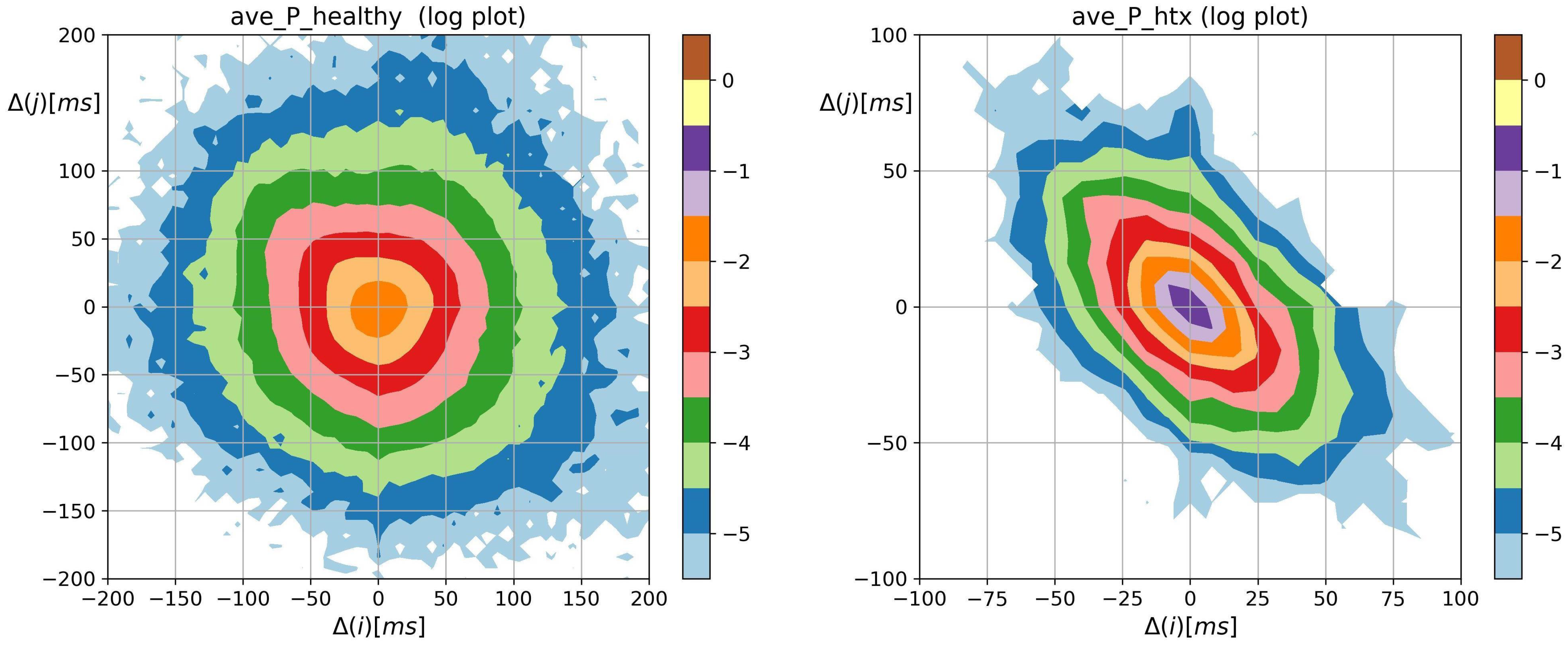
Figure 2 shows the means of probability matrices P , where two events, i.e., Δ i and then Δ j , may occur sequentially in a typical signal of RR increments belonging to the group consisting of a healthy person and a HTX patient. First of all, the difference in the spread of events: from −200 ms to 200 ms in the case of healthy individuals, to −100 ms to 100 ms in the case of HTX patients, should be noted. Moreover, the shape of P for healthy persons is similar to a shooting target (in the logarithmic scale) centered around ( 0 , 0 ) . Matrix P of HTX patients resembles an ellipse with a sharp vertex, centered at ( 0 , 0 ) . The short axes of this ellipse coincide with the identity line; the longer axes are perpendicular to the short ones and coincide with the second diagonal of the XY-plane.
The most probable two-element pattern in P is ( 0 , 0 ) for both groups. However, the mean probability of that event differs much. Its value is about 0.029 ± 0.04 in the case of the group of healthy people and about 0.223 ± 0.013 in the case of HTX recipients ( 0.194 ± 0.075 for the NG group, 0.238 ± 0.013 for the CR group, and 0.222 ± 0.027 for the H group, see the appendix for details). The prevailing two-element patterns, the core patterns, are built of symbols { 16 , 8 , 0 , + 8 , + 16 } in the case of HTX patients. The total probabilities of observing the events in that group were 0.91 ± 0.10 in the NG group signals, 0.96 ± 0.09 in the CR group signals, and 0.95 ± 0.20 in the H group signals. In the case of healthy people, the probability greater than 0.92 ± 0.05 was observed for the events represented by the following symbols { 72 , , 8 , 0 , + 8 , , + 72 } .
Moreover, the dynamics of the heart rate in patients after HTX is asymmetric. Namely, the probabilities of two subsequent accelerations or decelerations of a given size Δ > 0 , i.e., points of ( Δ , Δ ) , ( + Δ , + Δ ) in P matrix and alternating patterns of acceleration and deceleration of this size: ( Δ , + Δ ) , ( + Δ , Δ ) are rather similar to each other in the case of healthy people but they are significantly different for HTX patients. The specificity of this asymmetry can be learned from probabilities of two subsequent accelerations or decelerations of size 24, i.e., ( 24 , 24 ) , ( + 24 , + 24 ) and alternating patterns of acceleration and deceleration of this size: ( 24 , + 24 ) , ( + 24 , 24 ) in the studied groups, namely:
pattern healthy N G C R H ( 24 , 24 ) ( 4.6 ± 2.1 ) 10 3 ( 4.7 ± 4.1 ) 10 5 ( 3.7 ± 1.8 ) 10 5 ( 5.8 ± 5.4 ) 10 6 ( 24 , + 24 ) ( 5.3 ± 3.2 ) 10 3 ( 4.3 ± 2.0 ) 10 3 ( 8.8 ± 1.7 ) 10 4 ( 1.4 ± 0.5 ) 10 4 ( + 24 , 24 ) ( 4.3 ± 2.4 ) 10 3 ( 4.8 ± 2.0 ) 10 3 ( 1.7 ± 0.6 ) 10 3 ( 1.8 ± 0.8 ) 10 3 ( + 24 , + 24 ) ( 4.5 ± 2.6 ) 10 3 ( 5.5 ± 3.8 ) 10 5 ( 3.1 ± 1.6 ) 10 5 ( 5.6 ± 5.4 ) 10 6
In the case of HTX patients, when Δ = 24 ms, the alternating patterns are present and about 100 times more likely than monotonic patterns. This feature is not present in the heart rhythms of healthy coevals.
The overall shape of the distribution of Shannon entropy of two-element RR increment patterns resembles the spread and shapes of the probability matrices P shown in Figure 2. However, the steepness of the core dynamics, by which we mean events when Δ 50 , is weakened, which enhances visualization of dynamical asymmetry in signals of HTX patients. Bearing in mind the different scales used in Figure 3, one can observe the large variability of events in the case of healthy individuals and their restriction in the case of signals from HTX patients. This feature is evidently demonstrated in matrices of transition probabilities T , see Figure 4.
From Figure 4, we see the distribution of the following events after a given event occurs. The most probable transition, given a system performed 0 RR increment, is the 0 transition, i.e., a transition 0 0 takes place. Its mean probability was greater than 0.5 in the case of heart rhythms of HTX recipients and about 0.17 in the group of healthy coevals. The probabilities of transitions in signals of HTX patients emphasized that the studied dynamics not only prefer alternating patterns but is of the damped type: after any acceleration, it is more likely to see a deceleration of the smaller size than other event and vice versa, after any deceleration it is more likely to observe an acceleration of a smaller size. This property is absent in the core dynamics of heart rhythms of healthy individuals. Therefore, in the case of HTX patients, the main shape of the matrix T in Figure 4 is arranged along half of the anti-identity line on XY-plane ( y = 1 2 x ), while in the case of healthy people, this main shape appears to be insensitive to whether there was acceleration or deceleration.
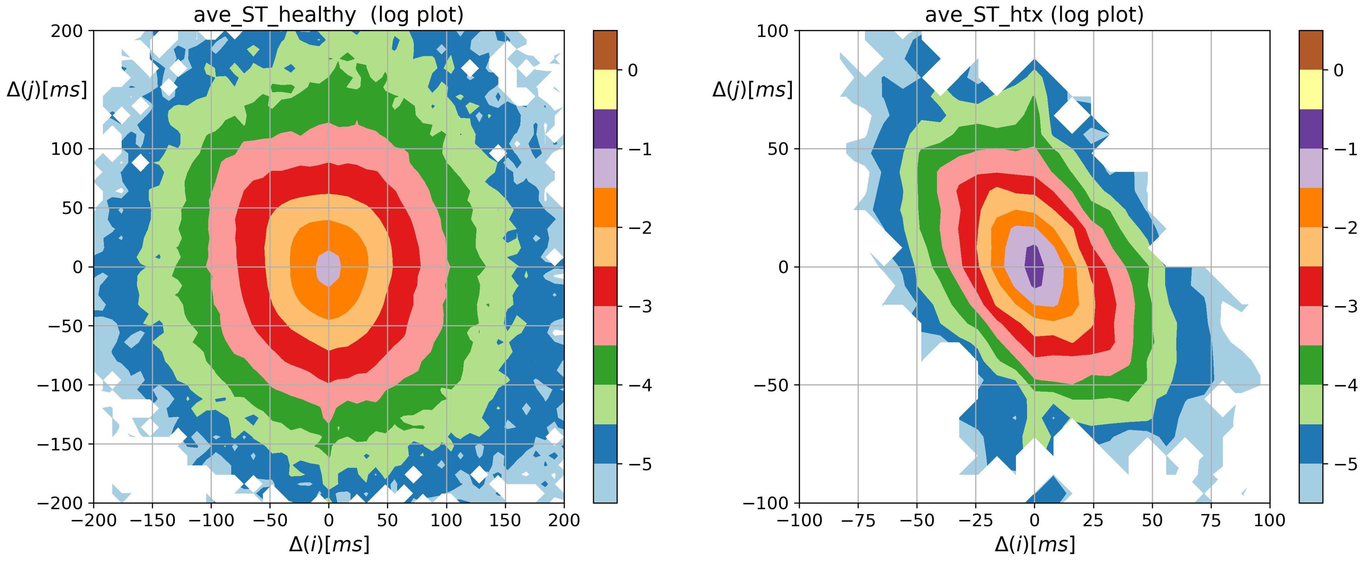
The two-point distribution of the transition rates S _ T shown in Figure 5, is the distribution of the probability matrix P entries modulated by the logarithms of transition matrix T elements. One can observe the switch in the dynamics after a 0 event in the heart rate dynamics of HTX patients. Now, the peaks of the transition rates concentrate on ( 0 , 0 ) , ( 0 , + 8 ) and ( 0 , 8 ) indicating their non-Markovian origin.
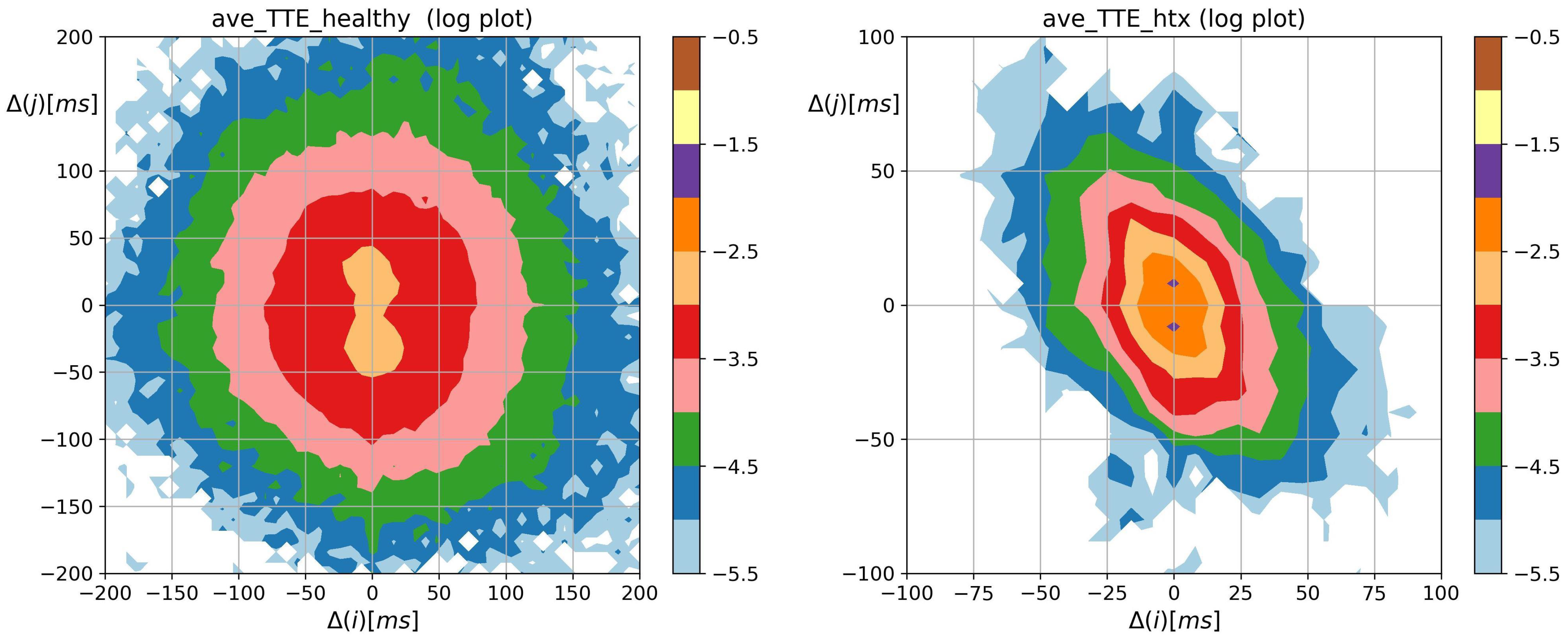
Figure 6 argues that the strongest memory effects are revealed at small-magnitude transitions. Namely, in the case of healthy individuals, the memories of past events are related to events after acceleration or deceleration that is smaller than 20 ms, and there is a change of a larger size. In the case of the heart rhythm after a HTX, the strongest memory effect is visible in the case of transitions 0 ± 8 .

3.3. Segmented Signal HRV Analysis

All segments consisting of 21 to 450 points were found numerically stable in our estimates. However, the statistical analysis of the p N N 50 segment values occurred unreliable due to the dominance of the zero value. Therefore our considerations omit reporting properties obtained for the p N N 50 in segments.
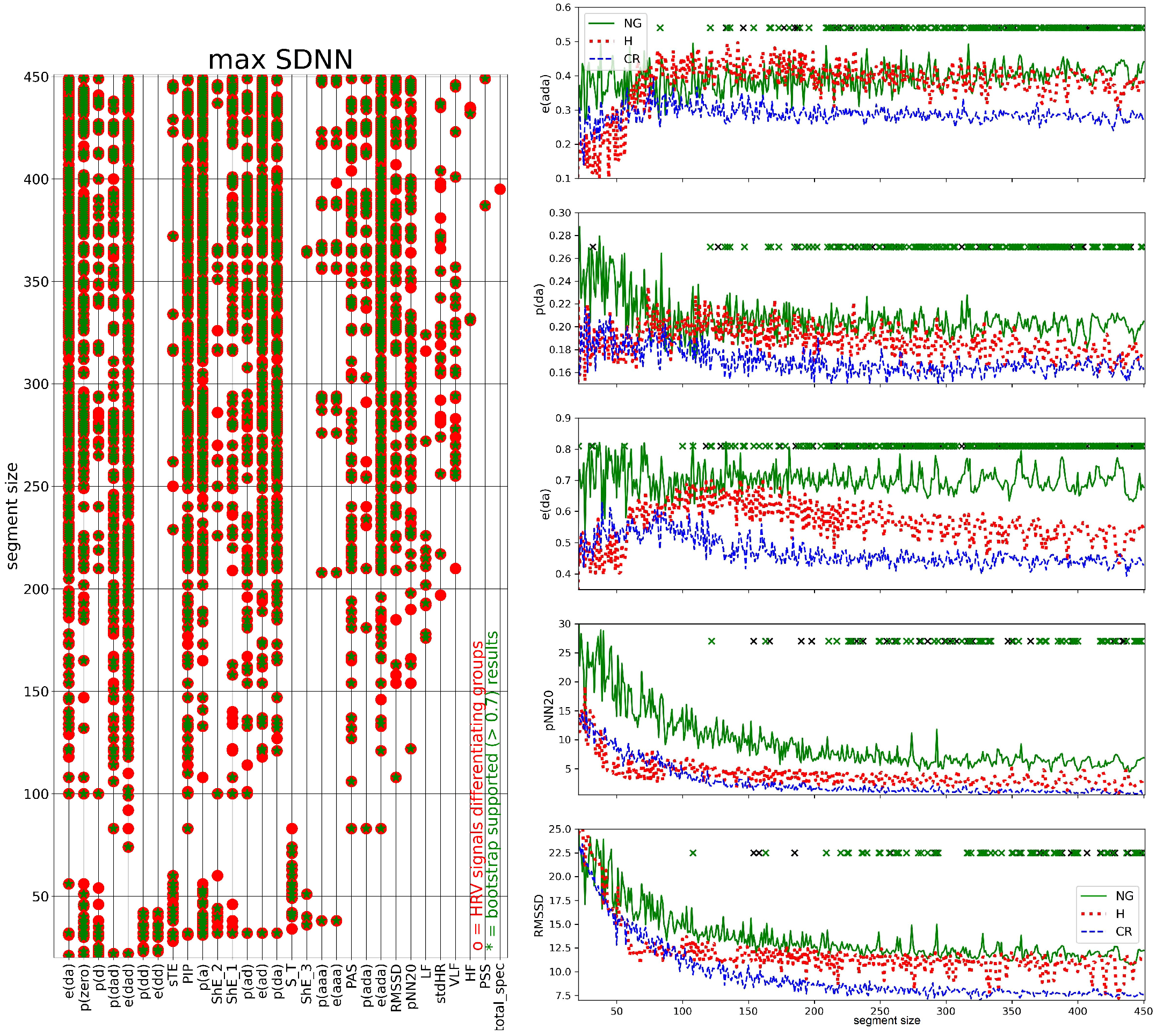
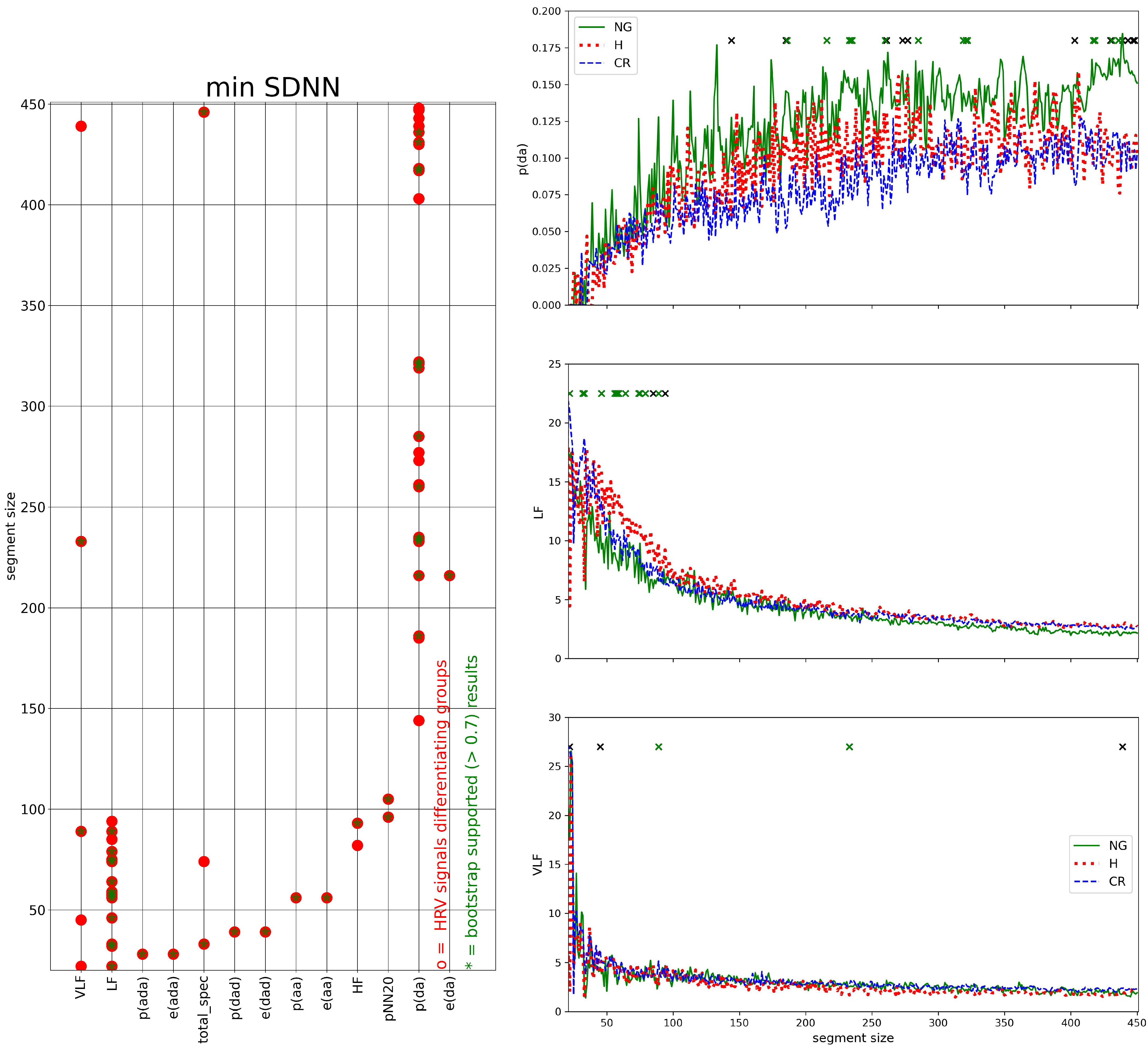
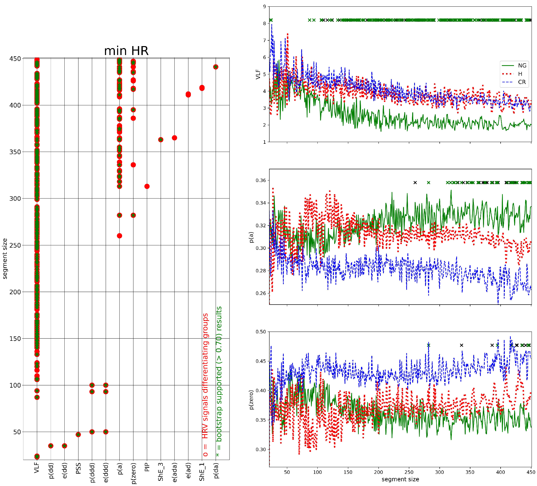
In Figure 7, Figure 8, Figure 9 and Figure 10, we show the results of the I-type analysis of the segmented series of HRV, see Section 2.7. The HRV analysis was carried out in one segment extracted from each HRV series: the segment with the maximal SDNN (Figure 7), minimal SDNN (Figure 8), maximal HR (Figure 9), and minimal HR (Figure 10). The plots in the left columns of these Figs display the names of measures against the segment size for which the statistically significant difference between the groups was found. On the right-hand columns of these figures, there are dependencies of the most important HRV measures in the segment sizes, namely there are plots of measures that provide the largest number of segments differentiating the studied groups, differentiated in five segments. Such measures were considered as candidates for group discriminators.
Windows characterized by the maximal SDNN provided the largest set of HRV measures (thirty) differentiating the studied groups; see Figure 7 on the left. For all studied HRV measures, except meanRR and meanHR, there were window sizes s which differentiated the groups. Among them, there were measures that successfully differentiated the groups in small window sizes only, namely when s < 100 : p(dd), e(dd), sTE, and S_T, contrary to measures pNN20, LF, HF, or RMSSD, which found group differences only in large window sizes, i.e., when s 100 .
The largest numbers of window sizes that were successful in group differentiation were obtained for e(ada): 173, p(da): 160, e(da): 156, pNN20: 82 and RMSSD: 80, see plots of the group medians of these HRV measures versus segment size in Figure 7 on the right. For almost all segment sizes, these results were supported by more than 70% simulations of the bootstrap test. The plots show that for the window size s > 300 the values of HRV measures stabilized. The visible variations around the stable values were due to the fact that the median group values were plotted. Those stable values obtained from the CR group attained the lowest values among the studied groups. It is evident for e C R (ada) < e not C R (ada), e C R (da) < e not C R (da), and RMSSD C R < RMSSD not C R . In the same segment size region, signals representing the NG group reached the highest values, see, e.g., p N G (da) > p not N G (da) and e N G (da) > e not N G (da).
From the comparison of plots of p(da) and e(da) in Figure 7 on the right we see that variability of d a events quantified by entropy better differentiated studied groups than simple counters of these events as the separation between the stable group values is more evident when the segment sizes were large. The CR group was distinguished by stabilization at the lowest values—half of the NG group. There is a switch in the relations between the group stable values when one moves from the small-sized windows to the large-sized windows.
In contrast, the windows in which the signals were characterized by the smallest SDNN values, provided only eleven measures that detected significant differences between the studied groups, see Figure 8. At most, they were related to the power spectrum. However, the p(da) measure gave the largest number of window sizes, i.e., 25, which differentiated the groups. The frequency measures differentiated groups for small window sizes only, and those statistical findings had rather low support from the bootstrap test. As s increased, all group medians stabilized rather fast and at small values. At most, the successes in group differentiation were achieved in small-sized segments. In segments of size 50 < s < 100 , the values L F obtained from the group H signals were greater than in the rest of the group signals, i.e., LF H > LF not H , which can be useful in clinical practice.
In the case of windows corresponding to the largest HR for a given window size, see Figure 9, we obtained thirty HRV measures differentiating the studied groups. The measures which differentiated in the largest number of segment sizes were e(ad): 112, e(da): 75, e(ada): 73, ShE_1: 44 and sTE: 33. All of them were entropic type measures. Thus, the segments with the highest HR would indicate that the groups were different due to the variability of events rather than by the number of events. The highest values of these measures were attained on signals of the NG group for large segment sizes.
It is worth it to compare the plots of e(da) obtained from segments with max SDNN (Figure 7) to those obtained from segments with max HR (Figure 9) to learn how the complexity of the signals changed when the organism was exposed to different challenges. Although the relationships between the stable group values are similar in both figures, the stable values are different, i.e., lower in the cases of maximum HR segments.
The results, provided by windows where the minimal HR was observed (Figure 10), pointed at VLF as the measure which best differentiated the studied groups. The VLF differentiated the groups into 209 segment sizes, and almost all of those results were supported in the bootstrap test. Stable values of VLF obtained for the NG group were significantly the smallest, VLF N G < VLF not N G , which can be used in clinical practice. The p(a) was the next measure differentiating the groups in the case of min HR. That measure found groups different in 55 segment sizes, all of them were of sizes greater than 250. The third plot in Figure 10 on the right is related to p(zero); the group distinction was statistically significant in 14 segments of large sizes. The highest values of p(zero) were found for signals of the CR group.
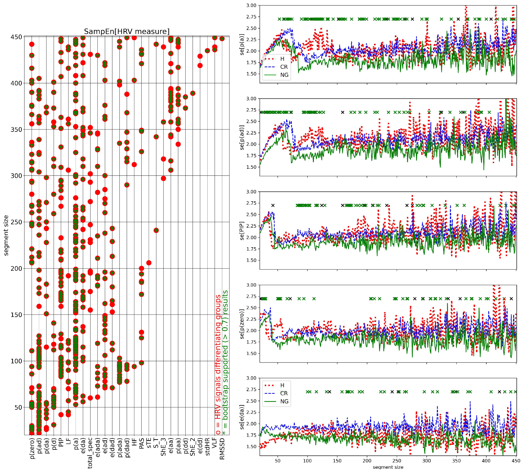
The complexity of the entire series of the segmented HRV values was evaluated by the std of all values of a given HRV measure obtained in subsequent windows, and by the SampEn of these values. In Figure 11, the results obtained for std are shown, in Figure 12, the results obtained for SampEn are presented.
In the case of value variation estimated by std, Figure 11, the strongest group differentiation was observed for e(ad): 71 segment sizes. However, only 31 were supported by the bootstrap test. The obtained values of std[e(ad)] in different segment sizes showed a stable relationship between the groups: std[e(ad) N G ] > std[e(ad) not N G ] and std[e(ad) C R ] < std[e(ad) not C R ]. The std[e(ada)] provided a group differentiation in 47 segment sizes, all of them were of size greater than about 40 and smaller than about 200 RR intervals. Moreover, the signals of the H group stabilized in that segment size range, at the highest values, i.e., std[e(ada) H ] > std[e(ada) not H ], which could be clinically useful.
The remaining plots in Figure 11 on the right, std[e(dad)] and std[VLF], revealed group differences for 17 and 16 segment sizes, respectively. All of those segments were smaller than 150. For the segment sizes, both plots demonstrate a stable relationship between the variability of measures: std[e(dad) C R ] < std[e(dad) not C R ] and std[VLF N G ] < std[VLF not N G ].
The relationship between subsequent values in HRV series in segmented HRV series, evaluated by SampEn, gave the group differentiation for many of the investigated measures. The greatest number of segment sizes differentiating the groups were observed for the following HRV series: SampEn[p(a)]: 87, SampEn[p(ad)]: 71, SampEn[PIP]: 55, SampEn[p(zero)]: 49, and SampEn[e(da)]: 36, see Figure 12 on the left for the whole list. These window sizes were scattered over the studied range of window sizes, which could indicate that observed relations were driven by some other processes of physiological origin where the intensity changed in time.
The dependence of SampEn of listed above measures on the segment size showed that in segments of small sizes, s < 150 (which lasts for less than 100 seconds) SampEn displayed distinct relationships between the subsequent segment values than values obtained when segments were larger than 200 points. After steady increases in SampEn values when the segment size increased, there were observed rapid jumps down to low values. Such jumps from high to low values of SampEn might indicate switching on of the oscillatory processes which activity corresponded to 30 to 100 s. The switches took place at distinct segment sizes when different groups and different HRV measures were investigated.
Moreover, for large segment sizes, the high values of SampEn were attained by signals of the H group, indicating the highest unpredictability in values of segmented HRV measures. On the other hand, the median of the NG group was the smallest among the medians of the groups studied indicating the highest predictability in segmented HRV signals which might be the effect of the strength of control processes.

4. Discussion and Summary

The HRV may encompass not only autonomic modulation but also variability from abnormal heart rate patterns—irregular sinus arrhythmia of non-respiratory origin, referred to as erratic rhythm [3,15]. The erratic rhythm has been attributed to higher HRV scores observed in elderly people, especially among short-term HRV indices [38,66]. Because of alternations in electrogenic transport processes within the cardiac myocytes, LVH affects the electrophysiological remodeling of cardiac tissue, leading to an increased risk of malignant arrhythmia [67].
To observe abnormalities in heart rhythm events, long time series are required. In order to obtain reliable long signals, where the effects of editing were reduced as much as possible, we decided to limit ourselves to nocturnal recordings. Sleep is assumed as an excellent time to measure the autonomic regulatory functions because sleep is organized in cycles of autonomic regulation activity [66,68]. Each cycle lasts about 90 min, where stages of slow wave sleep (non-rapid eye movement sleep NREM) are followed by rapid eye movement sleep (REM) [69]. It has been recognized that NREM sleep is characterized by vagal drive while the REM stage exhibits elevated sympathetic modulation and a loss of vagal control. Therefore, while investigating nocturnal series, one must expect to observe transformations in autonomic function caused by switches between different states of sleep [27,42,66,68,70].
Thanks to the symbolic representation of accelerations and decelerations, our method allowed for the direct usage of nonlinear analysis tools aimed at the dynamics quantification of the RR interval time series. In particular, tools based on the presence of acceleration and deceleration in alternating patterns proved effective at distinguishing between the studied groups. Our results showed that in HTX patients shortly after the surgery, the LVH influence can be observed through HRV. Equipped with the results of the HRV analysis, we can follow the development of LVH, i.e., whether LVH is associated with an increase in RWT (the case of the CR group) or whether LVH is associated with an increase in LVM (the case of the H group).
The standard estimates were obtained from the whole signals; hence, such a cumulative outlook at all recorded events did not find any linear measure of HRV that would distinguish between patient signals from different groups. Only p(da), counting the occurrences of the d a pattern, statistically significantly differentiated the signals from the NG group from the signals of the CR group. To obtain deeper insight into the variety of events summarized by the total outlook, we propose the efficient visualization of the distribution of some relevant features. These distributions defined on two-element patterns of RR increments could be friendly reported in a form similar to the well-known 3D Poincare plots, the graphs appreciated by cardiologists. With this technique, key components and crucial characteristics of the heart rate dynamics can be detected and/or emphasized.
In particular, P matrices of the probability of the two-element patterns and T matrices of transitions between two element patterns provided the following aspects of the stochastic dynamics of the heart rhythm contractions in patients after HTX when compared to the healthy coevals:
  • The probability distribution P of HTX patients was strongly steep, and sharply peaked at pattern ( 00 ) m where the basic transitions involving accelerations and/or decelerations of magnitude 16 covered more than 90%.
  • Accelerations and decelerations were likely to occur alternately, which affected RR intervals (i.e., to change the mean value in a pendulum-type motion rather than as a stochastic walk). Alternating patterns were observed 100 times more frequently than monotonic patterns. This pendulum-type motion was damped in HTX patients.
  • Similar to the healthy coevals, the strongest memory effects in patients after HTX were associated with transitions opposite to damped alternating dynamics.
The segmented HRV, i.e., series of HRV values obtained from splitting the entire signal into windows of equal size (equal in the number of RR intervals), allowed us to study the instantaneous properties of the heart rate. Different aspects of heart rate dynamics can be studied with a windowed approach due to exploration concentrated on selected segments of signals directly related to events of interest. In the following, we investigated alternations in HR due to autonomic activity or abnormal rhythms. We decided to study windows of size 21 to 450 RR intervals to avoid numerical problems in estimates of frequency measures and instabilities resulting from counting rare events.
Increases in heart rate reflect decreased vagal and/or increased sympathetic control of heart rate. Therefore, we proposed to study HRV in windows characterized by the maximal HR to observe the REM parts of the nocturnal rest, and in segments with minimal HR which should refer to the slow-wave sleep [66,68]. As REM sleep typically lasts 10 min or longer, windows with a large number of RR intervals may be representative of testing HRV during REM sleep.
We have found that, when the window size was large enough, the segments representing the maximal HR differentiated the signals of the studied groups by the entropy of a d and d a events. The NG group displayed higher complexity than the signals of other groups, especially compared to the signals of the CR group. Thus sympathetic activity influence on heart rate occurred more irregularly and was richer in a variety of events in patient signals from the NG group. The vagal impact, best described by VLF in segments with minimal HR, also indicated another key difference between the groups. The VLF values obtained by signals of the NG group occurred significantly lower than in signals of other groups. However, the power in V L F is known to encompass most sleep-disordered breathing and periodic limb movements [66]. It is also known that during NREM sleep, arousal fluctuations appear with pseudo-rhythmic modality, recurring about 20–40 s [44,71], i.e., in periods where power is estimated by V L F . Having no information on breathing problems or periodic limb movements in our patients, we can only speculate that these events were less likely in the NG patients.
To meet the mathematical demand of stationarity, the segments of 250 and 300 beats with minimal SDNN are commonly selected from longer RR interval signals [34,44,47]. They are considered to be representatives of the basic tone of autonomic heart rate regulation. In the case of the minimal SDNN segments extracted from our series, we did not observe statistically satisfactory differences between the groups for any segment size. However, the segments with the highest SDNN proved group differences in many aspects. The linear and nonlinear HRV measures gave high variability /complexity of signals from the NG group and the lowest variability in signals from the CR group. The high SDNN value might represent moments of irregular events, and possible erratic rhythms. However, also the moments of high variability may result from the stronger response to the actual organism needs, which in the case of the CR group may be impaired.
The set of momentary HRV values was evaluated by std provided the greatest variety among the entropies of a d and a d a patterns. Compiling together the characteristics of e(ada) obtained from the window with maximal SDNN with the variability of e(ada), i.e., std[e(ada)], we discovered a tool that could be efficient in distinguishing the geometry of the CR heart from the heart geometry of the H group because the highest values in std[e(ada)] were achieved by signals from the H group for scales s between 50 and 100 heartbeats.
The relationship between the consecutive elements of the momentary HRV series, evaluated by SampEn, showed that the frequency of a and a d patterns in signals of the NG group displayed the highest predictability, while in signals of the H group—they were the most unpredictable. In particular, this observation concerned window sizes from 100 to 150 RR intervals.
Finally, the limitations of our findings must be enumerated. First, the presented method was effective in discerning LVH but the results were based on a rather small groups of patients. Second, the method was only applied to the signals of HTX patients. Therefore, its usefulness in the case of RR interval signals coming from the general population is unknown. However, since this method revealed the emergence of irregular rhythms in the elderly [46], we can hypothesize that it should be effective. Third, due to the resolution of our Holter recordings, the symbolization applied to RR increments was based on Δ 0 = 8 ms. Such symbolization is enough to observe sympathetic stimulation and to filter out possible noise effects well. However, tests in which the method uses a smaller symbolization interval Δ 0 could further justify our findings.

5. Conclusions

Entropic measures are among the most frequently used methods of quantification of the complexity in a time series [53]. Based on the Shannon entropy conception of the unpredictability of a given event, entropy measures express our intuitive understanding of regularity (low unpredictability) or irregularity (high unpredictability) in a time series. Low unpredictability makes sense of the deterministic modeling of the source of a signal, which in the case of RR intervals supports modeling baroreflex oscillations [72,73,74]. Therefore, pattern counters and entropic measures have been widely used in many studies on the complexity of RR intervals; see [30,37]. However, nonlinear measures neither estimate the magnitude of variability nor reflect specific components of autonomic modulation (but they quantify the complexity of RR interval time series).
A simple idea for detecting anomalies in a time series is to observe the typical behaviors of the time series and compare them to other data. Our signals, consisting of 20,000 RR intervals of nocturnal rest, were nonstationary and, hence, represent the whole set of complex phenomena (not only from autonomic regulation). The alterations in the nocturnal rhythm of heartbeats, first of all, may be associated with transitions in the sleep cycle. However, then the appearance of abnormal heart rhythms may strongly modify the heart rhythm [42,66,68]. Finally, the increased HRV may result from the signal preprocessing, called the scanning error: uneven beat detection, missed, or misclassified beats [66]. All of them could have confounding effects on HRV analysis. Segmenting a signal into small windows allowed us to search for the moments of special interest. This systematic exploration of the time-dependent aspects of RR intervals shows that our approach should be appreciated when the question arises of whether elevated HRV is due to autonomic regulation, irregular heart rhythm patterns, a preprocessing signal, or another unknown reason.
Combined together, we can claim that in HTX patients, shortly after the surgery, the LVH can be observed through HRV. We found that some HRV measures show statistically significant relationships more often with windows containing few RR intervals, while others frequently differentiate studied groups only when the window size is larger. However, we could not determine the perfect window size, possibly due to including too few signals, resulting in weaker coherence and ambiguous results. Despite this, we could use the segmented series to follow LVH development and recognize associated increases in RWT or LVM. The main limitation was the small sample size, so further investigation is needed to confirm our findings.
In our dynamic patterns study, we used the Kruskal–Wallis test with bootstrap modifications to differentiate groups, but incorporating ML methods, such as classification, clustering, and factor analysis, could shed new light on the observed pattern variability. Therefore, we plan to explore ML methods in further development.
To increase the clinical utility of our method, we can select a window for studying signal properties based on specific purposes, e.g., windows with maximum/minimum LF or HF can estimate the baroreceptor performance. We plan to investigate changes in autonomic regulation caused by biological aging using this approach.

Author Contributions

Conception and clinical data collection: J.W.; invented the RR increment analysis: D.M.; writing—review and editing: J.W. and D.M.; visualization: D.M.; supervision: M.G. All authors approved the final manuscript as submitted, and agreed to be accountable for all aspects of the work. All authors have read and agreed to the published version of the manuscript.

Funding

This research received no external funding.

Institutional Review Board Statement

The study was conducted in accordance with Declaration of Helsinki, and approved by the Independent Bioethics Committee for Scientific Research at the Medical University of Gdańsk (protocol code NKBBN/142-58/2023 issued on 2 February 2023).

Informed Consent Statement

All procedures performed in the study were in accordance with the ethical standards approved by the Bioethics Commission for Research of the Medical University of Gdansk with the 1964 Helsinki Declaration and its later amendments. Informed consent was obtained from all individuals participating in the study during admission to the hospital.

Data Availability Statement

The studied RR interval signals of HTX patients are available upon request to D.M.

Acknowledgments

We thank Maciej Duda of the Department of Cardiac and Vascular Surgery of the Medical University of Gdansk for help with the patients’ data acquisition.

Conflicts of Interest

The authors declare that the research was conducted in the absence of any commercial or financial relationships that could be construed as a potential conflict of interest.

Appendix A

In Figure A1, we show the means of probability matrices P , where two events, i.e., Δ i and then Δ j , may occur sequentially in a typical RR increment signal belonging to the HTX patient group.
We should note that P takes an ellipse-type shape centered at ( 0 , 0 ) , with short axes coinciding with the identity line and longer axes, perpendicular to the short ones, coinciding with the second diagonal of the XY-plane. The plots seem to be symmetrical with respect to the long axis. Regarding the shorter axis, symmetry is less evident, especially in the case of the CR group.
Figure A1. The contour plots of probability (in the logarithmic scale) to meet an event: Δ i followed by Δ j , obtained from signals of RR intervals pooled in groups NG, H, and CR. Δ means the magnitude in ms of a deceleration, Δ > 0 , or acceleration, Δ < 0 .
Biomedinformatics 03 00015 g0a1
The most probable 2-element pattern in P was ( 0 , 0 ) for all groups. The mean probability of that event was 0.194 ± 0.075 for the NG group, 0.238 ± 0.013 for the CR group, and 0.222 ± 0.027 for the H group. The prevailing 2-element patterns, i.e., the core patterns, were made of symbols { 16 , 8 , 0 , + 8 , + 16 } . The total probabilities of observing the events of the groups were 0.91 ± 0.10 in the NG group signals, 0.96 ± 0.09 in the CR group signals, and 0.95 ± 0.20 in the H group signals, which indicate that the signals of the CR and H groups exhibited more restricted basic rhythms compared to the signals of the NG group. The specificity of the asymmetry in the dynamics of the HTX patient is described in (12), showing that alternating patterns occur many times (and are more likely than monotonic patterns).
Figure A2. The contour plots of probability of the transition Δ i Δ j  while being in Δ i , obtained from signals of RR increments pooled in groups NG, H, and CR. Δ means the magnitude in ms of a deceleration, Δ > 0 , or acceleration, Δ < 0 .
Biomedinformatics 03 00015 g0a2
The results discussed in Section 3.1 show that the probabilities of all patterns of the type d i a j (the sum over the right-bottom quadrant in Figure A1) differentiate statistically from the studied groups. In Figure A1, this quadrant is less occupied in the CR group than in the other groups.
In Figure A2, the matrices of the group means of transition probabilities between RR increments are shown. The most probable transition, given a system performed the 0 RR increment, was to 0, i.e., 0 0 . Its mean probability was 0.502 ± 0.033 for the NG group signals, 0.545 ± 0.016 for the CR group signals, and 0.518 ± 0.040 for H group signals. The probabilities of other transitions from the core patterns emphasized that the examined dynamics were of the damped bell type. After an acceleration, one would more likely see a deceleration of the smaller size than other events and vice versa; after a deceleration, one would more likely observe an acceleration of a smaller size. For example, regarding the considered signals, the most likely transitions after events 16 and + 16 were as follows:
transition N G C R H 16 + 24 0.107 ± 0.034 0.035 ± 0.008 0.051 ± 0.020 16 + 16 0.222 ± 0.035 0.191 ± 0.025 0.220 ± 0.050 16 + 8 0.367 ± 0.034 0.487 ± 0.040 0.410 ± 0.083 16 0 0.200 ± 0.029 0.205 ± 0.022 0.229 ± 0.041 16 8 0.060 ± 0.017 0.047 ± 0.015 0.047 ± 0.016 16 16 0.013 ± 0.004 0.011 ± 0.004 0.012 ± 0.004 16 24 0.004 ± 0.003 0.003 ± 0.001 0.004 ± 0.001 + 16 + 24 0.004 ± 0.002 0.004 ± 0.002 0.001 ± 0.001 + 16 + 16 0.012 ± 0.004 0.014 ± 0.005 0.016 ± 0.006 + 16 + 8 0.043 ± 0.010 0.029 ± 0.010 0.038 ± 0.014 + 16 0 0.161 ± 0.025 0.141 ± 0.017 0.185 ± 0.044 + 16 8 0.423 ± 0.032 0.052 ± 0.042 0.382 ± 0.070 + 16 16 0.271 ± 0.035 0.255 ± 0.024 0.316 ± 0.056 + 16 24 0.066 ± 0.012 0.039 ± 0.009 0.045 ± 0.017
Thus, the transitions 16 + 8 and + 16 8 were significantly more probable than the other ones. Therefore, the main shapes of the matrices T in Figure A2 were arranged along half of the anti-identity line on the XY-plane ( y = 1 2 x ). From (A1), we see that such an arrangement occurred in the most fixed signals from the CR group.
The other differences between the group dynamics became apparent when signals corresponded to extreme situations, to events that were far from typical ones. For example, in Figure A2, one may compare the diversity in the transition distributions after RR increments of a magnitude that is 48 ms or greater. The H group displayed the greatest variability here.
To complete the presentation of the visualization method, in Figure A3, Figure A4 and Figure A5, the contour plots of entropic matrices E , S _ T , and TTE , respectively, are shown.
The overall shape of the distribution of the Shannon entropy of two-element RR increment patterns reflects the shape of the probability matrix P shown in Figure A1. However, the steepness of the base part that represents the core dynamics (i.e., when Δ 16 ) is weakened.
The two-point distribution of the transition rates S _ T shown in Figure A4, following Equation (10), is the distribution of the probability matrix P entries modulated by the logarithms of transition matrix T elements.
From Figure A5, we learn that the strongest memory effect revealed for 0 ± 8 is independent of the HTX group.
Figure A3. The contour plots of the Shannon entropy matrix S h E _ 2 for probability distribution to meet an event: Δ i followed by Δ j . Results were obtained from signals of RR intervals pooled in groups NG, H, and CR. Δ means the magnitude in ms of a deceleration, Δ > 0 , or acceleration, Δ < 0 .
Biomedinformatics 03 00015 g0a3
Figure A4. The contour plots of the entropy of transition rate matrix S _ T quantifying Markovian dynamics for an event, i.e., Δ i followed by Δ j . Results were obtained from signals of RR intervals pooled in groups NG, H, and CR. Δ means the magnitude in ms of a deceleration, Δ > 0 , or acceleration, Δ < 0 .
Biomedinformatics 03 00015 g0a4
Figure A5. The contour plots of matrix TTE quantifying the memory effects in probability to observe a sequence of events, i.e., Δ i followed by Δ j . Results were obtained from signals of RR intervals pooled in groups NG, H, and CR. Δ means the magnitude in ms of a deceleration, Δ > 0 , or acceleration, Δ < 0 .
Biomedinformatics 03 00015 g0a5

References

  1. Malik, M.; Bigger, J.T.; Camm, A.J.; Kleiger, R.E.; Malliani, A.; Moss, A.J.; Schwartz, P.J. Heart rate variability: Standards of measurement, physiological interpretation, and clinical use. Eur. Heart J. 1996, 17, 354–381. [Google Scholar] [CrossRef] [Green Version]
  2. Goldberger, A.L.; Stein, P.K. Evaluation of Heart Rate Variability. 2020. Available online: http://www.uptodate.com/contents/evaluation-of-heart-rate-variability (accessed on 29 December 2022).
  3. Shaffer, F.; Ginberg, J. An Overview of Heart Rate Variability Metrics and Norms. Front. Public Health 2017, 5, 258. [Google Scholar] [CrossRef] [PubMed] [Green Version]
  4. Saul, J.P.; Valenza, G. Heart rate variability and the dawn of complex physiological signal analysis: Methodological and clinical perspectives. Philos. Trans. R. Soc. A Math. Phys. Eng. Sci. 2021, 379, 20200255. [Google Scholar] [CrossRef] [PubMed]
  5. Pikkujämsä, S.M.; Mäkikallio, T.H.; Sourander, L.B.; Räihä, I.J.; Puukka, P.; Skyttä, J.; Peng, C.K.; Goldberger, A.L.; Huikuri, H.V. Cardiac interbeat interval dynamics from childhood to senescence: Comparison of conventional and new measures based on fractals and chaos theory. Circulation 1999, 100, 393–399. [Google Scholar] [CrossRef] [Green Version]
  6. Meersman, R.E.D.; Stein, P.K. Vagal modulation and aging. Biol. Psychol. 2007, 74, 165–173. [Google Scholar] [CrossRef]
  7. Tsuji, H.; Larson, M.G.; Venditti, F.J.; Manders, E.S.; Evans, J.C.; Feldman, C.L.; Levy, D. Impact of Reduced Heart Rate Variability on Risk for Cardiac Events. Circulation 1996, 94, 2850–2855. [Google Scholar] [CrossRef] [Green Version]
  8. Nolan, J.; Batin, P.D.; Andrews, R.; Lindsay, S.J.; Brooksby, P.; Mullen, M.; Baig, W.; Flapan, A.D.; Cowley, A.; Prescott, R.J.; et al. Prospective Study of Heart Rate Variability and Mortality in Chronic Heart Failure. Circulation 1998, 98, 1510–1516. [Google Scholar] [CrossRef] [Green Version]
  9. Huikuri, H.V.; Stein, P.K. Heart Rate Variability in Risk Stratification of Cardiac Patients. Prog. Cardiovasc. Dis. 2013, 56, 153–159. [Google Scholar] [CrossRef]
  10. Alter, P.; Grimm, W.; Vollrath, A.; Czerny, F.; Maisch, B. Heart rate variability in patients with cardiac hypertrophy—Relation to left ventricular mass and etiology. Am. Heart J. 2006, 151, 829–836. [Google Scholar] [CrossRef]
  11. Vuoti, A.O.; Tulppo, M.P.; Ukkola, O.H.; Junttila, M.J.; Huikuri, H.V.; Kiviniemi, A.M.; Perkiömäki, J.S. Prognostic value of heart rate variability in patients with coronary artery disease in the current treatment era. PLoS ONE 2021, 16, e0254107. [Google Scholar] [CrossRef]
  12. Thayer, J.F.; Yamamoto, S.S.; Brosschot, J.F. The relationship of autonomic imbalance, heart rate variability and cardiovascular disease risk factors. Int. J. Cardiol. 2010, 141, 122–131. [Google Scholar] [CrossRef] [PubMed]
  13. Tracy, E.; Rowe, G.; LeBlanc, A.J. Cardiac tissue remodeling in healthy aging: The road to pathology. Am. J.-Physiol.-Cell Physiol. 2020, 319, C166–C182. [Google Scholar] [CrossRef] [PubMed]
  14. Frantz, S.; Hundertmark, M.J.; Schulz-Menger, J.; Bengel, F.M.; Bauersachs, J. Left ventricular remodelling post-myocardial infarction: Pathophysiology, imaging, and novel therapies. Eur. Heart J. 2022, 43, 2549–2561. [Google Scholar] [CrossRef] [PubMed]
  15. Stein, P.K.; Le, Q.; Domitrovich, P.P. Development of more erratic heart rate patterns is associated with mortality post-myocardial infarction. J. Electrocardiol. 2008, 41, 110–115. [Google Scholar] [CrossRef] [Green Version]
  16. Lang, R.M.; Badano, L.P.; Mor-Avi, V.; Afilalo, J.; Armstrong, A.; Ernande, L.; Flachskampf, F.A.; Foster, E.; Goldstein, S.A.; Kuznetsova, T.; et al. Recommendations for Cardiac Chamber Quantification by Echocardiography in Adults: An Update from the American Society of Echocardiography and the European Association of Cardiovascular Imaging. Eur. Heart J.-Cardiovasc. Imaging 2015, 16, 233–271. [Google Scholar] [CrossRef] [PubMed]
  17. Coelho-Filho, O.R.; Shah, R.; Lavagnoli, C.F.R.; Barros, J.C.; Neilan, T.G.; Murthy, V.L.; de Oliveira, P.P.M.; Souza, J.R.M.; de Oliveira Severino, E.S.B.; de Souza Vilarinho, K.A.; et al. Myocardial tissue remodeling after orthotopic heart transplantation: A pilot cardiac magnetic resonance study. Int. J. Cardiovasc. Imaging 2018, 34, 15–24. [Google Scholar] [CrossRef] [PubMed]
  18. Liebo, M.; Newman, J.; Joshi, A.; Lowes, B.; Peled-Potashnik, Y.; Basha, H.; Zolty, R.; Um, J.; McGee, E.J.; Heroux, A.; et al. Elevated Heart Rate Following Heart Transplantation Is Associated With Increased Graft Vasculopathy and Mortality. J. Card. Fail. 2019, 25, 249–256. [Google Scholar] [CrossRef]
  19. Masarone, D.; Kittleson, M.; Gravino, R.; Valente, F.; Petraio, A.; Pacileo, G. The Role of Echocardiography in the Management of Heart Transplant Recipients. Diagnostics 2021, 11, 2338. [Google Scholar] [CrossRef]
  20. Olymbios, M.; Kwiecinski, J.; Berman, D.S.; Kobashigawa, J.A. Imaging in Heart Transplant Patients. JACC Cardiovasc. Imaging 2018, 11, 1514–1530. [Google Scholar] [CrossRef]
  21. Billman, G.E.; Huikuri, H.V.; Sacha, J.; Trimmel, K. An introduction to heart rate variability: Methodological considerations and clinical applications. Front. Physiol. 2015, 6, 55. [Google Scholar] [CrossRef] [Green Version]
  22. Wdowczyk, J.; Makowiec, D.; Gruchała, M.; Wejer, D.; Struzik, Z.R. Dynamical Landscape of Heart Rhythm in Long-Term Heart Transplant Recipients: A Way to Discern Erratic Rhythms. Front. Physiol. 2018, 9, 274. [Google Scholar] [CrossRef] [PubMed] [Green Version]
  23. Kleiger, R.E.; Stein, P.K.; Bigger, J.T. Heart Rate Variability: Measurement and Clinical Utility. Ann. Noninvasive Electrocardiol. 2005, 10, 88–101. [Google Scholar] [CrossRef] [PubMed]
  24. Soares-Miranda, L.; Sattelmair, J.; Chaves, P.; Duncan, G.E.; Siscovick, D.S.; Stein, P.K.; Mozaffarian, D. Physical activity and heart rate variability in older adults: The cardiovascular health study. Circulation 2014, 129, 2100–2110. [Google Scholar] [CrossRef] [Green Version]
  25. Stein, P.K.; Yanez, D.; Domitrovich, P.P.; Gottdiener, J.; Chaves, P.; Kronmal, R.; Rautaharju, P. Heart rate variability is confounded by the presence of erratic sinus rhythm. In Proceedings of the Computers in Cardiology 2002, Memphis, TN, USA, 22–25 September 2002; pp. 669–672. [Google Scholar] [CrossRef]
  26. Costa, M.; Goldberger, A.L.; Peng, C.K. Multiscale entropy analysis of biological signals. Phys. Rev. E 2005, 71, 021906. [Google Scholar] [CrossRef] [PubMed] [Green Version]
  27. Nicolini, P.; Ciula, M.M.; de Asmundus, C.; Magrini, F.; Brugada, P. The prognostic value of heart rate variability in the elderly, changing the perspective: From sympathovagal balance to chaos theory. PACE 2012, 35, 622–638. [Google Scholar] [CrossRef]
  28. Lerma, C.; Krogh-Madsen, T.; Guevara, M.; Glass, L. Stochastic Aspects of Cardiac Arrhythmias. J. Stat. Phys. 2007, 128, 347–374. [Google Scholar] [CrossRef]
  29. Glass, L. Dynamical disease: Challenges for nonlinear dynamics and medicine. Chaos 2015, 25, 097603. [Google Scholar] [CrossRef]
  30. Sassi, R.; Cerutti, S.; Lombardi, F.; Malik, M.; Huikuri, H.V.; Peng, C.K.; Schmidt, G.; Yamamoto, Y.; Gorenek, B.; Lip, G.H.; et al. Advances in heart rate variability signal analysis: Joint position statement by the e-Cardiology ESC Working Group and the European Heart Rhythm Association co-endorsed by the Asia Pacific Heart Rhythm Society. Europace 2015, 17, 1341–1353. [Google Scholar] [CrossRef]
  31. Spellenberg, C.; Heusser, P.; Büssing, A.; Savelsbergh, A.; Cysarz, D. Binary symbolic dynamics analysis to detect stress-associated changes of nonstationary heart rate variability. Sci. Rep. 2020, 10, 15440. [Google Scholar] [CrossRef] [PubMed]
  32. Cysarz, D.; Bettermann, H.; van Leeuwen, P. Entropies of short binary sequences in heart period dynamics. Am. J.-Physiol.-Heart Circ. Physiol. 2000, 278, H2163–H2172. [Google Scholar] [CrossRef]
  33. Boccaletti, S.; Latora, V.; Moreno, Y.; Chavez, M.; Hwang, D.U. Complex networks: Structure and dynamics. Phys. Rep. 2006, 424, 175–308. [Google Scholar] [CrossRef]
  34. Porta, A.; Faes, L.; Masé, M.; D’Addio, G.; Pinna, G.D.; Maestri, R.; Montano, N.; Furlan, R.; Guzzetti, S.; Nollo, G.; et al. An integrated approach based on uniform quantization for the evaluation of complexity of short-term heart period variability: Application to 24h Holter recordings in healthy and heart failure humans. Chaos Interdiscip. J. Nonlinear Sci. 2007, 17, 015117. [Google Scholar] [CrossRef] [PubMed]
  35. Alcaraz, R. Symbolic Entropy Analysis and Its Applications. Entropy 2018, 20, 568. [Google Scholar] [CrossRef] [PubMed] [Green Version]
  36. Cysarz, D.; Van Leeuwen, P.; Edelhäuser, F.; Montano, N.; Porta, A. Binary symbolic dynamics classifies heart rate variability patterns linked to autonomic modulations. Comput. Biol. Med. 2012, 42, 313–318. [Google Scholar] [CrossRef] [PubMed]
  37. Costa, M.; Davis, R.; Goldberger, A. Heart Rate Fragmentation: A New Approach to the Analysis of Cardiac Interbeat Interval Dynamics. Front. Physiol. 2017, 8, 255. [Google Scholar] [CrossRef] [Green Version]
  38. Makowiec, D.; Kaczkowska, A.; Wejer, D.; Żarczyńska-Buchowiecka, M.; Struzik, Z.R. Entropic measures of complexity of short-term dynamics of nocturnal heartbeats in an aging population. Entropy 2015, 17, 1253–1272. [Google Scholar] [CrossRef] [Green Version]
  39. Makowiec, D.; Graff, B.; Kaczkowska, A.; Graff, G.; Wejer, D.; Wdowczyk, J.; Zarczynska-Buchowiecka, M.; Gruchala, M.; Struzik, Z.R. Chapter 6—Visualization of short-term heart period variability with network tools as a method for quantifying autonomic drive. In ECG Time Series Variability Analysis. Engineering and Medicine, 1st ed.; Jedlinek, H.F., Cornforth, D.J., Khandoker, A.H., Eds.; CRC Press, Taylor & Francis Group: Boca Raton, FL, USA, 2018; pp. 141–157. [Google Scholar]
  40. Makowiec, D.; Wdowczyk, J.; Gruchała, M.; Struzik, Z.R. Network tools for tracing the dynamics of heart rate after cardiac transplantation. Chaos Solitons Fractals 2016, 90, 101–110. [Google Scholar] [CrossRef]
  41. Zhang, H.; Zhu, M.; Zheng, Y.; Li, G. Toward Capturing Momentary Changes of Heart Rate Variability by a Dynamic Analysis Method. PLoS ONE 2015, 10, e133148. [Google Scholar] [CrossRef] [Green Version]
  42. Bonnet, M.; Arand, D. Heart rate variability: Sleep stage, time of night, and arousal influences. Electroencephalogr. Clin. Neurophysiol. 1997, 102, 390–396. [Google Scholar] [CrossRef]
  43. Bartsch, R.P.; Kantelhardt, J.W.; Penzel, T.; Havlin, S. Experimental evidence for phase synchronization transitions in the human cardiorespiratory system. Phys. Rev. Lett. 2007, 98, 054102. [Google Scholar] [CrossRef] [Green Version]
  44. Viola, A.U.; Tobaldini, E.; Chellappa, S.L.; Casali, K.R.; Porta, A.; Montano, N. Short-term complexity of cardiac autonomic control during sleep: REM as a potential risk factor for cardiovascular system in aging. PLoS ONE 2011, 6, e19002. [Google Scholar] [CrossRef] [PubMed] [Green Version]
  45. Reinertsen, E.; Nemati, S.; Vest, A.N.; Vaccarino, V.; Lampert, R.; Shah, A.J.; Clifford, G.D. Heart rate-based window segmentation improves accuracy of classifying posttraumatic stress disorder using heart rate variability measures. Physiol. Meas. 2017, 38, 1061–1076. [Google Scholar] [CrossRef] [PubMed] [Green Version]
  46. Makowiec, D.; Kaczkowska, A.; Wejer, D.; Zarczynska-Buchowiecka, M.; Struzik, Z.R. Chronographic imprint of age-induced alterations in heart rate dynamical organization. Front. Physiol. 2015, 6, 201. [Google Scholar] [CrossRef] [PubMed] [Green Version]
  47. Porta, A.; Guzzetti, S.; Montano, N.; Furlan, R.; Pagani, M.; Malliani, A.; Cerutti, S. Entropy, entropy rate, and pattern classification as tools to typify complexity in short heart period variability series. IEEE Trans. Biomed. Eng. 2001, 48, 1282–1291. [Google Scholar] [CrossRef]
  48. Cysarz, D.; Porta, A.; Montano, N.; Leeuwen, P.; Kurths, J.; Wessel, N. Quantifying heart rate dynamics using different approaches of symbolic dynamics. Eur. Phys. J. Spec. Top. 2013, 222, 487–500. [Google Scholar] [CrossRef]
  49. Pincus, S.M. Approximate entropy as a measure of system complexity. Proc. Natl. Acad. Sci. USA 1991, 88, 2297–2301. [Google Scholar] [CrossRef] [Green Version]
  50. Hlavackova-Schindler, K.; Palus, M.; Vejmelka, M.; Bhattacharya, J. Causality detection based on information-theoretic approaches in time series analysis. Phys. Rep. 2007, 441, 1–46. [Google Scholar] [CrossRef]
  51. Shannon, C.E. A Mathematical Theory of Communication. Bell Syst. Tech. J. 1948, 27, 379–423. [Google Scholar] [CrossRef] [Green Version]
  52. Kaiser, A.; Schreiber, T. Information transfer in continuous processes. Phys. D Nonlinear Phenom. 2002, 166, 43–62. [Google Scholar] [CrossRef]
  53. Delgado-Bonal, A.; Marshak, A. Approximate Entropy and Sample Entropy: A Comprehensive Tutorial. Entropy 2019, 21, 541. [Google Scholar] [CrossRef] [Green Version]
  54. Richman, J.S.; Moorman, J.R. Physiological time-series analysis using approximate entropy and sample entropy. Am. J. Physiol.-Heart Circ. Physiol. 2000, 278, H2039–H2049. [Google Scholar] [CrossRef] [PubMed] [Green Version]
  55. Ciuperca, G.; Girardin, V. On the estimation of the entropy rate of finite Markov chains. In Proceedings of the Applied Stochastic Modes and Data Analysis (ASMDA2005), Brest, France, 17–20 May 2005; pp. 1109–1117. [Google Scholar]
  56. Schreiber, T. Measuring Information Transfer. Phys. Rev. Lett. 2000, 85, 461–464. [Google Scholar] [CrossRef] [PubMed] [Green Version]
  57. Makowiec, D.; Wdowczyk, J. Patterns of Heart Rate Dynamics in Healthy Aging Population: Insights from Machine Learning Methods. Entropy 2019, 21, 1206. [Google Scholar] [CrossRef] [Green Version]
  58. Donner, R.V.; Zou, Y.; Donges, J.F.; Marwan, N.; Kurths, J. Recurrence networks—A novel paradigm for nonlinear time series analysis. New J. Phys. 2010, 12, 033025. [Google Scholar] [CrossRef] [Green Version]
  59. Piskorski, J.; Guzik, P. Geometry of Poincare plot of RR intervals and its asymmetry in healthy adults. Physiol. Meas. 2007, 28, 287–300. [Google Scholar] [CrossRef] [PubMed] [Green Version]
  60. Henriques, T.S.; Mariani, S.; Burykin, A.; Rodrigues, F.; Silva, T.F.; Goldberger, A.L. Multiscale Poincaré plots for visualizing the structure of heartbeat time series. BMC Med. Inform. Decis. Mak. 2016, 16, 17. [Google Scholar] [CrossRef] [Green Version]
  61. Costanzo, M.R.; Costanzo, M.R.; Dipchand, A.; Starling, R.; Anderson, A.; Chan, M.; Desai, S.; Fedson, S.; Fisher, P.; Gonzales-Stawinski, G.; et al. The International Society of Heart and Lung Transplantation Guidelines for the care of heart transplant recipients. J. Heart Lung Transplant. 2010, 29, 914–956. [Google Scholar] [CrossRef]
  62. Badano, L.P.; Miglioranza, M.H.; Edvardsen, T.; Colafranceschi, A.S.; Muraru, D.; Bacal, F.; Nieman, K.; Zoppellaro, G.; Braga, F.G.M.; Binder, T.; et al. European Association of Cardiovascular Imaging/Cardiovascular Imaging Department of the Brazilian Society of Cardiology recommendations for the use of cardiac imaging to assess and follow patients after heart transplantation. Eur. Heart J. Cardiovasc. Imaging 2015, 16, 919–948. [Google Scholar] [CrossRef]
  63. Virtanen, P.; Gommers, R.; Oliphant, T.E.; Haberland, M.; Reddy, T.; Cournapeau, D.; Burovski, E.; Peterson, P.; Weckesser, W.; Bright, J.; et al. SciPy 1.0: Fundamental Algorithms for Scientific Computing in Python. Nat. Methods 2020, 17, 261–272. [Google Scholar] [CrossRef] [Green Version]
  64. Wes McKinney. Data Structures for Statistical Computing in Python. In Proceedings of the 9th Python in Science Conference, Austin, TX, USA, 28 June–3 July 2010; van der Walt, S., Millman, J., Eds.; pp. 56–61. [Google Scholar] [CrossRef] [Green Version]
  65. Hunter, J.D. Matplotlib: A 2D graphics environment. Comput. Sci. Eng. 2007, 9, 90–95. [Google Scholar] [CrossRef]
  66. Stein, P.K.; Pu, Y. Heart rate variability, sleep and sleep disorders. Sleep Med. Rev. 2012, 16, 47–66. [Google Scholar] [CrossRef] [PubMed]
  67. Burchfield, J.S.; Xie, M.; Hill, J.A. Pathological Ventricular Remodeling. Circulation 2013, 128, 388–400. [Google Scholar] [CrossRef] [PubMed] [Green Version]
  68. Chouchou, F.; Desseilles, M. Heart rate variability: A tool to explore the sleeping brain? Front. Neurosci. 2014, 8, 402. [Google Scholar] [CrossRef] [PubMed] [Green Version]
  69. Guyton, A.C.; Hall, J.E. Textbook of Medical Physiology; Elsevier Saunders Company: Philadelphia, PA, USA, 2006. [Google Scholar]
  70. Monti, A.; Medigue, C.; Nedelcoux, H.; Escourrou, P. Autonomic control of the cardiovascular system during sleep in normal subjects. Eur. J. Appl. Physiol. 2002, 87, 174–181. [Google Scholar]
  71. Tobaldini, E.; Nobili, L.; Strada, S.; Casali, K.R.; Braghiroli, A.; Montano, N. Heart rate variability in normal and pathological sleep. Front. Physiol. 2013, 4, 294. [Google Scholar] [CrossRef] [Green Version]
  72. de Boer, R.; Karemaker, J.; Strackee, J. Hemodynamic fluctuations and baroreflex sensitivity in humans: A beat-to-beat model. Am. J. Physiol. 1987, 253, H680–H689. [Google Scholar]
  73. Dudkowska, A.; Makowiec, D. Seidel-Herzel model of human baroreflex in cardiorespiratory system with stochastic delays. J. Math. Biol. 2008, 57, 111–137. [Google Scholar] [CrossRef]
  74. Karemaker, J.M. How the vagus nerve produces beat-to-beat heart rate variability; experiments in rabbits to mimic in vivo vagal patterns. J. Clin. Transl. Res. 2015, 1, 190–204. [Google Scholar] [CrossRef]
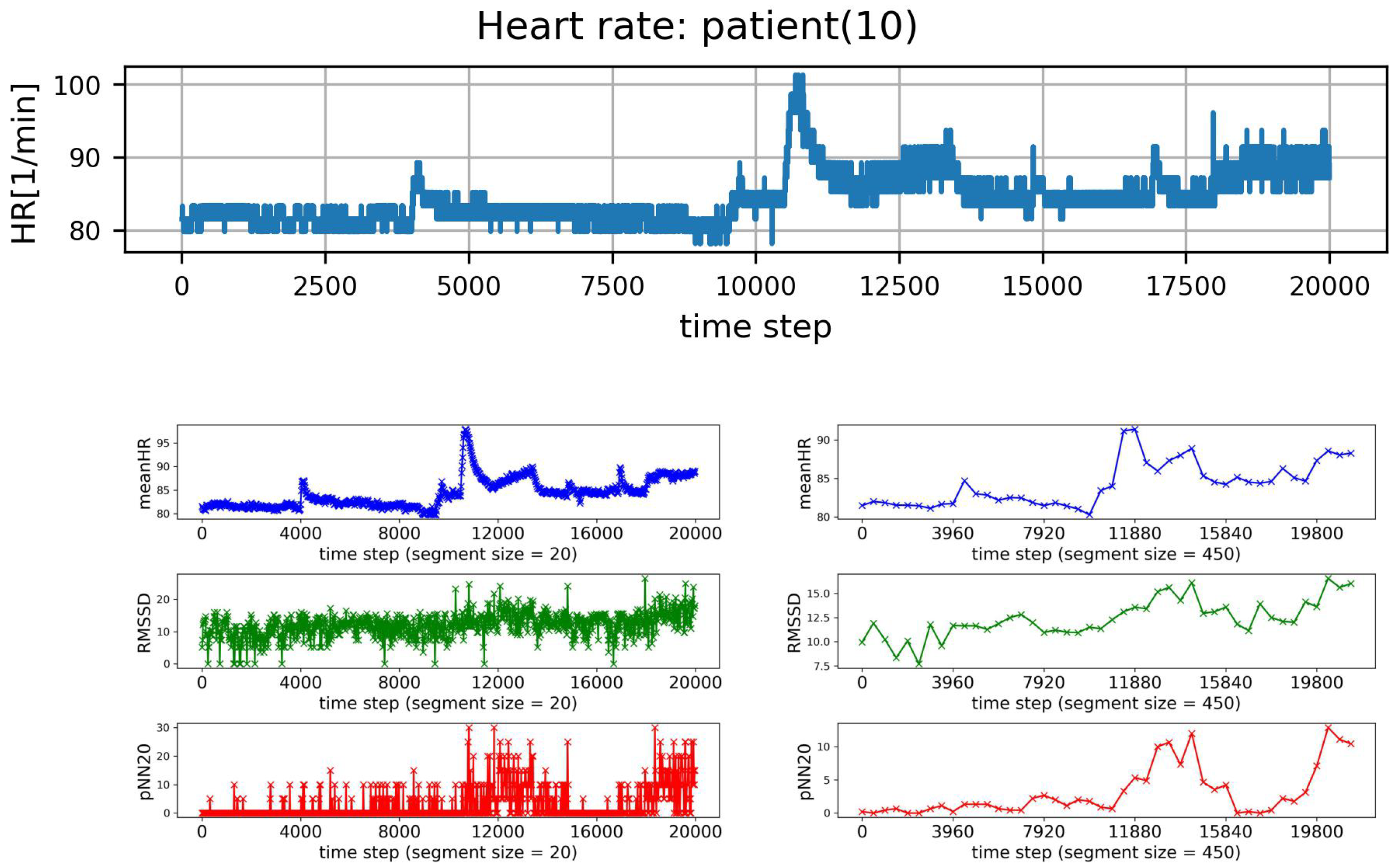
Figure 1. Plots of subsequent 20,000 HR points of a typical signal recorded from HTX patient (top row), and resulting values of meanHR, RMSSD, and pNN20 obtained in consecutive segments of RR intervals. The segment size is: (left column) s = 20 , (right column) s = 450 RR intervals.
Biomedinformatics 03 00015 g001
Figure 2. The contour plots of probability (in logarithmic scale) to meet an event: Δ i followed by Δ j , obtained from signals of RR intervals pooled in groups of healthy persons and HTX patients. Δ means the magnitude in ms of a deceleration, Δ > 0 , or acceleration, Δ < 0 .
Biomedinformatics 03 00015 g002
Figure 3. The contour plots of the Shannon entropy matrix E for probability distribution to meet an event: Δ i followed by Δ j . Results were obtained from signals of RR intervals pooled in groups of healthy persons and HTX patients. Δ means the magnitude in ms of a deceleration, Δ > 0 , or acceleration, Δ < 0 .
Biomedinformatics 03 00015 g003
Figure 4. The contour plots of probability of the transition Δ i Δ j  while being in Δ i , obtained from signals of RR intervals pooled in groups of healthy persons and HTX patients. Δ means the magnitude in ms of a deceleration, Δ > 0 , or acceleration, Δ < 0 .
Biomedinformatics 03 00015 g004
Figure 5. The contour plots of the entropy of transition rates matrix S _ T quantifying Markovian dynamics for an event: Δ i followed by Δ j . obtained from signals of RR intervals pooled in groups of healthy persons and HTX patients. Δ means the magnitude in ms of a deceleration, Δ > 0 , or acceleration, Δ < 0 .
Biomedinformatics 03 00015 g005
Figure 6. The contour plots of matrix sTE quantifying the memory effects in probability to observe a sequence of events: Δ i followed by Δ j . Results were obtained from signals of RR intervals pooled in groups of healthy persons and HTX patients. Δ means the magnitude in ms of a deceleration, Δ > 0 , or acceleration, Δ < 0 .
Biomedinformatics 03 00015 g006
Figure 7. Kruskal–Wallis test results for HRV measures estimated from windows with the highest SDNN (left) and dependence of the group medians for e(dad), p(da), e(da), pNN20, and RMSSD, consecutively, on segment size (right). Left: names of HRV measures against the segment size, red asterisk indicates segment size for which a statistically significant difference was found, green asterisk indicates a result supported by more than 70% in the bootstrap test. Only measures that discerned groups at least once are listed. Right: The five most statistically confirmed measures of HRV differentiating the studied groups are shown. A black cross indicates the size of a window for which a statistically significant difference was found. A green cross indicates a result supported by the bootstrap test (70%).
Biomedinformatics 03 00015 g007
Figure 8. Kruskal–Wallis test results for HRV measures estimated from windows with the smallest SDNN (left) and dependence of the group medians for p(da), LF and VLF, consecutively, on segment size (right). Plots present the group medians which differentiated the studied groups in at least five segments. See the caption in Figure 7 for other details of the used notation.
Biomedinformatics 03 00015 g008
Figure 9. Kruskal–Wallis test results for HRV measures estimated from windows with the highest HR (left) and dependence of the group medians for e(ad), e(da), e(dad), ShE_1 and sTE, consecutively, on segment size (right). The five most statistically confirmed measures of HRV differentiating the studied groups are shown. See the caption in Figure 7 for other details of the used notation.
Biomedinformatics 03 00015 g009
Figure 10. Kruskal–Wallis test results for HRV measures estimated from windows with the smallest HR (left) and dependence of the group medians for VLF, p(a), and p(zero), consecutively, on segment size (right). Only the measures that differentiated the studied groups in at least five segments are presented. See the caption in Figure 7 for details of the used notation.
Biomedinformatics 03 00015 g010
Figure 11. Kruskal–Wallis test results for std of the whole HRV series (left) and dependence of the group medians of the std of series p(a), p(ad), PIP, p(a), p(zero) and e(da), consecutively, on segment size (right). Only the measures that differentiated the studied groups in at least five segments are presented. See the caption in Figure 7 for details of the used notation.
Biomedinformatics 03 00015 g011
Figure 12. Kruskal–Wallis test results for SampEn of the whole HRV series (left) and dependence of the group medians of the SampEn of series for VLF, p(a), and p(zero), consecutively, on segment size (right). The five most statistically confirmed measures of HRV differentiating the studied groups are shown. See the caption in Figure 7 for details of the used notation.
Biomedinformatics 03 00015 g012
Table 1. Demographic and echo characteristics of patients. Data are expressed as the mean ± std error or as the number (percentage).
CharacteristicNGCRHDifference between Groups
number of patients12 (29%)22 (52%)8 (19%)
age at transplantation,43 ± 1449 ± 1148 ± 11NS
male gender, n10 (83%)20 (91%)8 (88%)
BMI26± 426 ± 627 ± 5NS
BSA1.9 ± 0.12.0 ± 0.22.0 ± 0.2NS
LVMI (g/m 2 )82 ± 1092 ± 14122 ± 9(NG,H) (CR,H)
LVM (g)156 ± 25184 ± 28245 ± 33all pairs are different
RWT0.39 ± 0.030.53 ± 0.070.50 ± 0.07(NG,H) (NG,CR)
EF %64 ± 364 ± 467 ± 10NS
LV SV (mL)66 ± 760 ± 1176 ± 16NS
Abbreviations used: NG, normal geometry; CR, concentric remodeling; H, hypertrophy; BMI, body mass index, BSA, body surface area; LVMI, left ventricular mass index; LVM, left ventricular mass; RWT, relative wall thickness; EF, ejection fraction; LV SV, left ventricle stroke volume; NS, group difference is statistically insignificant in Kruskal–Wallis test.
Table 2. List of estimated HRV measures.
standard measures:long–term time domainmeanRR, meanHR,
based on a series of SDNN, stdHR
{ R R ( t ) }
frequencyPS, VLF, LF, HF
short-term time domainRMSSD, pNN50, pNN20
increment pattern measures:probability of patternsp(zero), p(a), p(d),
based on series of increments p(aa), p(ad), p(da), p(dd),
between consecutive RR intervals: p(aaa), p(ada), p(dad), p(ddd)
{ Δ R R ( t ) }
a is an acceleration if Δ R R ( t ) 8 msfragmentation measuresPIP = p(ad)+p(da)
d is a deceleration if Δ R R ( t ) 8 ms. PAS = p(ada) + p(dad)
Otherwise an increment is zero PSS = 1 – [p(aaa) +p(ddd)]
entropic measures:
–Shannon entropy of L-length patternsShE_L for L=1,2,3
–dynamics by entropy patterns,S_T = ShE_1 - ShE_2,
sTE = ShE_2 - ShE_3 – S_T
–partial entropy of patternse(aa), e(ad), e(da), e(dd),
e(aaa), e(ada), e(dad), e(ddd)
Table 3. Medians and their first and third quartiles estimated for the groups of healthy individuals, and NG, CR, H for HRV measures listed in Table 2, together with the p-value from the Kruskal–Wallis test for differences between HTX groups. In brackets() the bootstrap support value is provided if observed.
HRVHealthyHTX GroupsKruskal–Wallis
IndexCovealsNGCRHTest p for HTX
meanRR958 [870, 1067]697 [679, 819]688 [635, 791]714 [683, 757]p = 0.587
meanHR62.85 [56.95, 69.80]86.23 [73.35, 88.39]87.62 [75.88, 94.72]84.16 [79.36, 88.04]p = 0.542
SDNN87.10 [72.18, 102.30]22.17 [20.10, 31.66]28.44 [20.77, 35.89]31.15 [25.65, 35.17]p = 0.415
stdHR6.577 [5.849, 7.253]2.853 [1.953, 3.330]3.807 [2.322, 4.162]3.266 [3.193, 4.185]p = 0.128
PS3.384 [3.033, 3.755]2.432 [2.114, 2.916]2.558 [2.373, 2.671]2.569 [2.358, 2.750]p = 0.938
VLF1.392 [1.308, 1.507]1.112 [0.929, 1.167]1.180 [1.054, 1.323]1.110 [1.066, 1.200]p = 0.338
LF1.000 [0.862, 1.281]0.265 [0.224, 0.366]0.297 [0.244, 0.369]0.302 [0.257, 0.399]p = 0.603
HF0.868 [0.668, 1.051]1.005 [0.708, 1.235]0.958 [0.786, 1.192]1.035 [0.855, 1.326]p = 0.859
RMSSD32.12 [22.85, 46.87]9.879 [7.308, 11.29]7.189 [6.593, 9.669]9.575 [7.012, 12.24]p = 0.328
pNN506.215 [2.435, 18.76]0.025 [0.004, 0.059]0.015 [0.005, 0.025]0.040 [0.020, 0.185]p = 0.099 (0.05)
pNN2039.68 [29.89, 55.69]3.815 [2.001, 5.566]0.583 [0.184, 3.109]3.908 [0.320, 4.885]p = 0.244
p(zero)0.145 [0.101, 0.181]0.358 [0.317, 0.456]0.448 [0.405, 0.469]0.430 [0.352, 0.489]p = 0.289
p(a)0.441 [0.415, 0.465]0.325 [0.274, 0.353]0.273 [0.265, 0.296]0.294 [0.257, 0.318]p = 0.174
p(d)0.423 [0.398, 0.446]0.307 [0.272, 0.340]0.276 [0.264, 0.301]0.276 [0.257, 0.323]p = 0.415
PSS0.883 [0.853, 0.919]1.000 [0.996, 1.000]1.000 [0.998, 1.000]0.999 [0.997, 1.000]p = 0.862
p(aa)0.183 [0.165, 0.207]0.028 [0.007, 0.049]0.017 [0.009, 0.029]0.021 [0.009, 0.038]p = 0.915
e(aa)1.019 [0.859, 1.175]0.137 [0.038, 0.232]0.077 [0.045, 0.118]0.097 [0.043, 0.169]p = 0.857
p(aaa)0.058 [0.039, 0.078]0.000 [0.000, 0.003]0.000 [0.000, 0.001]0.001 [0.000, 0.001]p = 0.625
e(aaa)0.461 [0.312, 0.621]0.003 [0.001, 0.020]0.002 [0.000, 0.008]0.005 [0.000, 0.008]p = 0.672
p(dd)0.176 [0.152, 0.195]0.021 [0.005, 0.038]0.016 [0.009, 0.028]0.012 [0.008, 0.035]p = 0.992
e(dd)1.006 [0.871, 1.127]0.109 [0.027, 0.187]0.069 [0.046, 0.118]0.064 [0.039, 0.157]p = 0.999
p(ddd)0.058 [0.039, 0.069]0.000 [0.000, 0.001]0.000 [0.000, 0.001]0.000 [0.000, 0.002]p = 0.996
e(ddd)0.477 [0.302, 0.574]0.002 [0.000, 0.007]0.001 [0.000, 0.007]0.001 [0.000, 0.013]p = 0.993
PAS0.125 [0.082, 0.189]0.165 [0.132, 0.207]0.156 [0.136, 0.165]0.161 [0.146, 0.170]p = 0.704
PIP0.373 [0.321, 0.448]0.341 [0.328, 0.385]0.325 [0.313, 0.333]0.330 [0.314, 0.369]p = 0.084 (0.07)
p(ad)0.188 [0.170, 0.229]0.168 [0.154, 0.198]0.159 [0.152, 0.169]0.165 [0.160, 0.173]p = 0.418
e(ad)1.025 [0.848, 1.309]0.557 [0.448, 0.709]0.427 [0.387, 0.493]0.516 [0.392, 0.611]p = 0.209
p(da)0.185 [0.154, 0.212]0.175 [0.171, 0.203]0.162 [0.158, 0.175]0.164 [0.157, 0.185]p = 0.045 (0.72)
e(da)0.938 [0.834, 1.281]0.594 [0.462, 0.706]0.433 [0.399, 0.593]0.528 [0.391, 0.621]p = 0.225
p(ada)0.055 [0.040, 0.092]0.086 [0.073, 0.105]0.080 [0.068, 0.083]0.079 [0.074, 0.087]p = 0.618
e(ada)0.441 [0.338, 0.682]0.355 [0.308, 0.549]0.279 [0.252, 0.323]0.293 [0.257, 0.409]p = 0.131 (0.04)
p(dad)0.070 [0.035, 0.100]0.077 [0.066, 0.104]0.077 [0.069, 0.082]0.080 [0.072, 0.086]p = 0.755
e(dad)0.534 [0.282, 0.785]0.325 [0.280, 0.513]0.273 [0.249, 0.326]0.307 [0.267, 0.393]p = 0.229
ShE_37.321 [6.915, 8.250]4.049 [3.137, 4.546]3.388 [3.079, 4.036]3.546 [3.016, 4.361]p = 0.52
ShE_25.146 [4.792, 5.849]2.945 [2.267, 3.123]2.374 [2.169, 2.869]2.542 [2.147, 3.073]p = 0.437
ShE_12.663 [2.421, 3.019]1.613 [1.280, 1.637]1.279 [1.190, 1.525]1.404 [1.179, 1.629]p = 0.27
S_T2.507 [2.352, 2.844]1.339 [0.970, 1.511]1.099 [0.988, 1.307]1.138 [0.970, 1.438]p = 0.716
sTE0.302 [0.204, 0.487]0.138 [0.093, 0.205]0.097 [0.082, 0.120]0.131 [0.108, 0.160]p = 0.106 (0.02)
Disclaimer/Publisher’s Note: The statements, opinions and data contained in all publications are solely those of the individual author(s) and contributor(s) and not of MDPI and/or the editor(s). MDPI and/or the editor(s) disclaim responsibility for any injury to people or property resulting from any ideas, methods, instructions or products referred to in the content.