Article

Adjusted Sample Size Calculation for RNA-seq Data in the Presence of Confounding Covariates

1
Department of Anatomical Sciences and Neurobiology, University of Louisville, Louisville, KY 40202, USA
2
Kentucky IDeA Network for Biomedical Research Excellence Bioinformatics Core, University of Louisville, Louisville, KY 40202, USA
3
Department of Bioinformatics and Biostatistics, University of Louisville, Louisville, KY 40202, USA
4
Department of Computer Science and Engineering, University of Louisville, Louisville, KY 40202, USA
5
Department of Medicine, University of Louisville, Louisville, KY 40202, USA
*
Author to whom correspondence should be addressed.
BioMedInformatics 2021, 1(2), 47-63; https://doi.org/10.3390/biomedinformatics1020004
Submission received: 23 March 2021 / Revised: 18 June 2021 / Accepted: 21 June 2021 / Published: 29 June 2021

Abstract

:
Sample size calculation for adequate power analysis is critical in optimizing RNA-seq experimental design. However, the complexity increases for directly estimating sample size when taking into consideration confounding covariates. Although a number of approaches for sample size calculation have been proposed for RNA-seq data, most ignore any potential heterogeneity. In this study, we implemented a simulation-based and confounder-adjusted method to provide sample size recommendations for RNA-seq differential expression analysis. The data was generated using Monte Carlo simulation, given an underlined distribution of confounding covariates and parameters for a negative binomial distribution. The relationship between the sample size with the power and parameters, such as dispersion, fold change and mean read counts, can be visualized. We demonstrate that the adjusted sample size for a desired power and type one error rate of α is usually larger when taking confounding covariates into account. More importantly, our simulation study reveals that sample size may be underestimated by existing methods if a confounding covariate exists in RNA-seq data. Consequently, this underestimate could affect the detection power for the differential expression analysis. Therefore, we introduce confounding covariates for sample size estimation for heterogeneous RNA-seq data.

1. Introduction

Sample size and power are important factors for planning a biological experiment using high-throughput sequencing technologies for differential gene expression (RNA-seq). Larger sample sizes typically provide a more accurate estimate of the differential gene expression with high confidence. However, since RNA-seq techniques are costly, a large sample size is sometimes not feasible when limited research budgets are considered. Therefore, an optimized sample size is desired to achieve a specific power for detecting gene expression changes within realistic budget constraints. Moreover, since read depths often vary significantly between runs, this particular technical variation also needs to be taken into consideration in any sample size estimation.
With the rapid growth of RNA-seq studies, a number of sample size estimation methods and software tools have been proposed [1,2,3,4,5,6,7,8,9]. However, these methods have their limitations and assumptions. Since RNA-seq data are short read counts, Fang and Cui (2011) used a Poisson distribution to derive a sample size calculation formula combined with a Wald-like Z-statistic test on a single gene [1]. Li et al. (2013) extended sample size calculation methods using a Wald test, a score test and a likelihood ratio test (LRT) based on testing a single gene or multiple genes [2]. However, the studies [10,11] found that a Poisson distribution may not be appropriate to model gene read counts in RNA-seq data due to over-dispersion as a result of natural biological variation. To address this issue, a negative binomial (NB) distribution combined with an exact test and/or likelihood ratio test (LRT) was proposed to model RNA-seq data in differential gene expression analysis [10,11,12]. Subsequently, other sample size calculation methods were proposed using an NB distribution [3,4,5,7,8]. Hart et al. (2013) proposed a sample size calculation method using a score test based on a single gene [7] and Liu et al. (2014) further proposed sample size calculations using an exact test implemented in edgeR [8]. Later, Li et al. (2013) developed the RnaSeqSampleSize R package based on TCGA data [13]. Similarly, Ching et al. [6] and Wu et al. [14] performed a power analysis implemented in DESeq2 and/or edgeR while controlling false discovery rate (FDR). These methods employed the common analysis approaches with the aid of DESeq2 or edgeR. However, these studies have reported the actual FDR resulting from NB-based methods such as DESeq2 and edgeR was inflated in many cases [15,16,17,18,19,20]. To address this issue, Yu et al. [9] proposed a power analysis based mainly on simulation studies for a given desired type I error rate. In addition, several sample size calculations were developed using a Wald test, a log-transformed Wald test and an analytical method using a log LRT test based on a single gene or multiple genes with controlling FDR [4]. Recently, we proposed a method for sample size calculation using a generalized linear model (GLM) with an NB distribution where the dispersion was estimated on the basis of a variance–covariance matrix between two groups [5]. However, the sample sizes estimated in all these studies may only be appropriate for homogeneous data with tightly controlled conditions.
With a GLM, it is very important to identify independent covariates and confounding covariates in an experimental design. The difference in covariates is that the independent covariates can be controlled by experimental design, while the confounding covariates cannot be controlled. These confounding covariates from heterogeneous data commonly exist in clinical RNA-seq studies such as cancer and other disease-associated datasets. For example, age and sex are common confounding factors in RNA-seq, as are more complex variables such as diet, exercise, and environmental influences. Existing methods for determining sample size are suitable for cell lines or animal studies where other variables can be tightly controlled. However, when a confounding covariate exists in an experiment, such as with nearly all human studies, these methods may underestimate the sample size, eventually affecting the statistical power of the experiment.
To address this issue, we introduce confounder-adjusted sample size calculation using a simulation-based empirical approach. These simulated data are based on a NB regression model with the aid of the rnbinom and glm.nb functions of the MASS R package. The confounding covariate of the simulated study is defined as a continuous variable (i.e., age) or a categorical variable (i.e., sex). We illustrate how to calculate age and sex-adjusted sample size and power using the public colon adenocarcinoma (COAD) data downloaded from Broad GDAC Firehouse. The method described here can provide an additional option for clinical researchers to determine sample size in designing complex RNA-seq experiments.

2. Materials and Methods

2.1. A Generalized Linear Model with a NB Distribution

A Generalized liner model (GLM) has been widely applied in scientific fields [21]. For a single gene in RNA-seq data, the independent random sample ( Y i j ) for the sample j  j = 1 ,   , n i   in condition i ( i = 0 ,   1 ) is assumed to have an identical NB distribution, such as Y i j ~ N B µ i j , ϕ . Thus, the probability mass function of the observation y i j is defined as:
P ( y i j ) = Γ ϕ 1 + y i j Γ ϕ 1 y i j ! ϕ µ i j 1 + ϕ µ i j y i j 1 1 + ϕ µ i j ϕ 1 ,
where   µ i j = s i j γ i ,   s i j is the size factor for normalizing read depth, γ i is the true expression of the gene and is unknown, and µ i j is the expected mean expression.
For the purpose of power and sample size calculation within the framework of a GLM, we defined the expected mean read counts ( µ i j ) for y i j by a log link function as:
log   u i j = log   s i j + ψ 0 + ψ 1 Z i   + b L i + λ X i ,
where the covariate Z i , a treatment group indicator, takes value Z 0   = 0 if i = 0   for the control group and Z 1   = 1 if i = 1 for the treatment group. The multiple covariates L i   and X i , confounding variables, are assumed to be a continuous variable and/or categorical variable, respectively, and the quantity log   s i j denotes an offset. The true expression of γ i is analyzed directly by the GLM and can also be expressed as:
log   γ i = ψ 0 + ψ 1 Z i   + b L i + λ X i   ,
Thus, the true expression γ 0 and γ 1 from Equation (3) can be obtained as:
γ 0 = e ψ 0 + b L 0 + λ X 0   ,   γ 1 = e ψ 0 + ψ 1 + b L 1 + λ X 1     and   γ 1 γ 0 = e ψ 1 + b L 1 L 0 + λ X 1 X 0
Replacing u i j = s i j e ψ 0 + ψ 1 + b L i + λ X i   = s i j γ i in Equation (1), the log-likelihood function is expressed as:
l = i = 0 1 j = 1 n i log   Γ ϕ 1 + y i j Γ ϕ 1 y i j ! + y i j log   ϕ s i j e ψ 0 + ψ 1 Z i + b L i   + λ X i   y i j + 1 ϕ log 1 + ϕ s i j e ψ 0 + ψ 1 Z i + b L i   + λ X i  
The covariant-adjusted coefficient ψ 1 is expected to be different for the log count of the gene between the treatment and the control groups. In this study, the p-value along with the coefficient ψ 1 obtained from the glm.nb function is used to determine if the gene read counts in the treatment group is statistically significant from the control.

2.2. Simulation-Based Studies

The RNA-seq data relies on parameters to be simulated. The sample size and actual power are determined by the DEG analysis for the different parameter settings. In this study, we considered the presence of both single and dual confounding variables.

2.2.1. Sample Size Estimation for a Single Gene

Simulation of single confounding factor data: For a single confounding variable, we have two sets of linear predictors in the form log   γ 0 = ψ 0 + λ X 0   and   log   γ 1 = ψ 0 + ψ 1 + λ X 1   for the control and treatment group, respectively. For dual confounding variables, they are log   γ 0 = ψ 0 + b L 0 + λ X 0   and   log   γ 1 = ψ 0 + ψ 1 + b L 1 + λ X 1   . Three scenarios in single confounding variables are described as follows. In the first scenario, we consider the confounding covariate X 0 , given Z 0 = 0 , and X 1 ,   given Z 1 = 1 ,   follows a normal distribution with equal and/or unequal means and variance resulting in four settings: N 0 (0, 1) and N 1 (0,   1.5 2 ), N 0 (0, 1) and N 1 (1.5,1),   N 0 (40, 5 2 ) and N 1 (42,   5 2 ), N 0 (40, 2 2 ) and N 1 (42,   5 2 ) and N 0 (30, 3 2 ) and N 1 (40, 3 2 ) for the control and treatment group, respectively. In the second scenario, we consider the covariate X 0 and X 1   follows a Poisson distribution with equal and/or unequal means resulting in three settings: P o i s 0 (10) and P o i s 1 (12), P o i s 0 (10) and P o i s 1 (15) and P o i s 0 (25) and P o i s 1 (20). Two settings are a mixture of normal and Poisson distributions: P o i s 0 (10) and N 1 (12, 1) and P o i s 0 (10) and N 1 (12, 10) for the control and treatment groups, respectively. This is assumed in a rare situation. In the last scenario, we consider the confounding covariate X 0 and X 1   as categorical variables, each taking the binary value 0 or 1. There are six different settings, including I(0.25, 0.25, 0.25, 0.25), II(0.2, 0.3, 0.3, 0.2), III(0.3, 0.2, 0.2, 0.3), IV(0.1, 0.4, 0.4, 0.1) and V(0.4, 0.1, 0.1, 0.4) and VI(0.1, 0.3, 0.4, 0.2). Each of the six settings corresponds to the different proportion of the single covariate in two groups (0,1) such as sex (male, female). Three of them were originally proposed by Self Steven for a GLM with a Bernoulli distribution [22]. I(0.25, 0.25, 0.25, 0.25) is assumed from a homogeneous confounding covariate, and VI(0.1, 0.3, 0.4, 0.2) is assumed completely unequal proportion in control and treatment groups
Simulation of dual confounding variables: For the dual confounding variables, one confounding covariate ( L 0 and L 1 ) is set to follow a normal distribution with equal and/or unequal mean and variance resulting in two settings: N 0 (0, 1) and N 1 (1.5, 1), and   N 0 (40, 2 2 ) and N 1 (42,   5 2 ). The second confounding covariate ( X 0 and X 1 ) is set as a categorical variable with four different settings: I(0.2, 0.3, 0.3, 0.2), II (0.1, 0.4, 0.4, 0.1), III (0.1, 0.3, 0.4, 0.2) and V(0.15, 0.35, 0.35, 0.15).
Parameter estimation: In the simulation, the alternative hypothesis test on a single gene is that the gene is considered differentially expressed when ψ 1 0 . In this study, the fold change (ρ) is set to be 0.5 ,     1.5 ,     2.0   or   3.0 , corresponding to ψ 1 0 . The minimum mean read count of the DEGs in the control group, µ 0 , is set to be 5 and 10. The ratio of mean size factors, w = s ¯ 1 s ¯ 0 , is set to be 1 for normalized RNA-seq data and w 1 for unnormalized RNA-seq data; the constant dispersion parameter ϕ   is set to be 0.1 ,     0.2   or   0.5 ; the ratio of sample sizes is set to be k = 1 for a balanced design.
Simulation of RNA-seq data: For a fixed sample size of n given the designed parameter setting, two groups of NB random samples are generated. For the control group, the random samples are generated given the parameters n 0 ,   µ 0 and ϕ . For the treatment group, the random samples are generated given the parameters n 1 = k n 0 , µ 1 = ρ w ,   µ 0 and ϕ . k 1 indicates an imbalanced design. Given a fixed n and a specified covariate distribution for the control and treatment groups, the two datasets are randomly and independently generated.
Sample size and power estimation: For a given model and covariate distribution, sample sizes are estimated by testing the hypothesis: H 0 :   ψ 1 = 0 vs. H 1 :   ψ 1 0 with significance level α and power 0.80. Each Monte Carlo estimate of power associated with a fixed sample size is imputed under different scenarios and settings through 1000 independently generated datasets.
The procedure for sample size and power estimation can be briefly summarized as the following steps:
  • Obtain the pre-specified parameters, such as fold change (ρ), the ratio of size factors w and the ratio of sample sizes k between two-sample groups.
  • Specify a desired statistical power (i.e., 0.80) and significance level α 0.05.
  • Simulate control and treatment groups RNA-seq data given the mean counts in the control group ( u 0 ) and common dispersion (ϕ) for a fixed n using an NB distribution with the aid of the rnbinom function in R.
  • Simulate a confounding covariate under different scenarios given a fixed n and distribution with the aid of the rnorm function for a normal distribution, the rpois function for a Poisson distribution and rnbinom for a binomial distribution for a categorical confounder.
  • Fit the GLM with a NB distribution using the R glm.nb function.
  • Obtain the coefficient ψ 1 along with the standard error, z-score and p-value for statistical test on ψ 1 from the simulated data set. For a two-sided test, record whether a p-value   α / 2 in testing a single gene or p-value   α * / 2   in testing multiple genes.
  • Repeat steps 3–6 for 1000 times and impute the statistical power for the fixed sample size.
  • Repeat steps 3–7 by increment of sample size by one ( n = n + 1 ) if the power is smaller than 0.7999 0.80 . Stop when a desired statistical power is obtained and then record the sample size n and the actual power.
The R source codes are provided for the illustration of estimating the empirical power and sample size n (Supplementary File S2).

2.2.2. Sample Size Estimation for Controlling FDR in Testing Multiple Genes

In this study, the size α for a single gene has been adjusted for testingmultiple genes, which has been implemented in recent studies [3,5]. A similar approach to the previous studies was used to calculate the new size α by incorporating FDR [2,3,4]. Briefly, given a nominal FDR at a specified level f of 0.05, the adjusted significance level α * for the expected number of true rejection t 1   is defined
α * = t 1 f t 0 1 f   ,
where t 0 is the number of true null hypotheses. Replacing the size α 0.05 in testing a single gene with a smaller α * in simulation study from steps 1 to 8, the expected sample sizes and estimates of power corrected by FDR at level f are then obtained.

3. Results

The sample size n (biological replicates) and actual power are calculated given a significance level alpha of 0.05 and a desired 80% power for a single gene or multiple genes at a controlling FDR of 0.05. Monte Carlo estimates are based on empirical data generated for different parameter settings. We performed a GLM with an NB distribution incorporating potential confounding covariates denoted either as a categorical or continuous variable at a normal and Poisson distribution. The Wald-like z test in glm.nb with a log link function is used for testing the significance of the coefficient ψ 1 with the inverse of dispersion 1/ϕ. ψ 1 is the coefficient of the treatment group as an independent variable in a GLM. ϕ is the dispersion parameter in an NB distribution. The variance of NB distribution is a function of its mean and additional overdispersion of ϕ. The genes between the two groups are considered significantly different when the p-value is ≤ α/2 for a two-sided test. The procedures are repeated 1000 times, and the power is calculated as the percentage of the number of times that the null hypothesis H0 is rejected. Table 1 summarizes the results under different scenarios with a variety of parameter settings, as illustrated in Figure 1, Figure 2, Figure 3, Figure 4, Figure 5, Figure 6, Figure 7 and Figure 8.

3.1. Sample size n and actual power from a single confounder variable for testing single gene

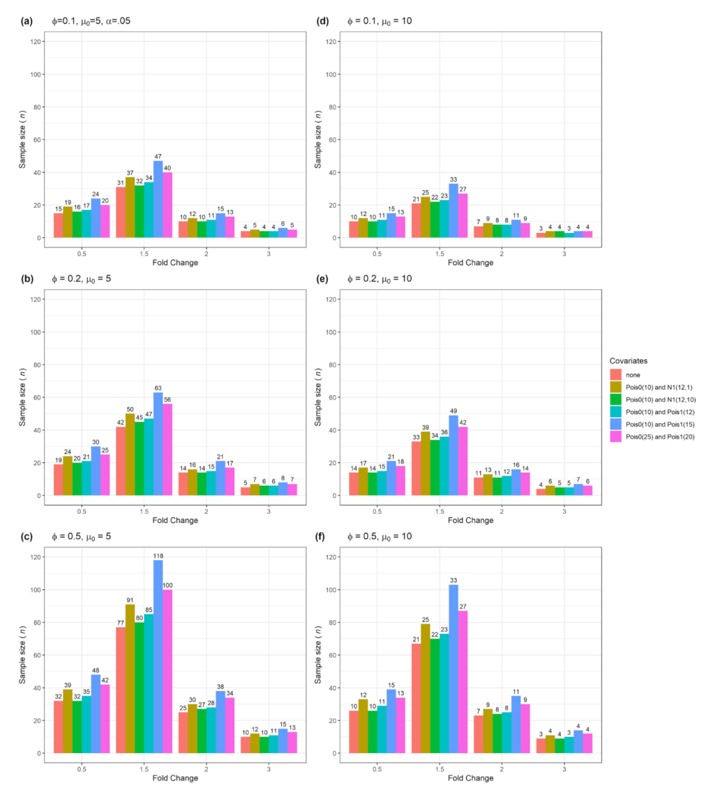
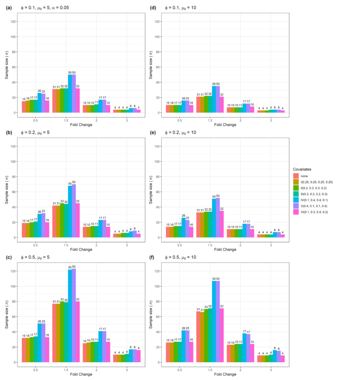
The bar graphs in Figure 1, Figure 2 and Figure 3 illustrate the sample size n versus the fold change ρ with fixed ϕ and µ 0   adjusted by different covariates for testing a single gene. The actual power calculated from the simulation is ≥ 0.8. The color-coded bars in Figure 1 represent confounding covariates in a normal distribution with equal/unequal mean and variance between two groups. The height of the bars illustrated in the figures represents the number of the sample size. We first observe that the n decreases as the fold change ρ increases from 1.5 to 3, where the ρ of 0.5 indicates a 2-fold down-regulated gene. The figures show that a much larger n is required for the gene that has a fold change of 1.5 compared to a fold change of 2 or 3, which is expected. Given a fixed µ 0 and ρ, n increases as ϕ increases from 0.1 to 0.5 (Figure 1a–f). This is also expected, which indicates that a larger n is required for a higher variation of samples. We also observed that n decreases as the read count µ 0 increases from 5 to 10 (Figure 1a–f), given a fixed ρ and ϕ or vice versa. Since µ 0 represents the abundance of gene expression, this suggests that a larger n for a lowly expressed gene is required in order to achieve an empirical power close to 0.80 in the DEG analysis. Furthermore, we need to point out that the values of n are not similar for a fold change of 0.5 and 2 because there is no symmetry between laws in H 0 and H 1 .   Given different confounding covariates, similar changes of n for the parameter settings (ρ,   µ 0 and ϕ) are observed in Figure 2 and Figure 3.
Next, we examined the change of n between the confounding covariates in Figure 1. We observed that the confounder-adjusted n is generally larger than that for a non-adjusted one. The colored-coded bars show that the adjusted n obtained from the confounding covariate with the difference of the mean in two groups, such as N 0 (0, 1) and N 1 (1.5, 1) in green, N 0 (40, 5 2 ) and N 1 (42,   5 2 ) in cyan and N 0 (30, 3 2 ) and N 1 (40,   3 2 ) in magenta, are much larger than a non-adjustment in orange. However, the n obtained from the equal mean confounders N 0 (0, 1) and N 1 (0,   1.5 2 ) in yellow, and N 0 (40, 2 2 ) and N 1 (40,   5 2 ) in azure either has no effect or a small effect compared to the non-adjustment. The confounding covariates corresponding to the adjusted n from largest to smallest are: N 0 (30, 3 2 ) and N 1 (40,   3 2 ) > N 0 (0, 1) and N 1 (1.5, 1) > N 0 (40, 5 2 ) and N 1 (42,   5 2 )   N 0 (0, 1) and N 1 (0,   1.5 2 ), and N 0 (40, 2 2 ) and N 1 (40,   5 2 ). This indicates that a larger n is required in highly heterogeneous data to achieve a desired power compared to homogeneous data (no-confounder present), which is expected.
Figure 2 displays the n obtained when the confounding covariate follows a Poisson or normal distribution with different settings between two groups. The color-coded bars illustrate that a larger n is required for all of the confounding covariates relative to when there was no confounder present. The n changes with the characteristics of confounding covariate heterogeneity (Figure 1 and Figure 2) are similar. We observed that the greater the mean difference of the confounders between the two groups, the larger n is required to achieve a desired power. The confounding covariates corresponding to the adjusted n from largest to smallest are: P o i s 0 (10) and P o i s 1 (15) in azure > P o i s 0 (25) and P o i s 1 (20) in magenta >   P o i s 0 (10) and N 1 (12,1) in yellow >   P o i s 0 (10) and P o i s 1 (12) in cyan >   P o i s 0 (10) and N 1 (12,   10 2 ) in green. It is interesting to observe that a different distribution of confounders between the two groups, such as a Poisson distribution P o i s 0 (10) with a mean and variance of 10 and normal distribution N 1 (12,1) with a mean of 12 and variance of 1, requires a larger n compared with the same distribution of the covariate ( P o i s 0 (10) and P o i s 1 (12)) or different distribution of the covariate with same variance P o i s 0 (10) and N 1 (12,   10 2 ). This suggests that high variances in confounding covariates can affect sample size.
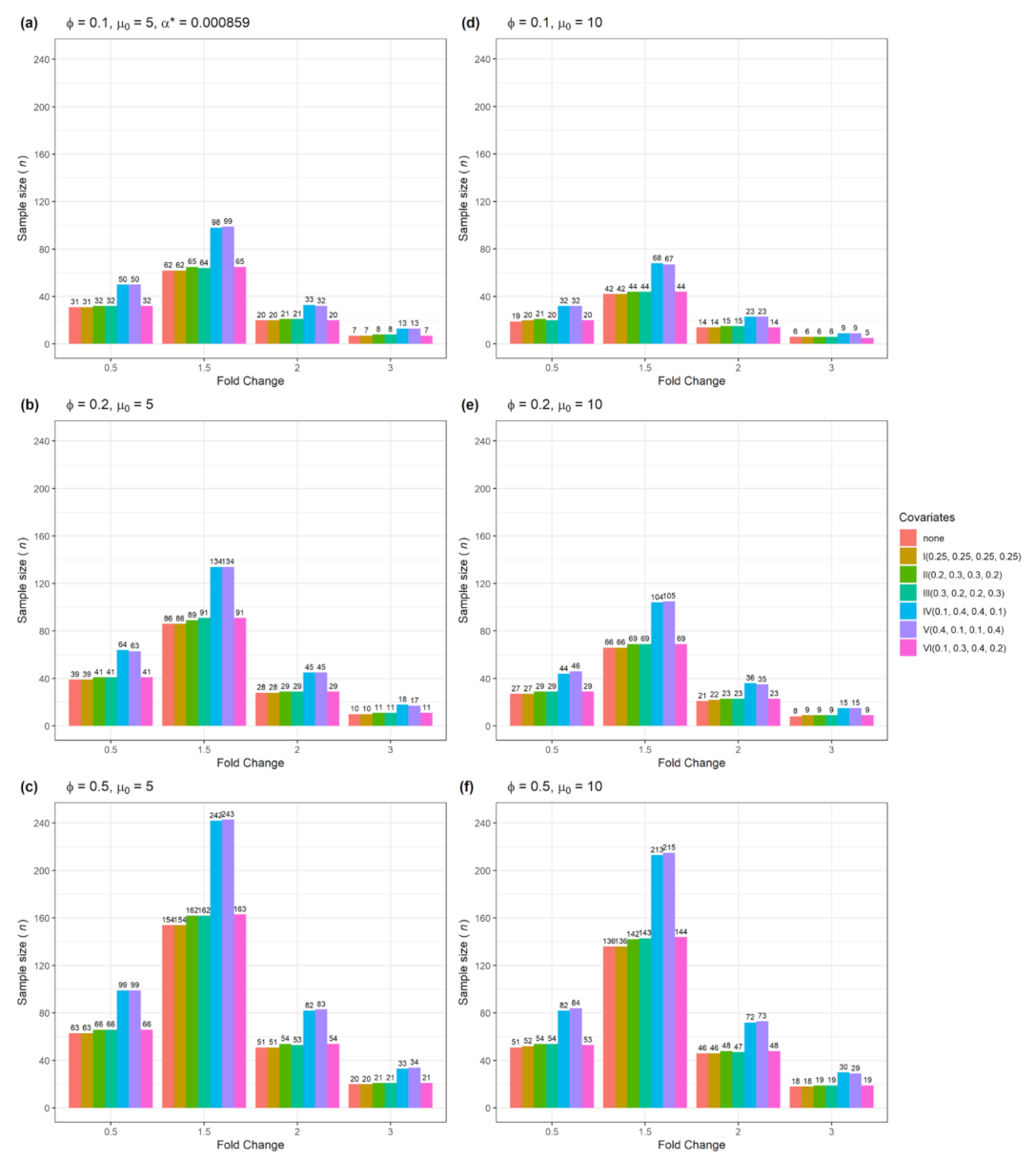
Figure 3 lists the n calculated from the simulated data when the covariate is a categorical confounder. In this scenario, the confounder covariate X 0 and X 1   take the binary value 0 and 1 for the control and treatment group, respectively. Six different settings are denoted as I(0.25, 0.25, 0.25, 0.25), II(0.2, 0.3, 0.3, 0.2), III(0.3, 0.2, 0.2, 0.3), IV(0.1, 0.4, 0.4, 0.1), V(0.4, 0.1, 0.1, 0.4) and VI(0.1, 0.3, 0.4, 0.2). Each of the six settings corresponds to the different proportion of the single confounder in two groups (0,1) such as sex (male, female). For example, the IV(0.1, 0.4, 0.4, 0.1) has high disproportion between control and treatment groups, which stands for 10% female and 40% male in the control group, and 40% female and 10% male in the treatment group. Compared with no confounders or an equal proportion between the two groups (I (0.25, 0.25, 0.25, 0.25)), we observed a larger n at high proportion between the two groups is required. The categorical confounding covariates corresponding to the adjusted n from largest to smallest are: IV(0.1, 0.4, 0.4, 0.1) in cyan and V(0.4, 0.1, 0.1, 0.4) in purple > II(0.2, 0.3, 0.3, 0.2) in green, III(0.3, 0.2, 0.2, 0.3) in light green and VI 0.1 , 0.3 , 0.4 ,   , 0.2   in magenta I(0.25, 0.25, 0.25, 0.25) in yellow.
In summary, the greater the heterogeneity of the confounding covariate, the larger n is required to achieve a desired power 0.80 with a significance level alpha of 0.05 compared to the homogeneous covariates such as N 0 (0, 1) and N 1 (0,   1.5 2 ), N 0 (40, 2 2 ) and N 1 (40,   5 2 ) and I(0.25, 0.25, 0.25, 0.25).

3.2. The n and Actual Power from Two Confounders for Testing a Single Gene

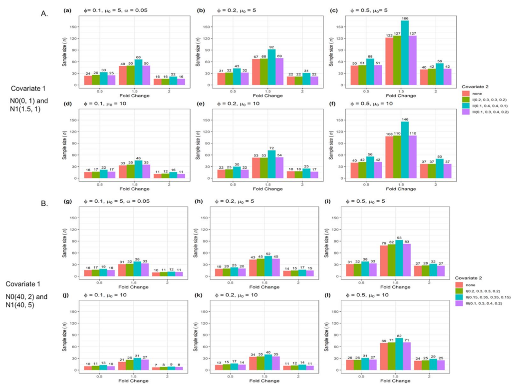
Figure 4 illustrates the n adjusted by two confounders. In the upper panel A (af), a larger n in cyan is observed for the confounding variable N 0 (0, 1) and N 1 (1.5, 1) combined with the high disproportion covariate of II(0.1, 0.4, 0.4, 0.1). Similarly, a larger n in cyan (the bottom panel B: gl) is observed for N 0 (40, 2 2 ) and N 1 (40,   5 2 ) combined with the high disproportion covariate of II(0.15, 0.35, 0.35, 0.15) compared to I(0.2, 0.3, 0.3, 0.2) and III 0.1 , 0.3 , 0.4 , 0.2 with low disproportion. The two confounding covariates corresponding to the adjusted n from largest to smallest are: { N 0 (0, 1) and N 1 (1.5,1), II(0.1, 0.4, 0.4, 0.1) > { N 0 (0, 1) and N 1 (1.5, 1), II(0.2, 0.3, 0.3, 0.2) or III(0.1, 0.3, 0.4, 0.2)}[5,9] > { N 0 (40, 2 2 ) and N 1 (40,   5 2 ), II(0.15, 0.35, 0.35, 0.15)} > { N 0 (40, 2 2 ) and N 1 (40,   5 2 ), II(0.2, 0.3, 0.3, 0.2) or III(0.1, 0.3, 0.4, 0.2)}. While compared to the results from the single confounding variable in Figure 1, Figure 2 and Figure 3, we observed a larger n is required for adjusting two confounding variables such as N 0 (0, 1) and N 1 (1.5, 1) combined with I(0.15, 0.35, 0.35, 0.15) or II(0.1, 0.4, 0.4, 0.1). However, there is no significant difference in the n for the covariate with equal mean (e.g., ( N 0 (40, 2 2 ) and N 1 (40,   5 2 )) combined with a categorical covariate at smaller disproportion (II(0.2, 0.3, 0.3, 0.2) and III(0.1, 0.3, 0.4, 0.2)).

3.3. The n and Actual Power for Testing Multiple Genes

The objective is to calculate the n and actual power for testing multiple genes via rejecting at least one null hypothesis when given a set of genes. In this simulation, the total number of genes per sample T is set to be 10000, true positive genes (DEGs) T 1 is set to be 200. Thus, we have the number of true negative t 0 = T T 1 , which is the number of genes that are not differentially expressed under H 0 . The expected number of true DEGs for a desired power 0.80 is t 1 = 160 . The rest of the parameters, including µ 0 , w, ρ   and   ϕ , remain the same as in testing a single gene. Thus, a significance level α *   in the Equation (6) is calculated as 0.000859, given a nominal FDR   f = 0.05 .
For each combination of these parameter settings, the n is calculated when the observed power is close to the nominal power of 0.80. The gene between two treatment groups for the multiple corrections is considered to be significantly different only when a p-value is   α * 2 = 0.000043 using a two-sided test. The actual power is imputed as the percentage of the number of times that the null hypothesis is rejected at the significance level α * / 2 in the 1000 simulated dataset. Results for each combination of the desired parameters are described below.
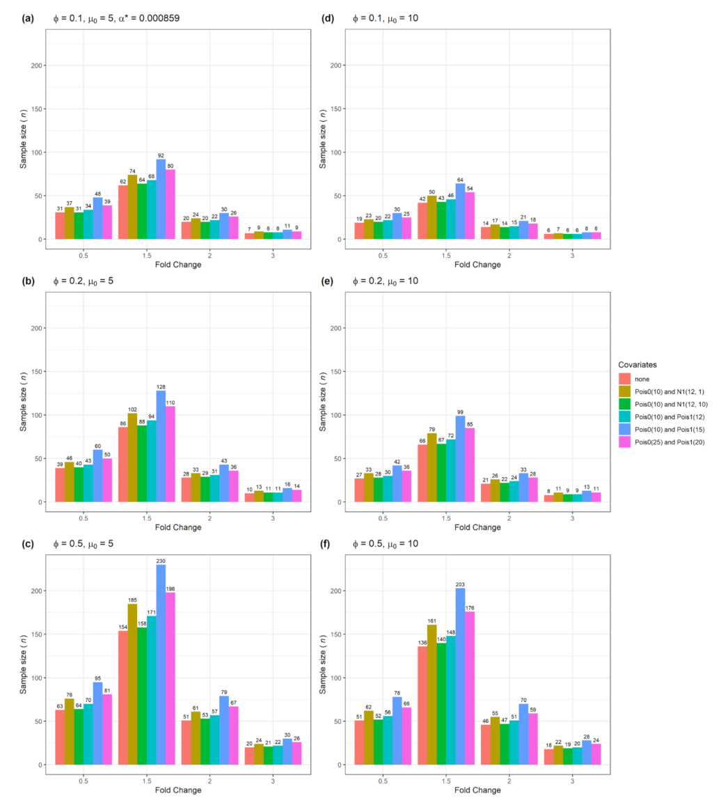
Figure 5, Figure 6, Figure 7 and Figure 8 list the n for testing multiple genes in combinational settings corresponding to Figure 1, Figure 2, Figure 3 and Figure 4 for testing a single gene, respectively. The confounding covariates in Figure 5 and Figure 6 are continuous variables following either a normal or Poisson distribution. The confounder in Figure 7 is a categorical covariate. The sample sizes in Figure 8 are obtained by adjusting two confounding variables. We observed that the pattern of the n changed from different combinations of µ 0 , ϕ and ρ in Figure 5, Figure 6, Figure 7 and Figure 8 is similar to the one observed in Figure 1, Figure 2, Figure 3 and Figure 4. However, given the similar setting, a much larger n for each group is required to achieve the desired power of 0.80 with α * when testing multiple genes compared to a single gene.

3.4. An Example Using COAD RNA-seq Data

We used a colon adenocarcinoma (COAD) data set to illustrate how to calculate sample sizes that are adjusted by age, sex or both in the case of testing multiple genes. The mapped raw reads with 20,531 genes and 500 samples from the file (COAD.mRNAseq_raw_counts.txt) and corresponding clinical matrix data with 459 samples and 3222 covariates from the file (COAD.clin.merged.txt) were downloaded from the Broad GDAC Firehouse on 22 January 2020 (https://gdac.broadinstitute.org). The COAD data file was used in this study is provided (Supplementary File S1).
With the aid of R scripts, we extracted 359 COAD and 41 uninvolved tissue samples that were adjacent to the COAD primary tumors called the normal group in this study. The age and sex for these samples are matched using the COAD.clin.merge.txt file. The genes with more than 60% zero counts across all the samples in both groups and the mean counts across the sample fewer than five were filtered out. A total of 16682 genes remained for downstream analysis. We used the edgeR package to perform the analysis [12]. Briefly, the raw read counts with 500 samples containing 16682 genes were loaded into edgeR for estimating common dispersion and normalization factors (size factor). The TMM (trimmed-mean M value) normalization method from edgeR was used to estimate the size factor. The ratio of the size factor (w) between the normal and COAD groups is 1.05. The estimated common dispersion ϕ is approximately 0.53 [11].
For the confounding covariate age, we estimated the sample mean and variance using the TMM normalized data for the normal and COAD groups. The mean age in the normal and COAD groups is 70.34 and 66.88 years, respectively. The standard deviation of age in the normal and COAD groups is 13.23 and 13.1 years, respectively. Thus, we set age as N 0 (70, 13 2 ).) and N 1 (67,   13 2 ). For the categorical covariate sex, the proportion of males and females in the normal group is 0.24 and 0.26, respectively, while the proportion of males and females in the COAD is 0.26 and 0.24, respectively. Thus, we set sex as VII (0.24, 0.26, 0.26, 0.24) for sample size estimation.
We assumed that the top 500 of 16682 genes are likely prognostic genes (DEGs) and have the largest FC for up or down-regulated genes. The sample size was estimated by setting the mean counts in the control group to be µ 0 = 2 ,   5   and   10 for the genes in different scenarios. In this study, the nominal power is set to be 0.80, which indicates that 400 or more out of the 500 differentially expressed genes (DEGs) will be detected. Given the FDR at f = 0.05 and a 0.80 nominal power, we set T = 16682 ,   T 1 = 500 ,   t 0 = T T 1 and t 1 = 400   ( the expected DEG). The FC is set to be ρ g = 0.5 ,   1.5   and   2 with ϕ   0.53 . With these settings, the new alpha α * = 0.0013 is obtained from the formula (5) at a desired t 1 = 400 . Finally, the n and actual power are estimated using α * / 2 and a nominal power 0.80 (Table 2).
Table 2 reports sample size n in the control and the COAD groups with and without covariate-adjusted by the age, sex and both while assuming 500 DEGs. For the 2 FC of down-regulated genes at ρ = 0.5, the minimum n for the case of non-adjustment is 107, given the minimum mean reads of the gene in the control group µ 0 = 2 . As the µ 0 increases to 5 and 10, the n decreases to 71 and 59, respectively. We observed that the n adjusted by the age or sex and both variables is slightly larger than that of non-adjustment in some of the settings. However, the samples size n adjusted by both of age and sex is slightly larger than non-adjustment for all the settings. Similar results are observed for upregulated genes with ρ = 1.5 and 2. This indicates that age and sex could be the potential confounding variables in the COAD RNA-seq data.

4. Discussion

In this study, we performed both non-covariate and covariate-adjusted sample size and power calculations using simulated data as well as a real dataset. Taking the confounding covariates into consideration is an extension of our previous work [4,5]. This approach is an advancement over the current methods for sample size calculation in designing RNA-seq experiments [1,2,3,6,7,8,13,14]. Based on our knowledge, currently, there are no existing methods for calculating sample sizes by adjusting confounding covariates for buck RNA-seq experimental design. Therefore, there are no benchmark comparisons in our study. More importantly, our simulation-based method for estimating sample size and power described here is quite flexible and very useful to apply in both basic science and clinical science RNA-seq data.
In performing the simulation studies, we considered different scenarios for the confounding covariates with a different data type and distribution. We found that a large sample size is required to achieve the desired 80% detection power when the heterogeneous confounding variables exist. Without consideration of cofounding covariates, the sample size obtained by the methods will likely be underestimated. Consequently, the power for detecting the DEGs will probably be below the desired power of 0.8.
Similarly, we used a two-sided statistical test for the model parameter ψ 1 from a standard GLM to estimate sample size and power, which are based on the DEG analysis in RNA-seq data [5]. We have incorporated a common dispersion parameter, the size factor and confounding covariates via a log link function using an NB regression model, which is extended from the previous study [23].
Most importantly, in this paper, sample size calculation methods are presented under a wide range of settings for accommodating confounding covariates denoted by a continuous [24], a categorical variable [22] or both. The actual power in this study is very close to or higher than the nominal power of 0.80 for all the settings. The results indicate the required sample size is larger given additional heterogeneity in the data, which needs to be addressed in RNA-seq studies.
In the simulation study, we arbitrarily chose µ 0 = 5 as a minimum read in control group of DEGs, which is commonly used as a cutoff to filter out lowly expressed genes in RNA-seq analysis. For a low µ 0 , a study requires a large n to achieve a nominal power at 80% or higher, which may not be feasible in practice due to the cost. As an alternative, a higher read depth sequencing may be chosen to increase the mean read counts for each sample instead of directly increasing the sample size, as is shown in Lamarre et al. [25]. In current simulations, µ 0 parameters are simply fixed as 5 and 10. For the real dataset, µ 0 varies with sequencing read depth and experimental conditions. For differentially and highly expressed genes in an experiment, the µ 0 could be chosen to be larger than 5 or 10 or vice versa. Moreover, when testing multiple genes in the simulation, we arbitrarily chose 10000 genes with 200 true DEGs (Figure 5, Figure 6, Figure 7 and Figure 8). In reality, the total number of detected genes could vary depending upon the read depth in each sequencing sample and experimental conditions. In this example analysis, we demonstrate that the sample size is calculated based on the number of genes and parameters that are estimated from real RNA-seq data. Due to the large sample size from COAD data, we set 500 true DEGs to estimate the sample size with a desired power. Currently, the number of DEGs identified by the common RNA-seq analysis tools is varied due to high false-positive rates [18]. Determining the true number of DEGs is usually objective by researchers because it depends on the tools and the cutoff value of fold change and adjusted p-value that are chosen. Finally, in this study, we focused on the equal read depth due to improvements in RNA-seq technology and library preparation. We also focused on a balanced experimental design for the simulation study.

5. Conclusions

In summary, the methods described here illustrate how to estimate sample size when confounding variables are likely to exist in any complex RNA-seq experimental design. We observed that a larger sample size is required for the likely presence of single or multiple confounding variables in order to achieve a nominal power of 0.80. The results provide investigators with a variety of choices for the sample size that might be required for designing their experiments. Most importantly, when a confounding covariate with a known distribution exists in an experiment, one should incorporate such information into sample size calculation.

Supplementary Materials

The following are available online at https://www.mdpi.com/article/10.3390/biomedinformatics1020004/s1: File S1: R source codes for the simulation study with detailed explanations are provided. File S1 R codes in PDF format illustrate how to estimate sample size and power for testing a single gene for Figure 1 and multiple genes for Figure 5 given FC = 2 and other parameters in the presence of confounding covariates. File S2: Datasets used for the analysis. This zipped file folder contains COAD raw reads of 500 samples (COAd.uncv2.mRNAseq_raw_counts.txt).

Author Contributions

Conceptualization, X.L. and S.N.R.; formal analysis, X.L.; methodology, X.L.; software, X.L.; writing—original draft preparation, X.L. and T.E.O.; writing—review and editing, T.E.O., S.N.R., E.C.R. and N.G.F.C.; supervision, E.C.R. and N.G.F.C.; funding acquisition, N.G.F.C. All authors have read and agreed to the published version of the manuscript.

Funding

This research was supported by the National Institutes of Health grant, P20GM103436.

Data Availability Statement

The R code and datasets used in this study are available (Additional File S1 and File S2), respectively.

Acknowledgments

The authors gratefully thank the reviewers for the very good suggestions, advice and comments.

Conflicts of Interest

The authors declare no conflict interests.

References

  1. Fang, Z.; Cui, X. Design and validation issues in RNA-seq experiments. Brief. Bioinform. 2011, 12, 280–287. [Google Scholar] [CrossRef] [Green Version]
  2. Li, C.I.; Su, P.F.; Guo, Y.; Shyr, Y. Sample size calculation for differential expression analysis of RNA-seq data under Poisson distribution. Int. J. Comput. Biol. Drug Des. 2013, 6, 358–375. [Google Scholar] [CrossRef] [PubMed]
  3. Li, C.I.; Su, P.F.; Shyr, Y. Sample size calculation based on exact test for assessing differential expression analysis in RNA-seq data. BMC Bioinform. 2013, 14, 357. [Google Scholar] [CrossRef] [Green Version]
  4. Li, X.; Cooper, G.F.; Shyr, Y.; Wu, D.; Rouchka, E.C.; Gill, R.S.; O’Toole, T.E.; Brock, G.N.; Rai, S.N. Inference and Sample Size Calculations Based on Statistical Tests in a Negativ ebnomial Distribution for Differential Gene Expression in RNA-seq Data. J Biom. Biostat. 2017, 8. [Google Scholar] [CrossRef] [Green Version]
  5. Li, X.; Wu, D.; Cooper, N.G.F.; Rai, S.N. Sample size calculations for the differential expression analysis of RNA-seq data using a negative binomial regression model. Stat. Appl. Genet. Mol. Biol. 2019, 18. [Google Scholar] [CrossRef] [PubMed]
  6. Ching, T.; Huang, S.; Garmire, L.X. Power analysis and sample size estimation for RNA-Seq differential expression. RNA 2014, 20, 1684–1696. [Google Scholar] [CrossRef] [Green Version]
  7. Hart, S.N.; Therneau, T.M.; Zhang, Y.; Poland, G.A.; Kocher, J.P. Calculating sample size estimates for RNA sequencing data. J. Comput. Biol. 2013, 20, 970–978. [Google Scholar] [CrossRef] [Green Version]
  8. Liu, Y.; Zhou, J.; White, K.P. RNA-seq differential expression studies: More sequence or more replication? Bioinformatics 2014, 30, 301–304. [Google Scholar] [CrossRef]
  9. Yu, L.; Fernandez, S.; Brock, G. Power analysis for RNA-Seq differential expression studies. BMC Bioinform. 2017, 18, 234. [Google Scholar] [CrossRef]
  10. Anders, S.; Huber, W. Differential expression analysis for sequence count data. Genome Biol. 2010, 11, R106. [Google Scholar] [CrossRef] [Green Version]
  11. Robinson, M.D.; Smyth, G.K. Small-sample estimation of negative binomial dispersion, with applications to SAGE data. Biostatistics 2008, 9, 321–332. [Google Scholar] [CrossRef] [Green Version]
  12. Robinson, M.D.; McCarthy, D.J.; Smyth, G.K. edgeR: A Bioconductor package for differential expression analysis of digital gene expression data. Bioinformatics 2010, 26, 139–140. [Google Scholar] [CrossRef] [PubMed] [Green Version]
  13. Zhao, S.; Li, C.I.; Guo, Y.; Sheng, Q.; Shyr, Y. RnaSeqSampleSize: Real data based sample size estimation for RNA sequencing. BMC Bioinform. 2018, 19, 191. [Google Scholar] [CrossRef]
  14. Wu, H.; Wang, C.; Wu, Z. PROPER: Comprehensive power evaluation for differential expression using RNA-seq. Bioinformatics 2015, 31, 233–241. [Google Scholar] [CrossRef] [PubMed] [Green Version]
  15. Dillies, M.A.; Rau, A.; Aubert, J.; Hennequet-Antier, C.; Jeanmougin, M.; Servant, N.; Keime, C.; Marot, G.; Castel, D.; Estelle, J.; et al. A comprehensive evaluation of normalization methods for Illumina high-throughput RNA sequencing data analysis. Brief. Bioinform. 2013, 14, 671–683. [Google Scholar] [CrossRef] [Green Version]
  16. Kvam, V.M.; Liu, P.; Si, Y. A comparison of statistical methods for detecting differentially expressed genes from RNA-seq data. Am. J. Bot. 2012, 99, 248–256. [Google Scholar] [CrossRef] [Green Version]
  17. Li, X.; Brock, G.N.; Rouchka, E.C.; Cooper, N.G.F.; Wu, D.; O’Toole, T.E.; Gill, R.S.; Eteleeb, A.M.; O’Brien, L.; Rai, S.N. A comparison of per sample global scaling and per gene normalization methods for differential expression analysis of RNA-seq data. PLoS ONE 2017, 12, e0176185. [Google Scholar] [CrossRef]
  18. Li, X.; Cooper, N.G.F.; O’Toole, T.E.; Rouchka, E.C. Choice of library size normalization and statistical methods for differential gene expression analysis in balanced two-group comparisons for RNA-seq studies. BMC Genom. 2020, 21, 75. [Google Scholar] [CrossRef] [PubMed]
  19. Lund, S.P.; Nettleton, D.; McCarthy, D.J.; Smyth, G.K. Detecting differential expression in RNA-sequence data using quasi-likelihood with shrunken dispersion estimates. Stat. Appl. Genet. Mol. Biol. 2012, 11. [Google Scholar] [CrossRef]
  20. Seyednasrollah, F.; Laiho, A.; Elo, L.L. Comparison of software packages for detecting differential expression in RNA-seq studies. Brief. Bioinform. 2015, 16, 59–70. [Google Scholar] [CrossRef] [PubMed] [Green Version]
  21. Nelder, J.A.; Wedderburn, R.W.M. Generalized linear model. J. R. Stat. Soc. 1972, 135, 370–384. [Google Scholar] [CrossRef]
  22. Self, S.G.; Mauritsen, R.H. Power Sample-Size Calculations for Generalized Linear-Models. Biometrics 1988, 44, 79–86. [Google Scholar] [CrossRef]
  23. Zhu, H.; Lakkis, H. Sample size calculation for comparing two negative binomial rates. Stat. Med. 2014, 33, 376–387. [Google Scholar] [CrossRef] [PubMed]
  24. Shieh, G. On power and sample size calculations for likelihood ratio tests in generalized linear models. Biometrics 2000, 56, 1192–1196. [Google Scholar] [CrossRef]
  25. Lamarre, S.; Frasse, P.; Zouine, M.; Labourdette, D.; Sainderichin, E.; Hu, G.; Le Berre-Anton, V.; Bouzayen, M.; Maza, E. Optimization of an RNA-Seq Differential Gene Expression Analysis Depending on Biological Replicate Number and Library Size. Front. Plant Sci. 2018, 9, 108. [Google Scholar] [CrossRef] [PubMed] [Green Version]
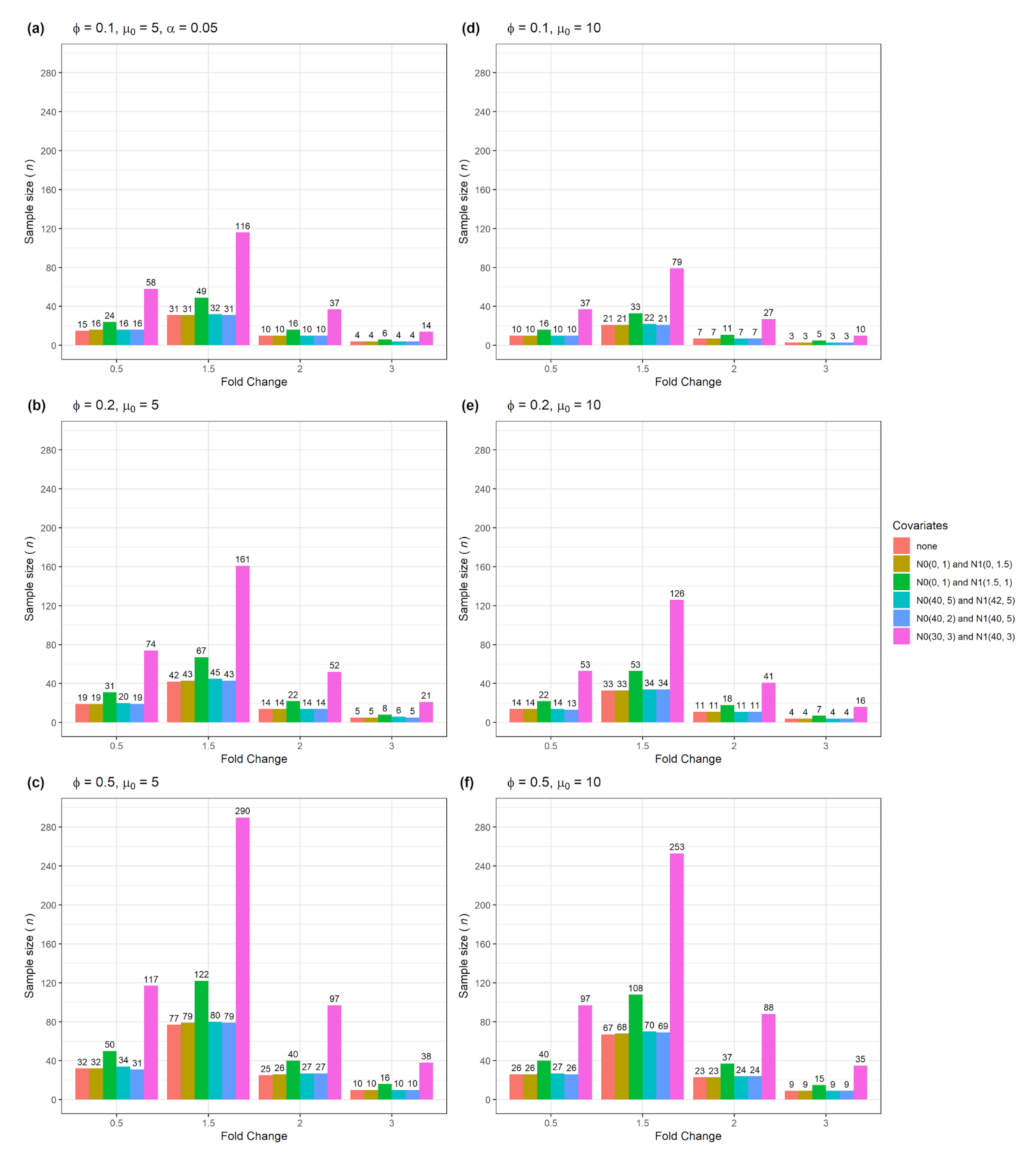
Figure 1. Calculated sample size n and actual power adjusted by a confounder with a normal distribution. The color-coded bars represent covariates, and the height of the bars represents the sample size given α for testing a single gene. (ac) shows n vs. fold change ρ given dispersion ϕ (0.1, 0.2, 0.5) and mean counts in control µ 0 = 5. (df) shows n vs. ρ given ϕ (0.1, 0.2, 0.5) and µ 0 = 10.
Biomedinformatics 01 00004 g001
Figure 2. Calculated sample size n and actual power adjusted by a confounder with a Poisson distribution or a mixture of normal and Poisson distribution. The color-coded bars represent confounding covariates, and the height of the bars represents n given α for testing a single gene. (ac) shows n vs. ρ given ϕ (0.1, 0.2, 0.5) and µ 0 = 5. (df) shows n vs. ρ given ϕ (0.1, 0.2, 0.5) and µ 0 = 10.
Biomedinformatics 01 00004 g002
Figure 3. Calculated sample size n and actual power adjusted by a categorical confounder. The color-coded bars represent confounding covariates, and the height of the bars represents n given α for testing a single gene. (ac) shows n vs. ρ given ϕ (0.1, 0.2, 0.5) and µ 0 = 5. (df) shows n vs. ρ given ϕ (0.1, 0.2, 0.5) and µ 0 = 10.
Biomedinformatics 01 00004 g003
Figure 4. Calculated sample size n adjusted by two confounders. The color-coded bars represent categorical confounders (Covariate 2), and the height of the bars represents n given α for testing a single gene. The confounder (Covariate 1) in panel A (af) has a normal distribution: N 0 (0, 1) and N 1 (1.5, 1). The confounder (Covariate 1) in panel B (gl) has a normal distribution: N 0 (40, 5 2 ) and N 1 (42, 5 2 ).
Biomedinformatics 01 00004 g004
Figure 5. Calculated sample size n adjusted by a confounder in a normal distribution. The color-coded bars represent confounding covariates, and the height of the bars represents n given α* for testing 10000 genes. (ac) shows n vs. fold change ρ given dispersion ϕ (0.1, 0.2, 0.5) and mean counts in control µ 0 = 5. (df) shows n vs. ρ given ϕ (0.1, 0.2, 0.5) and µ 0 = 10.
Biomedinformatics 01 00004 g005
Figure 6. Calculated sample size n adjusted a confounder in a Poisson distribution or a mix of normal and Poisson distribution. The color-coded bars represent confounding covariates, and the height of the bars represents n given α* for testing 10000 genes. (a–c) shows n vs. fold change ρ given dispersion ϕ (0.1, 0.2, 0.5) and mean counts in control µ 0 = 5. (df) shows n vs. ρ given ϕ (0.1, 0.2, 0.5) and µ 0 = 10.
Biomedinformatics 01 00004 g006
Figure 7. Calculated sample size n adjusted by a categorical confounder. The color-coded bars represent confounding covariates, and the height of the bars represents n given α*. (ac) shows n vs. ρ given ϕ (0.1, 0.2, 0.5) and µ 0 = 5. (df) shows n vs. ρ given ϕ (0.1, 0.2, 0.5) and µ 0 = 10 for testing 10000 genes.
Biomedinformatics 01 00004 g007
Figure 8. Calculated sample size n adjusted by two confounders. The color-coded bars represent categorical confounders (Covariate 2), and the height of the bar graph represents the n given α* for testing 10000 genes. The confounder (Covariate 1) in the panel A (af) has a normal distribution: N 0 (0, 1) and N 1 (1.5, 1). The confounder (Covariate 1) in the panel B (gl) has a normal distribution: N 0 (40, 5 2 ) and N 1 (42,   5 2 ).
Biomedinformatics 01 00004 g008
Table 1. A summary of the simulation characteristics for the sample size calculation illustrated in Figure 1, Figure 2, Figure 3, Figure 4, Figure 5, Figure 6, Figure 7 and Figure 8.
FigureSingle Gene Multiple GenesNumber of ConfoundersData Type
Figure 1YesNo1Numerical with normal distribution
Figure 2YesNo1Numerical with normal or Poisson distribution
Figure 3YesNo1Categorical
Figure 4YesNo2Numerical and categorical data
Figure 5NoYes1Numerical with normal distribution
Figure 6NoYes1Numerical with normal or Poisson distribution
Figure 7NoYes1Categorical
Figure 8NoYes2Numerical and categorical
The parameter settings are ϕ (dispersion) = (0.1, 0.2, 0.5),   µ 0 (mean read counts of control) = (5, 10),ρ(fold change) = (0.5, 1.5, 2, 3), α (type I error rate) = 0.05, α * adjusted   α = 0.000859 and a nominal power at 0.8.
Table 2. The calculated sample size n and estimates of power from COAD data.
ρ µ 0 No confoundersAge
N 0 ( 70 ,   13 )   and   N 1 ( 67 , 13 )
Sex
VII(0.24, 0.26, 0.26, 0.24)
Age and Sex
nPower
(%)
nPower
(%)
nPower
(%)
nPower
(%)
0.5210780.210880.110780.210980.26
57180.27380.67280.57380.52
105980.85980.15980.66080.90
1.5216580.316880.516680.416880.34
512480.6212580.0812480.6412580.5
1010780.410980.1610880.2810980.26
226080.96080.06080.86180.58
54480.24580.64581.34580.6
104080.74180.84080.64180.46
Shown are n and actual power adjusted by the confounders of age and sex variables given nominal power of 0.8 with FDR 0.05, the ratio of size factor w = 1.05 ,   dispersion   ϕ = 0.53   and   adjusted   size   α * = 0.0013.
Publisher’s Note: MDPI stays neutral with regard to jurisdictional claims in published maps and institutional affiliations.