Developing Correction Methods for New Fibrogram-Based Length Measurements

Abstract

Cotton fiber length is a key determinant of yarn quality, and High Volume Instrument (HVI) measurements are widely used to assess fiber length characteristics. Recent research has shown that the complete HVI fibrogram contains substantially more information than the conventional HVI-reported parameters, enabling reconstruction of the full fiber-length distribution and calculation of additional length-related parameters. Before these measurements can be adopted for routine use, calibration procedures are needed to ensure agreement among instruments. This study developed and evaluated calibration procedures for fibrogram-derived length parameters calculated from reconstructed fiber-length distributions. Three calibration reference cottons representing short, medium, and long fiber lengths were established and tested on four HVIs over a six-month period. Calibration equations were generated using two-point and three-point linear regressions between reference and observed measurements and applied to USDA evaluation cottons and commercial samples. Instrument stability, calibration frequency, and the use of comb checks were also investigated. Stability analysis showed that measurement drift within individual HVIs was small over the study period, indicating that frequent calibration is unnecessary under well-maintained operating conditions. Calibration improved agreement among HVIs for both conventional HVI-reported parameters and fibrogram-derived length parameters. Two-point and three-point calibration produced similar results, suggesting limited benefit from the additional medium-length calibration standard. Calibration frequency and comb checks had minimal impact on calibration efficacy. Overall, the proposed procedures improve consistency among HVIs and support practical implementation of new fibrogram-derived length measurements.

1. Introduction

Cotton fiber quality parameters are essential in assessing the spinnability of cotton lint into yarn [1,2]. Among these parameters, fiber length properties function as the main contributor to yarn strength and performance [3,4,5]. In particular, fibers must have sufficient length and strength to withstand mechanical stress during spinning and to effectively contribute to yarn formation. For example, in ring spinning, long staple fibers have a greater chance to contribute to the twist zone of yarn and therefore have a greater effect on yarn strength [6]. In addition, fiber-length characteristics are particularly important for modern air-jet (vortex) spinning systems, where adequate fiber length and length uniformity are required to ensure efficient fiber control, yarn formation, and acceptable yarn strength [7].

However, the extent of this contribution depends on the natural variability in cotton fiber length, which exists across a single seed, within a boll, and among the positions of the bolls on a cotton plant [8,9]. The maximum fiber length can be found before weathering and harvesting. This variation in the cotton fiber length increases as the fibers undergo further processing, such as ginning. Given that a single bale of cotton may contain about 50 billion individual fibers [10], the resulting distribution of the fiber qualities within a cotton bale becomes highly heterogeneous. This distribution significantly affects spinning performance and, hence, yarn quality [11].

Consequently, accurate characterization of fiber properties becomes essential. In the cotton industry, two main approaches are implemented to determine fiber quality: bundle testing and individual fiber testing [12]. Between them, bundle testing is the most common technique for evaluating fiber quality, and it can be conducted faster than individual fiber testing. Moreover, fiber bundles are logically related to yarn since a yarn is a twisted bundle of fibers. However, for a more thorough characterization of fiber quality, individual fiber testing may be needed.

The most common instrument for bundle fiber testing is the USTER High Volume Instrument (HVI) (USTER Technologies, Memphis, TN, USA). It is a series of fiber-quality testing instruments integrated into a single measurement system. The HVI can measure micronaire, length, strength, color, and trash in approximately 30 s [13,14]. The speed of the HVI is one of the main benefits for the United States Department of Agriculture (USDA) Agricultural Marketing System (AMS), which classes more than 15 million bales of U.S. cotton annually. Likewise, cotton breeding programs rely extensively on HVI measurements because the rapid testing process enables the economical evaluation of large numbers of breeding lines. Furthermore, HVI-based fiber quality parameters are of particular importance because they constitute the primary quality attributes used within the U.S. cotton marketing system.

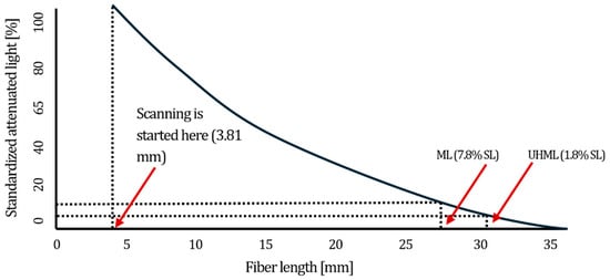
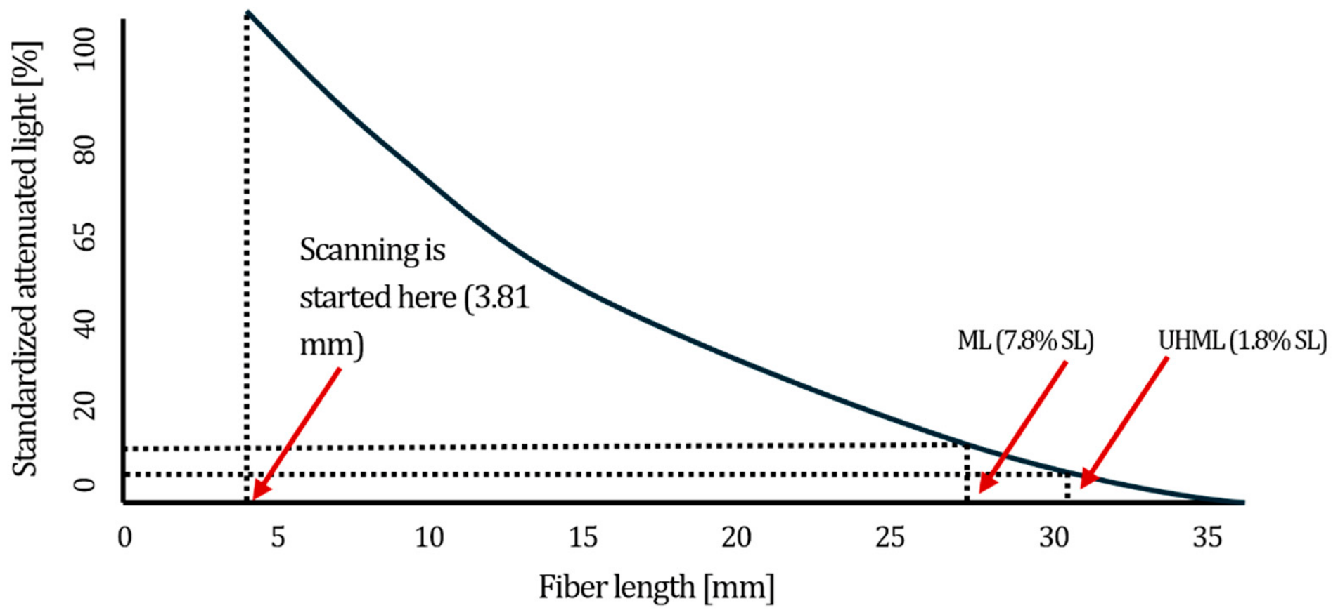
For measuring fiber length with the HVI, approximately 10 g of cotton fiber is placed into a rotating drum, where mechanical fingers convey the sample toward the perforated portion of the drum. As the drum rotates, a comb with needles collects fibers from the sample to form a fiber beard. The resulting fiber beard contains approximately 15,000–20,000 fibers [13,14]. Subsequently, a brushing mechanism removes loosely attached and extraneous fibers from the beard, thereby reducing the influence of fiber crimp on the measurement. Upon completion of the brushing process, the fiber beard is inserted into a narrow slit equipped with a row of light-emitting diodes (LEDs) beneath the sample and a corresponding row of photodiodes above the sample. The system then scans the fiber beard and records light attenuation as a function of distance along the beard, beginning at 3.81 mm (0.15 in) from the comb and extending to the tips of the longest fibers [15]. The HVI normalizes the measured signal by assigning the initial scanning position near the comb as the point of maximum light attenuation (100%). As the scanning position progresses toward the tip of the fiber beard, the number of fibers intercepting the light decreases, resulting in progressively lower attenuation values until the end of the beard, corresponding to 0% attenuation, is reached. From the resulting fibrogram, the HVI calculates upper half mean length (UHML) and mean length (ML) and reports UHML together with the uniformity index (UI = ML/UHML × 100%).

While HVI is the most commonly used tool by breeders, the USTER Advanced Fiber Information System (AFIS) is an alternative measurement system that provides more detailed fiber quality information than the HVI. With this instrument, a 0.5-g hand-crafted sliver is fed through a series of belts and rollers into an individualizer. It contains a rotor covered with metal teeth that individualizes the fibers and removes the trash [16,17]. The individualized fibers are drawn into an airstream, while an electro-optical sensor measures the length (3000 to 5000 individual fibers), maturity, and fineness of each fiber [18,19,20]. This method enables the AFIS to produce a complete fiber length distribution, from which any number of length statistics can be calculated. Because yarn formation is influenced by the entire fiber-length population rather than a single average length measure, access to complete fiber-length distribution information may provide a more comprehensive characterization of cotton fiber quality by capturing variations in the long-fiber and short-fiber fractions within a cotton sample [12,21]. However, a single repetition of 3000 fibers takes about 2–3 min to complete [22,23]. The increased testing time, along with the necessity of a trained technician to create the sliver, makes the AFIS a more costly test, typically limiting its use by breeders to only the more promising lines.

To improve the length information obtained from the HVI, researchers have been working to extract more length information from the HVI fibrogram. In 2020, Sayeed et al. showed that the HVI calculates the UHML and ML directly from the 1.8% and 7.8% span lengths, respectively (Figure 1) [14]. A span length is defined as the length of the fibers at a given percentage of light attenuation, in which the light attenuation is meant to represent a percentage of the number of fibers. For example, the 1.8% span length is the distance from the clamp on a fiber beard to a point at which only 1.8% of the fibers extend. Sayeed also demonstrated that these two measurements do not characterize the total length variation captured by the fibrogram but only the variation in the length of the longest fibers within the sample. In 2022, Tesema et al. investigated different parts of the fibrogram using various span lengths [24]. The authors used a set of eight span lengths to analyze the fibrogram stability and reproducibility among HVIs. In their research, the authors found that although fibrogram length values within the same sample are stable over long- and short-term periods, they vary across HVIs. More recently, Turner et al. presented an algorithm to reconstruct the complete fiber-length distribution from an HVI Fibrogram [23]. Using signal processing techniques as well as the fibrogram theory of Chu and Riley [25], the algorithm is able to recover the complete length distribution of the sample, from which one can calculate a variety of length statistics—similar to the AFIS.

Each of the methods proposed by Sayeed et al., Tesema et al., and Turner et al. provides a new way to obtain additional length information based on the HVI fibrogram principle. However, as both Sayeed and Tesema discussed, fibrogram measurements may differ among HVIs for the same sample. Therefore, it is necessary to apply a correction to the new measurements to ensure they align more closely with a common reference. Both authors described different approaches to this process. Additionally, it should be noted that while this process is technically a correction, with the HVI, it is commonly referred to as calibration in the industry. For the sake of consistency, we will continue to use that terminology in this study.

Calibration is a fundamental requirement for scientific measurement instruments because it ensures that instrument outputs are traceable to accepted reference values. Due to sensor drift, mechanical wear, aging of instrument components, and other sources of systematic error, measurement results may change over time [26]. Even when measurements remain stable within an individual instrument, other instruments of the same type may produce different results for identical samples because of instrument-to-instrument variation. Furthermore, the rate and magnitude of sensor and mechanical drift may vary among instruments, leading to increasing measurement discrepancies over time. For most measurement systems, calibration is performed using a stable reference standard with known properties. For example, weighing devices are calibrated using certified standard masses, whereas pH meters are calibrated using buffer solutions of known pH values. Calibration of the HVI, however, presents unique challenges. Unlike many measurement systems, the calibration reference for the HVI is cotton fiber rather than a fixed physical standard. Cotton fiber is a biological material that exhibits inherent variability both among and within samples. As noted previously, considerable variation in fiber quality characteristics may occur even among fibers originating from the same cotton boll [9]. Although calibration against an invariant reference material would be preferable, establishing such a reference would require substantial modifications to the current HVI measurement methodology. The development of such an approach is beyond the scope of the present study.

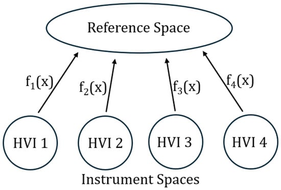
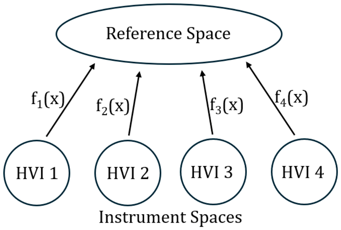
Before discussing calibration methods proposed by Sayeed and Tesema, we will begin with a description of the current HVI calibration process as a point of reference. HVI length calibration utilizes two reference cotton samples: a long and a short cotton sample, which can be obtained from the USDA-AMS. First, each sample is tested with 12 repetitions. These 12 repetitions are then evaluated for outliers—a process that the HVI calls a comb check. If any of the 12 repetitions for each sample is outside of the mean value plus or minus a tolerance value, called a comb check tolerance, that repetition is discarded. After the comb check, if there are fewer than 10 repetitions remaining for either sample, the process starts over by obtaining a new set of 12 repetitions. After the comb check is passed, a linear equation is calculated based on the mean of the observed values (the 10–12 repetitions from each sample) and the reference values using a simple two-point linear regression. Ideally, this equation serves to transform “uncalibrated” instrument values to a common reference space, thereby bringing measurements among HVIs into better agreement. This concept is visually described in Figure 2. In this figure, each High Volume Instrument (HVI) operates within its own instrument measurement space and may produce slightly different values for the same cotton sample due to instrument-specific biases and variability. These calibration functions, denoted as f1(x), f2(x), f3(x), and f4(x), developed for each HVI using reference cotton standards and are applied to transform measurements to a common reference scale. This process enables measurements from different HVIs to be directly compared and improves consistency and agreement across instruments.

Regarding the aforementioned works of Sayeed and Tesema, they also explored the issue of calibration for their methods. In 2022, Sayeed et al. proposed a correction method for the entire fibrogram [27]. In that study, the authors tested nine samples across three HVIs. They selected one of the HVIs as the reference HVI arbitrarily, as there is no established reference for other measurements based on the fibrogram (except for the ones currently used by the HVI). Using principal component analysis (PCA), the authors converted the fibrogram into three principal components. Then they used linear regression to align the principal components of the reference HVI with the other two test HVIs. The fibrograms were then reconstructed through the use of the reference PCA loadings. The authors validated their method using the Euclidean distance between the corrected and reference fibrograms. In a different approach, Tesema et al. developed correction equations to reduce differences among four different HVIs [24]. The authors followed a process similar to the calibration process currently employed for the HVI. However, instead of UHML (1.8% span length) and ML (7.8% span length), they corrected eight span lengths (2%, 8%, 15%, 25%, 40%, 50%, 60%, 75%). To establish the reference measurement for developing the calibration equations, they used two USDA length calibration cotton standards (the same two used in the calibration of the HVI) and tested them for 100 repetitions with two HVIs and averaged them. Similar to the HVI calibration process, they tested these two samples with 12 repetitions each on four HVIs. Simple linear regression between the reference and the average of 12 repetitions (observed values) was used to generate correction equations for a series of span lengths for each HVI. The authors applied these correction equations to 13 USDA evaluation samples. Tesema et al. showed that their correction procedure effectively reduces the level of differences among the multiple HVIs [24].

Previous studies demonstrated that the HVI fibrogram contains substantially more information than the conventionally reported HVI length parameters and that the complete fiber length distribution can be reconstructed from fibrogram data. This advancement enables the calculation of additional length-related parameters. The present study further contributes by developing and evaluating calibration procedures for these fibrogram-derived parameters, thereby improving their consistency across instruments. Although these results represent an important step toward practical implementation, further work is needed to validate the approach across a broader range of cotton types and to establish stronger links between fibrogram-derived parameters and downstream textile performance.

In this paper, we propose a set of calibration methods for new length measurements calculated from the reconstructed distribution of the HVI fibrogram based on Turner’s algorithm [23]. To ensure these new measurements are comparable across instruments, we adopt a calibration strategy inspired by prior work by Tesema, which, as stated, is similar to the current HVI calibration process. By establishing our own reference standard cottons and applying calibration equations derived from these standards, we bring measurements across multiple HVIs into better agreement. This enables the reconstructed length parameters to be used reliably in breeding and commercial contexts. Specifically, in this paper, we make the following contributions:

• Establish three calibration reference standards for long, medium, and short length cottons.
• Establish a method to generate calibration equations using these new reference cottons.
• Conduct stability analysis of the uncalibrated measurements calculated from the reconstructed fiber length distribution.
• Analyze calibration efficacy using the mean absolute difference among HVIs before and after calibration.
• Evaluate whether using comb checks improves calibration efficacy.

2. Materials and Methods

We aim to develop a calibration method to bring uncalibrated measurements into a common reference space in order to improve measurement similarity among HVIs. Calibrating these parameters requires a set of standards. Traditionally, two-point linear regression between the reference and tested measurements is used in HVI to formulate the calibration equations. We sought to determine whether a three-point calibration approach provides improved calibration performance relative to the conventional two-point calibration method used in HVI systems. To facilitate this comparison, three calibration cotton bales were acquired and homogenized through blending to minimize within-sample variability. These materials were subsequently used to establish a set of three reference calibration standards. Experimental data were collected by testing these calibration bales, USDA evaluation samples, and commercial samples with four HVIs at two lab facilities over a period of six months. We developed calibration equations using two-point and three-point linear regression between the reference and observed values of the calibration cottons and applied them to the USDA evaluation and commercial samples. To perform three-point calibration, we would also require reference values of medium-length calibration samples along with the long and short, which are used during traditional two-point calibration. To evaluate the efficacy of our calibration method, we calculated the absolute difference in measurements between uncalibrated and calibrated mean differences among HVIs. Furthermore, we explored the effect of comb checks and HVIs with frequent operational issues on the calibration efficacy. The following sections detail these efforts.

2.1. Calibration Standard Sample Development

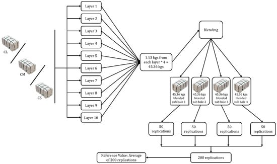
The bales selected to establish the calibration reference measurements were selected because their fiber length parameters best cover the range of current US-produced cotton. To reduce within-bale variability, we blended each bale separately using the following protocol. First, each bale was divided into ten layers, and approximately 1.13 kg (2.5 lbs) of cotton was taken from each layer. This process was repeated four times to fill each of four Hunter 240BFC hoppers with 11.3 kg (25 lbs) of lint (manufacturer details unavailable due to the age of the equipment). For blending, the system was set up to deposit the blended lint at the condenser of the AMH Tuft-O-Matic blender (American Manufacturing & Hydraulics, Camarillo, CA, USA), where it is collected and pressed to form a ~45 kg (~100 lb) blended mini bale. Four blended mini bales were created from each calibration bale in this manner.

To establish reference values for each calibration standard, 50 repetitions of HVI length testing were performed for each of the four blended mini bales, producing 200 repetitions in total for each calibration standard. The summary statistics of the length properties measured in those 200 repetitions are shown in Tables S1, S2 and S3 for calibration long (CL), medium (CM), and short (CS) bales, respectively. The average of the 200 repetitions was then taken as the reference value (for each measurement). In this way, we established three calibration reference measurements for all three reference bales. We should note that the HVI used to produce the reference values was not used in the rest of the experiment. A diagram of this entire process is shown in Figure 3.

2.2. Experimental Data Set

We developed an experimental protocol to collect data over a six-month period, testing the calibration standards (in order to develop and assess calibration equations) as well as samples used to evaluate calibration efficacy. During that time, we tested a set of samples on 30 different days. Hence, we produced 30 sets of samples. Each set was split in half. One-half was tested on two HVIs (labeled as C1 and C2) at Cotton Incorporated in Cary, NC, and the other half on two HVIs (labeled as F1 and F2) at Texas Tech University (TTU) Fiber and Biopolymer Research Institute (FBRI) in Lubbock, TX, USA. One or two sets were tested each week, with at least one day between testing sessions. The labs did not coordinate testing the same sets on the same day, but we aimed to keep both labs generally synchronized. The study was conducted from April to the early part of October 2024.

Our sample set and test protocol for each day’s testing consisted of the following:

• Three Calibration Standards: 24 reps each of the long (CL), medium (CM), and short (CS) standards
• Nine USDA evaluation cottons (EV) (staple lengths 31–38, plus one sample with a staple length of 41); four reps of each
• 16 commercial samples taken from a geographically diverse set of commercial samples drawn from the 2023 US crop (with each set containing a different set of 16 samples); four reps of each

We tested the calibration samples with 24 repetitions, which is twice the number of repetitions required for the current HVI calibration process, as previously mentioned. This choice will be explained later. The USDA evaluation samples are samples that were obtained from the USDA Agricultural Marketing System Cotton and Tobacco Program Cotton Standards office. Staple lengths 31–38 are part of the “8 × 8 Evaluation” cottons, while the staple length 41 cotton is considered by the USDA as a “research bale.” These samples were included in each of the 30 sets to provide a consistent set of samples from a range of lengths each day. Finally, the commercial samples add diversity to the experiment, totaling 480 over the testing duration (16 different samples per day × 30 testing days). All samples were conditioned for at least 48 h at 21 ± 1° C and 65 ± 2% relative humidity prior to testing.

2.3. Stability Analysis

Over time, the mechanical parts of the HVI experience wear and tear, which can lead to measurement drift. This is one of the reasons why calibration is necessary. In order to assess this drift, we conducted a stability analysis over the six-month period on all four HVIs. We used linear regression to assess temporal trends in the measurements and to determine whether significant increases or decreases occurred over the study period. Since this type of analysis can only be performed using the same samples each testing day, we limited the analysis to only the calibration and USDA evaluation samples. Performing a linear regression between the measurements and the number of testing days visually showed whether there was a trend in the data as the time progressed. Furthermore, we evaluated the 95% confidence interval of the slope to examine whether the trend is statistically significant.

2.4. Calibration Method

As our study is concerned with calibrating parameters that are calculated from the reconstructed length distribution acquired from the HVI fibrogram, we followed a similar calibration procedure as is currently employed by HVI. Linear calibration models were used for all parameters. This assumes that inter-instrument differences are approximately linear over the range of observed measurements. This assumption is supported by preliminary scatterplots showing strongly linear relationships between instruments within the calibration ranges considered. Potential nonlinear corrections were not investigated in this study. We performed either two-point or three-point linear regression using the created reference standards. For the two-point calibration, CL and CS were used, and all three standards (CL, CM, and CS) were used for the three-point calibration. Two-point regression does not have any degrees of freedom. However, three-point regression may exhibit lower variability due to having one degree of freedom. In our analysis, we explore the differences in these two methods.

As previously mentioned, we conducted testing on 30 separate days over a six-month period, generating data to develop calibration equations on each day for each length parameter. Although the reconstructed fiber length distribution can be used to calculate numerous fiber-length statistics, the present study focused on the development and evaluation of calibration equations for the following parameters:

▪

UHMLf (upper half mean length calculated from the reconstruction algorithm)

▪

MLf (mean length calculated from the reconstruction algorithm)

▪

LHMLf (lower half mean length calculated from the reconstruction algorithm)

▪

SFCf (short fiber content % calculated from the reconstruction algorithm)

These specific parameters were chosen because of the range of lengths they represent. UHMLf represents the longer fibers in a sample, MLf represents the medium-length fibers, and LHMLf and SFCf represent the shorter fibers. Also, to establish a baseline, we included the analysis on the calibration efficacy of the length parameters that the HVI currently reports:

▪

1.8% SL—referred to as UHML by the HVI

▪

7.8% SL—referred to as ML by the HVI

As calibration is a simple linear transformation ($y=mx+c$), for all measurements except one, we applied this transformation directly to the raw, uncalibrated value. However, because SFCf is a percentage and bounded between 0 and 100%, we first converted the percentage to its decimal equivalent, applied a logit transform, i.e., $\mathrm{l}\mathrm{o}\mathrm{g}(x/(1-x\left)\right)$, applied the correction equation in the logit space, and then transformed the corrected/calibrated value back to a percent, i.e., $100\%/(1+e^{-y})$. The logit transformation changed the range of SFCf from negative infinity to positive infinity, similar to other length parameters, making the logit space more appropriate for applying the linear correction.

2.4.1. Varying the Intervals Between Calibrations

Regarding HVI calibration, a question often arises regarding the frequency of calibration. While the stability analysis addresses this issue by investigating instrument drift, this analysis examines whether calibrating more frequently improves the overall calibration efficacy. To do this, we simulated different intervals between calibrations by applying a specific number of calibration equations to the data of specific days. For example, we applied one calibration equation to days 1–15 and another to days 16–30, simulating an interval of approximately three months between calibrations, given that the data collection process spanned six months. Similarly, we used three equations and five equations to simulate calibration intervals of two months and one month, respectively. As the calibration equations are based on linear regression between the reference and observed measurements of a specific day, some days having equations with larger slopes and intercepts could cause higher corrections to the uncalibrated measurements for those days compared to others. Hence, instead of choosing specific equations, we decided to take a randomized approach. For example, to apply two calibration equations, we created 870 random pairs containing numbers from 1 to 30 (a number represents that specific day’s calibration equation), which provided us with 870 unique pairs of calibration equations. We took the first 100 pairs and applied them to the uncalibrated measurements and then averaged the results. We followed a similar procedure for three and five equations. This randomized approach eliminated the possibility of outliers adversely affecting a specific day’s calibration equation.

2.4.2. Applying Comb Checks

As discussed in the introduction, when applying comb checks, the HVI requests that a new set of 12 repetitions be obtained when fewer than 10 repetitions remain after the comb checks remove outlying observations that exceed the mean plus or minus a comb check tolerance value. However, because we cannot alter the HVI software (software version 3.5.2 Build 87), our software implementation of calibration will be implemented separately. As such, it will be practically infeasible to interact with the technician in the same way the HVI software does if a new set of combs is needed. To avoid the need to obtain a new set, we decided to use all 24 repetitions for the calibration methods. Nevertheless, we explored the impact of removing outlying observations on calibration efficacy, i.e., comb checks. We chose the comb check tolerance for UHMLf based on the current HVI-reported UHML comb check tolerance value (0.635 mm). However, MLf, 1.8%, and 7.8% span length showed average standard deviations that are close to 0.635 mm. Since these parameters have similarity with UHMLf, we decided to use the same tolerance value (0.635 mm) for them. The tolerance values represent the absolute allowable deviations from the average of the 24 repetitions. For example, an average SFCf value of 25% with a tolerance of ±3.5 percentage points corresponds to the acceptance of repetitions in the range of 21.5–28.5%.

Table 1. Different length parameters and their tolerance limit.

Parameter	Tolerance Limit
UHMLf	0.635 mm (0.025 inch)
MLf	0.635 mm (0.025 inch)
LHMLf	0.889 mm (0.035 inch)
SFCf	3.5%
1.8% SL	0.635 mm (0.025 inch)
7.8% SL	0.635 mm (0.025 inch)

shows the tolerance values for different parameters.

2.5. Calibration Efficacy Analysis

To evaluate calibration efficacy, we developed a measure of how close measurements are among HVIs after calibration compared to their values before. We assess calibration efficacy by calculating the absolute difference between the uncalibrated and calibrated mean differences among HVIs.

Let $\mathcal{H}=\left\{F_1,F_2,C_1,C_2\right\}$ denote the set of HVIs and $\mathcal{P}=\left\{\left(a,b\right):a,b\in \mathcal{H},a\ne b\right\}$ be a set of unique pairs of HVIs. Since four HVIs were included in the study, there are six unique pairwise comparisons (F1-F2, F1-C1, F1-C2, F2-C1, F2-C2, and C1-C2). Then, the mean absolute differences among pairs of HVIs can be calculated as

$$MAD={\displaystyle \frac{1}{6}}\sum _{(a,b)\in \mathcal{P}}\left|a-b\right|.$$

(1)

Then, let ${MAD}_U$ be the mean absolute deviation among HVIs before calibration (uncalibrated) and ${MAD}_C$ be the mean absolute deviation among HVIs after calibration. We assess calibration efficacy by

$$D={MAD}_U-{MAD}_C.$$

(2)

If D > 0, the calibration improved the agreement among the HVIs. On the contrary, if D < 0, the calibration reduced the agreement among the HVIs.

3. Results and Discussion

3.1. Stability Analysis Results

As previously mentioned, the purpose of the stability analysis was to show whether there is any trend in the measurements over time, both visually and statistically, aside from calibration. A plot of any length parameter over time visually shows the day-to-day variation and any potential trend in the measurement. The 95% confidence interval for the linear regression slope indicates whether the existing trend is statistically significant.

3.1.1. Calibration Standard Samples

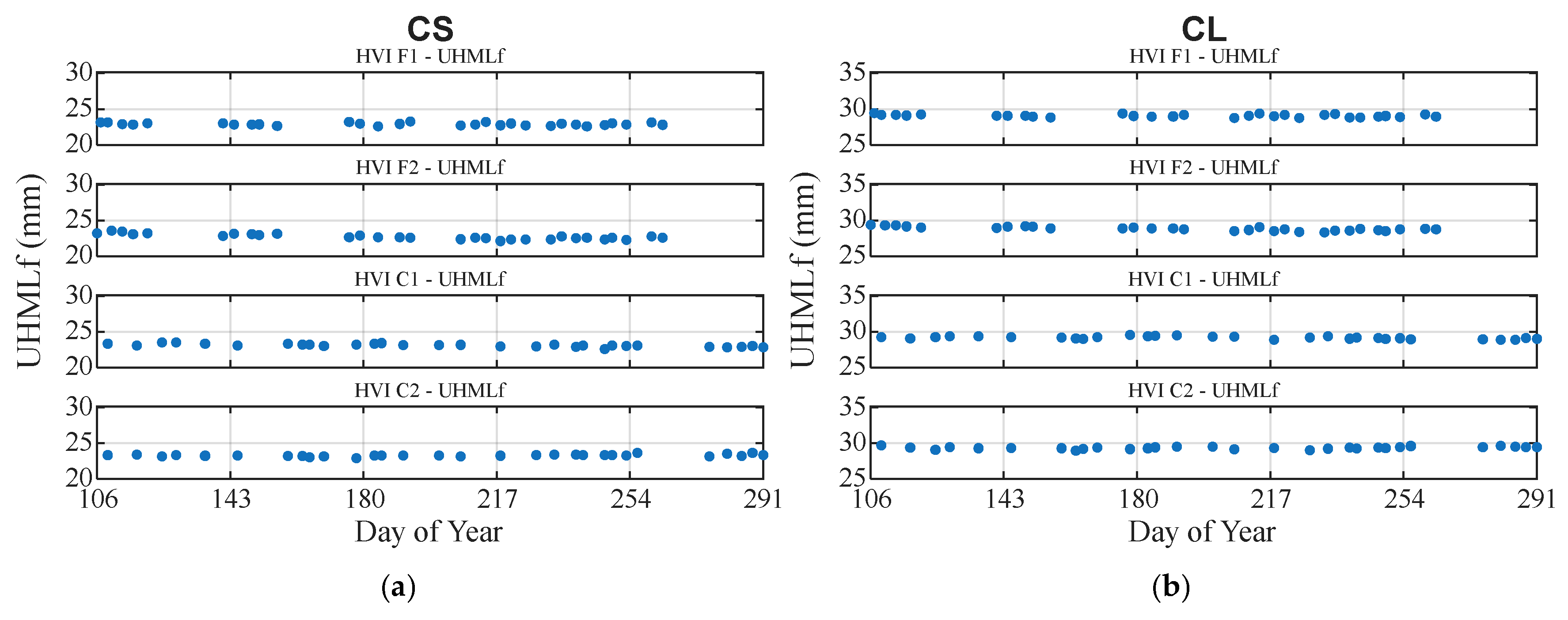
Starting with the measurements of the calibration samples, Figure 4 shows the average UHMLf measured in the four HVIs throughout the 30 days of testing. Visually, none of the HVIs show any trend in either the CL or CS samples.

Table 2. Statistical stability analysis for UHMLf of calibration samples. Note that the values are reported in units of 10⁻⁴.

HVI	Sample Type	Slope (mm/Day) (×10−4)	95% CI of Slope (mm/Day) (×10−4)	Remarks
F1	CL	−12	[−26, 2]	No significant trend
F2	CL	−45	[−58, −32]	Significant trend
C1	CL	−17	[−29, −5]	Significant trend
C2	CL	8	[−3, 20]	No significant trend
F1	CS	−9	[−22, 5]	No significant trend
F2	CS	−60	[−76, −44]	Significant trend
C1	CS	−28	[−38, −18]	Significant trend
C2	CS	11	[2, 21]	Significant trend

shows the results of these analyses for the calibration samples. In this table, the existing trend in the data is statistically significant when the upper and lower limits of the slope’s confidence interval do not include zero. There are some statistically significant trends, such as the UHMLf measurements of both CL and CS samples for HVI F2 and C1. For C2, a significant trend is observed only for CS samples, which is interesting because one might expect mechanical drift to affect both long and short fiber measurements. The important thing to note from Table 2 is that, even when there are statistically significant trends in the HVI measurements, the slope of the trend is around 10⁻³–10⁻⁴ mm/day. Given that HVI length measurements are typically rounded to the nearest hundredth of an inch in the US (0.01 inch or 0.254 mm), it could take weeks or months for the trend to begin to impact the least significant digit.

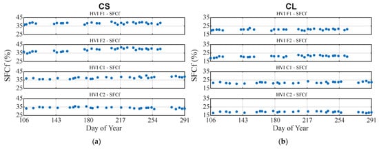
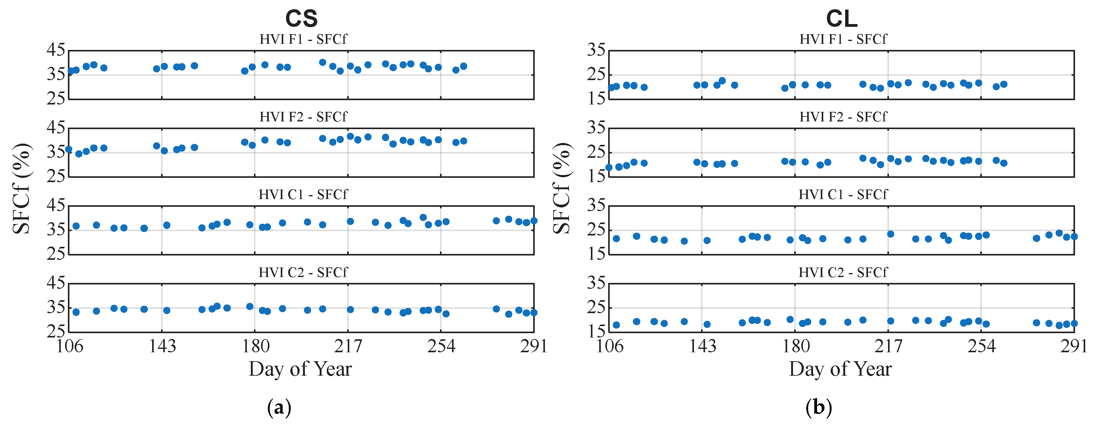
For SFCf, the results are similar; however, the visual stability analysis in Figure 5 shows that there is greater day-to-day variation in SFCf than in UHMLf. This is expected as short fiber content is generally more variable as a length parameter than others [28]. SFCf is calculated from the proportion of fibers below a specified length threshold and is therefore highly sensitive to small changes in the tail of the fiber length distribution. Minor measurement fluctuations near the short-fiber cutoff can result in relatively large changes in the calculated SFCf value. Parameters associated with the extremes of the fiber length distribution tend to exhibit higher uncertainty than mean-based length parameters. This increased variability can also affect calibration performance, as greater measurement uncertainty in the reference and test samples may reduce the precision of the resulting calibration equations and increase the residual error after calibration. Figure 5 demonstrates a small visible trend in F2 and C1.

Table 3. Statistical stability analysis for SFCf of calibration samples. Note that the values are reported in units of 10⁻³.

HVI	Sample Type	Slope (%/Day) (×10−3)	95% CI of Slope (%/Day) (×10−3)	Remarks
F1	CL	4	[−2, 9]	No significant trend
F2	CL	13	[7, 19]	Significant trend
C1	CL	8	[3, 13]	Significant trend
C2	CL	−2	[−7, 3]	No significant trend
F1	CS	4	[−3, 11]	No significant trend
F2	CS	31	[23, 40]	Significant trend
C1	CS	16	[10, 21]	Significant trend
C2	CS	−6	[−11, −2]	Significant trend

validates this visual assessment as it shows some statistically significant trends for these HVIs. It also shows a significant trend in C2 for the SFCf parameter of CS samples. This is similar to the UHMLf stability analysis, as it also showed significant trends in the case of only CS samples for C2. For both parameters, C2 appears to be more stable when measuring the length of longer cotton samples. On another note, although some HVIs show significant trends in their SFCf measurement, the slopes of these trends are small, around 10⁻²–10⁻³%/day. An equivalent parameter to SFCf is short fiber content (SFC), which is reported in AFIS. The AFIS reports SFC in the 10th of a percent (0.1%). As the slope of the trends of mechanical drift is smaller than the smallest percentage of SFC that AFIS reports, it would take days or weeks before there is any change in the SFC measurement caused by the drift.

We also performed this analysis on the other parameters (MLf, LHMLf) from the reconstructed length distribution. For these parameters, the analysis showed similar results compared to the above-mentioned two parameters, both visually and statistically. Similar to UHMLf and SFCf, we found no visible trend for the other parameters (shown in Figures S1 and S2). Statistically, there were significant trends present for HVI F2, C1, and C2 (shown in Tables S4 and S5). However, the slope of the trends was very small (around 10⁻²–10⁻³ mm/day). Since these other parameters are reported in 100ths of an inch, similar to UHMLf, it would take weeks or even months to change the reported output. We also analyzed the stability of the HVIs for 1.8% and 7.8% span length, which showed similar visual (Figures S3 and S4) and statistical results (Tables S6 and S7).

Overall, the statistical results reveal the presence of small but measurable trends, suggesting gradual mechanical drift in the instruments. However, in each case, the magnitude of the drift is sufficiently small that a prolonged period would be required before they produce a detectable change in the reported measurements.

3.1.2. USDA Evaluation Samples

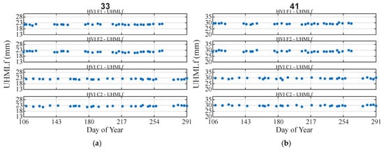
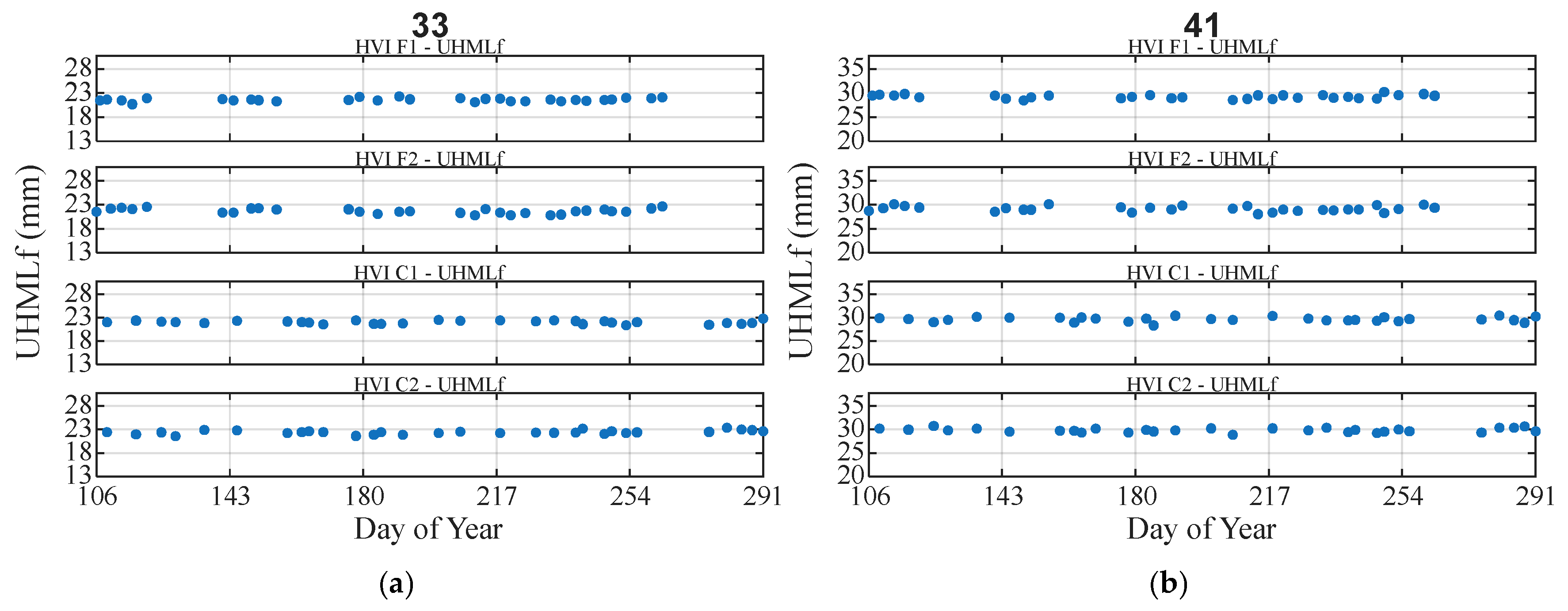
For the evaluation samples, Figure 6 shows a visual stability analysis for staple lengths 33 and 41. It can be observed for these samples that there is a higher variation between different days’ UHMLf measurements versus the calibration standards. Furthermore, all graphs in Figure 6 do not show any visible trend for the different staple lengths of USDA evaluation samples. The statistical stability analysis in

Table 4. Statistical stability analysis of UHMLf for USDA evaluation samples of staple lengths (a) 33 and (b) 41. Note that the values are reported in units of 10⁻⁴.

HVI	Staple Length	Slope (mm/Day) (×10−4)	95% CI of Slope (mm/Day) (×10−4)	Remarks
F1	33	14	[−11, 40]	No significant trend
F2	33	−30	[−68, 9]	No significant trend
C1	33	−7	[−30, 17]	No significant trend
C2	33	29	[3, 55]	Significant trend
F1	41	−1	[−32, 31]	No significant trend
F2	41	−17	[−59, 26]	No significant trend
C1	41	1	[−33, 35]	No significant trend
C2	41	−4	[−35, 28]	No significant trend

shows that only C2 for staple length 33 shows statistically significant trends. Even for this exception, the slope is very small (0.0029 mm/day) compared to the sample’s UHMLf values. Statistically, the analysis of the evaluation samples reveals fewer statistically significant trends than the calibration samples. Because there was greater day-to-day variation in these samples (due to testing only four repetitions versus 24 with the calibration samples), the confidence interval was wider, resulting in most trends being considered statistically insignificant.

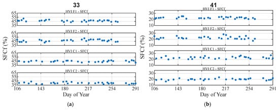
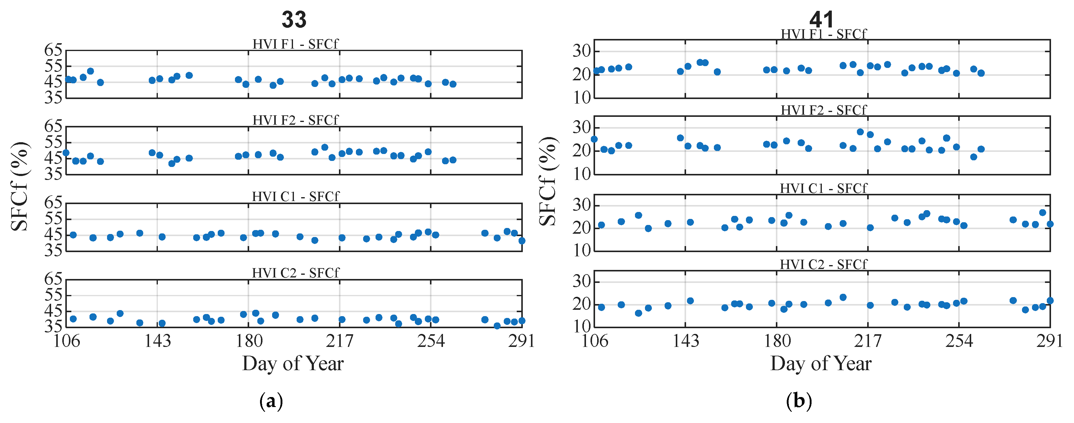
For SFCf, the analysis yields similar results to UHMLf. Visually, no trend is seen for any of the staple lengths tested in the HVIs (Figure 7). In the analysis in

Table 5. Statistical stability analysis of SFCf for USDA evaluation samples of staple lengths (a) 33 and (b) 41. Note that the values are reported in units of 10⁻³.

HVI	Staple Length	Slope (%/Day) (×10−3)	95% CI of Slope (%/Day) (×10−3)	Remarks
F1	33	−13	[−27, 1]	No significant trend
F2	33	15	[−4, 33]	No significant trend
C1	33	1	[−11, 12]	No significant trend
C2	33	−10	[−23, 2]	No significant trend
F1	41	−3	[−13, 7]	No significant trend
F2	41	−4	[−22, 13]	No significant trend
C1	41	7	[−6, 20]	No significant trend
C2	41	7	[−3, 16]	No significant trend

, none of the trends is statistically significant.

For the other parameters calculated from the reconstructed length distribution (MLf and LHMLf), no visible trends were seen (shown in Figures S5 and S6, respectively). In the statistical stability analysis, the evaluation sample yields results that differ slightly from those of the calibration samples. For these parameters, statistical analysis in Tables S8 and S9 shows that there are no statistically significant trends present. For the HVI-reported 1.8% and 7.8% SL, visually, the results were the same, with no identifiable trend (shown in Figures S7 and S8, respectively). However, a few significant trends were revealed in the statistical analysis, as shown in Tables S10 and S11. Nevertheless, similar to other parameters, the trends have very small slopes, which would take substantial time to have any impact on the measurements.

The absence of statistically significant trends for most USDA evaluation samples is likely attributable to their greater day-to-day variability. This increased variability may be explained by the fact that, unlike the calibration cottons, the evaluation cottons were not homogenized through blending prior to testing and therefore exhibited lower within-sample uniformity. Moreover, as previously mentioned, while the calibration bales were tested with 24 repetitions, the evaluation bales were tested with 4 repetitions. These two factors increased the range of 95% confidence intervals. Overall, the stability analysis of the calibration and evaluation samples shows that the HVIs used in this experiment have very little mechanical drift over time. This indicates that there is no need for frequent calibration on a single HVI when daily checks and proper maintenance are performed. However, the data showed that the HVIs behaved differently from one another, which might have led to differences in their measurements. This is explored in the next section.

3.2. Two-Point vs. Three-Point Calibration

During typical HVI calibration, a two-point linear regression is performed between the reference values and the averages of 12 repetitions of the long and short reference cottons. While two-point linear regression does not have any degrees of freedom, three-point linear regression provides us with a degree of freedom, which may lower variability and potentially improve calibration efficacy. Thus, we identified three bales to use for reference material: long, medium, and short.

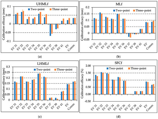
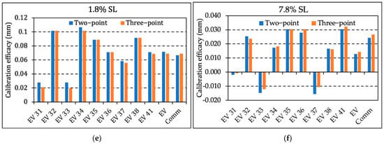
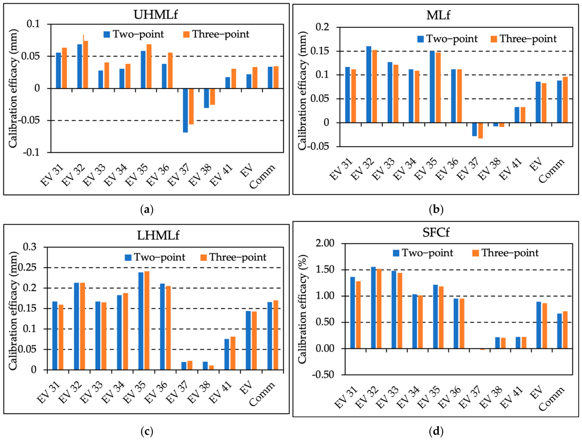
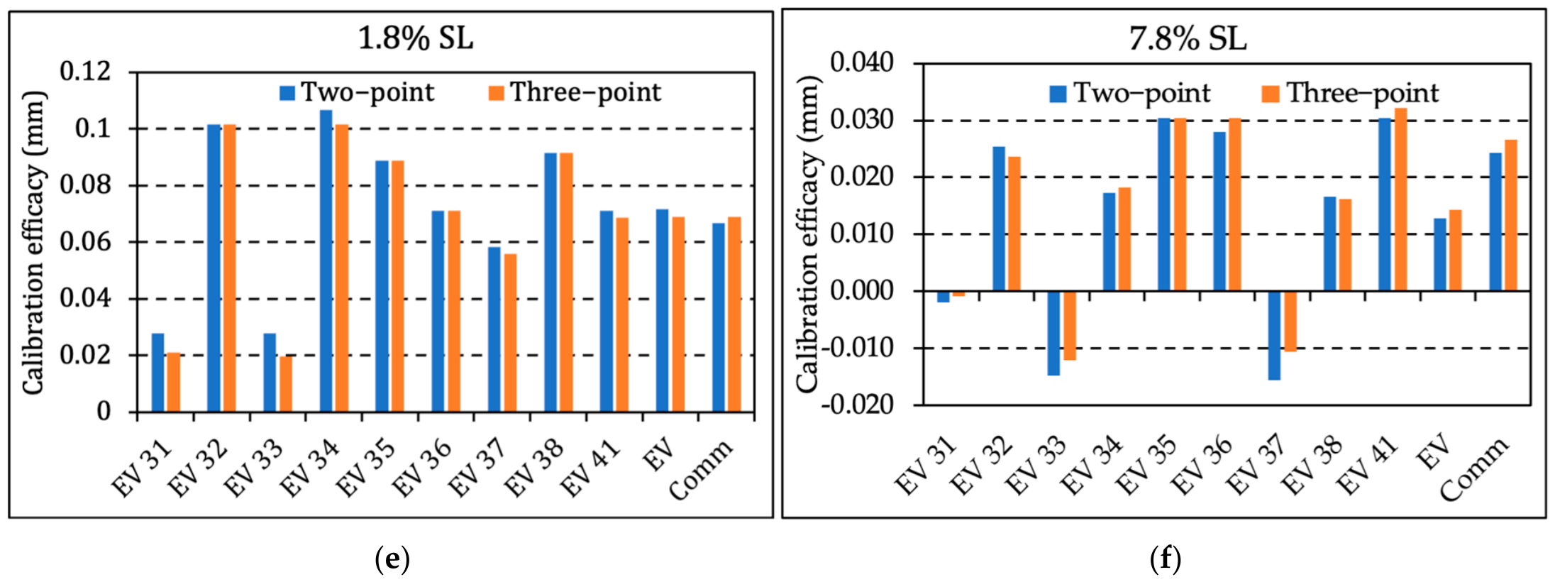
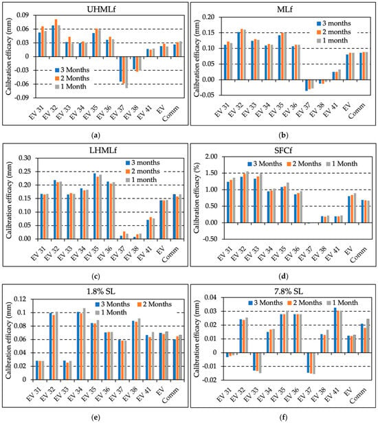
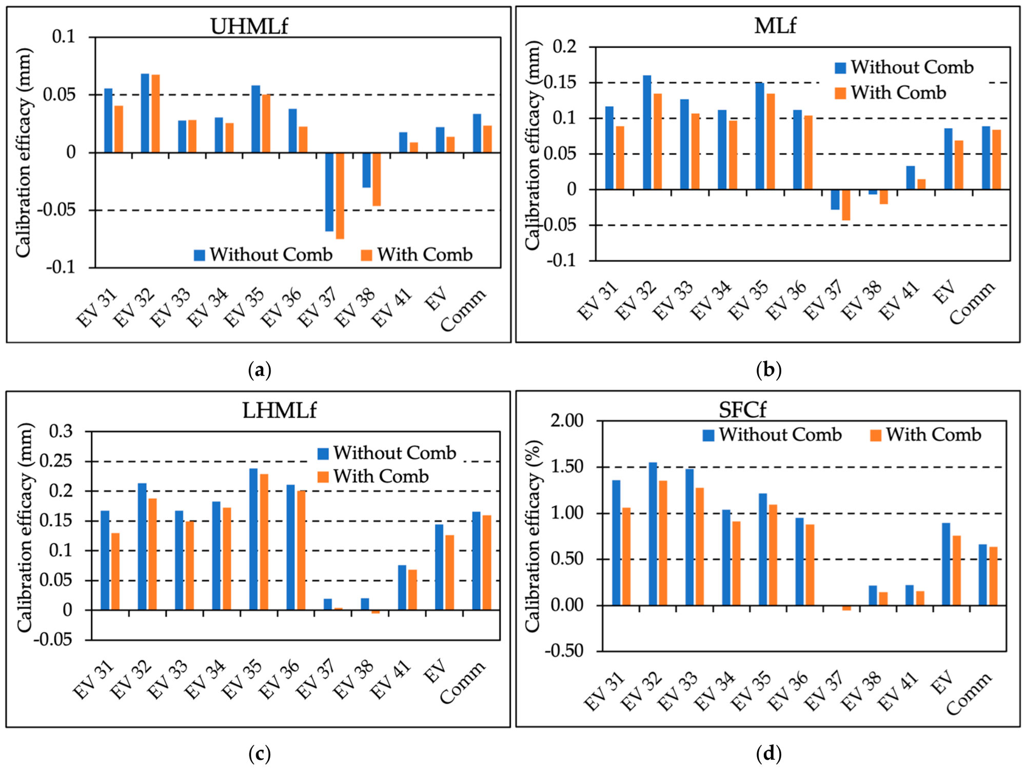
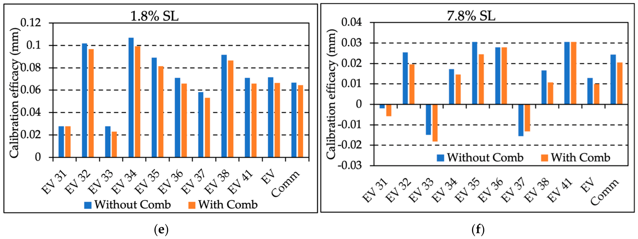
Figure 8 shows the comparison for each staple length of USDA evaluation samples tested in this study, as well as the average calibration efficacy for all evaluation and commercial samples, respectively shown as “EV” and “Comm”. For UHMLf and MLf (shown in Figure 8a,b), all EV staple lengths show positive calibration efficacy except EV 37 and 38. For example, in EV 32, the agreement among HVI measurements increased by an average of 0.09 mm. Regarding the difference in calibration efficacy between two-point and three-point calibration, the performance of both methods is quite similar. In some cases, the three-point calibration is slightly better; however, the differences are small (around 0.01–0.02 mm) compared to the total calibration efficacy. For SFCf (Figure 8d) and HVI-reported 1.8% and 7.8% span lengths (shown in Figure 8e and Figure 8f, respectively), the calibration efficacy is positive for most of the EV staple lengths and, on average, for both evaluation and commercial samples. The similar performance of the two calibration approaches is consistent with an approximately linear relationship between the reference and observed measurements over the range represented by the calibration standards. Under such conditions, the short- and long-staple calibration standards are sufficient to characterize the primary systematic differences among HVIs by defining the offset and slope of the calibration equation. Consequently, the inclusion of an additional medium-staple standard provides only limited new information, resulting in only marginal improvements in calibration efficacy.

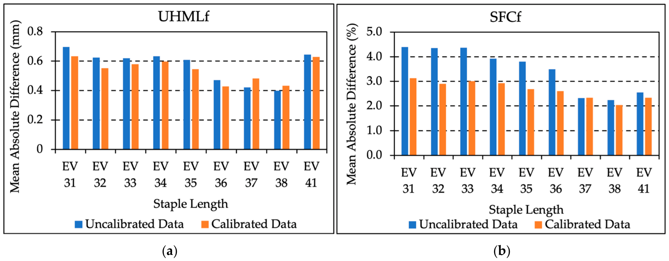
Since negative calibration efficacy was observed only for staple lengths 37 and 38, an analysis was conducted on the distribution of each staple length from 31 to 41. The pattern of distribution progression from one staple length to the next (i.e., 31 to 32) seemed consistent up to 37 and 38, which looked quite similar. Upon further analysis, Figure 9a,b showed that the mean absolute differences for staple lengths 37 and 38 are lower compared to all other staple lengths before calibration. Since the HVIs are already in good agreement for staple lengths 37 and 38, calibration does not yield further improvement in the agreement among HVIs.

Overall, the calibration method improves agreement or reduces differences among the HVIs for both HVI-reported length parameters and length parameters calculated from the reconstructed length distribution. Also, because this part of the study was iterated over 100 times, with each time choosing different days’ equations, the results demonstrate that the calibration method consistently yields positive outcomes and is not simply the result of a single favorable set of equations.

3.3. Varying the Calibration Frequency

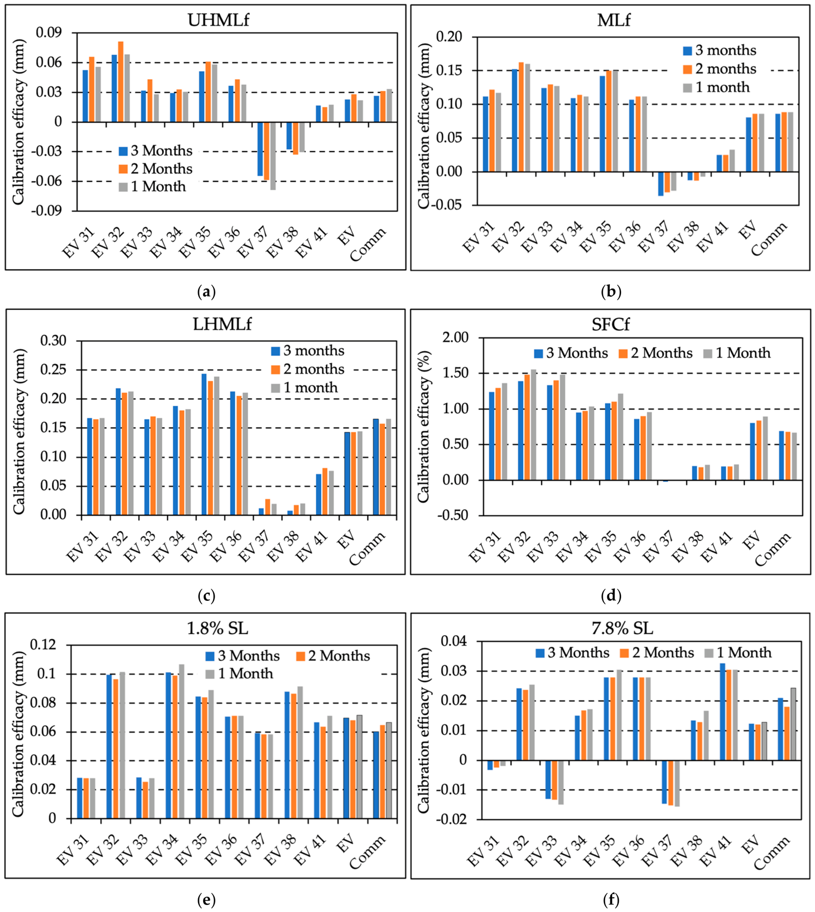
This analysis was conducted to evaluate whether calibrating more frequently improves the calibration efficacy. In Figure 10, the three bars above each EV staple length represent calibration efficacy during different intervals between calibrations. Two-point calibration is being used in this analysis since the previous section showed that both three-point and two-point calibration provide similar calibration efficacy. Figure 10a,b show that for UHMLf and MLf, respectively, there are very few differences between the calibration efficacies using different calibration frequencies. For example, in Figure 10b, for MLf on EV 32, calibrating every month improved agreement among HVIs by only about 0.01 mm compared to calibrating once every three months. Similar results can be seen for the other parameters, like LHMLf and SFCf (shown in Figure 10c and Figure 10d, respectively). For HVI-reported 1.8% and 7.8% span length (shown in Figure 10e,f), the calibration efficacy is almost identical for different intervals, although a slight average increase for more frequent calibrations is observed in some cases.

3.4. Applying Comb Checks

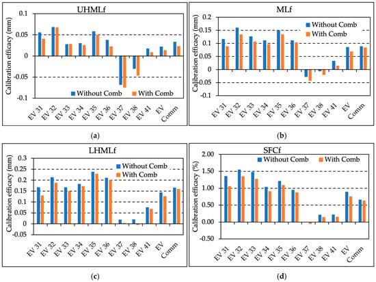
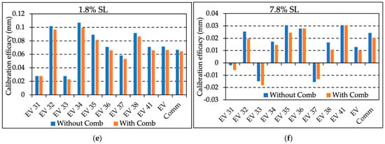
The central idea with comb checks is to remove outlying repetitions in order to reduce the variation within the observed reference samples, thereby reducing variation in the calibration equations. The goal of this analysis is to evaluate whether calibration works better if there is less variation within the repetitions measured. Figure 11 illustrates the comparison of calibration efficacies between using and not using comb checks. The orange bar represents how calibration efficacy changes when comb checks are used. Figure 11a–d show that calibration efficacy decreases slightly for parameters calculated from the reconstructed length distribution when comb checks are used. The change is very small compared to the overall calibration efficacy. For example, for the MLf measurement of EV 33, calibration efficacy decreases by about 0.02 mm when comb checks are used. For HVI-reported parameters like 1.8% and 7.8% span length, there is almost no change or very little change when using calibration with comb checks (shown in Figure 11e,f).

A plausible explanation for the lack of improvement in calibration efficacy following the application of comb checks is the experimental design employed in this study. As discussed previously, the primary purpose of comb checks is to identify and exclude outlying measurements, thereby reducing measurement variability and improving calibration stability. However, the calibration procedure evaluated in this study was based on 24 replicate measurements, compared with the 12 replicates used in the current HVI calibration protocol. The increased number of replicates inherently reduces the influence of random measurement variation through averaging, thereby improving measurement precision even in the absence of comb checks. Consequently, the additional benefit of removing a limited number of outlying observations may have been relatively small, resulting in minimal differences in calibration efficacy between procedures with and without comb checks. We hypothesize that this alone limits the usefulness of comb checks. It is also possible that a different method of choosing tolerance values (rather than using the standard deviation) could be more useful. These ideas could be explored in further research.

4. Conclusions

In this paper, we discussed the development of a calibration method for the new fiber length parameters calculated from the reconstructed length distribution obtained from Turner’s algorithm. The calibration method was inspired by the calibration strategy of Tesema’s prior work on correction equations. Since HVI provides faster testing times than AFIS, calibrating the new parameters from the reconstructed length distribution would enable more rapid acquisition of detailed information about the cotton fiber sample. At the beginning of this study, we performed a stability analysis on the uncalibrated measurements. This analysis showed some statistically significant trends; however, the slopes were so small that it would take a substantial amount of time to produce any change in the reported measurement values. This suggests that frequent calibration is unlikely to yield meaningful improvements under operating conditions in which the lab environment and the HVIs are well-maintained. If daily checks and regular maintenance are performed, an HVI should provide stable measurements for weeks or more. However, the mechanical drift would eventually require a correction.

The calibration efficacy analysis showed an overall improvement in agreement among the HVIs across different sets of samples, indicating that the calibration method is effective. As for the difference between two- and three-point calibration, both provided about the same efficacy. While in some cases the addition of the medium-length sample may have improved the efficacy slightly, 50% more effort and material are needed to perform calibration with a third bale. We believe that the minor improvement in calibration is not worth the added time and expense. Regarding calibration frequency, calibrating more frequently did not significantly improve agreement among HVIs. This result relates back to our stability analysis, which showed very little to no drift within the HVIs during the six-month study period. For the comb checks, the results show that the calibration efficacy stayed almost the same. As 24 repetitions were used for the calibration samples, this result makes sense, as a larger number of combs reduces variability in the mean.

Overall, the calibration method discussed in this study may provide breeders with access to more detailed, calibrated length measurements on the HVI. These calibration procedures may facilitate future adoption of fibrogram-derived length parameters in breeding and commercial testing applications.

References

- Faulkner, W.B.; Hequet, E.F.; Wanjura, J.; Boman, R. Relationships of cotton fiber properties to ring-spun yarn quality on selected High Plains cottons. Text. Res. J. 2012, 82, 400–414. [Google Scholar] [CrossRef] [Scilit]
- Günaydin, G.K.; Soydan, S.S.; Palamutçu, S. Evaluation of cotton fibre properties in compact yarn spinning processes and investigation of fibre and yarn properties. Fibres Text. East. Eur. 2018, 26, 23–34. [Google Scholar] [CrossRef] [Scilit]
- Brown, H.B. Cotton: History Species, Varieties, Morphology, Breeding, Culture, Diseases, Marketing, and Uses; McGraw-Hill: Columbus, OH, USA, 1938. [Google Scholar]
- May, O.L.; Jividen, G.M. Genetic modification of cotton fiber properties as measured by single-and high-volume instruments. Crop Sci. 1999, 39, 328–333. [Google Scholar] [CrossRef] [Scilit]
- Perkins, H.H., Jr.; Ethridge, D.E.; Bragg, C.K. Fiber. Cotton 1984, 24, 437–509. [Google Scholar] [CrossRef] [Scilit]
- Parsi, R.D.; Kakde, M.V.; Pawar, K.; Patil, R.P. Influence of fibre length on ring spun yarn quality. Int. J. Res. Sci. Innov. 2016, 3, 154–156. [Google Scholar] [CrossRef] [Scilit]
- Abdkader, A.; Hossain, M. A critical review on recent developments and solutions in the high-speed ring spinning process. Text. Res. J. 2023, 93, 5485–5504. [Google Scholar] [CrossRef] [Scilit]
- Bauer, P.J.; Foulk, J.S.; Gamble, G.R.; Sadler, E.J. A comparison of two cotton cultivars differing in maturity for within-canopy fiber property variation. Crop Sci. 2009, 49, 651–657. [Google Scholar] [CrossRef] [Scilit]
- Feng, L.; Bufon, V.B.; Mills, C.I.; Hequet, E.; Bordovsky, J.P.; Keeling, W.; Boman, R.; Bednarz, C.W. Effects of irrigation, cultivar, and plant density on cotton within-boll fiber quality. Agron. J. 2011, 103, 297–303. [Google Scholar] [CrossRef] [Scilit]
- Kelly, B.; Abidi, N.; Ethridge, D.; Hequet, E.F. Fiber to fabric. Cotton 2015, 57, 665–744. [Google Scholar] [CrossRef] [Scilit]
- Kelly, C.M.; Hequet, E.F.; Dever, J.K. Breeding for improved yarn quality: Modifying fiber length distribution. Ind. Crops Prod. 2013, 42, 386–396. [Google Scholar] [CrossRef] [Scilit]
- Kim, H.J.; Thyssen, G.N.; Delhom, C.D.; Fang, D.D.; Naoumkina, M.; Florane, C.B.; Li, P.; Jenkins, J.N.; McCarty, J.C.; Zeng, L. Genome-wide association studies of bundle and single fiber length traits reveal the genetic basis of within-sample variation in upland cotton fiber length. Front. Plant Sci. 2024, 15, 1472675. [Google Scholar] [CrossRef] [Scilit] [PubMed]
- Delhom, C.D.; Hequet, E.F.; Kelly, B.; Abidi, N.; Martin, V.B. Calibration of HVI cotton elongation measurements. J. Cotton Res. 2020, 3, 31. [Google Scholar] [CrossRef] [Scilit]
- Sayeed, M.S.; Schumann, M.; Wanjura, J.; Kelly, B.R.; Smith, W.; Hequet, E.F. Characterizing the total within-sample variation in cotton fiber length using the High Volume Instrument fibrogram. Text. Res. J. 2021, 91, 175–187. [Google Scholar] [CrossRef] [Scilit]
- Krowicki, R.; Ramey, H., Jr. An Examination of the Digital Fibrograph Length Uniformity Index 1. Crop Sci. 1984, 24, 378–381. [Google Scholar] [CrossRef] [Scilit]
- Bragg, C.K.; Shofner, F.M. A rapid, direct measurement of short fiber content. Text. Res. J. 1993, 63, 171–176. [Google Scholar] [CrossRef] [Scilit]
- Liu, Y.; Chang, S. Comprehensive analysis of cotton fiber infrared maturity distribution and its relation to fiber HVI and AFIS properties. Fibers Polym. 2024, 25, 1127–1136. [Google Scholar] [CrossRef] [Scilit]
- Altintas, P.; Simonton, J.; Beruvides, M. TexTile Technology: Pilot Study to Examine the Relationship between AFIS Fiber Properties and White Speck Occurrence. J. Cotton Sci. 2007, 11, 159–167. [Google Scholar]
- Gardunia, B.W.; Braden, C.; Hequet, E.; Smith, C.W. Applying quantile regression to analysis of AFIS cotton fiber distribution. Crop Sci. 2008, 48, 1328–1336. [Google Scholar] [CrossRef] [Scilit]
- Wang, H.; Sari-Sarraf, H.; Hequet, E. A Reference Method for Automatic and Accurate Measurement of Cotton Fiber Length. In Proceedings of the 2007 Beltwide Cotton Conference, New Orleans, LA, USA, 9–12 January 2007. [Google Scholar]
- Liu, Y. Variability of Fiber AFIS Length and Maturity within and Among Upland Cotton Cultivars. J. Nat. Fibers 2024, 21, 2356694. [Google Scholar] [CrossRef] [Scilit]
- Gautam, S. Evaluation of OFDA 4000 for Cotton Fiber Ribbon-Width and Length Measurement. Master’s Thesis, Texas Tech University, Lubbock, TX, USA, 2024. [Google Scholar]
- Turner, C.; Sayeed, M.S.; Hequet, E. Reconstruction of the cotton fiber length distribution from a High Volume Instrument® fibrogram. Text. Res. J. 2023, 93, 1651–1669. [Google Scholar] [CrossRef] [Scilit]
- Tesema, S.F.; Sayeed, M.S.; Turner, C.; Kelly, B.R.; Hequet, E.F. An approach for obtaining stable, reproducible, and accurate fibrogram measurements from High Volume Instruments. Agronomy 2022, 12, 1120. [Google Scholar] [CrossRef] [Scilit]
- Chu, Y.-T.; Riley, C.R., Jr. New interpretation of the fibrogram. Text. Res. J. 1997, 67, 897–901. [Google Scholar] [CrossRef] [Scilit]
- Podder, I.; Fischl, T.; Bub, U. Smart calibration and monitoring: Leveraging artificial intelligence to improve MEMS-based inertial sensor calibration. Complex Intell. Syst. 2024, 10, 7451–7474. [Google Scholar] [CrossRef] [Scilit]
- Sayeed, M.S.; Kelly, B.R.; Turner, C.; Hequet, E.F. Investigation of a multivariate correction method for HVI fibrogram measurements. Agronomy 2022, 12, 460. [Google Scholar] [CrossRef] [Scilit]
- Thibodeaux, D.; Senter, H.; Knowlton, J.; McAlister, D.; Cui, X. Measuring the short fiber content of cotton. Cotton: Nature’s high-tech fiber. In Proceedings of the World Cotton Research Conference-4, Lubbock, TX, USA, 10–14 September 2007. [Google Scholar]
Disclaimer/Publisher’s Note: The statements, opinions and data contained in all publications are solely those of the individual author(s) and contributor(s) and not of MDPI and/or the editor(s). MDPI and/or the editor(s) disclaim responsibility for any injury to people or property resulting from any ideas, methods, instructions or products referred to in the content. |
© 2026 by the authors. Licensee MDPI, Basel, Switzerland. This article is an open access article distributed under the terms and conditions of the Creative Commons Attribution (CC BY) license.