1. Introduction
The use of GFRP bars as reinforcement in concrete structures has gained attention as a viable alternative to conventional steel reinforcement, particularly for applications requiring high durability. However, GFRP in structural applications is limited by its brittle behavior and lack of ductility when compared to steel. Unlike steel, GFRP does not exhibit yielding behavior, which leads to the need for hybrid GFRP–steel RC systems to leverage the ductility of steel and the tensile strength of GFRP. As a result, such composite nature of the reinforcement system requires further optimization, making the understanding of its bond interaction with concrete critical for safe and effective structural performance. The bond mechanism governs load transfer between the reinforcement and surrounding concrete and directly influences stiffness, cracking behavior, and failure mode. Previous studies [
1,
2] have shown that the bond characteristics and behavior of GFRP RC structures differ significantly from those of steel bars, primarily due to differences in mechanical properties and surface morphology. Recent experimental studies on steel–CFRP interfaces in low-strength concrete have further underscored the critical role of bond–slip behavior in governing the overall structural response [
3]. These differences underscore the need for a detailed understanding of the bond mechanics unique to GFRP-reinforced concrete systems.
Existing bond models based on predefined functional forms (e.g., linear, exponential, and polynomial) often fail to capture the complex, nonlinear, and multi-parameter nature of GFRP–concrete bond behavior under pull-out force. These models rely on trial-and-error assumptions about physical relationships, which may not reflect the true mechanics of bond interactions. They also struggle to account for the combined effects of variables such as concrete strength, bar surface, diameter, and environmental factors. As a result, their generalizability is limited, especially when compared to machine learning approaches that can model complex, implicit relationships.
To address these limitations, this study introduces an FE modeling approach that incorporates an ANN trained on experimental data to predict the full bond–slip relationship. Unlike conventional models that rely on predefined functional forms, the ANN captures complex, nonlinear interactions among key bond-influencing parameters. These parameters often exhibit coupled effects that are difficult to model analytically. By embedding the ANN directly into the FE analysis, the model can simulate the complete evolution of bond stress and slip, rather than relying on simplified assumptions or peak values. This enables a more realistic representation of the bond interface and the resulting load transfer mechanisms. The ANN’s ability to learn from empirical data and generalize across varying conditions allows the FE model to adapt to a broader range of material configurations and loading scenarios, improving accuracy and reducing reliance on empirical calibration. As such, the ANN-integrated FE framework presents a more robust and versatile modeling strategy for hybrid GFRP–steel reinforced concrete systems.
It should be noted that this study focuses on establishing the ANN–FE integration framework using baseline monotonic pull-out data at ambient temperature. While durability is a critical advantage of GFRP, the modeling of long-term environmental degradation requires this baseline framework to be established first.
2. Theoretical Background
2.1. Existing Bond Models
Bond models for GFRP-reinforced concrete are typically developed from experimental observations and are widely used for design and analysis. Most existing models fall into two categories: simplified empirical equations and constitutive bond stress–slip relationships.
Empirical models, such as those found in ACI 440.1R and fib Bulletin 14 [
4,
5], predict maximum bond strength as a function of concrete compressive strength, bar diameter, and embedment length. These models are straightforward and easily integrated into design procedures but are limited in scope. Developed through regression analysis of specific test setups, they often fail to capture the influence of surface treatments, environmental exposure, and material variability [
6,
7,
8,
9]. Additionally, they reduce the bond behavior to a peak value, offering little insight into the full stress–slip response or post-peak degradation.
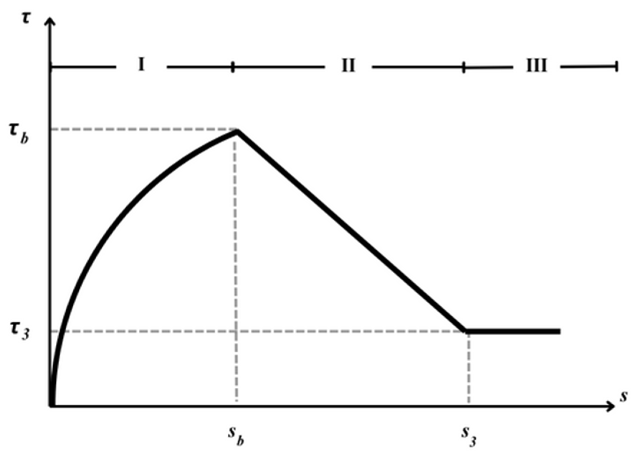
More advanced models aim to describe the entire bond stress–slip relationship using idealized constitutive formulations. A widely cited example is the modified Bertero–Eligehausen–Popov (mBPE) model [
10], which represents bond behavior in three stages as shown in
Figure 1. In this diagram, the vertical axis
τ represents the bond stress (MPa), and the horizontal axis
s represents the relative slip (mm). Key parameters include the peak bond stress (
τu) at slip (s
b) and the residual friction stress (
τ3) at slip (
s3). Additionally, the segments in the illustration represent (I) nonlinear elastic response due to chemical adhesion and bearing, (II) softening from crack development and debonding, and (III) residual stress governed by friction. Although more descriptive, these models still rely on simplifications and require case-specific calibration of parameters such as peak bond stress, slip, and softening exponents [
11,
12,
13,
14].
2.2. Need for Integrating FE Analysis with ANN Modeling
Machine learning (ML) techniques have recently emerged [
15] as powerful tools for predicting bond behavior in GFRP–RC systems. The bond response is inherently dependent on multiple interacting parameters, including bar surface texture, concrete strength, embedment depth, and environmental exposure, making it well-suited for ML approaches [
16,
17,
18]. For instance, recent works have successfully utilized ML-driven reliability analysis for bond prediction [
19] and XML-based modeling for shear capacity evaluation [
20], demonstrating the growing efficacy of advanced computational tools in FRP–RC analysis. Similarly, studies applying Support Vector Regression (SVR), Random Forests, and ANNs have reported substantial improvements in prediction accuracy compared to the bond models developed using other methods [
21,
22].
Among the ANN techniques, the feedforward backpropagation ANNs have shown particular promise for modeling GFRP–concrete bond behavior [
23]. These models excel at pattern recognition, enabling accurate prediction of bond strength and behavior across a range of shear forces on the rebar, even with limited datasets. Notably, they have achieved mean squared error reductions of up to 40% compared to other ML algorithms [
24]. While the interpretability of ANNs is often critiqued, recent advances in weight visualization and sensitivity analysis allow greater insight into variable importance, improving their applicability in engineering contexts [
25,
26,
27].
Despite their predictive power, standalone ANN models are limited by their abstraction from physical principles. They do not inherently model stress distribution, strain compatibility, or failure mechanisms at the bond interface, which are phenomena that are central to accurate structural simulation [
21,
28,
29]. FE analysis, by contrast, is grounded in continuum mechanics and provides detailed insights into local stress fields, crack initiation, and progressive failure. However, traditional FE models often struggle to represent the stress–slip story of the GFRP–concrete contact, especially under cyclic loading or environmental exposure.
An approach that integrates ANN predictions into FE analysis offers a solution that could lead to more accurate simulations. By using ANN-derived bond–slip curves as input to FE to define the interface elements, the model benefits from the adaptability of ANNs and the more accurate predictions from FE simulation [
30,
31]. This integrated framework enables accurate simulation of bond degradation and failure progression, offering new insights for the design and reliability assessment of GFRP–RC systems.
While previous studies have often limited ANN applications to predicting peak bond strength, recent work by Allouzi et al. [
32] emphasizes the value of modeling the entire bond–slip response. However, a critical research gap remains: the full integration of ANN-predicted bond–slip relationships into FE platforms.
3. Experimental Database
The pull-out experimental data used in this work was gathered from a previous study according to the experimental procedure described in [
33,
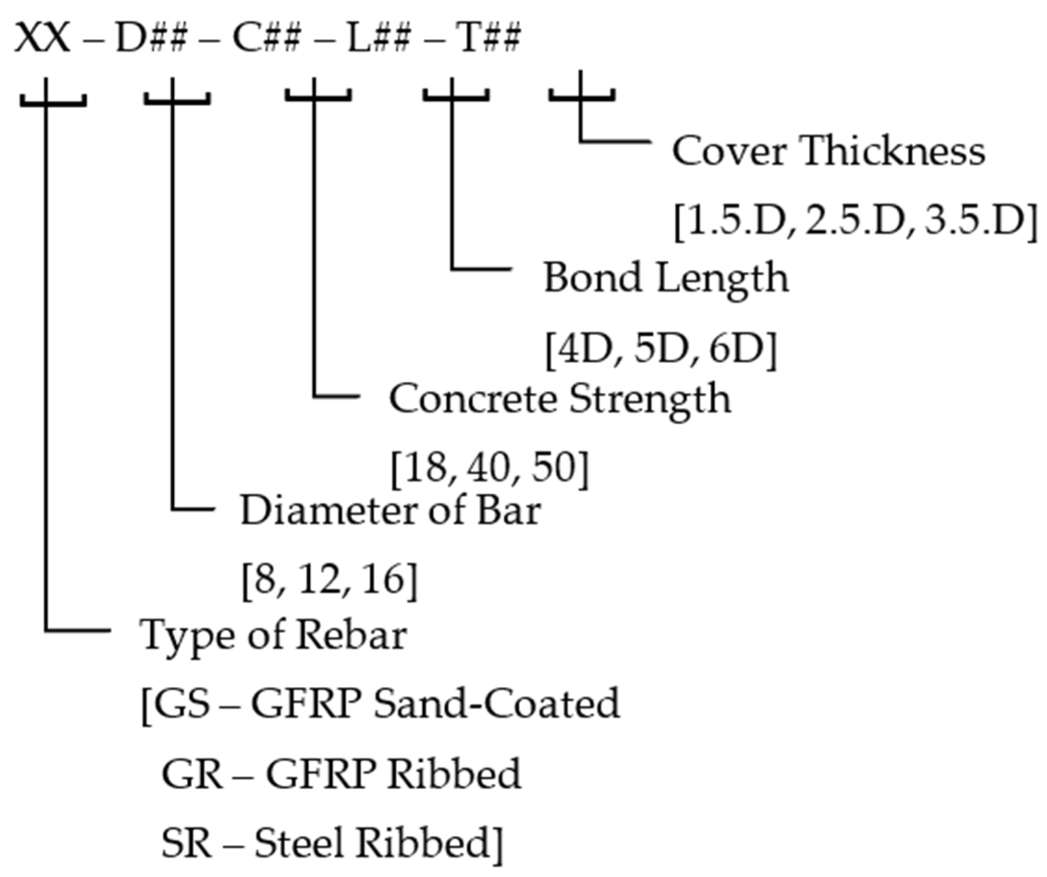
34]. The description of the sample designation and configuration is illustrated in
Figure 2.
This study investigated the bond behavior of GFRP rebars with sand-coated and ribbed surfaces in concrete with varying concrete strengths and various diameters. The experimental data was derived from an investigation [
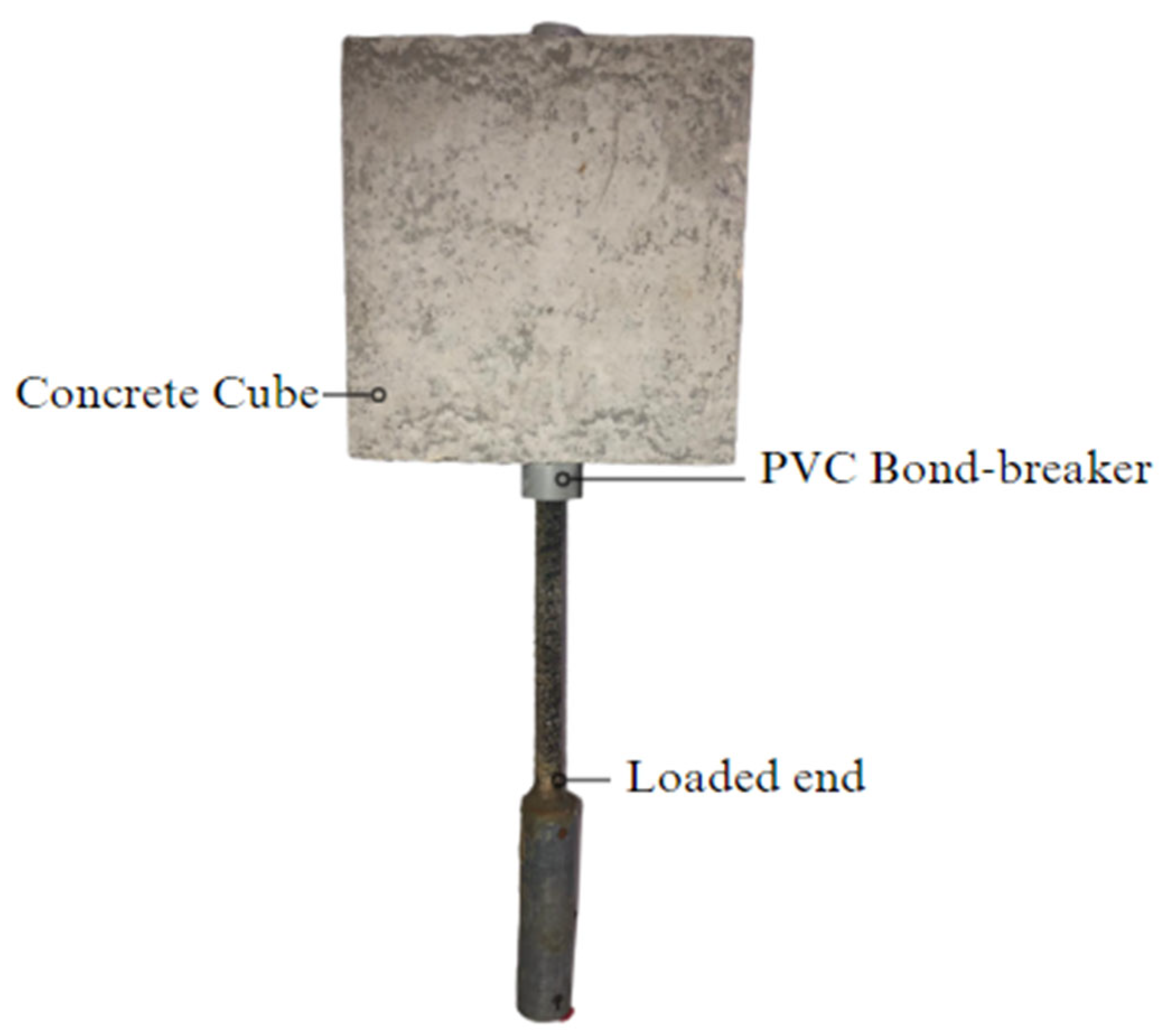
33] into two surface morphologies: sand-coated and ribbed. The rebars were sourced from local industry suppliers as ‘off-the-shelf’ materials and used as supplied in their original form. Both types were produced using E-glass fibres embedded in a vinyl ester resin matrix via the pultrusion process. The sand-coated bars incorporated a silica-sand layer bonded to the outer resin, while the ribbed bars featured helical protrusions formed during pultrusion. Following ACI 440 3R-14, GFRP bars were embedded in 150 × 150 × 150 mm concrete blocks, as shown in
Figure 3, and all specimens were cured for at least 28 days before pull-out testing. The variation in concrete compressive strength was achieved by adjusting the water-to-cement (
w/
c) ratio and the proportions of fine and coarse aggregates in the mix design. No admixtures were used for the lower-strength batches. In the configuration of the pull-out specimen shown in
Figure 3, the ‘Loaded end’ denotes the section of the rebar subjected to the tensile pull-out force. A ‘PVC Bond-breaker’ sleeve is installed at the interface to prevent local concrete crushing and to accurately delimit the effective bonded length within the ‘Concrete Cube’.
The pull-out tests were conducted using a calibrated Universal Testing Machine (UTM). The concrete specimen was seated against a rigid steel reaction frame which restrained the top face of the concrete block, allowing the GFRP bar to pass through the center for gripping. To ensure a quasi-static response, the load was applied under displacement control at a constant rate of 1.0 mm/min until bond failure occurred. The applied load and relative slip between the bar and concrete were recorded continuously throughout the test. A study [
33] has captured bond–slip behavior, as the relative slip between the GFRP bar and the concrete was monitored using two Linear Variable Differential Transformers (LVDTs). One LVDT was positioned at the loaded end to measure total displacement, while a second LVDT recorded slip at the free end. The actual bond slip was calculated by subtracting the elastic deformation of the bar from the loaded-end displacement.
This parametric investigation aimed to explore the influence of rebar surface texture, diameter, and concrete strength on bond behavior. The parameters and variables included in this study are detailed in
Table 1. The values for embedment length and cover thickness were determined as specific multiples of the bar diameter (
db) to normalize the geometric conditions across different bar sizes.
The experimental results indicate that bond strength between GFRP bars and concrete is primarily influenced by bond length, bar diameter, and concrete strength, whereas cover thickness exhibited a comparatively minor effect. Shorter bond lengths (48 mm) and smaller bar diameters (8 mm) yielded the highest bond strengths, measuring 18.3 MPa and 14.8 MPa, respectively. In contrast, increasing bond length and bar diameter led to a notable reduction in bond performance. Concrete strength demonstrated a nonlinear influence: bond strength increased from 7.1 MPa at 32 MPa concrete to 10.5 MPa at 40 MPa, with marginal gains observed at 50 MPa (11.5 MPa). Similarly, cover thickness showed a slight nonlinear trend, with bond strength peaking at 12.2 MPa for 30 mm cover, followed by a slight decline to 11.5 MPa at 42 mm.
4. ANN Modeling for Bond Behavior
The development of the ANN model used to predict the bond–slip behavior between GFRP bars and concrete is outlined as follows. The model was designed to capture the nonlinear and multi-parametric nature of bond interaction and to generate continuous bond–slip curves that could be directly integrated into finite element simulations.
4.1. Architecture and Learning Framework
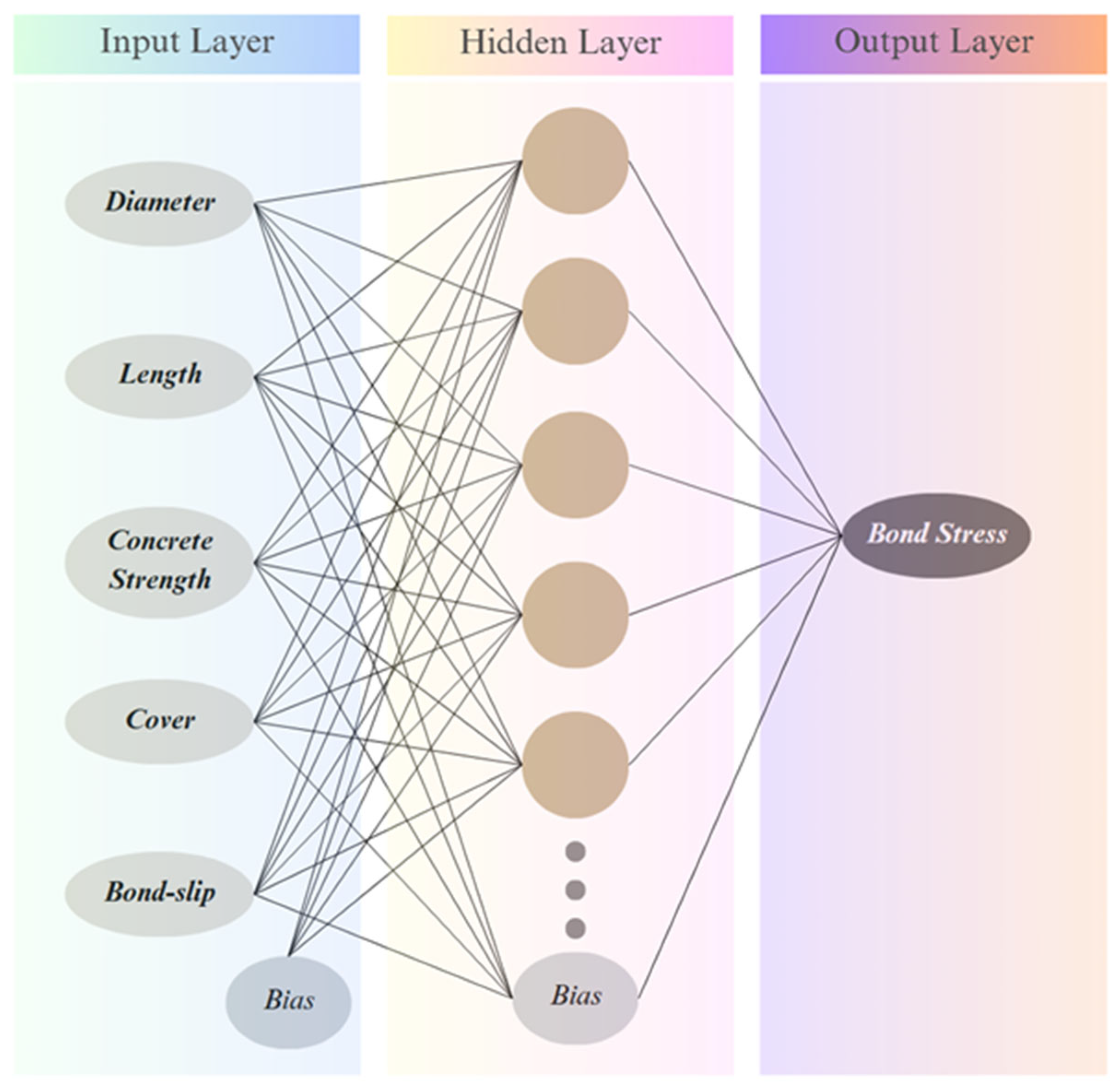
A feedforward backpropagation ANN was developed with hidden layers consisting of 12 neurons. The architecture, shown in
Figure 4, adopts 5-n-1 where the five input features represent the following: bar diameter (mm), embedment length (mm), concrete compressive strength (MPa), cover thickness (mm), and slip value (mm).
The output of the network is the corresponding bond stress (MPa). A logistic sigmoid activation function was used in the hidden layer to capture nonlinear interactions, and a linear activation function was applied at the output node to allow continuous prediction of bond stress. A single-layer architecture with 10 neurons offered optimal performance with fewer risks of overfitting, while retaining good generalization. This architecture also allows for easier integration with FE modeling routines.
The dataset was derived from over 1000 experimental data points obtained through laboratory pull-out tests under varying conditions. Prior to training, the MATLAB R2020b Neural Network Toolbox automatically applied its default pre-processing function (mapminmax) to the input and target data. This procedure scales each variable to a normalized range (default [−1, 1] [−1, 1] [−1, 1]) to improve numerical stability and convergence. The scaling is internally reversed after training to return predictions in the original physical units (MPa for bond stress).
The dataset was randomly divided into three subsets: training (70%), validation (15%), and testing (15%). This partitioning ensured balanced coverage of the input space and allowed robust evaluation of the model’s generalization capability. Data shuffling was performed prior to splitting to eliminate ordering biases.
It is noted that the ANN is a data-driven model trained on a specific dataset. Consequently, the model’s validity is currently established for monotonic loading within the experimental ranges defined in
Table 1 (GFRP diameters ≤ 16 mm and concrete strength ≤ 50 MPa). Application of the model outside these boundaries (extrapolation) requires further verification.
4.2. Training Methodology
The Levenberg–Marquardt optimization algorithm was employed to train the ANN, given its effectiveness in handling nonlinear regression problems and rapid convergence. Weights and biases were initialized randomly, and training was conducted over 100 epochs with early stopping enabled.
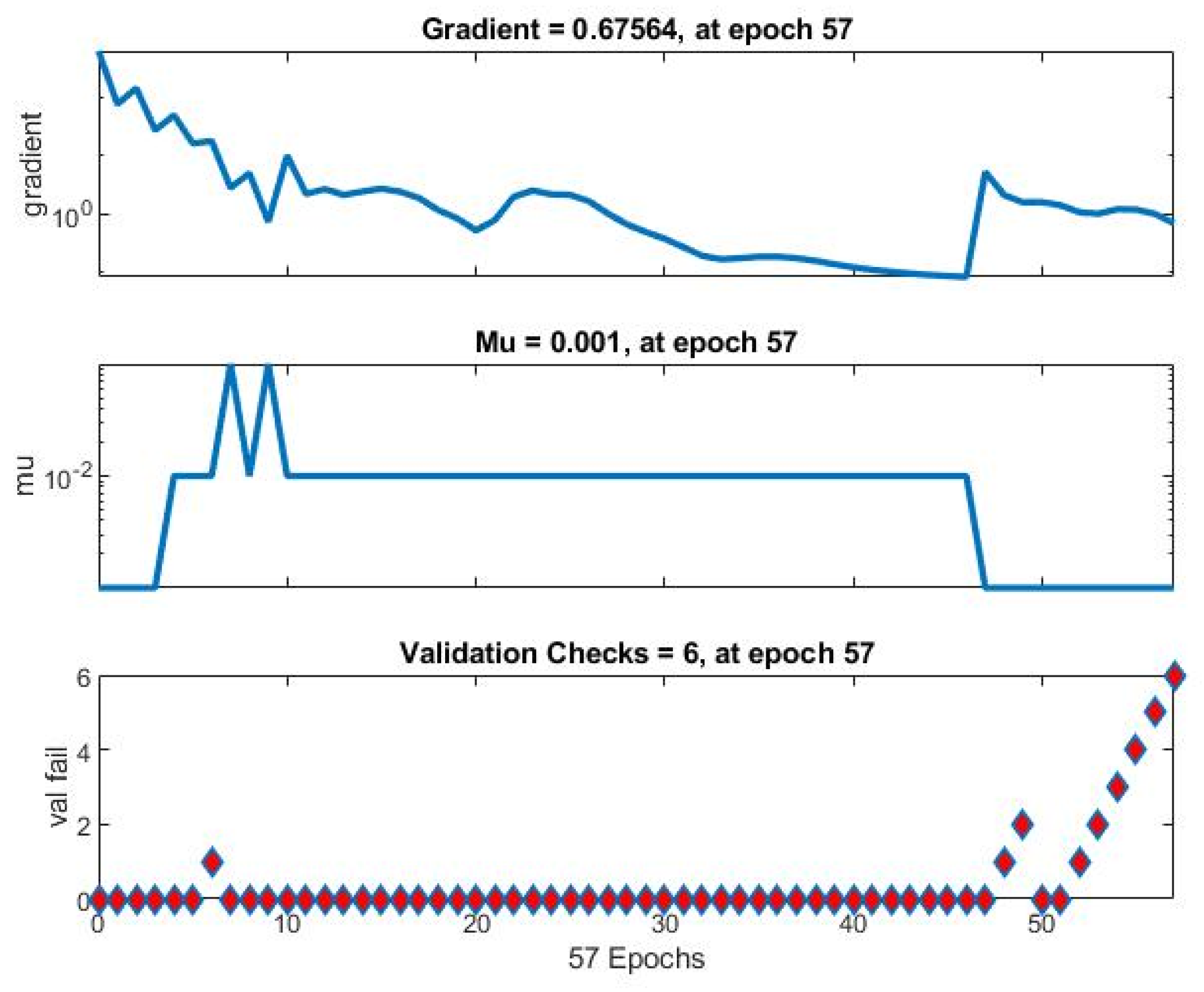
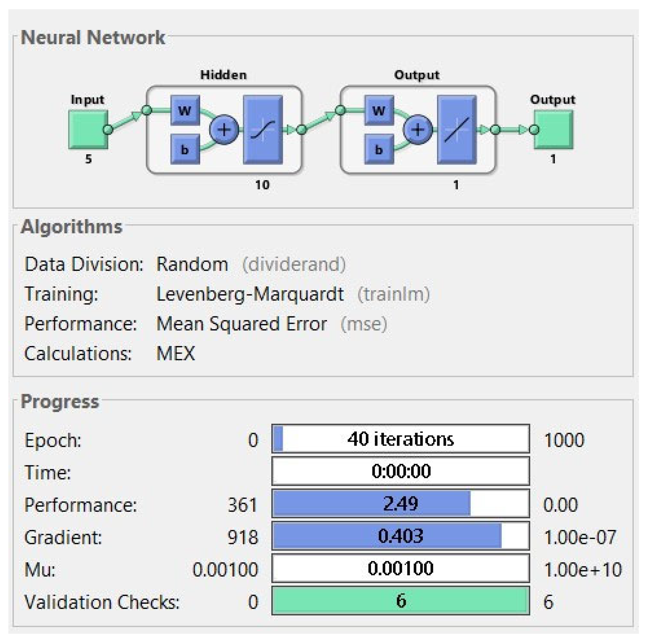
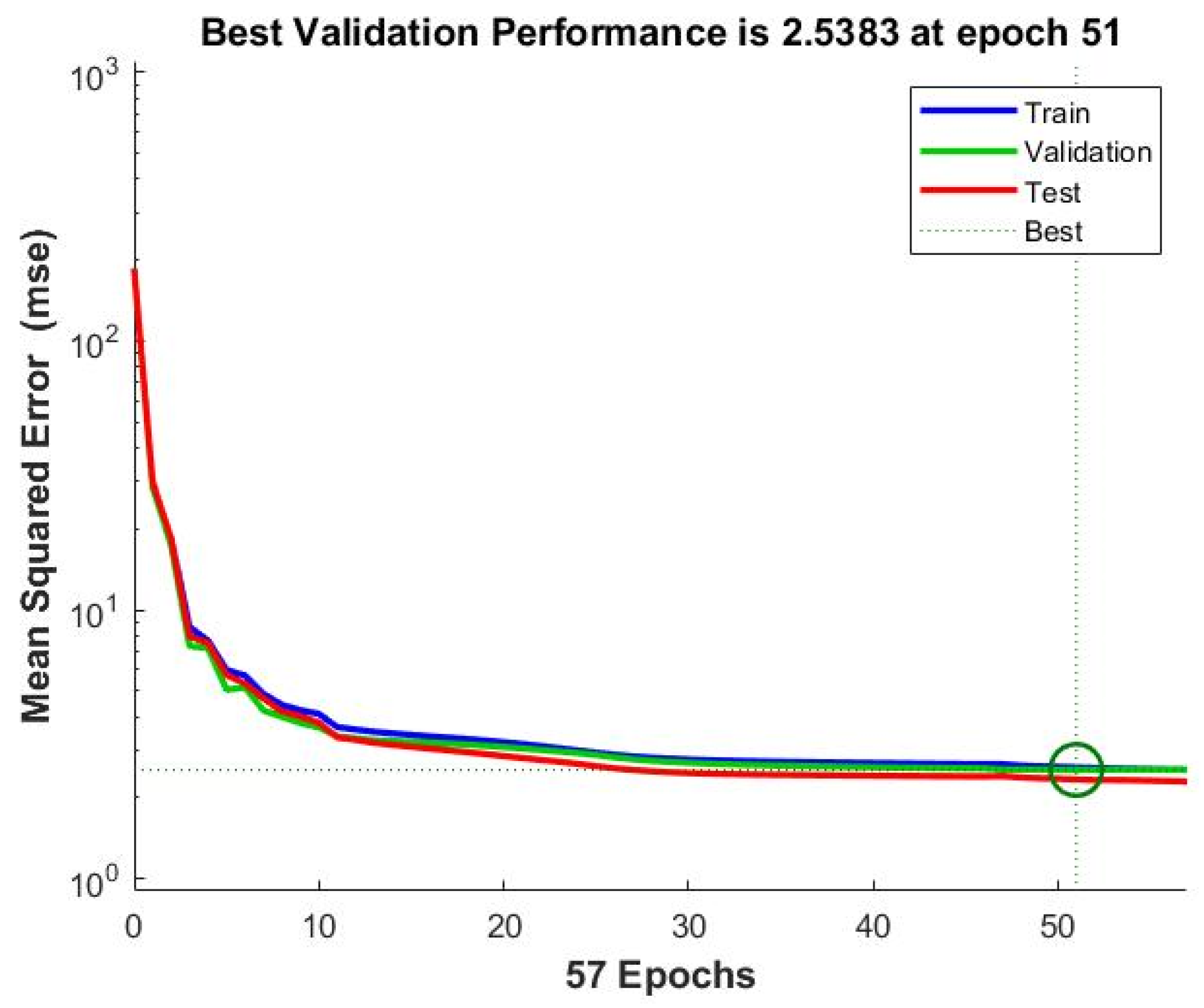
Figure 5 provides a summary of the training process. The best validation performance was achieved at epoch 51 with a mean squared error (MSE) of 2.53 while maintaining low training and testing errors. Regularization techniques were not required due to the relatively small model size and well-curated dataset. Gradient and learning rate behaviors were monitored throughout training to ensure stability. Validation checks were set to trigger early stopping if no improvement was observed after six consecutive epochs.
The trained ANN model was validated using standard performance metrics, and its predictive accuracy was confirmed through comparison with experimental data. The full validation results, including R2 and MSE values, were observed. These findings support the ANN model’s suitability for integration into FE simulation to define the bond–slip interface with high fidelity.
4.3. Mathematical Formulation
The relationships between the inputs and the outputs and the transforming function are typically written as expressed in Equations (2) and (3), respectively. The neural network processes inputs [x
1, x
2, …, xᵢ] through two fundamental mathematical operations. In the first step, each input is multiplied by its corresponding weight, and these products are summed together with a bias term, creating what we call a receive vector y:
Here, [w
1, w
2, …, wᵢ] represents the weights connecting the layers, and b is the bias term. This receive vector y then passes through a transfer function T that shapes the final output:
The bond strength modeling network uses the 5-n-1 architecture, pointing out to the five input nodes [x1, x2, …, x5], n hidden nodes, and one output node. This structure requires two weight matrices: W1 (size n × 5) connecting the input to hidden layer, and W2 (size n × 1) connecting the hidden to output layer. Similarly, it requires two bias terms: b1 (size n × 1) for the hidden layer and b2 (size 1 × 1) for the output layer.
The first layer computation gives us the receive vector y
1 and its corresponding output T
1:
The second layer then processes this output to produce the final receive vector y
2 and output T
2:
The neural network architecture employed a logistic sigmoid activation function exclusively within the hidden layer to introduce nonlinearities, thereby enabling the model to learn complex, nonlinear relationships within the data. The output layer, conversely, utilized a linear activation function to facilitate unbounded prediction of the bond-stress values. Prior to training, the input features were normalized using min–max scaling to ensure a consistent range and improve model convergence, while the target values were deliberately not normalized to allow the network to predict the true, unscaled bond-stress values directly.
4.4. Key Assumptions
The ability of the ANN model to accurately reproduce the experimental bond–slip response is attributed to several key assumptions incorporated during model development:
The bond–slip response is primarily governed by a limited set of influential parameters: It was assumed that the behavior could be characterized by a concise group of experimentally validated inputs, such as surface morphology, embedment length, bar diameter, and concrete compressive strength. Their inclusion ensured that the ANN was trained on physically meaningful predictors.
All input data series follow a consistent loading and slip-measurement protocol: Because each pull-out test was conducted under the same test configuration and instrumentation procedure, the ANN training data represented a uniform measurement framework. This avoided systematic bias and allowed the ANN to generalize the underlying patterns in the full bond–slip curve.
The complete experimental bond–slip curve was used as the target function: The ANN was trained not just on peak values but on the entire bond–slip relationship. This assumes that the bond–slip response is continuous and can be mapped deterministically from the chosen input parameters. This enabled the ANN to capture both ascending stiffness, peak bond stress, and post-peak softening behavior.
The experimental dataset sufficiently represents the variation within each parameter: It was assumed that the range of test data, including multiple surface types, embedment lengths, diameters, and concrete strengths, has provided enough diversity for effective training.
Bond behavior is repeatable under controlled conditions: The ANN assumes that bond failure mechanisms observed in the experiments (pull-out vs. splitting modes) follow consistent patterns driven by the input parameters. As the experimental results demonstrated stable trends, this assumption held and allowed the ANN to learn the nonlinear interactions reliably.
4.5. Model Novelty and Comparison
Unlike previous models that only predict maximum bond strength from a limited dataset, the proposed ANN model uses an extended dataset and provides a continuous bond–slip curve. This enables seamless integration of the model into finite element simulations, where defining the complete stress–slip relationship is essential for bond interface modeling. A comparative summary of the ANN input–output structure and dataset characteristics used in this study versus prior research [
20,
24,
31] is provided in
Table 2.
5. Integration of ANN Model to FE Analysis
5.1. FE Model Creation
5.1.1. Concrete Modeling
Concrete was modeled in ANSYS 2020 R2 using the SOLID65 element, a standard 3D 8-node element capable of representing cracking in tension and crushing in compression. This element is particularly well-suited for the nonlinear modeling of reinforced concrete structures due to its ability to simulate plasticity and post-cracking behavior. The material model was defined using multilinear isotropic properties to capture the stress–strain characteristics under monotonic loading.
5.1.2. Rebar Modeling
GFRP reinforcement bars were modeled using LINK180 elements, which are 3D spar elements with three translational degrees of freedom at each node. Rebar properties were assigned based on test data for a sand-coated bar (
Table 2). While LINK180 does not explicitly represent the surface geometry or ribbing of the bar, this simplification is justified due to the inclusion of bond behavior through external COMBIN39 spring elements, based on ANN predictions. This approach allows for a computationally efficient yet mechanically accurate simulation of the rebar’s interaction with concrete.
5.1.3. Rebar–Concrete Interface Modeling
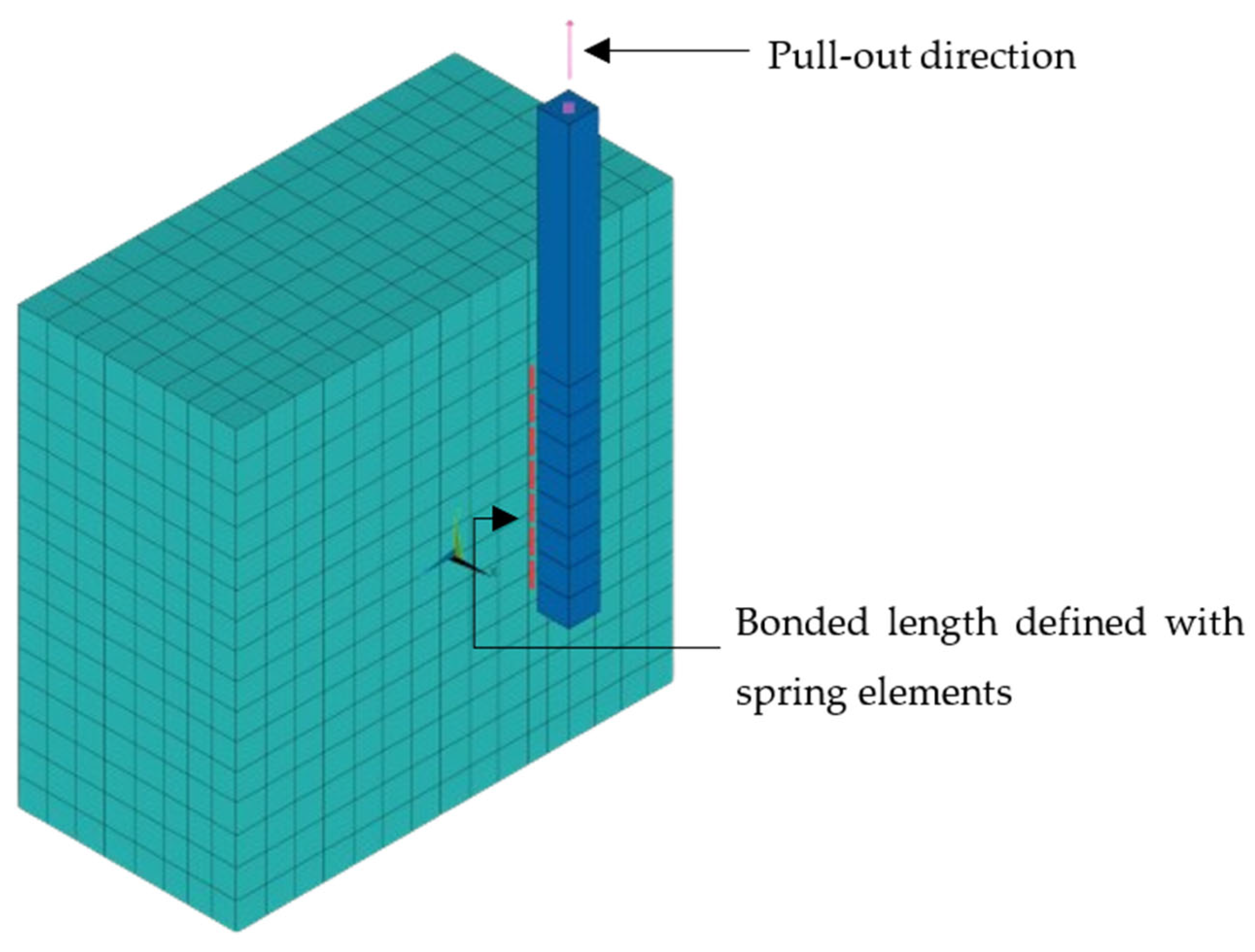
The bond interface between concrete and GFRP reinforcement was modeled using COMBIN39 spring elements (
Figure 6), which possess nonlinear force-deflection capabilities and can be deployed in 1D, 2D, or 3D analyses. The nonlinear spring stiffness was defined using bond–slip curves generated by the ANN model, which predicts bond stress as a function of slip for various geometric and material configurations. It is important to note that these spring elements provide a phenomenological representation of the global bond–slip behavior. They aggregate complex micromechanical interactions, such as chemical adhesion, friction, and mechanical interlock, into a longitudinal response. Consequently, this approach does not explicitly capture radial stresses (dilation) or local rib-scale damage evolution but rather simulates their cumulative effect on load transfer.
5.1.4. Geometric Modeling and Meshing
A bottom-up modeling approach was adopted. Concrete nodes were first generated, followed by the placement of rebar elements at the required positions. Spring elements were inserted between coincident nodes of concrete and rebar elements over the embedded length. To ensure compatibility, the longitudinal mesh of concrete and rebar was configured to have equal spacing, facilitating even spring placement. The use of a loop function in APDL allowed efficient numbering and allocation of the COMBIN39 springs.
5.2. Boundary Conditions and Load Application
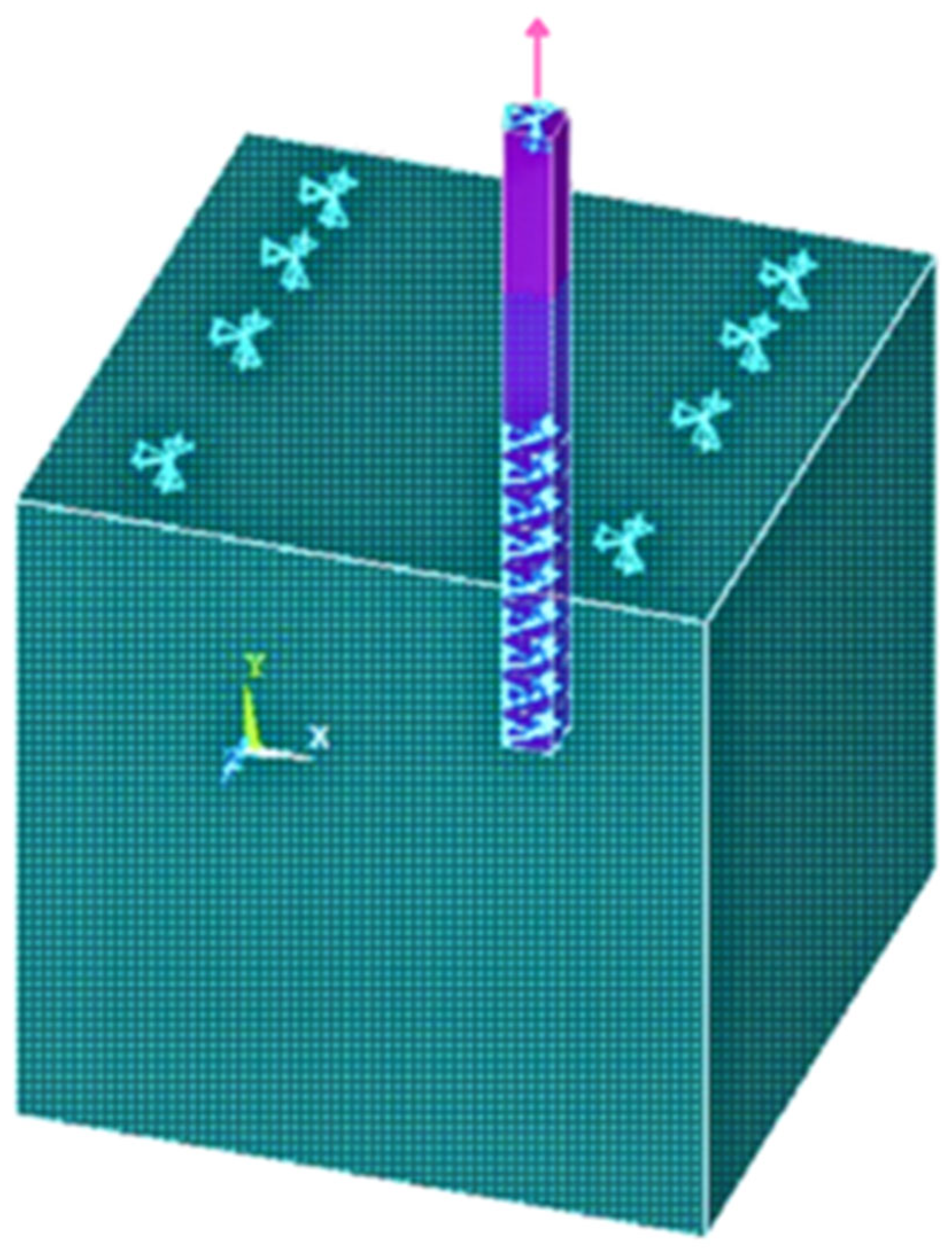
Boundary conditions were defined in line with the experimental pull-out setup, as illustrated in
Figure 7. All translational degrees of freedom (UX, UY, and UZ) were constrained at the bottom face of the concrete cube, while lateral constraints were applied to opposing faces to prevent rotation and ensure a true pull-out response.
Loading was applied as a monotonic displacement-controlled increment at the free end of the rebar. The analysis proceeded under a nonlinear static regime using the Newton–Raphson iterative method. Load increments were automatically adjusted through adaptive time-stepping to maintain convergence. Convergence criteria included both force and displacement tolerances, set to 1% and 5%, respectively.
5.3. Failure Criterion and Post-Processing
In the FE analysis, ultimate failure is broadly defined as the point where the specimen can no longer withstand additional load, corresponding to the sharp load drop observed experimentally. However, in numerical post-processing, this drop is challenging to detect reliably due to solver-induced oscillations. To ensure stable termination, a practical cut-off was adopted: when the load stabilized at an approximately constant value while slip continued to increase (i.e., plateau response), the analysis was stopped at a slip of 5 mm. This plateau phase usually marks the transition from initial bond mobilization to post-peak slip (Stage 2).
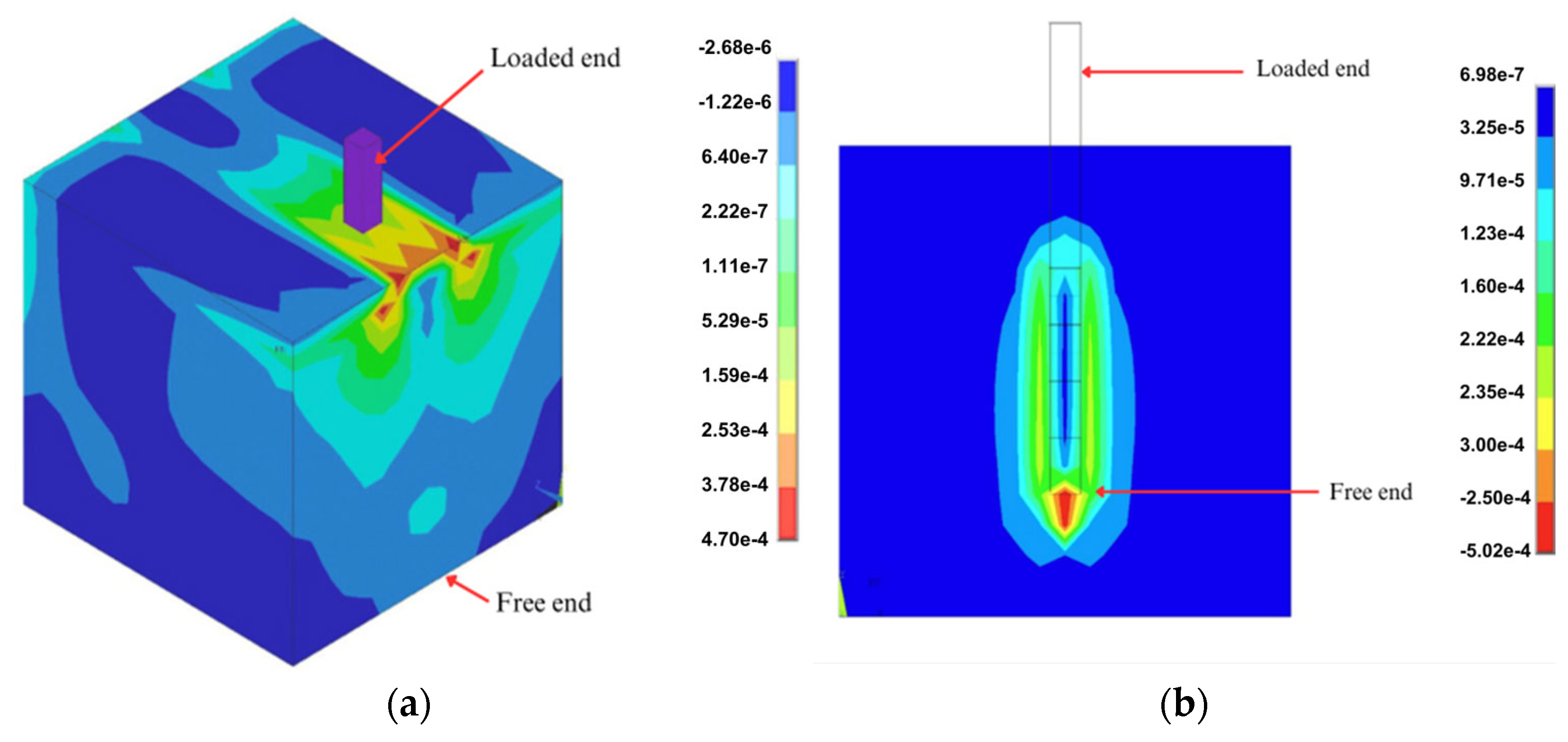
Crack patterns were monitored at each load step by analyzing the principal strain distribution across concrete elements. Special focus was given to the loaded end, where strain localization and initial cracking were expected. The FE-predicted crack patterns were subsequently compared with experimental observations to confirm the model’s accuracy. The FE model then integrated the data-driven ANN bond–slip predictions into a high-fidelity physical simulation, offering insights into the progressive failure mechanisms of GFRP–concrete interfaces under pull-out loading.
6. Results and Discussion
6.1. ANN Model Validation
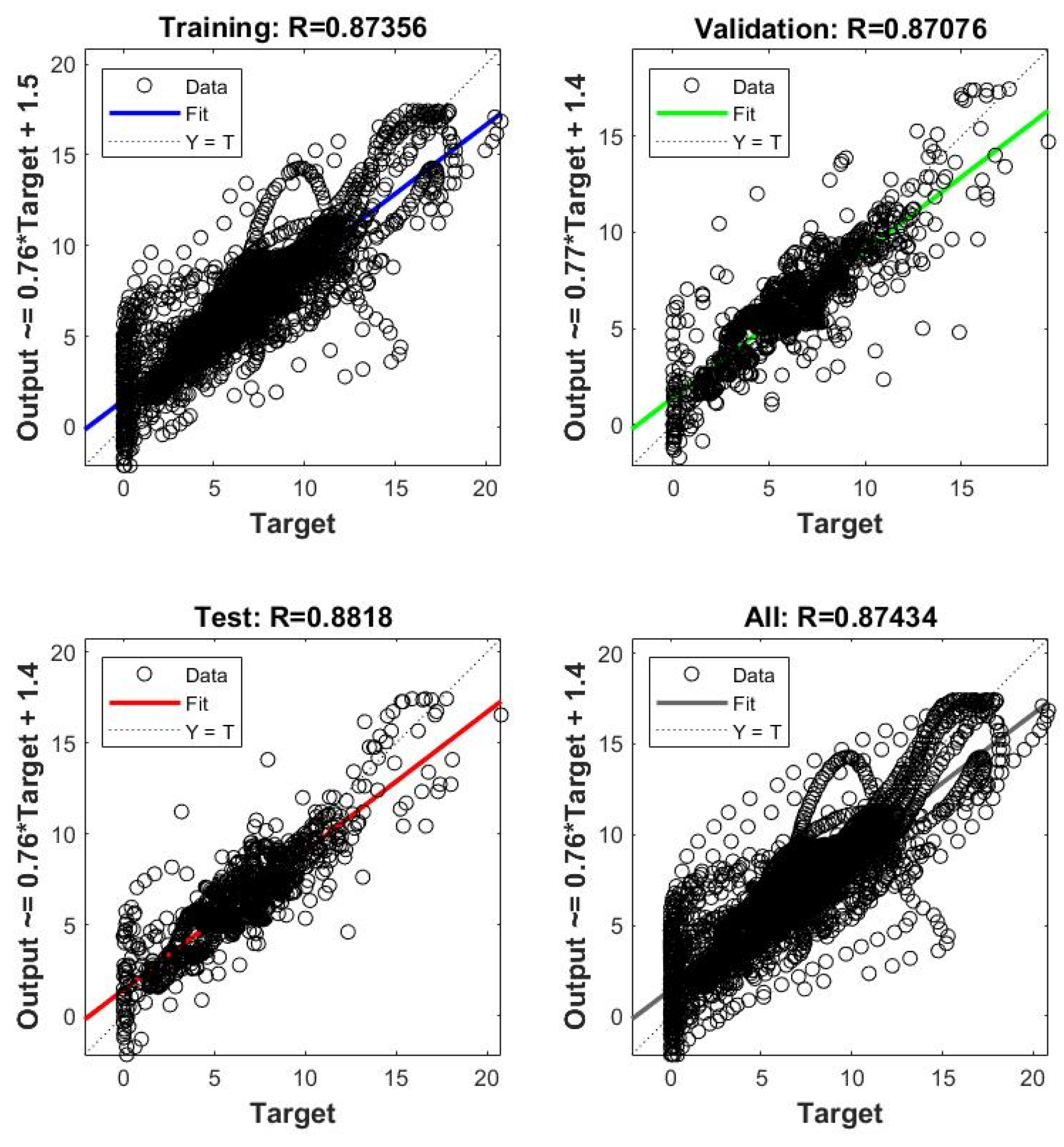
The ANN model was trained on experimental data points covering a range of geometric and material configurations. The predictive power of the trained ANN model is quantitatively substantiated by the regression analysis presented in
Figure 8. The correlation coefficients (R values) between the network’s output and the target values are consistently high across all data subsets: 0.87356 for the training set, 0.87076 for the validation set, and a robust 0.8818 for the independent test set. The overall R value of 0.87434 further reinforces the model’s strong fit. These R values, all exceeding 0.87, indicate a substantial linear relationship between the predicted and actual values, demonstrating the ANN’s capacity to accurately capture the complex, nonlinear underlying patterns within the data.
Figure 9, illustrating the Mean Squared Error (MSE) across epochs, demonstrates that the model achieved its optimal generalization capability at epoch 51, where the validation error reached its minimum of 2.5383. This inflection point is critical, signifying the balance between sufficient learning from the training data and the avoidance of overfitting, a common challenge in neural network development. The training process, as detailed in
Figure 10, further supports this robust performance. The gradient consistently decreased over epochs, stabilizing at 0.67564 by epoch 57, indicating successful convergence of the optimization algorithm. Furthermore, the adaptive learning rate (Mu) maintained stability at 0.001 for a significant duration, and the presence of six validation checks by epoch 57 confirms that the training was effectively halted to preserve the model’s generalization ability, preventing it from memorizing noise in the training set.
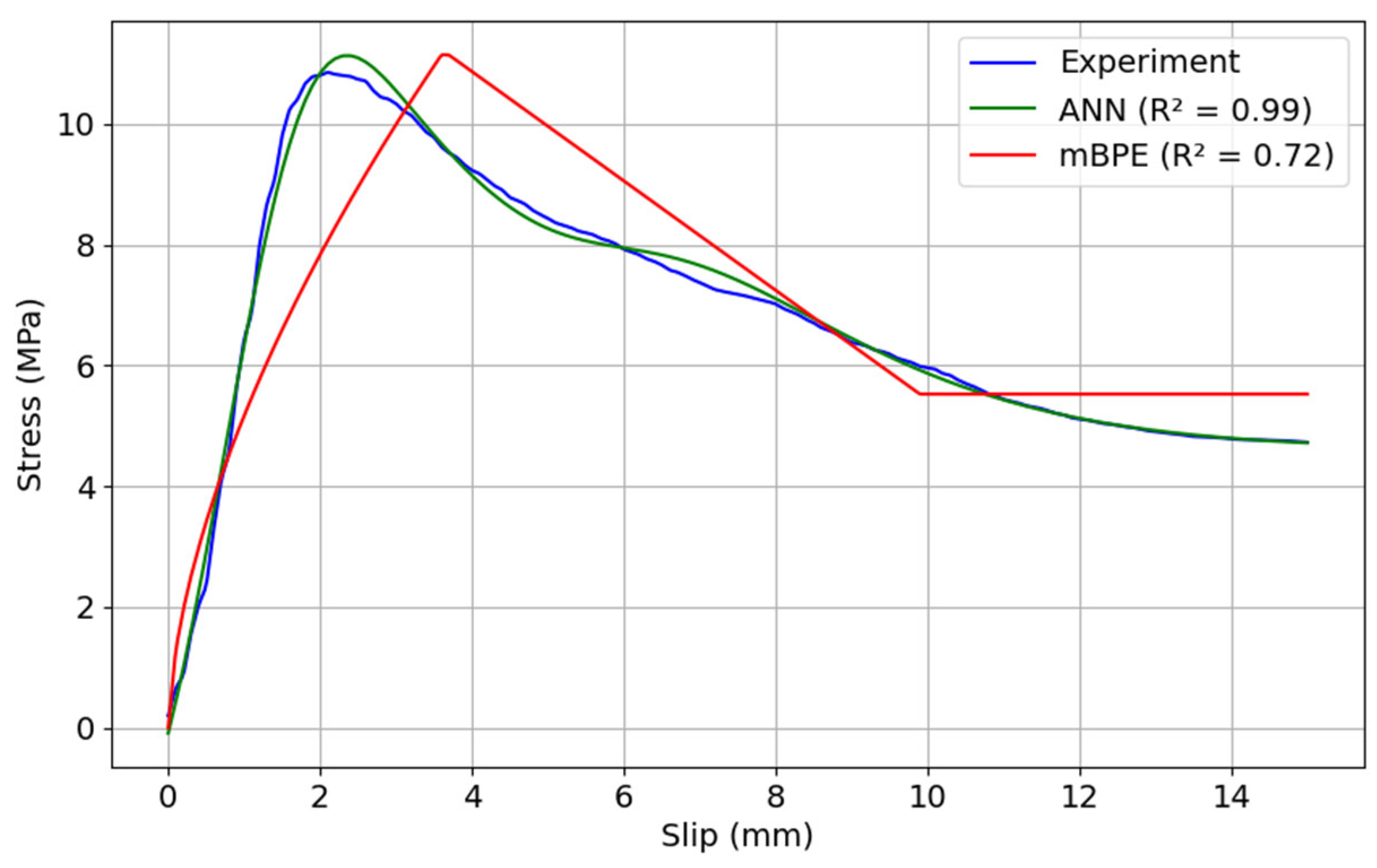
To evaluate the predictive enhancement provided by the ANN model, its output was compared against the modified Bertero–Eligehausen–Popov (mBPE) analytical model.
Figure 11 illustrates the bond–slip responses for the specimen category GS-D12-C40-L72-T42. The mBPE model was able to give a reasonable prediction of the peak bond stress. It underestimated the post-peak behavior and failed to have a good agreement with experimental data, indicating a lower accuracy as reflected by the R
2 value of 0.72.
In contrast, the ANN model showed excellent agreement with the experimental data (R2 = 0.99) over the whole range. It is effective in simulating both the pre- and post-peak stress on the stress–slip curve. This agreement between the model predictions and the experimental data is reflected in the qualitative representation of the full bond–slip response, especially in the post-peak.
6.2. ANN-FEA Simulation Results
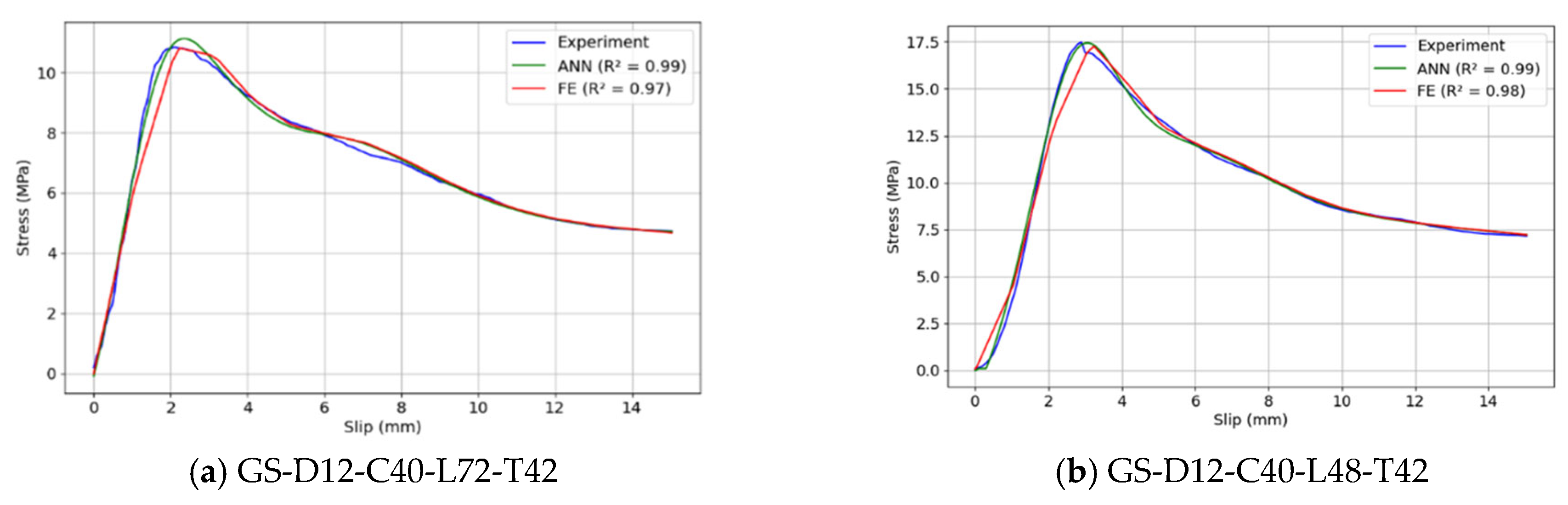
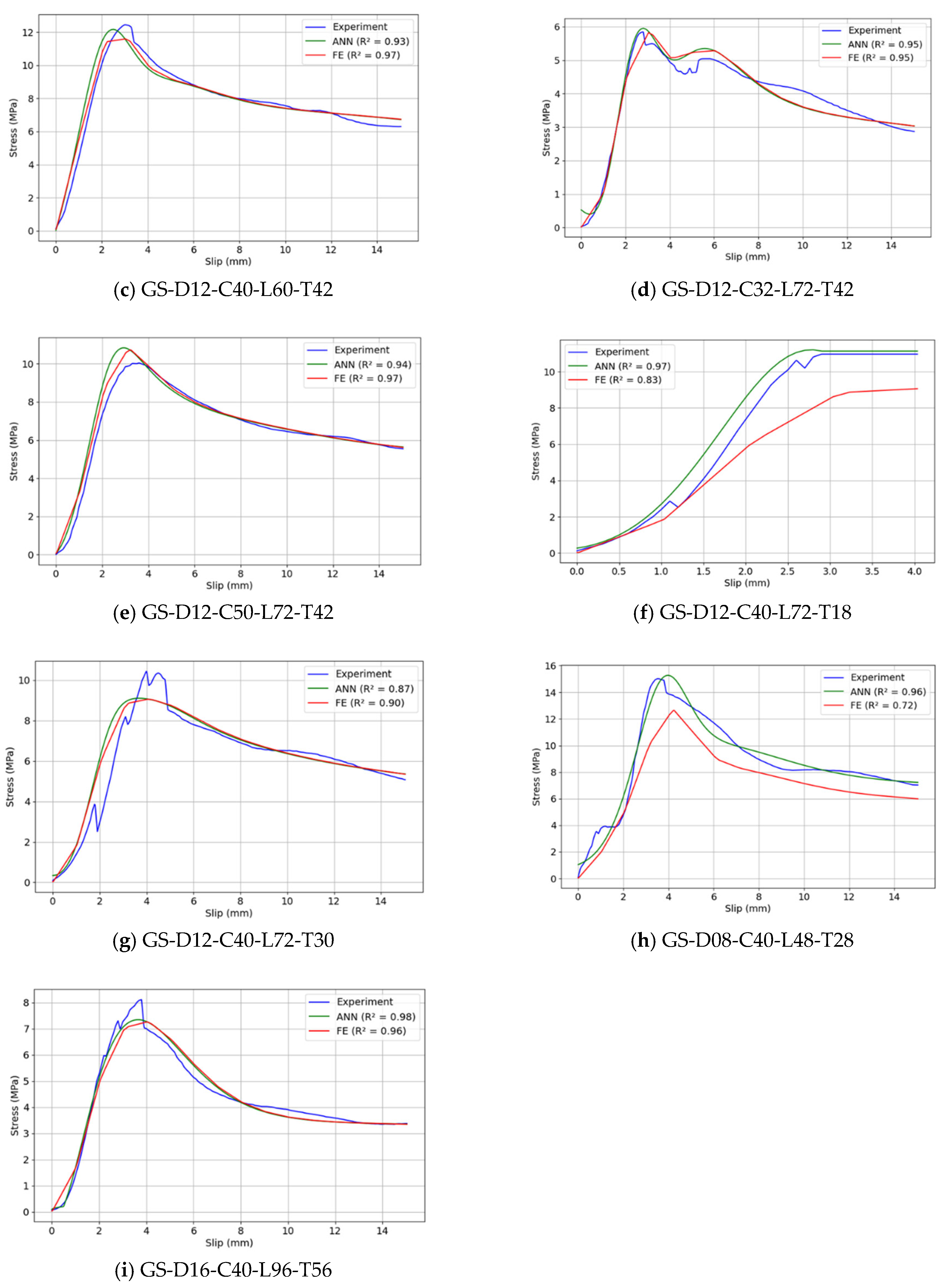
The integrated ANN–FEA model demonstrated excellent predictive capability across all nine specimen configurations, as shown in
Figure 12a–i. Visual comparison with experimental data reveals close agreement in both the ascending and descending branches of the bond–slip curves.
Quantitative analysis shows the model achieved an average R2 value of 0.93 across all cases, with peak bond stress predictions consistently within ±7% of experimental values. The slip at peak stress was predicted with less than 10% error in all configurations. Post-peak softening behavior, often challenging for conventional models, was reliably captured with R2 values exceeding 0.90 for seven of the nine specimens.
Performance varied slightly across parameter ranges, with marginally better accuracy observed for smaller diameter bars (8 mm and 12 mm) compared to 16 mm bars. The model showed particular strength in predicting embedment length effects, maintaining R2 > 0.91 across all length variations. Concrete strength variations (32–50 MPa) were well-handled, though predictions were most consistent at the mid-range 40 MPa strength.
The complete performance metrics for each specimen configuration are presented in
Table 3.
The results confirm the model’s effectiveness in simulating GFRP–concrete bond behavior across a practical range of design parameters. The slight performance reduction for 16 mm diameter bars (7.9% peak stress error) and low-strength concrete (5.6% error for 32 MPa) suggests potential areas for future refinement, though all predictions remain within engineering-appropriate tolerances.
6.3. Strain and Crack Pattern Validation
Figure 13a,b show the principal strain developed in the model’s concrete and bonded area, respectively, during the pull-out simulation. The strain developed during the pull-out process is primarily distributed over the concrete at the loaded end. However, once debonding takes place, the strain distribution becomes more concentrated towards the surface and the free end of the rebar.
These findings are consistent with typical bond failure mechanisms. Moreover,
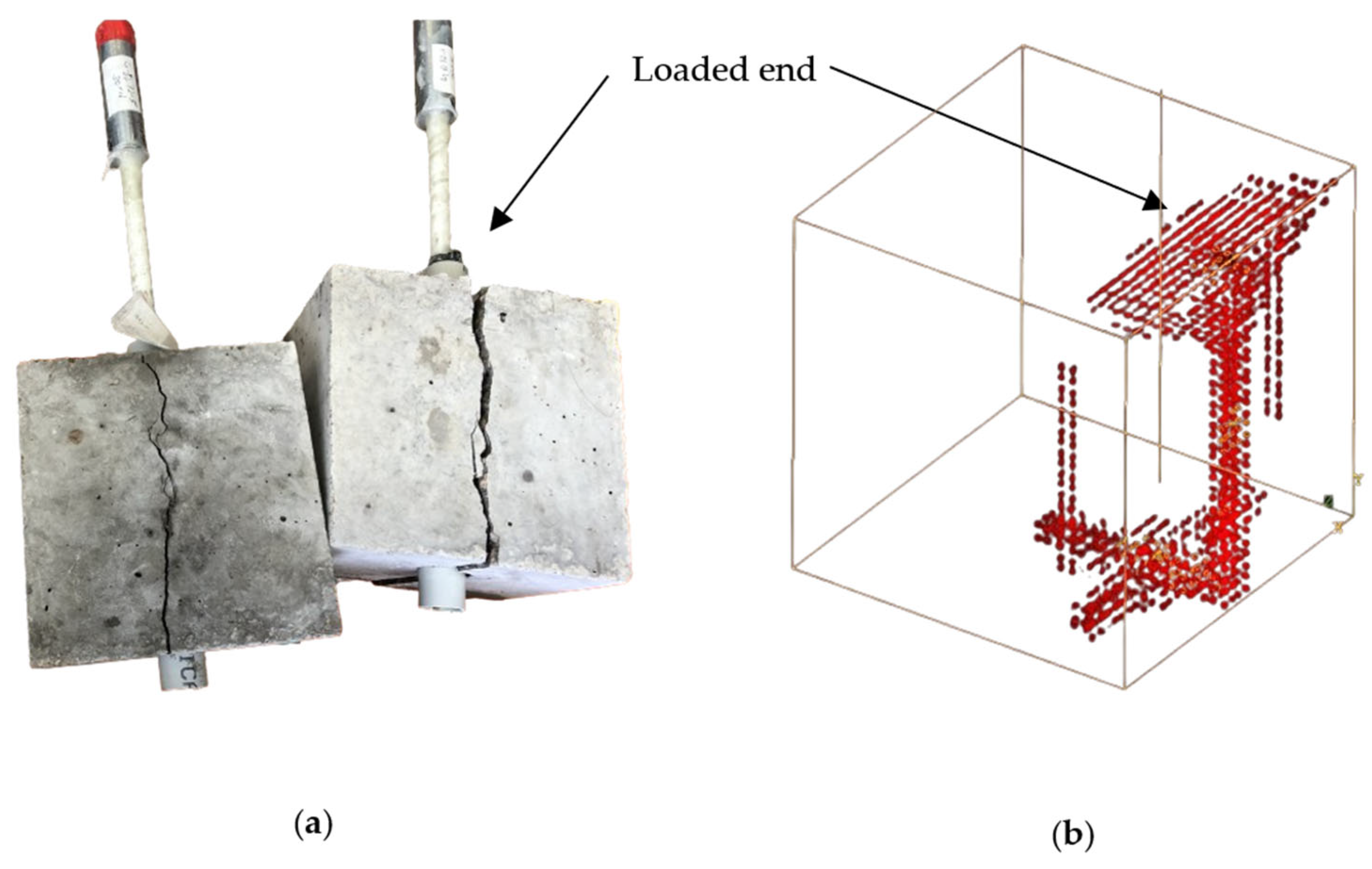
Figure 13a,b compare post-failure cracking in laboratory specimens with the predicted crack patterns from the FE simulation. As the primary strain distribution occurs at the loaded end of the specimen, initial cracks tend to appear on the loaded end face of the concrete cube, and this area also experiences a relatively high density of cracks. This crack development pattern can be observed in
Figure 14a of the laboratory specimen. The FEA model developed by integrating the ANN-based bond model in the simulation (
Figure 14b) predicted the crack pattern consistent with the experimental observation in a laboratory pull-out test.
6.4. Comparison with Non-Bond-Defined FE Simulation
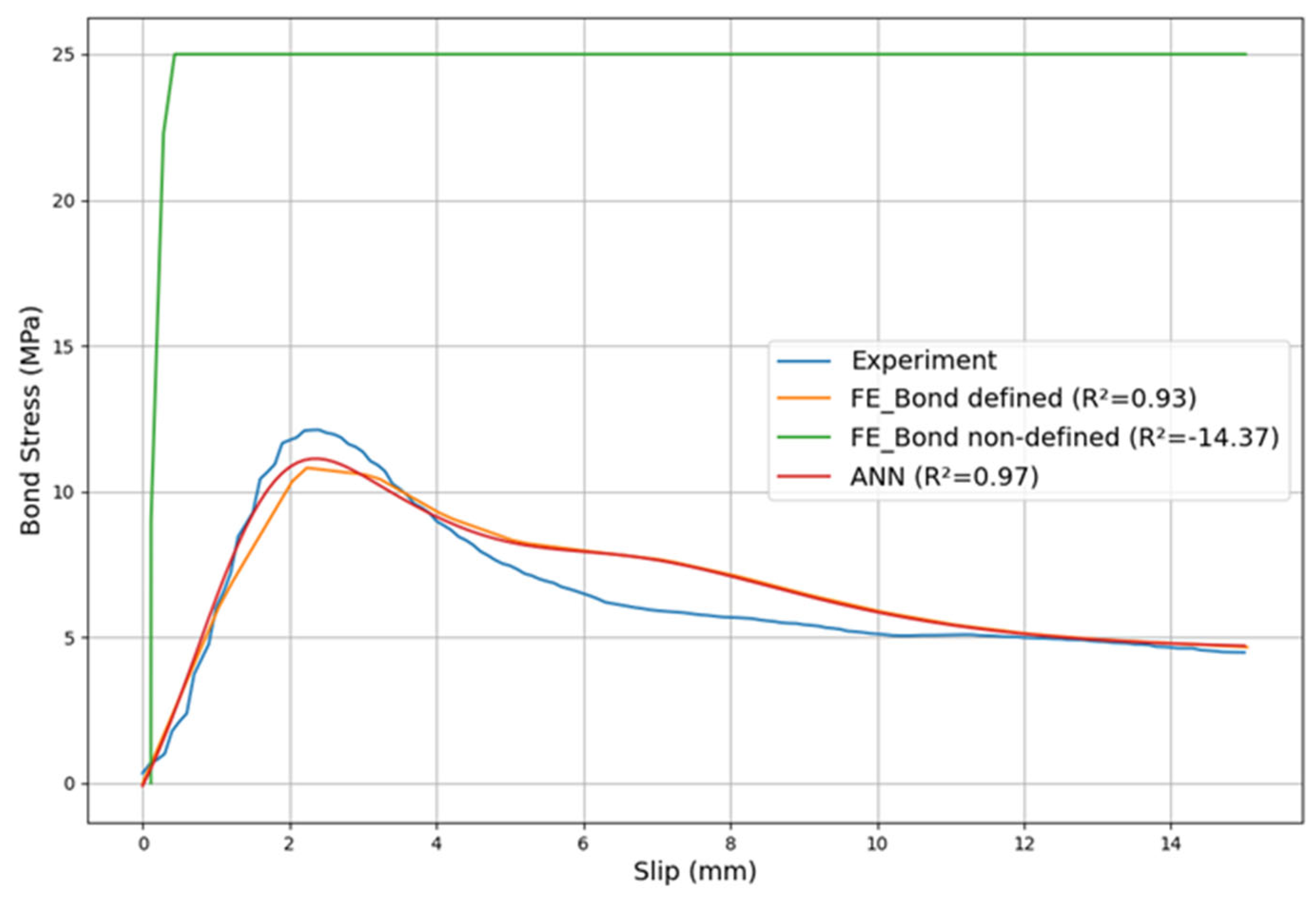
To demonstrate the necessity of explicitly defining bond–slip behavior, a comparative simulation was conducted using the same geometry and material properties (GS-D12-C40-L72-T42) but with a fully bonded interface. The following are shown in
Figure 15:
The non-bond-defined model overestimated peak bond stress.
It failed to capture the descending portion of the bond–slip curve.
Post-peak behavior and slip capacity were significantly misrepresented.
In contrast, the bond-defined FE model achieved an R2 of 0.93 with the experimental result, demonstrating excellent agreement in both peak and post-peak stages. This confirms that integrating the ANN-predicted bond–slip model into the FE simulation provides a critical improvement in the predictive capability of the model presented.
6.5. Parametric Sensitivity and Model Interpretability
To overcome the ‘black box’ limitation of the ANN and assess its engineering interpretability, a sensitivity analysis was conducted to identify dominant input parameters. By analyzing the model’s response to individual parameter variations (consistent with the experimental trends discussed in
Section 3), the following hierarchies of influence were established:
Dominant Parameters (Bar Diameter and Bond Length): The ANN model correctly captures the inverse relationship between bar diameter and bond strength. As observed in the breakdown of prediction accuracy (
Table 3), the model remains robust across diameters but shows higher sensitivity (larger shifts in the stress–slip curve) to changes in diameter and bond length, aligning with the ‘shear lag’ phenomenon where larger diameters/lengths result in non-uniform stress distribution.
Nonlinear Parameters (Concrete Strength): The model successfully reproduces the nonlinear gain in bond strength associated with concrete compressive strength (f’c). Consistent with experimental data, the ANN predicts significant strength gains when increasing f’c from 32 to 40 MPa, with diminishing returns beyond 50 MPa.
Minor Parameters (Cover Thickness): The sensitivity analysis confirms that cover thickness has the lowest weight on the predicted bond–slip curve within the tested range (1.5 D to 3.5 D). The ANN output remains relatively stable against cover thickness variations, matching the experimental observation that confinement provided by the concrete cover was sufficient to prevent splitting failure in most configurations.
This alignment between the ANN’s ‘learned’ parameter weights and established physical mechanisms confirms that the model acts as a reliable predictor rather than a stochastic black box.
7. Conclusions
This study presents a novel hybrid data-driven and computational approach for modeling the bond–slip behavior of GFRP–concrete interfaces by integrating ANN with FE. The key contributions and findings can be summarized as follows:
Advanced Predictive Modeling: A feedforward neural network (FFNN) with optimized architecture (5-n-1) was developed and trained on an extensive experimental dataset (>1000 data points). The ANN model demonstrated exceptional predictive capability while accurately capturing both the ascending and descending branches of the bond–slip response—a significant improvement over conventional models like mBPE with an R2 of 0.72.
Successful FEA Integration: The ANN-derived bond–slip relationships were effectively implemented in FEA through COMBIN39 spring elements, enabling high-fidelity simulation of the interfacial behavior. This integration provided a 2× reduction in prediction errors compared to traditional fully bonded interface models while accurately reproducing crack initiation and propagation patterns observed in experiments.
Comprehensive Validation: The model was rigorously validated against nine independent test cases, showing consistent accuracy across varying parameters (bar diameters 8–16 mm, concrete strengths 32–50 MPa). The ANN–FEA approach achieved an average R2 of 0.93 against experimental bond–slip curves and faithfully replicated observed failure mechanisms.
Practical Implications: This research provides a conceptual and computational framework for incorporating data-driven bond models into FE analysis. The framework establishes the foundation required for future development of simplified design-oriented models and software modules.
Computational Efficiency and Scalability: The proposed framework offers a high-efficiency alternative to detailed micro-modeling by generating ANN-based constitutive curves during pre-processing, thereby eliminating runtime solver latency. By substituting complex 3D interface geometries with reduced-degree-of-freedom spring elements, the method ensures cost-effective scalability from small-scale specimens to full-scale structural components.
8. Limitations and Future Work
While the current model demonstrates excellent performance under monotonic loading conditions, further research should investigate the following:
Extension to cyclic/fatigue loading scenarios
Incorporation of environmental factors (temperature and moisture effects)
Validation for larger bar diameters (>16 mm) and high-strength concrete (>50 MPa)
Application to structural-scale elements (beams and columns)
Validate the spring-based interface method by benchmarking it against high-fidelity 3D Cohesive Zone Models (CZM) and Concrete Damage Plasticity (CDP) to accurately predict splitting failure.
This ANN–FEA framework proposed a new approach for modeling complex interfacial behavior in composite systems, combining the pattern recognition strengths of machine learning with the mechanical rigour of FE analysis. The current model was trained on a single consistent experimental dataset to ensure internal coherence. Future work should incorporate external datasets from independent laboratories to assess the model’s transferability and robustness against variations in test setups.
Author Contributions
Conceptualization, R.D.; Supervision, C.G. and A.O.; Data Curation, R.D., A.O. and C.G.; Writing—Review and Editing, C.G. and A.O.; Writing—Original Draft Preparation, R.D. All authors have read and agreed to the published version of the manuscript.
Funding
This research received no external funding.
Data Availability Statement
The original contributions presented in this study are included in the article. Further inquiries can be directed to the corresponding author.
Conflicts of Interest
The authors declare no conflict of interest.
References
- Zhou, J.; Shang, H.; Huang, Y.; Zhao, W.; Wang, R. Bond properties of GFRP bar embedded in marine concrete subjected to sustained loads. Constr. Build. Mater. 2024, 438, 136982. [Google Scholar] [CrossRef] [Scilit]
- Chen, Y.-D.; Li, P.-D. Anti-corrosion performance of a novel ECC-GFRP spiral-confined RC column. Case Stud. Constr. Mater. 2024, 20, e03241. [Google Scholar] [CrossRef] [Scilit]
- Jafari, A.; Shahmansouri, A.A.; Abdulridha, H.A.; Issa, B.I.; Bengar, H.A. Effect of CFRP confinement on bond-slip behavior of steel rebar in low-strength concrete: Experimentation, prediction and parametric study. Constr. Build. Mater. 2025, 477, 141333. [Google Scholar] [CrossRef] [Scilit]
- ACI PRC 440.1R-15; Guide for the Design and Construction of Structural Concrete Reinforced with FRP Bars. American Concrete Institute (ACI): Farmington Hills, MI, USA, 2015.
- Béton, F.I.D. Externally Bonded Frp Reinforcement for Rc Structures: FIB Buletin 14; International Federation for Structural Concrete: Lausanne, Switzerland, 2001. [Google Scholar]
- Bai, Y.; Ma, Q.; Zhang, Y.; Jin, X.; Han, S. Bond behavior and modeling of steel-FRP composite bars in engineered cementitious composites. Case Stud. Constr. Mater. 2024, 20, e03320. [Google Scholar] [CrossRef] [Scilit]
- La-Hong, H.; Pham, T.M.; Nguyen-Minh, L. Structural behavior of concrete slabs made of seawater sea sand and reinforced with GFRP reinforcement under flexural loading. Structures 2024, 63, 106351. [Google Scholar] [CrossRef] [Scilit]
- de Sá, F.R.G.; Silva, F.d.A.; Cardoso, D.C.T. Tensile and flexural performance of concrete members reinforced with polypropylene fibers and GFRP bars. Compos. Struct. 2020, 253, 112784. [Google Scholar] [CrossRef] [Scilit]
- Kumar, A.; Arora, H.C.; Kumar, K.; Mohammed, M.A.; Majumdar, A.; Khamaksorn, A.; Thinnukool, O. Prediction of FRCM-Concrete Bond Strength with Machine Learning Approach. Sustainability 2022, 14, 845. [Google Scholar] [CrossRef] [Scilit]
- Cosenza, E.; Manfredi, G.; Realfonzo, R. Behavior and modeling of bond of FRP rebars to concrete. J. Compos. Constr. 1997, 1, 40–51. [Google Scholar] [CrossRef] [Scilit]
- Gao, X.; Ren, X.; Li, J.; Zhang, Y. Bond behavior between steel reinforcing bars and concrete under dynamic loads. Struct. Concr. 2018, 19, 1806–1817. [Google Scholar] [CrossRef] [Scilit]
- Rezazadeh, M.; Carvelli, V.; Veljkovic, A. Modelling bond of GFRP rebar and concrete. Constr. Build. Mater. 2017, 153, 102–116. [Google Scholar] [CrossRef] [Scilit]
- Gao, X.; Li, N.; Ren, X. Analytic solution for the bond stress-slip relationship between rebar and concrete. Constr. Build. Mater. 2019, 197, 385–397. [Google Scholar] [CrossRef] [Scilit]
- Gooranorimi, O.; Suaris, W.; Nanni, A. A model for the bond-slip of a GFRP bar in concrete. Eng. Struct. 2017, 146, 34–42. [Google Scholar] [CrossRef] [Scilit]
- Kovačević, M.; Hadzima-Nyarko, M.; Petronijević, P.; Vasiljević, T.; Radomirović, M. Comparative Analysis of Machine Learning Models for Predicting Interfacial Bond Strength of Fiber-Reinforced Polymer-Concrete. Computation 2025, 13, 17. [Google Scholar] [CrossRef] [Scilit]
- Kurtoğlu, A.E.; Anil, Ö.; Çevik, A. A machine-learning-based constitutive bond-slip model for anchored CFRP strips externally bonded on concrete members. Struct. Concr. 2022, 23, 1828–1844. [Google Scholar] [CrossRef] [Scilit]
- Haddad, R.; Haddad, M. Predicting fiber-reinforced polymer–concrete bond strength using artificial neural networks: A comparative analysis study. Struct. Concr. 2021, 22, 38–49. [Google Scholar] [CrossRef] [Scilit]
- Machello, C.; Bazli, M.; Rajabipour, A.; Rad, H.M.; Arashpour, M.; Hadigheh, A. Using machine learning to predict the long-term performance of fibre-reinforced polymer structures: A state-of-the-art review. Constr. Build. Mater. 2023, 408, 133692. [Google Scholar] [CrossRef] [Scilit]
- Shahmansouri, A.A.; Jafari, A.; Bengar, H.A.; Zhou, Y. Steel rebar bond-slip behavior in CFRP-strengthened low-strength concrete: ML-driven solution and reliability analysis. Constr. Build. Mater. 2025, 490, 142302. [Google Scholar] [CrossRef] [Scilit]
- Jafari, A.; Shahmansouri, A.A.; Taslimi, A.; Naser, M.; Zhou, Y. Shear capacity of FRP-RC beams: XML modeling and reliability evaluation. In Structures; Elsevier: Amsterdam, The Netherlands, 2025; p. 110150. [Google Scholar]
- Mahmoudian, A.; Bypour, M.; Kioumarsi, M. Explainable Boosting Machine Learning for Predicting Bond Strength of FRP Rebars in Ultra High-Performance Concrete. Computation 2024, 12, 202. [Google Scholar] [CrossRef] [Scilit]
- Amoako, R.; Jha, A.; Zhong, S. Rock fragmentation prediction using an artificial neural network and support vector regression hybrid approach. Mining 2022, 2, 233–247. [Google Scholar] [CrossRef] [Scilit]
- Shbeeb, N.I.; Katash, A.A.; Oguzmert, M.; Barham, W.S. Estimation of the Bond Strength of Fiber-Reinforced Polymer Bars in Concrete Using Artificial Intelligence Systems. Buildings 2024, 14, 369. [Google Scholar] [CrossRef] [Scilit]
- Nielson, J.; Bhaganagar, K.; Meka, R.; Alaeddini, A. Using atmospheric inputs for Artificial Neural Networks to improve wind turbine power prediction. Energy 2020, 190, 116273. [Google Scholar] [CrossRef] [Scilit]
- Huang, L.; Chen, J.; Tan, X. BP-ANN based bond strength prediction for FRP reinforced concrete at high temperature. Eng. Struct. 2022, 257, 114026. [Google Scholar] [CrossRef] [Scilit]
- Concha, N.C. Neural network model for bond strength of FRP bars in concrete. Structures 2022, 41, 306–317. [Google Scholar] [CrossRef] [Scilit]
- Cascardi, A.; Micelli, F. ANN-Based Model for the Prediction of the Bond Strength between FRP and Concrete. Fibers 2021, 9, 46. [Google Scholar] [CrossRef] [Scilit]
- Ahmad, H.; Elnemr, A.; Ali, N.; Hussain, Q.; Chaiyasarn, K.; Joyklad, P. Finite Element Analysis of Glass Fiber-Reinforced Polymer-(GFRP) Reinforced Continuous Concrete Beams. Polymers 2021, 13, 4468. [Google Scholar] [CrossRef] [Scilit]
- Gouda, A.; El-Salakawy, E. Finite Element modeling of GFRP-reinforced concrete interior slab-column connections subjected to moment transfer. Fibers 2015, 3, 411–431. [Google Scholar] [CrossRef] [Scilit]
- Yang, C.; Kim, Y.; Ryu, S.; Gu, G.X. Prediction of composite microstructure stress-strain curves using convolutional neural networks. Mater. Des. 2020, 189, 108509. [Google Scholar] [CrossRef] [Scilit]
- LX, K.; Wang, B.; PD, H. Prediction of stress–strain behaviors in steels using an integrated constitutive, FEM and ANN model. ISIJ Int. 2001, 41, 795–800. [Google Scholar]
- Allouzi, R.A.; Almasaeid, H.H.; Salman, D.G.; Abendeh, R.M.; Rabayah, H.S. Prediction of Bond-Slip Behavior of Circular/Squared Concrete-Filled Steel Tubes. Buildings 2022, 12, 456. [Google Scholar] [CrossRef] [Scilit]
- Devaraj, R.; Olofinjana, A.; Gerber, C. On the Factors That Determine the Bond Behaviour of GFRP Bars to Concrete: An Experimental Investigation. Buildings 2023, 13, 2896. [Google Scholar] [CrossRef] [Scilit]
- Yan, F.; Lin, Z. Bond behavior of GFRP bar-concrete interface: Damage evolution assessment and FE simulation implementations. Compos. Struct. 2016, 155, 63–76. [Google Scholar] [CrossRef] [Scilit]
Figure 1.
The modified Bertero–Eligehausen–Popov (mBPE) constitutive model representing the bond stress–slip relationship.
Figure 1.
The modified Bertero–Eligehausen–Popov (mBPE) constitutive model representing the bond stress–slip relationship.
Figure 2.
Description of sample designation and configuration.
Figure 2.
Description of sample designation and configuration.
Figure 3.
Pull-out specimen embedded with sand-coated GFRP bar.
Figure 3.
Pull-out specimen embedded with sand-coated GFRP bar.
Figure 4.
Architecture of the ANN model.
Figure 4.
Architecture of the ANN model.
Figure 5.
Neural network training summary.
Figure 5.
Neural network training summary.
Figure 6.
Cross-section of FE pull-out specimen model.
Figure 6.
Cross-section of FE pull-out specimen model.
Figure 7.
Boundary constraints of the FE model.
Figure 7.
Boundary constraints of the FE model.
Figure 8.
Regression plots for training, validation, and testing of the ANN model.
Figure 8.
Regression plots for training, validation, and testing of the ANN model.
Figure 9.
Validation performance of the ANN model.
Figure 9.
Validation performance of the ANN model.
Figure 10.
Training state information.
Figure 10.
Training state information.
Figure 11.
Comparison of mBPE and ANN predictions to the experimental result.
Figure 11.
Comparison of mBPE and ANN predictions to the experimental result.
Figure 12.
(a–i). Comparison of bond-stress–slip response from ANN prediction and FE simulation to experimental data.
Figure 12.
(a–i). Comparison of bond-stress–slip response from ANN prediction and FE simulation to experimental data.
Figure 13.
Principal strain distribution. (a) Principal strain at concrete; (b) principal strain at bonded area.
Figure 13.
Principal strain distribution. (a) Principal strain at concrete; (b) principal strain at bonded area.
Figure 14.
Cracked specimens after maximum load application for the representative specimen GS-D12-C40-L72-T42. (a) Laboratory specimen; (b) FEA Model.
Figure 14.
Cracked specimens after maximum load application for the representative specimen GS-D12-C40-L72-T42. (a) Laboratory specimen; (b) FEA Model.
Figure 15.
Comparison of FE bond defined and non-defined predictions.
Figure 15.
Comparison of FE bond defined and non-defined predictions.
Table 1.
Parameters and Variables.
Table 1.
Parameters and Variables.
| Investigated Parameters | Corresponding Variables |
|---|
| Bar Diameter (mm) | Embedment Length (mm) | Concrete Strength (MPa) | Cover Thickness (mm) |
|---|
| Bar Diameter | 8 | 48 | 40 | 28 |
| 12 | 72 | 40 | 42 |
| 16 | 96 | 40 | 56 |
| Embedment Length | 12 | 48 | 40 | 42 |
| 12 | 60 | 40 | 42 |
| Concrete Strength | 12 | 72 | 32 | 42 |
| 12 | 72 | 50 | 42 |
| Cover Thickness | 12 | 72 | 40 | 18 |
| 12 | 72 | 40 | 30 |
Table 2.
ANN model development in the current study vs. existing studies.
Table 2.
ANN model development in the current study vs. existing studies.
| | ANN Model Training | ANN Prediction Output |
|---|
| Inputs | Output | No. of Data Points |
|---|
| Existing studies | Bond-influencing parameters | Maximum bond strength | <400 | Maximum bond strength |
| Current study | Bond-influencing parameters + bond–slip | Bond stress corresponding to bond slip | >1000 | Bond–slip behavior including maximum stress |
Table 3.
ANN–FEA model performance for tested specimen samples.
Table 3.
ANN–FEA model performance for tested specimen samples.
| Figure Reference | Specimen ID | R2 Value | Peak Stress Error (%) | Slip at Peak Error (%) | Post-Peak R2 |
|---|
| 12a | GS-D12-C40-L72 | 0.94 | 3.2 | 5.1 | 0.93 |
| 12b | GS-D12-C40-L48 | 0.95 | 2.8 | 4.7 | 0.94 |
| 12c | GS-D12-C40-L60 | 0.93 | 4.1 | 6.3 | 0.91 |
| 12d | GS-D12-C32-L72 | 0.91 | 5.6 | 7.8 | 0.89 |
| 12e | GS-D12-C50-L72 | 0.92 | 4.9 | 6.5 | 0.9 |
| 12f | GS-D12-C40-L72-T18 | 0.90 | 6.2 | 8.1 | 0.88 |
| 12g | GS-D12-C40-L72-T30 | 0.93 | 3.9 | 5.7 | 0.92 |
| 12h | GS-D08-C40-L48-T28 | 0.96 | 2.3 | 3.9 | 0.95 |
| 12i | GS-D16-C40-L96-T56 | 0.89 | 7.9 | 9.2 | 0.86 |
| Disclaimer/Publisher’s Note: The statements, opinions and data contained in all publications are solely those of the individual author(s) and contributor(s) and not of MDPI and/or the editor(s). MDPI and/or the editor(s) disclaim responsibility for any injury to people or property resulting from any ideas, methods, instructions or products referred to in the content. |