


Abstract
Coastal erosion is a growing concern along many Mediterranean sandy coasts, particularly where reduced fluvial sediment supply, relative sea-level rise and coastal development coincide. This study uses multi-mission Landsat 5/7/8/9 and Sentinel-2 data in Google Earth Engine to extract long-term shoreline series (1984–2025) from MNDWI-based composites. DSAS-style metrics quantify multi-decadal change, while a supervised linear regression forecasting model—validated against a 2013 orthophoto and an independent 2017–2025 test set using an RMSE-based acceptance criterion—is employed to forecast shoreline positions up to 2050. Using this framework, we reconstruct and forecast shoreline evolution along the ~38 km Ionian coast of Basilicata (southern Italy), a microtidal, sediment-starved littoral that has been affected by significant erosion over the past few decades, threatening natural habitats, infrastructure and economic activities. Results show pervasive erosion over the last four decades, with an average shoreline retreat of ≈47 m along the entire coast, and localized retreats exceeding 400 m, particularly at the mouths of the Agri and Sinni rivers and near the Metaponto sector. Forecasts, under linearity and trend-persistence assumptions, indicate further substantial retreat by 2050 in already critical sectors. Methodologically, this work provides a reproducible framework to inform scenario-based coastal planning in similar Mediterranean environments and the first multi-decadal, spatially continuous satellite-based analysis and machine learning-supported forecast for the Basilicata coast, offering a robust basis for regional coastal management.
1. Introduction
Coastal zones are among the most dynamic and fragile environments on Earth [1], where natural and anthropogenic processes interact across a wide range of spatial and temporal scales [2,3,4]. Globally, 24% of sandy beaches erode at rates exceeding 0.5 m/yr, while 28% accrete and 48% remain stable, with erosion hotspots concentrated in densely populated regions [5]. The Mediterranean basin is a recognized climate change “hotspot”, particularly vulnerable to sea-level rise (SLR), increased storm frequency, and sediment starvation [6,7]. Here, the combination of extreme marine weather events, long-term SLR, and extensive human modification of fluvial systems has amplified shoreline retreat and geomorphological instability along many microtidal sandy coasts [8].
At the national scale, Italy exemplifies the cumulative impacts of climatic and anthropogenic forcing. Approximately 18% of its low-lying coastline has eroded in recent decades, with southern regions such as Basilicata, Apulia, and Calabria among the most severely affected [9,10]. Projections indicate that by 2050, nearly 70% of Italian sandy beaches will experience significant retreat under ongoing SLR scenarios, threatening tourism infrastructure and coastal ecosystems [8]. These trends pose increasing challenges for coastal risk management, particularly in low-lying coastal plains where intensive land use and reduced sediment supply constrain natural accommodation space and limit the range of feasible adaptation strategies [11,12,13].
Zooming in to the regional level, the Ionian coast of Basilicata in southern Italy is a paradigmatic case of accelerated coastal change in a microtidal (<0.4 m), sediment-starved setting [14]. This ~38 km stretch between the Bradano and Sinni river mouths forms a low-lying coastal plain characterized by narrow sandy beaches, low dune ridges and multiple river mouths opening into the Gulf of Taranto. Historical analyses reveal a shift from a progradational phase (1870–1954), driven by high fluvial sediment supply from the Sinni, Agri, Cavone, Basento and Bradano rivers, to a pronounced erosive phase after the 1950s [15,16]. This transition has been mainly attributed to drastic sediment-flux reduction caused by dam construction (e.g., San Giuliano, Monte Cotugno, Pertusillo), gravel mining, land-use changes and urban development along the coastal plain. For instance, the Bradano River’s mean discharge dropped from ~10.5 m3/s before 1960 to <3 m3/s, with suspended sediment load reduced by nearly an order of magnitude [17]. Recent analyses using Sentinel-1 SAR imagery indicate shoreline retreats of up to ≈60 m along segments of the Ionian Basilicata coast between 2015–2021, highlighting dominant erosive processes in the area [18]. Local subsidence in deltaic zones (2–5 mm/yr; [19]) further exacerbates relative SLR, enhancing beach lowering and shoreline retreat, but plays a secondary role compared with the dominant influence of sediment deficit and wave-driven coastal erosion.
Recent sedimentological and morpho-evolutionary studies in the Policoro and Metaponto areas document significant shoreline retreat and morphological transformations in both emerged and submerged beach sectors [14,16]. Aerial photographs and bathymetric data over the last century indicate a net regression of several hundred metres near the Sinni River mouth, linked to sediment deficit and subsidence [15]. Seasonal monitoring reveals strong beach-width variability and submerged-bar migration, particularly during winter storms [14]. Coastal vulnerability assessments confirm medium-to-high risk levels for erosion and marine flooding along the Ionian Basilicata coast [17,20], where low-lying coastal plains host intensive agriculture, tourist resorts and linear infrastructure. Despite regional planning efforts, mitigation remains limited, with hard structures (e.g., groynes, seawalls) often providing local benefits but inducing downdrift erosion [14].
Given this background, a comprehensive understanding of the spatio-temporal evolution of coastal erosion along the Ionian coast of Basilicata is essential for both scientific investigation and coastal management. Although several studies have analysed shoreline dynamics in other Italian and Mediterranean regions using diverse methods, including aerial photogrammetry, GNSS surveys, LiDAR and sub-pixel extraction from Landsat or Sentinel-2 imagery [10,17,21,22], few have focused specifically on the Basilicata coast, despite its well-documented vulnerability and environmental importance. Previous works on this littoral system have mostly relied on localized geomorphological surveys or on discrete temporal datasets (e.g., [15,16,20]), offering valuable information that this study extends to a long-term, spatially consistent perspective.
Moreover, high-resolution and sub-pixel approaches have demonstrated their potential for accurate shoreline extraction in Mediterranean microtidal environments: on a Spanish test site, Pardo-Pascual et al. (2018) [22] reported mean horizontal errors on the order of 3–4 m with standard deviations of about 5–6 m for shorelines derived from Landsat 7/8 and Sentinel-2 using SWIR bands, which outperformed NIR-based extractions, especially under whitewater conditions. However, most published applications of these techniques have been designed as detailed experiments on a limited number of sites and over relatively short time windows, rather than as long, coast-length reconstructions. In southern Italy, and along the Ionian Basilicata coast in particular, their use within multi-decadal, spatially consistent shoreline-monitoring frameworks is still essentially unexplored. Against this backdrop, there is clear scope for systematic, low-cost and reproducible approaches that exploit open satellite archives to provide continuous multi-decadal evaluations of shoreline change and support coastal planning decisions.
In parallel, the last decade has seen rapid growth in the availability of free multi-mission satellite archives and cloud computing platforms for large-scale coastal monitoring [23,24]. The Landsat program and the Sentinel-2 mission offer radiometrically stable, multi-spectral imagery suitable for shoreline detection [25,26], while Google Earth Engine (GEE) enables efficient processing of long time series of surface reflectance data [27,28]. Spectral water indices such as the Normalized Difference Water Index (NDWI; [29]) and SWIR-based variants such as the Modified Normalized Difference Water Index (MNDWI; [30]), combined with automated thresholding schemes, have been widely used for semi-automatic extraction of land–water boundaries from high-resolution imagery, with demonstrated accuracies compatible with regional-scale applications [31,32].
At the same time, machine learning has increasingly been applied to coastal and environmental problems, from shoreline detection and classification [33,34] to the prediction of erosion–accretion patterns [35,36], providing flexible tools to exploit long observational records and quantify uncertainty in a data-driven way. However, for the Ionian Basilicata coast, multi-decadal satellite-derived shoreline series have not yet been coupled with an explicit forecasting framework and a quantitative, alongshore-resolved assessment of model skill, despite the existence of similar satellite-based shoreline analyses in other Mediterranean settings (e.g., [37,38]).
In this context, the present study builds on previous regional work but extends it in several directions. In operational terms, we (i) exploit multi-mission Landsat (5/7/8/9) and Sentinel-2 data to reconstruct a 42-year time series (1984–2025) of annual shoreline proxies extracted from MNDWI-based composites in GEE, (ii) compute DSAS-style (Digital Shoreline Analysis System-style) shoreline-change metrics [39] along a dense set of cross-shore transects, and (iii) develop a supervised linear machine learning model that is explicitly trained and tested at the transect scale before being used to forecast shoreline positions up to 2050. Although the shoreline forecasts produced here are not yet combined with detailed land-use layers for a full exposure analysis, they provide a spatially continuous, scenario-based picture of potential retreats and advances that can be readily intersected with existing datasets such as CORINE Land Cover [40] in future work.
Within this overall framework, the specific objectives of the study are to:
- reconstruct the multi-decadal evolution of the shoreline along the Ionian coast of Basilicata over the period 1984–2025 by integrating Landsat and Sentinel-2 surface-reflectance data;
- quantify the spatial patterns of erosion and accretion using DSAS-style statistics (net shoreline movement, endpoint rate, linear regression rate) computed along 752 cross-shore transects spaced every 50 m and relate these patterns to river mouths, coastal structures and municipal boundaries to identify erosional hotspots and relatively stable sectors;
- develop and validate a machine learning-based linear forecasting model that learns per-transect trends from the 1984–2016 observations, evaluates predictive skill over 2017–2025 through an RMSE-based acceptance criterion grounded in an explicit positional-uncertainty budget, and then produces annual shoreline forecasts for up to 2050 for all non-rigid segments of the coast;
- discuss the implications of the reconstructed trends and 2050 projections for coastal risk and management along the Ionian Basilicata littoral, with particular reference to the widespread presence of bathing establishments, low-lying agricultural land and other exposed assets, in the broader context of Italian and Mediterranean erosion scenarios [9,17,20,41].
In doing so, this research provides a region-wide, multi-decadal and spatially continuous analysis of shoreline evolution along the Basilicata coast using freely available multi-mission satellite data, coupled, for the first time, with an explicitly validated forecasting scheme. The contribution is twofold: methodologically, it presents a reproducible workflow that integrates open satellite archives, automated shoreline extraction and interpretable, transect-scale forecasting with explicit train–test validation; regionally, it delivers a consistent, multi-decadal, coast-length reconstruction and projection for a highly vulnerable Mediterranean microtidal, sediment-starved littoral.
2. Materials and Methods
This section describes the complete workflow adopted in this study, from multi-mission satellite image pre-processing and shoreline extraction in Google Earth Engine (GEE) [42,43] to the computation of shoreline-change statistics and the construction of linear forecasts in Python 3.13.7. An overview of the main processing steps and their implementation environment is provided in Figure 1.
Figure 1.
Schematic workflow of the methodology adopted in this study. The procedure combines (i) multi-mission satellite and orthophoto data acquisition; (ii) annual image pre-processing, compositing and automated shoreline extraction in GEE; (iii) computation of DSAS-style shoreline-change metrics and train–test validation of a linear forecast model in Python; and (iv) reconstruction and representation of observed (1984–2025) and forecasted (2026–2050) shorelines back in GEE. The grey box indicates input datasets, blue boxes indicate processing steps implemented in GEE, and orange boxes indicate processing steps implemented in Python.
2.1. Study Area
Basilicata is a predominantly rural region in southern Italy where agriculture remains a key land use and economic sector, while beach-based tourism along the Ionian coast represents a key socio-economic asset. In recent years, regional stakeholders have increasingly supported technological innovation in agriculture and the strengthening of the coastal tourism system [44,45,46,47,48,49,50]. The study area encompasses ~38 km of the Ionian Basilicata coastline, delimited by the regional boundaries with Calabria (SE) and Apulia (NW), and including the river-mouth sectors of the Sinni, Agri, Cavone, Basento and Bradano rivers. This coastal stretch, facing the Gulf of Taranto, is part of the wider Metapontum coastal plain, one of the most active sedimentary systems in the central Mediterranean. Administratively, it includes the coastal municipalities of Bernalda (Metaponto), Pisticci, Scanzano Jonico, Policoro, Rotondella, and Nova Siri (Figure 2).
Figure 2.
Study area. Location of the Basilicata region (southern Italy; inset) and the investigated Ionian coastal sector. The black outline denotes the Basilicata regional boundary, whereas the red outlines delineate the coastal municipalities intersecting the coastal sector.
Morphologically, the Basilicata coast is a low-lying sandy littoral bounded inland by a gently undulating hinterland composed of Pleistocene and Holocene alluvial deposits of the Bradanic Trough, an intermontane basin bordered by the Apennine chain to the west and the Murgian carbonate plateau to the east [51]. The shoreline is interrupted by the mouths of the Sinni, Agri, Cavone, Basento, and Bradano rivers, whose alluvial fans have historically supplied most of the sediment to the coastal zone [15,52]. The beaches are composed of fine- to medium-grained quartz–feldspathic sands in the north and coarser lithoclastic sediments in the south; small foredune ridges are locally preserved but have been extensively degraded by erosion and human activities [16].
The wave climate of the Ionian Sea is characterized by moderate energy and a dominant southeast–southwest wind regime that generates most of the storm events affecting the Basilicata coast. Significant wave heights commonly range between 0.25 and 2.5 m, occasionally exceeding 3 m during winter storms [17]. The tidal regime is microtidal, with a mean tidal range of 0.20–0.45 m [15]; therefore, wave and surge events, rather than tides, control most of coastal morphodynamics. The climate is thermo-Mediterranean, with an average annual temperature above 16 °C and annual precipitation below 500 mm, concentrated in autumn and winter [17].
Human pressure has profoundly modified the morphodynamics of this coastal system. Since the 1950s, the construction of large reservoirs, such as San Giuliano, Monte Cotugno, and Pertusillo, and widespread gravel mining from riverbeds have drastically reduced the sediment load delivered to the sea. At the same time, the development of tourism infrastructure, coastal roads, and harbours (e.g., Porto degli Argonauti in the Pisticci sector and the Marina di Policoro/Marinagri complex) has altered longshore sediment transport, enhancing localized erosion [20]. These interventions have led to a sharp transition from a historical phase of coastal accretion (1870–1950) to a modern phase of generalized erosion, with shoreline retreat rates locally exceeding 2–5 m/yr near river mouths [15,17].
From a land-use perspective, the Ionian Basilicata coast is mostly devoted to seaside tourism, with a dense alternation of bathing establishments and public beaches interrupted only by short stretches near river mouths and harbour inlets. Seasonal beach facilities, camping sites and beach clubs occupy much of the back-beach zone, often backed by coastal pine forests and agricultural land. In several municipalities, especially in the Metaponto and Scanzano Jonico sectors, repeated erosion crises have led to a progressive loss of usable beach width, forcing operators to relocate or dismantle structures and prompting emergency nourishment campaigns and new shore-protection works [14,17,53,54]. This combination of limited sediment input, low coastal relief, intense anthropogenic disturbance and heavy touristic use makes the Ionian Basilicata coast highly vulnerable to marine flooding and long-term shoreline retreat. Consequently, this area has been identified by national and regional authorities as a priority zone for coastal risk management in southern Italy [55,56], representing an ideal case study for assessing historical and contemporary coastal dynamics in the Mediterranean context.
2.2. Satellite and Ancillary Data
To reconstruct the multi-decadal evolution of the shoreline, we used 42 annual snapshots covering the period 1984–2025, derived from multi-mission optical satellite imagery. The core dataset consists of Level-2 surface reflectance products from the Landsat 5 TM, Landsat 7 ETM+, Landsat 8 OLI and Landsat 9 OLI-2 sensors and from the Sentinel-2A/B MSI sensor, accessed through the GEE data catalogue [57]. Landsat collections provide a 30 m spatial resolution and a 16-day nominal revisit, effectively reduced to 8 days since the launch of Landsat 9 in 2021, thanks to the joint operation of Landsat 8 and 9. Sentinel-2 Level-2A surface reflectance data offer a spatial resolution of 10 m in the visible–NIR bands and 20 m in the SWIR bands, with a 5-day revisit. Sentinel-2 imagery was incorporated from 2017 onwards to enhance the spatial detail of recent years.
Figure 3 provides context on satellite data used in this study, showing (a) the spatial coverage of the Sentinel-2 MGRS tiles and Landsat WRS-2 scene footprints intersecting the study area and (b) the annual number of images employed by sensor, highlighting the continuity of the Landsat archive and the increased sampling density since 2017 with the addition of Sentinel-2.
Figure 3.
(a) Spatial coverage of Sentinel-2 (MGRS) and Landsat (WRS-2) footprints over the study area, with municipal boundaries and the Basilicata region outline. (b) Annual number of satellite images by sensor (Landsat 5/7/8/9 and Sentinel-2) over 1984–2025.
To minimize the influence of clouds and short-term storm impacts, we relied exclusively on Level-2 surface reflectance products and applied the mission-specific cloud and cloud-shadow masks (Landsat QA_PIXEL and Sentinel-2 SCL). For each year, all available cloud-free observations over the study area were assembled into a multi-sensor image collection, from which a single annual composite was derived by computing the per-pixel median surface reflectance (see Section 2.3 for details). In all cases, the relevant spectral bands (Blue, Green, Red, SWIR1) were resampled to a common 10 m grid matching the Sentinel-2 B2 projection in order to obtain harmonized multispectral stacks suitable for shoreline detection. Harmonising Landsat reflectance to the native 10 m Sentinel-2 grid, either through spatial resampling or cross-sensor adjustment, is increasingly adopted in multi-mission Landsat–Sentinel-2 products to stabilise long-term surface reflectance series and improve the consistency of derived spectral indices and biophysical variables [58], including in Mediterranean coastal settings [59]. The 10 m grid is used here for geometric co-registration and for building a consistent multi-sensor stack, but it should not be interpreted as an increase in the effective spatial detail of the historical record. In particular, pre-2017 composites remain constrained by the native Landsat sampling (30 m).
High-resolution airborne data were used exclusively for validation of the automatically extracted shorelines. In particular, we exploited the 2013 regional orthophoto mosaic provided by the Basilicata spatial data infrastructure (RSDI [60]) and an associated vector shoreline of the same year. Both datasets were co-registered to the 2013 satellite-derived coastline and sampled along the same set of cross-shore transects used in the subsequent analysis. The design of the validation experiment and the associated metrics are described in Section 2.5, while the resulting accuracy figures are reported in Section 3.1 and discussed in Section 4.1.
All datasets were handled in the WGS 84/UTM Zone 33N coordinate system, which provides a locally quasi-Cartesian metric reference frame suitable for computing alongshore distances and cross-shore displacements.
2.3. Image Pre-Processing and Annual Composites in Google Earth Engine
All image pre-processing and compositing steps were implemented in the Google Earth Engine environment. For each year between 1984 and 2025, we built a multi-sensor, cloud-free annual mosaic over the study area, which was then used as the basis for shoreline extraction.
Landsat Level-2 surface reflectance collections were first harmonised by applying the mission-specific scaling factors provided by the USGS and selecting a common set of spectral bands (Blue, Green, Red, SWIR1). Cloud and cloud-shadow contamination was removed using the QA_PIXEL quality band by masking out all pixels flagged as clouds, cloud shadows or adjacent cloud-affected pixels. Sentinel-2 Level-2A imagery was ingested from the COPERNICUS/S2_SR_HARMONIZED collection and masked using the Scene Classification Layer (SCL). In this case we retained only clear-sky surface classes (dark features, vegetation, bare soil and water), which effectively removed clouds and their shadows. No additional land–water or land-cover masks were applied at this stage, so the subsequent shoreline detection fully relied on spectral water indices rather than on prior land/sea delineations.
For each year, all available cloud-free Landsat and Sentinel-2 observations over the region of interest were merged into a single multi-sensor ImageCollection. From this collection, we generated one annual composite by computing, on a per-pixel basis, the median of the surface reflectance values in each band. This per-pixel median mosaic effectively filtered out outliers associated with individual storms, turbid plumes or anomalous sea-state conditions and provided shoreline proxies that were representative of typical wave and tidal levels over the entire year. In the same way, any episodic, short-lived inundation affecting low-lying coastal sectors within a given year was expected to influence only a limited subset of observations and was therefore largely suppressed by the annual per-pixel median compositing. To ensure spatial consistency across sensors, all composites were resampled to a common 10 m grid using the Sentinel-2 B2 band as a reference. Landsat images, originally at 30 m, were first converted to floating point and then resampled with bilinear interpolation to the Sentinel-2 projection (WGS 84/UTM Zone 33N, 10 m pixel size). The resulting annual mosaics therefore share a harmonised set of spectral bands (Blue, Green, Red, SWIR1) and a common spatial resolution of 10 m, which greatly simplifies the subsequent computation of the Modified Normalized Difference Water Index (MNDWI) and the automated shoreline extraction described in Section 2.4. Although this bilinear resampling could reduce staircase artefacts and discretisation noise and propagate contextual spectral information from neighbouring pixels [61], it did not increase the effective spatial detail of the Landsat sensors and may have blurred land–water transitions or slightly shifted strong gradients. Accordingly, resampling was used only for harmonization, and uncertainty/validation were interpreted in sensor-native terms (30 m spatial resolution).
An analogous pre-processing workflow was adopted to derive a dedicated composite for the 2013 validation experiment, with the only difference that, in that case, the multi-sensor collection was restricted to images acquired in July–August 2013 in order to match the acquisition period of the regional orthophoto over the Ionian Basilicata sector (see Section 2.5).
2.4. Automated Shoreline Extraction
Shorelines were extracted automatically from the annual cloud-free composites described in Section 2.3 by means of water–land classification based on the Modified Normalized Difference Water Index (MNDWI). For each yearly mosaic, we computed the MNDWI as
where ρGreen and ρSWIR1 are surface reflectances in the green and shortwave-infrared bands, respectively. In sandy coastal environments, MNDWI enhances the spectral contrast between water, wet sand and dry beach, making it suitable for extracting a radiometrically defined land-water boundary from multispectral imagery [62,63,64]. When applied to annual cloud-free composites, the resulting polyline should be interpreted as an ‘effective’ yearly waterline proxy—representative of the typical position of the land–water radiometric contrast over that year and less sensitive to short-lived fluctuations (e.g., run-up/foam or brief inundation)—rather than an instantaneous, tide-referenced or morphodynamic shoreline indicator.
To focus the analysis on the coastal zone and avoid spurious contributions from inland water bodies, the MNDWI image was first clipped to a narrow coastal buffer encompassing the investigated shoreline sector. Within this coastal strip, we applied a global automatic threshold based on Otsu’s method [65], which identified the MNDWI value that maximized the between-class variance of the two resulting clusters. Pixels with MNDWI values above the threshold were classified as “water”, whereas pixels below the threshold were classified as “land”. Transitional or periodically flooded zones (e.g., near river mouths) were not treated as a dedicated class; instead, the workflow was designed to extract the open-coast shoreline by subsequently retaining only the largest connected water body (Ionian Sea) and discarding inland/disconnected water patches. No ancillary land–sea masks were used at this stage: the land–water separation was entirely driven by the spectral response encoded in MNDWI.
Otsu thresholding on a single water index can be sensitive when the land–water histogram departs from a clear two-class structure, particularly under strong class-proportion imbalance (e.g., when the target occupies a small fraction of the study area) [66] and/or in muddy, intertidal settings where silty mudflats and tide-dependent shoreline configurations introduce spectrally ambiguous transitions at the land–sea interface [67], for which multi-index decision rules and frequency/time-series logic have been proposed to better represent intermittently inundated surfaces [68].
In our case, the analysis targeted a predominantly sandy, microtidal coastline and the threshold was estimated within a narrow coastal strip designed to include both beach and nearshore waters, and the resulting sample was characterised by a moderate land–water proportion (≈70% land and ≈30% water; ~165,000 Landsat-scale pixels). This configuration reduced the likelihood of the extreme imbalance scenario and provided sufficient variability of terrestrial surfaces for stable separation while retaining an extensive sea sample.
The initial binary water mask could contain narrow connections between the open sea and river channels or harbour basins or artificially dredged inlets, as well as small, noisy features. To remove these artefacts while preserving the main sea body, we applied a morphological opening (erosion followed by dilation) using a circular structuring element. Specifically, we set a minimum preserved channel width Wmin = 150 m and used a circular kernel with radius equal to half of this value. Erosion (implemented as a local minimum filter) removed thin connections, and the subsequent dilation (implemented as a local maximum filter) restored the remaining water body. This procedure removed water links narrower than approximately 150 m, breaking undesired links between the open sea and river or port inlets while maintaining the overall coastline geometry (Figure 4a).
Figure 4.
Post-processing of the MNDWI–Otsu water mask and sea-polygon selection. (a) Examples of morphological opening used to remove narrow, spurious water connections at the Agri River mouth and the Policoro harbour inlet. (b) Example annual composite (2025) over the coastal strip and corresponding sea polygon extracted (outlined in yellow) from the cleaned water mask, retaining only the largest contiguous water body (Ionian Sea) for shoreline delineation.
From the cleaned water mask, vector polygons were generated. For each polygon, the surface area was computed, and only the largest contiguous water body—corresponding to the Ionian Sea—was retained, while smaller inland water bodies were discarded. The shoreline for each year was then defined as the interface between the retained “sea” polygon and the surrounding land (Figure 4b).
To reduce the influence of pixel-scale crenulations and minor planform irregularities unrelated to genuine coastal morphology, the raw shoreline polylines were subsequently simplified using the built-in ‘simplify’ method of the Earth Engine geometry API, which implements the Douglas–Peucker algorithm [69]. We adopted a maximum positional error of 20 m, which acted as a tolerance on the displacement of the simplified line with respect to the original geometry. This value was selected as a practical, pixel-scale compromise: it was close to the characteristic geometric deviation associated with a 30 m Landsat pixel (=30/√2 ≈ 21 m), thus avoiding an overly aggressive simplification, while still being large enough to suppress raster-induced stair-step oscillations at scales of ~1–2 pixels of the working grid (10 m). At the same time, the chosen tolerance was consistent with the adopted reference positional uncertainty (σref = 15 m; Section 2.5), so it mainly suppressed raster-induced “zig-zag” artifacts while preserving the overall shoreline position and curvature (Figure 5).
Figure 5.
Example of the Douglas–Peucker simplification applied to the extracted shoreline, shown as a smoothed polyline (red) over the 2025 annual composite in the Pisticci Marina–Basento River mouth–Metaponto Lido sector.
The simplified shorelines were finally stored in the GEE asset repository and used as input for the baseline definition and cross-shore transect analysis described in Section 2.6.
2.5. Design of Shoreline Validation Against the 2013 Orthophoto
An independent validation experiment was carried out to quantify the horizontal accuracy of the satellite-derived shorelines and define a reference positional uncertainty to be used in the subsequent forecast evaluation. For this purpose, we exploited the only high-resolution aerial dataset currently available for the study area in the regional geoportal, namely, the 2013 regional orthophoto mosaic provided by the Basilicata spatial data infrastructure (RSDI [60]; ground sampling distance ~0.2 m), together with an associated vector shoreline of the same year. The orthophoto tiles covering the Ionian Basilicata coast were reprojected to the WGS 84/UTM Zone 33N coordinate system and mosaicked into a single raster (Figure 6).
Figure 6.
A 2013 orthophoto mosaic of the Ionian coast downloaded from the Regional Spatial Data Infrastructure (RSDI [60]) geoportal and corresponding 2013 reference shoreline (blue line).
To ensure temporal consistency between the satellite-derived and orthophoto shorelines, we produced a dedicated 2013 composite restricted to the period of the aerial survey. Specifically, a multi-sensor image collection was built by selecting all cloud-free Landsat and Sentinel-2 Level-2 scenes acquired over the study area between July and August 2013, in line with the flight dates of the orthophoto over the south-eastern quadrant that included the Ionian coast. This collection was processed with the same pre-processing workflow described in Section 2.3 (cloud masking and per-pixel median compositing), and the shoreline for 2013 was then extracted using the automated MNDWI-based procedure outlined in Section 2.4, including the same morphological filtering and geometric simplification.
The comparison between the orthophoto-derived and satellite-derived 2013 coastlines was carried out along the same set of cross-shore transects used in the multi-decadal analysis [70]. For each transect, we computed the signed cross-shore distance between the intersection point with the orthophoto shoreline and the intersection point with the satellite shoreline. The resulting set of cross-shore offsets was then analysed statistically by computing the mean signed bias and the standard deviation of the distribution.
Because transects crossing rigid coastal structures (e.g., groynes, harbour jetties) or river mouths can yield extreme cross-shore offsets that are not representative of the typical detection accuracy, we adopted a trimmed-statistics approach. In particular, we discarded the outer tails of the distribution and focused on the central portion containing the vast majority of transects (96% of the data), which effectively removed the most extreme outliers while preserving the overall behaviour of the shoreline detection method. The numerical results of this comparison (mean bias, standard deviation and trimmed percentiles) are reported in Section 3.1 and discussed in Section 4.1.
On the basis of this validation and consistent with the ground sampling distance of the Landsat sensors, we adopted a conservative reference horizontal uncertainty of σref = 15 m, approximately corresponding to half a Landsat pixel. This value was intentionally larger than the scatter observed in the 2013 comparison and was used as a global benchmark for the positional accuracy of all satellite-derived shorelines. In the following, σref serves as a scaling parameter in the definition of the maximum acceptable RMSE on the test period for the linear forecast model (Section 2.7.2).
2.6. Baseline and Cross-Shore Transects
The multi-decadal shoreline analysis was carried out in a baseline–transect framework, following a DSAS-style approach. The reference baseline was defined as the satellite-derived shoreline for 1984, after the MNDWI-based extraction, morphological filtering and geometric simplification described in Section 2.3 and Section 2.4. Cross-shore transects were generated at regular alongshore intervals of 50 m along the baseline. A 50 m transect spacing is commonly adopted in DSAS-based regional shoreline-change assessments on sandy coasts, providing a practical balance between resolving alongshore variability and keeping the transect set manageable for quality checking; the same spacing is used in several USGS National Shoreline Change datasets (e.g., [71,72,73,74]). Given that the 1984 Ionian Basilicata coast is nearly rectilinear at the scale of the study area, all transects were oriented consistently in the same offshore direction. Each transect was implemented as a straight line centred on the baseline (Figure 7).
Figure 7.
Analysis geometry along the Ionian coast of Basilicata, showing the 1984 baseline shoreline (red) and the cross-shore transects spaced at 50 m alongshore (blue).
For every annual shoreline between 1984 and 2025, the intersection with each transect was computed. When multiple intersections occurred, which happened only where transects crossed rigid coastal structures (such as groynes or harbour jetties), we retained the landward-most intersection point. This choice ensured that, in the case of multiple intersections including structure and back-beach, each transect sampled the effective shoreline position and provided a single, well-defined cross-shore position per transect and year. For each transect–shoreline intersection, the cross-shore distance between the baseline and the annual shoreline was calculated along the transect direction, with positive values indicating a landward shift and negative values indicating a seaward retreat. The resulting dataset consisted of a long table of baseline–shoreline distances as a function of year and alongshore position, which formed the basis for the computation of shoreline-change statistics and the construction of the linear forecasts described in Section 2.7.
2.7. Shoreline-Change Metrics and Machine Learning-Based Linear Forecasting Model
The time series of cross-shore distances described in Section 2.6 were used to compute standard shoreline-change metrics and calibrate, at each transect, a simple machine learning model for shoreline forecasting in the form of a supervised linear regression. In this framework, each transect corresponded to an individual regression task where the annual cross-shore distances d(t) were treated as the target variable and time t as the predictor. The resulting models were trained on historical data, validated on an independent test period, and then used to generate shoreline projections up to 2050.
Let d(t) denote the signed cross-shore distance between the 1984 baseline and the shoreline position at year t, measured along the transect direction, with positive values indicating a landward shift (erosion) and negative values indicating a seaward shift (accretion). For each transect, the sequence d(t) for t between 1984 and 2025 was analysed to derive both end-point and trend-based indicators of shoreline change and fit a linear model that was later exploited for forecasting (Section 2.7.2 and Section 2.7.3).
2.7.1. DSAS-Style Shoreline Change Statistics (1984–2025)
To characterise multi-decadal shoreline change along the Ionian Basilicata coast, we adopted a set of DSAS-style metrics computed independently for each transect over the full observational period 1984–2025.
First, we evaluated the net shoreline movement (NSM), defined as the difference between the cross-shore distance at the end (2025) and at the beginning (1984) of the observation period along a given transect. Positive NSM values indicate erosion, whereas negative values denote accretion. Second, we computed the end point rate (EPR) of shoreline change, defined as the NSM divided by the time interval between the two end points. The EPR therefore expresses the average rate of shoreline displacement, in metres per year, over the 41-year period 1984–2025. Third, we derived a trend-based estimate of shoreline change by fitting a simple linear regression model to the annual cross-shore distances d(t) as a function of time t. For each transect, we approximated d(t) with a straight line of the form
where a is the intercept and b is the linear regression rate (LRR), which represents the best-fitting constant rate of shoreline change over 1984–2025 in metres per year. Positive values of b indicate a long-term erosional trend, whereas negative values indicate long-term accretion. Together with the regression slope, we computed the standard error of b and its two-sided 95% confidence interval, which provided a measure of the statistical significance and robustness of the inferred trend.
All metrics were calculated from the same set of annual cross-shore distances. The resulting NSM, EPR and LRR values, together with their confidence intervals, provide a compact description of spatial patterns of shoreline retreat and advance along the Ionian Basilicata coast and serve as a benchmark against which the linear forecasts to 2050 can be interpreted.
2.7.2. Train–Test Validation of the Supervised Linear Forecast Model
For each transect not affected by rigid coastal structures, we evaluated the performance of the supervised linear regression model within a machine learning framework based on a temporal train–test split. The available observational period 1984–2025 consisted of 42 annual shoreline positions. We used the first 80% of the series (33 years, from 1984 to 2016) as the training set and the remaining 20% (9 years, from 2017 to 2025) as the test set. Transects intersecting only rigid structures (such as groynes and harbour jetties, with no intersection with the adjacent beach) were excluded from the modelling step and treated separately in the forecasting procedure (Section 2.7.3).
For each non-rigid transect, we considered the annual cross-shore distances d(t) between the 1984 baseline and the shoreline position at year t, with positive values indicating landward shifts and negative values indicating seaward retreats (Section 2.6). A straight line of the form was fitted to the training subset (1984–2016) by ordinary least squares, where b represents the linear rate of shoreline change (in metres per year) and a is the intercept. To minimise spurious vertical offsets between the fitted line and the observed time series at the transition between training and test, the intercept was reparameterized so that the regression line matches the observed shoreline position at the last training year (2016). This anchoring ensures continuity between the fitted model and the recent observational record.
Model performance was assessed on the independent test period 2017–2025. For each transect, the linear model was used to predict shoreline positions for the test years, and the root mean square error (RMSE) between observed and predicted cross-shore distances was computed. To decide whether the linear model yielded an acceptable predictive skill at a given transect, the test-period RMSE was compared with a transect-specific maximum acceptable RMSE, denoted RMSEmax. This threshold combined a fixed term related to the reference positional uncertainty of the shoreline and a term proportional to the expected shoreline displacement over the test interval:
Here, σref = 15 m is a conservative reference horizontal uncertainty, approximately corresponding to half a Landsat pixel and consistent with (but slightly larger than) the scatter inferred from the 2013 validation experiment (Section 2.5). The factor k1 = 2 defines a tolerance envelope of 2σref ≈ 30 m, which intentionally exceeds the intrinsic positional uncertainty to implicitly account for additional, unmodelled sources of variability such as tidal excursions, wave setup, interannual changes in sea level and the effects of shoreline simplification. The second term involved the absolute value of the training slope b and the duration of the test period Ttest = 9 years. The coefficient k2 = 0.20 scaled this contribution, making the threshold slightly more permissive where larger shoreline displacements were expected over the test interval, while keeping it stricter in quasi-stable sectors. A simple sensitivity check using plausible ranges of k1 and k2 (k1 = 2.0 ± 0.2 and k2 = 0.20 ± 0.10) produced only minor changes in the set of accepted transects and did not alter the spatial pattern of the main erosional hotspots.
For each transect, we then computed the ratio r between the test-period RMSE and the corresponding threshold:
and used this scaled error to classify the forecast quality. Transects with r ≤ 2/3 were labelled as “good”, those with 2/3 < r ≤ 1 as “medium”, and those with r > 1 as “bad”. The forecast was accepted for subsequent use only for transects in the “good” or “medium” classes. This classification provided a spatially explicit assessment of where the linear model could be considered reliable enough to support shoreline projections to 2050 and where additional caution or alternative treatments were required (Section 2.7.3).
2.7.3. Construction of 2026–2050 Shoreline Forecasts
The machine learning-based linear forecasting model described in Section 2.7.2 was ultimately used to generate annual shoreline projections for the period 2026–2050 at each transect. The procedure distinguished between (i) non-rigid transects where the linear model passed the RMSE-based quality test, (ii) non-rigid transects where the model was rejected, and (iii) transects intersecting rigid coastal structures.
For non-rigid transects with accepted forecasts (“good” or “medium” class according to the scaled RMSE criterion), the final prediction was based on a linear fit using all available observations between 1984 and 2025. For each such transect, the annual cross-shore distances were regressed against time by ordinary least squares, yielding a slope and intercept that summarise the long-term trend over the full observation period. As in the training step, the intercept was reparameterised so that the fitted line passes exactly through the last observed shoreline position (2025), thereby anchoring the forecast to the most recent measurement. This final linear model was then extrapolated in time to compute predicted shoreline positions for each year from 2026 to 2050, expressed as cross-shore distances from the 1984 baseline. For non-rigid transects where the linear model did not meet the RMSE-based acceptance criterion (“bad” class), shoreline forecasts were obtained by alongshore interpolation from neighbouring accepted transects. Transects intersecting only rigid coastal structures were not subjected to linear modelling. For these “rigid” transects, shoreline projections for 2026–2050 were obtained by simply maintaining the last observed shoreline position constant through time.
Finally, the forecasts for non-rigid transects (directly modelled and interpolated) and for rigid transects (constant extension) were merged into a single dataset covering all transects and all years from 2026 to 2050. This dataset is subsequently used both for statistical analysis and for the spatial reconstruction of forecasted shorelines within the Google Earth Engine (GEE) environment (Section 2.8).
2.8. Export to Google Earth Engine and Cartographic Representation
To enable the spatial reconstruction and visualisation of the forecasted shorelines, the transect-based results described in Section 2.7.3 were exported from the Python environment and re-imported into GEE. The final dataset was organised as a long table, where each record corresponded to a specific transect–year pair and contained: (i) the transect identifier, (ii) the alongshore coordinate (distance along the baseline), (iii) the forecasted cross-shore distance between the baseline and the shoreline, and (iv) a set of attributes describing the forecast type and its quality.
In GEE, it was joined to the pre-existing feature collection of cross-shore transects, which stored the transect alongshore coordinates. For each target year, a set of shoreline points was reconstructed by moving along each transect from the baseline intersection in the offshore direction by the corresponding distance value. These points were then connected into a polyline to obtain the shoreline geometry for that year. The same procedure was applied to the observed annual distances (1984–2025), so that both historical and forecasted shorelines shared a consistent geometric construction. The observed (1984–2025) and forecasted (2026–2050) shoreline polylines were then combined into a single feature collection for mapping and analysis.
3. Results
3.1. Accuracy of Satellite-Derived Shorelines
The comparison between the satellite-derived and orthophoto-derived shorelines for 2013 shows that the automatic MNDWI-based procedure reproduced the regional coastline with a nearly constant horizontal offset and relatively small scatter along most of the Ionian Basilicata sector. Using the dedicated July–August 2013 composite and the validation setup described in Section 2.5, a total of 745 transects yielded a valid intersection for both the satellite and the orthophoto shoreline. When all transects are considered, the distribution of cross-shore offsets has a mean bias of 20.9 m and a standard deviation of 12.0 m.
A closer inspection indicates that the largest discrepancies occur at a limited number of locations where transects cross river mouths or rigid coastal structures. To obtain a more representative estimate of the typical detection accuracy, we therefore focused on the central 96% of the distribution, excluding the outer 2% of values at each tail. In this trimmed sample (717 transects), the mean signed offset is 19.9 m and the standard deviation is reduced to 4.5 m. The offsets remain predominantly positive, indicating that the satellite-derived shoreline lies, on average, about 20 m seaward of the orthophoto-derived reference line along most of the coast (Figure 8).
Figure 8.
Example excerpt of the 2013 shoreline validation comparison, showing the orthophoto-derived reference shoreline (blue) and the smoothed satellite-derived shoreline (red).
This systematic seaward offset may arise from several factors. The most evident one is that the satellite shoreline is derived from a per-pixel periodic composite (bimestral in the validation case, annual in the multi-decadal analysis), which smooths out transient storm-induced excursions and yields an effective waterline representative of typical wave and tidal conditions rather than of a single instantaneous configuration. Additional potential co-factors, such as conservative MNDWI-based water masks on gently sloping sandy coasts and misclassification of the white-water surf zone as “land”, are discussed in more detail in Section 4.1.
Since the nearly constant ≈20 m seaward offset can be interpreted primarily as a systematic bias, the trimmed standard deviation of 4.5 m provides a more realistic measure of the random component of the shoreline-detection error. We nevertheless adopted a conservative reference horizontal uncertainty of σref = 15 m for all satellite-derived shoreline positions (Section 2.5). This value, approximately corresponding to half a Landsat pixel and intentionally larger than the observed scatter in the trimmed 2013 comparison, is subsequently used as a benchmark for defining acceptable forecast errors in the machine learning-based shoreline model (Section 2.7.2).
3.2. Multi-Decadal Shoreline Change (1984–2025)
The DSAS-style analysis of the 1984–2025 shoreline time series reveals predominantly erosive behaviour along the Ionian Basilicata coast, with substantial spatial variability in both magnitude and sign of change. The full set of annual shoreline positions is shown in Figure 9, which displays the baseline–shoreline distance for each year as a function of alongshore distance, with positive values denoting landward retreat (erosion) and negative values seaward advance (accretion) relative to the 1984 baseline.
Figure 9.
Annual shoreline positions along the Ionian Basilicata coast with respect to the 1984 baseline. Curves show the baseline–shoreline distance for each year from 1984 to 2025 as a function of distance along the baseline; colours range from dark blue (earliest years) to dark red (most recent years). Positive distances denote landward retreat of the shoreline relative to the baseline; negative distances seaward advance. Labels at the bottom indicate the alongshore extent of the coastal municipalities, while markers at the top show the position of the Sinni, Agri, Cavone, Basento and Bradano river mouths (blue) and of the main harbour inlets (red). Orange vertical lines indicate the location of perpendicular groynes.
Over the 752 transects considered, net shoreline movement (NSM) between 1984 and 2025 is positive (landward) at about 57% of the transects and negative (seaward) at about 42%, with only a few transects showing negligible net change. The NSM distribution has a mean of approximately 47 m of landward retreat over the 42-year period, corresponding to an average end point rate (EPR) of about 1.1 m/yr. Extreme values are observed locally, with maximum retreat exceeding 400 m at some transects (EPR locally above 10 m/yr).
To provide an overall picture of the intensity of change, transects were grouped into qualitative classes based on NSM (Table 1).
Table 1.
Net shoreline movement (NSM) classes along the Ionian Basilicata coast for the period 1984–2025.
Very strong erosion (NSM > 100 m) affects about one quarter of the transects, while roughly one half of the coastline (≈52% of transects) has experienced net erosion greater than 10 m since 1984 and about one third (≈36%) shows appreciable progradation (NSM < −10 m).
When aggregated by municipality, Rotondella and Bernalda (Metaponto) emerge as the most strongly erosive sectors, with mean NSM values of about 186 m and 67 m, respectively, and mean EPR values of approximately 4.5 and 1.6 m/yr. Scanzano Jonico and Policoro also exhibit predominantly erosive conditions, with mean NSM values around 59 m and 41 m and mean EPR values of about 1.4 and 1.0 m/yr, but with a marked alternation of strongly erosive and accretionary stretches along their coastlines. In contrast, Nova Siri and Pisticci display, on average, quasi-stable to mildly accretionary behaviour over the multi-decadal period, with slightly negative mean NSM and EPR values, even though localised erosion still occurs near river mouths and coastal structures.
Spatially, the coast-wide statistics are underpinned by well-defined hotspots, visible in Figure 9. All major river mouths (Sinni, Agri, Cavone, Basento and Bradano) are associated with positive anomalies, confirming that they act as focal points of multi-decadal erosion. In absolute terms, the largest retreat occurs at the Agri River mouth, where recent curves lie more than 400 m landward of the 1984 baseline. In terms of alongshore extent, the most severely affected sector is the Sinni River area: there, the envelope of annual shorelines shows net landward shifts exceeding 300 m at the mouth and remains predominantly positive over nearly 6.5 km of coastline, from the eastern Nova Siri sector through Rotondella to the central-western Policoro sector. Further northeast, the Metaponto reach downdrift of the Basento River mouth and the Porto degli Argonauti harbor also exhibits significant retreat, with peaks on the order of 200 m and an erosional signal that persists up to the Puglia-Basilicata administrative border. Conversely, minor progradational belts include parts of the Nova Siri and Scansano Jonico fronts and the updrift sides of the Policoro and Pisticci Marina.
Trend-based metrics confirm and refine this picture. The linear regression rate (LRR) of shoreline change is broadly consistent with the EPR, with a mean value of about 1.1 m/yr of landward migration and local peaks exceeding 12 m/yr in the most rapidly eroding sectors (Figure 10). Excluding transects intersecting harbour structures, the LRR distribution ranges from approximately −2 m/yr (moderate accretion) to +12.7 m/yr (strong erosion).
Figure 10.
Alongshore distribution of shoreline change metrics along the Ionian Basilicata coast for the period 1984–2025: (a) endpoint rate (EPR), (b) linear regression rate (LRR). Vertical markers indicate municipal boundaries, river mouths, harbours and shore-protection structures. Positive values denote landward retreat (erosion), negative values seaward advance (accretion).
For each transect, the 95% confidence interval of the regression slope was used to assess the statistical significance of the inferred trend. In 629 out of 752 transects (about 83.6%), the absolute value of LRR exceeds its 95% confidence interval, indicating that the observed multi-decadal trend is statistically distinguishable from zero. These results highlight that the Ionian Basilicata coast has undergone a pervasive and, in many places, strongly significant erosional adjustment over the last four decades, with only limited stretches showing sustained accretion or near-stable behaviour.
When examined in conjunction with the spatio-temporal distribution of harbours and shore-protection works, the alongshore pattern of shoreline positions, EPR and LRR (Figure 10), reveals a clear correspondence between engineering interventions and abrupt changes in shoreline behaviour. Strong erosional hotspots are systematically found downdrift of major coastal structures. Time-series inspection of EPR and LRR further shows that after the construction of the Marina di Policoro tourist harbour (2006–2007), the subsequent breakwater field (2007–2008) and the Porto degli Argonauti harbour at Pisticci (2008–2009), shoreline retreat rates increase markedly on the downdrift side of these structures. Conversely, localised progradational sectors tend to occur immediately updrift of the harbours, where moderate accretion reflects local sediment trapping by the same structures. This linkage is based on spatial coherence and pre/post visual inspection of shoreline–distance time series around the construction phase (≈2006–2009).
Because most of the coast is occupied by bathing establishments and heavily used public beaches, the multi-decadal landward shifts documented here translate into a substantial reduction of the dry-beach area available for tourism and recreation, particularly in the Metaponto, Scanzano Jonico and Policoro municipalities [75].
3.3. Performance of the Machine Learning-Based Linear Forecast Model
The supervised linear regression model described in Section 2.7 was evaluated at all non-rigid transects using a temporal train–test split (1984–2016 for training, 2017–2025 for testing). Out of the 752 transects defined along the baseline, 738 were suitable for modelling, whereas transects intersecting rigid coastal structures were treated separately, as described in Section 2.7.3. For each of the 738 non-rigid transects, the model performance was quantified by the root mean square error over the 9-year test period (RMSEtest) and compared with the transect-specific acceptance threshold RMSEmax derived from the reference horizontal uncertainty σref and the local trend magnitude. The distribution of RMSEtest (Figure 11a) and ratio r = RMSEtest/RMSEmax (Figure 11b) values indicates that the linear model reproduces the observed shoreline evolution over 2017–2025 with generally small errors across most of the coast.
Figure 11.
Distribution of the test error of the supervised linear shoreline model at the 738 non-rigid transects. (a) Histogram of RMSEtest over the 2017–2025 test period. (b) Distribution of the scaled error r, with vertical lines marking the thresholds between “good”, “medium” and “bad” forecasts.
RMSEtest has a minimum of 2.3 m, with a mean of 15.7 m, a median of 12.3 m and a 75th percentile of 18.8 m. Ninety-five percent of the transects have RMSEtest below 36.6 m. The corresponding RMSEmax values are relatively uniform along the coast, with a mean of 33.5 m. The ratio r has a median of 0.38 and a 75th percentile of 0.56, with only a small fraction of transects exhibiting r > 1. Based on this ratio, each transect was assigned to one of three quality classes (“good”, “medium”, “bad”) and a Boolean flag was defined to indicate whether the forecast was accepted or rejected (Section 2.7.2). The resulting statistics are summarised in Table 2.
Table 2.
Performance of the supervised linear forecast model by RMSE-based quality class for the 738 non-rigid transects. RMSEtest is the root mean square error over the 2017–2025 test period.
“Good” forecasts (r ≤ 2/3) account for most of the transects (81.7%), with a mean r of about 0.3. “Medium” forecasts (2/3 < r ≤ 1) occur in 13.7% of the transects. “Bad” forecasts (r > 1) are limited to 34 transects (4.6%) and are characterised by much larger errors, with a mean RMSEtest of 54.3 m and a median of 41.8 m. When “good” and “medium” classes are combined, the model provides accepted forecasts for 704 out of 738 non-rigid transects (95.4%). This confirms that, over most of the coast, the simple supervised linear model captures the multi-decadal shoreline trend with errors that remain well within the tolerance envelope defined by σref and the local trend magnitude.
The spatial distribution of RMSEtest and RMSEmax along the baseline (Figure 12) reveals that “bad” forecasts are not randomly scattered but cluster in a few specific sectors. In particular, a first cluster of bad transects is found in the vicinity of the Agri River mouth, where Marina di Policoro harbour and a series of breakwaters progressively built behind it profoundly modify the local sediment budget. A second cluster occurs in the Pisticci sector around the Cavone mouth, where the variable sedimentary supply strongly modifies the shoreline dynamics.
Figure 12.
Alongshore performance of the machine learning shoreline forecast along the Ionian Basilicata coast. (a) Test RMSEtest (dots) and transect-wise RMSEmax threshold (dashed line) as a function of distance along the baseline, with colour coding of transects into “good”, “medium” and “bad” classes. (b) Same diagnostic along the coast, with the absolute net shoreline movement |NSM1984–2025| added and municipal sectors, main river mouths (blue labels), harbours (red labels) and groyne fields (orange lines) superimposed.
Inspection of the shoreline time series at these “bad” transects shows that the poor performance of the linear model is primarily associated with pronounced non-linearity and regime shifts rather than with random noise. In many of these cases, the shoreline remains nearly stationary or slowly accreting until the mid-2000s, followed by a rapid and still ongoing erosional phase that starts shortly after the construction of major coastal structures and harbour facilities. A single linear trend fitted over the entire 1984–2016 training period is therefore unable to represent both the pre-construction and post-construction regimes, resulting in large residuals during the 2017–2025 test period and r > 1 (Figure 13b). By contrast, in the majority of “good” transects (Figure 13a), the multi-decadal evolution is approximately linear, with relatively limited interannual variability, and the observed 2017–2025 shoreline positions fall close to the extrapolated trend line, producing RMSEtest values typically well below RMSEmax.
Figure 13.
Examples of observed and modelled shoreline evolution at selected transects. For each transect, the plot shows the historical shoreline positions (1984–2025), the linear trend fitted over the 1984–2016 training period and the model predictions over the 2017–2025 test period. Panels illustrate (a) a “good” forecast and (b) a “bad” forecast in a heavily engineered sector.
Figure 13b (bad-forecast) provides a clear example of a regime shift from rapidly accretionary to rapidly erosive conditions following the construction of the Marina di Policoro harbour (initiated in 2006 and completed in 2007); a nearly identical temporal pattern is observed across all 12 bad transects clustered in this sector (IDs 316–327). The same post window also shows an opposite-sign behaviour updrift of the harbours, where accretion is consistent with local sediment trapping.
Overall, these results indicate that the supervised linear forecasting model provides robust and quantitatively reliable forecasts for most of the non-rigid coast, while appropriately flagging low-confidence sectors where strong anthropogenic perturbations or complex morphodynamics violate the assumptions of linearity and stationarity underlying the model.
3.4. Forecasted Shoreline Positions to 2050
The machine learning-based linear model was used to generate annual shoreline forecasts for 2026–2050 at all non-rigid transects, while transects intersecting rigid coastal structures were kept fixed at their last observed position (Section 2.7.3).
For the 704 accepted non-rigid transects (good and medium classes), the modelled additional displacement over 2025–2050, defined as Δd2025–2050 = d2050 − d2025, has a mean of about 29 m and spans a wide range from −84 m (further accretion) to +288 m (additional retreat). The incremental change between the present shoreline and the 2050 forecast is summarised into qualitative classes in Table 3.
Table 3.
Forecast additional shoreline displacement between 2025 and 2050 (Δd2025–2050) for accepted transects (positive = retreat; negative = advance).
Approximately one third of the accepted transects (33.1%) are predicted to experience further accretion larger than 10 m by 2050, while almost half of the coast shows from moderate (>10 m) to very strong (>50 m) additional retreat. The remaining ≈18% of transects fall within a quasi-stable range. Among the transects that retreat further, the median additional landward shift is about 44 m, with the upper decile exceeding 180 m. These figures indicate that, where erosion persists, it tends to do so at rates comparable to or larger than those observed in the recent past.
The combined evolution of observed and forecasted shoreline positions is summarised in Figure 14, which shows the baseline–shoreline distance for each year as a function of alongshore distance. Solid curves represent the observed shoreline positions from 1984 to 2025, while dashed curves depict the model forecasts from 2026 to 2050.
Figure 14.
Observed and predicted shoreline positions along the Ionian Basilicata coast with respect to the 1984 baseline up to 2050; solid lines represent observed shorelines (1984–2025) and dashed lines represent model forecasts (2026–2050). Colours range from dark blue (earliest years) to dark red (most recent and forecast years). Labels at the bottom indicate the alongshore extent of the coastal municipalities, while markers at the top show the position of the river mouths and the harbour inlets. Light-grey bands indicate rigid transects, yellow bands indicate sectors where forecasts are obtained by alongshore interpolation because the local linear model was rejected, and orange lines mark the position of perpendicular groynes.
In the combined observed–forecast plot, the most erosive reaches (notably the Sinni and Agri river-mouth sectors and parts of the Pisticci marina–Metaponto shoreline) are expressed by dense “fans” of shoreline trajectories that shift progressively towards larger positive distances through time, culminating in forecast values locally exceeding 500–600 m landward of the 1984 baseline. The strongest additional retreats between 2025 and 2050 are forecast in the Sinni sector, where locally it reaches ~206 m (~8.2 m/yr), and at the Agri River mouth, where the maximum additional landward displacement is on the order of 288 m (~11.5 m/yr). Further northeast, along the coastal reach from the Pisticci marina to the Basilicata–Apulia boundary (including the Metaponto sector), the mean additional retreat over 2025–2050 remains substantial, at approximately 43 m (~1.7 m/yr).
To highlight the geographical concentration of the additional change expected over the forecasting horizon, Table 4 reports summary statistics of the additional shoreline displacement between 2025 and 2050 (Δd2025–2050), aggregated by municipality.
Table 4.
Forecast additional shoreline displacement between 2025 and 2050.
Table 4 highlights a strongly uneven distribution of the projected additional retreat. The most severe mean retreat is concentrated in Rotondella (~112 m), while the largest local maxima occur in Scanzano Jonico (~288 m) and Policoro (~206 m), consistent with hotspots around major river mouth sectors. In contrast, Nova Siri and Pisticci show slightly negative mean values (near-stable to mildly accretionary behaviour on average), despite the presence of localised retreat peaks.
Zoomed views on three representative sectors (Figure 15) illustrate how the alongshore statistics translate into concrete shoreline changes relative to the present coastline. At the Sinni River mouth (Figure 15a), the forecast indicates continued landward migration, with implications for both the Bosco Pantano di Policoro coastal tract updrift and the agricultural lowlands located downdrift. At the Agri River mouth (Figure 15b), the updrift sector shows that the detached breakwaters located downdrift of the Porto di Policoro provide only limited mitigation of beach retreat, while the erosional signal becomes more pronounced downdrift of the river mouth, affecting the Terzo Madonna beach sector. Finally, in the Metaponto coastal plain (Figure 15c), where historical retreat has already produced substantial beach narrowing in front of several bathing establishments [14,17], the model anticipates further landward shifts on the order of tens of metres along extended portions of the shoreline.
Figure 15.
Examples of observed and forecasted shoreline evolution at selected locations along the Ionian Basilicata coast. (a) Sinni River mouth sector. (b) Agri River mouth sector. (c) Metaponto coastal plain. In each panel, observed shorelines (1984–2025) and forecasted shorelines (2026–2050) are overlaid on a recent Google satellite image. Line colours encode time using a continuous scale from blue (earliest observed year, 1984) through lighter blue/green/yellow tones (intermediate years and last observed year, 2025) to orange/red (forecast years, up to 2050). This illustrates the continuation and amplification of erosive and accretionary trends under the linear forecast scenario.
These projections are conditional on the persistence of the observed behaviour embedded in the 1984–2025 record; their broader implications for coastal planning and exposure are discussed in Section 4.
4. Discussion
4.1. Validation Insights and Implications for Shoreline Detection
The 2013 comparison between satellite- and orthophoto-derived shorelines (Section 3.1) highlights an important point: our procedure maps an effective radiometric waterline extracted from a seasonal composite, not a single-moment geomorphic shoreline. The nearly constant ≈20 m seaward offset relative to the orthophoto shoreline, coupled with a small trimmed scatter (≈4.5 m), indicates that the dominant discrepancy is systematic rather than random.
Three main factors can plausibly explain this behaviour. (i) The orthophoto shoreline represents a single acquisition under specific sea-state and tidal conditions, whereas the satellite shoreline represents a “typical” waterline over the compositing window; median compositing suppresses short-lived extremes and therefore tends to produce a smoothed, time-averaged proxy. (ii) On gently sloping sandy beaches, the very shallow nearshore water layer, especially when highly turbid, can display MNDWI values that are not clearly distinguishable from those of wet sand, favouring conservative water masks in which the first few metres of the surf and wet-foreshore zone are assigned to the “land” class [76,77]. (iii) Under energetic wave conditions, the bright white-water band produced by breaking waves has high reflectance and can also be misclassified as “land” rather than “water” [22,78].
From an applied standpoint, these findings support the choice of preserving a single, internally consistent shoreline proxy through time rather than introducing ad hoc corrections calibrated to one reference year. A constant shift would reduce the 2013 mean bias, but it would not meaningfully change inter-annual variability or long-term rates, while it could degrade the representation of narrow inlets and rigid structures. Instead, we anchor subsequent analyses to an explicit positional-uncertainty budget. Notably, the trimmed standard deviation of ≈4.5 m from the 2013 comparison is substantially smaller than the native 30 m Landsat pixel size, indicating that the shoreline proxy is internally precise even if it may be systematically displaced. In this sense, adopting a conservative σref = 15 m (approximately half a Landsat pixel, and larger than the trimmed scatter) provides a defensible reference uncertainty for both DSAS-style metrics and forecast-skill screening. However, we acknowledge that this overall performance does not preclude localized uncertainty: near river mouths, the land–water transition can be intrinsically less sharp, which may reduce threshold separability and increase local positional scatter. Accordingly, future work could test multi-index decision rules and/or frequency-based formulations designed for intermittently inundated surfaces (e.g., [68]). Importantly, at the scale of the present study, the dominant erosion signals (especially near river mouths) remain substantially larger than the reference positional uncertainty, so these localized effects are not expected to alter the main coast-wide conclusions.
4.2. Drivers of Shoreline Change and Comparison with Previous Studies
The multi-decadal shoreline changes documented along the Ionian coast of Basilicata are consistent with the regional evidence available from historical cartography, aerial photography and prior geomorphological investigations. Quantitatively, the only fully comparable DSAS-based assessment is the technical report by the Autorità di Bacino della Basilicata (Basilicata Basin Authority) [56], which derived shorelines from multi-date aerial imagery and computed shoreline change rates with DSAS. That report indicates mean retreat rates for the whole Ionian Basilicata coastline of about 0.70–0.73 m/yr in 1997–2000 and 2000–2006, and a stronger mean retreat of about 1.49 m/yr in 2006–2010. The same analysis highlights pronounced local maxima at the main river mouth systems, with peak retreat rates of ~12 m/yr at the Sinni mouth and ~13 m/yr at the Agri mouth in 2000–2006 and extreme retreat rates up to ~42 m/yr during 2006–2010 in the immediate Agri-mouth sector. In the Metaponto plain (Bradano–Basento tract), the report also documents strongly erosive mean rates of ~2.3 m/yr (1987–1997) and ~1.5 m/yr (1997–2007), which align with the persistence of erosion hotspots that we detect in the same area.
At the local scale, independent geomorphological studies support both the magnitude and the spatial clustering of the retreat observed in our analysis. In the Policoro–Sinni sector, Sabato et al., 2012 [16], reported an average shoreline retreat rate of ~8.2 m/yr between 1990 and 2008 (≈150 m in 18 years), consistent with the severe, multi-decadal regression found in the Sinni-mouth reach. Over broader spatial domains, Aiello et al., 2013 [15], identified a marked acceleration from comparatively modest erosion in 1988–2000 (~0.4 m/yr on average) to much faster retreat in 2000–2005 (~4.9 m/yr on average), with the most pronounced changes concentrated near river mouths and in the Metaponto coastal plain. More recently, Corbau et al., 2022 [17], reported predominantly erosive trends for 1997–2010 and 2006–2020, with typical mean retreat rates on the order of ~0.4–3.0 m/yr and hotspots reaching ~6–8 m/yr depending on the sector, again emphasizing the Bradano–Basento/Metaponto area and the main river-mouth systems as critical zones.
In terms of drivers, the agreement among these independent datasets supports a coherent interpretation in which a basin-scale, long-term sediment deficit provides the background condition for chronic retreat. In the main catchments feeding the Ionian Basilicata littoral, sediment trapping by large reservoirs, mostly built during the 1960s and 1970s—Pertusillo on the Agri, Monte Cotugno on the Sinni, Camastra on the Basento and San Giuliano on the Bradano—have substantially reduced the sediment fraction reaching the river mouths and the coast [15,17]. This sediment deficit explains the sharp transition from the progradational phase documented by historical cartography between 1870 and 1954 to the widespread erosion observed since the second half of the twentieth century [16].
Superimposed on this regional imbalance, coastal engineering works control the alongshore variability: jettied tourist ports (“Marina di Policoro”, 2006/2007; “Porto degli Argonauti”, 2008/2009) and other shore protection structures interrupt sediment bypassing along the prevailing SW–NE littoral drift, promoting the characteristic updrift accretion and downdrift erosion pattern and thereby amplifying the observed spatial variability in shoreline trends. Notably, the basin report [56] also explicitly associates the stronger erosional signal in 2006–2010 with harbour developments and other coastal interventions implemented in the same period. However, in this study, the timing of the harbour-related shift is supported by coherent pre/post behaviour across clusters of neighbouring transects, but we did not perform a formal temporal segmentation or attribution analysis; this more quantitative assessment is left for future work.
These observations reinforce well-established conceptual models of hard-engineering impacts on littoral drift [10] and are consistent with the evidence from national coastal-planning studies [79], which identifies the Ionian low-lying plain as one of the most critical sectors of Italy in terms of erosion hazard. Overall, our results extend these prior findings by providing a continuous annual reconstruction over 1984–2025 and by quantifying, at the transect scale, how persistent basin-scale sediment starvation and local structural controls combine to shape multi-decadal shoreline change.
4.3. Reliability and Limitations of the 2050 Forecasts
The 2026–2050 shoreline projections should be interpreted as conditional, trend-based scenarios intended to support regional screening and prioritisation, rather than as deterministic predictions of future shoreline position. Their practical value stems from two features of the framework: (i) a transparent per-transect linear learner trained on multi-decadal observations and evaluated on an independent period and (ii) an explicit acceptance rule anchored to a conservative positional-uncertainty budget (σref) to flag sectors where the linear assumption is not supported by the recent record.
Two assumptions are central. First, linearity: at each transect, future displacement is extrapolated from a single linear trend fitted to the training window. This is appropriate where the observed evolution is approximately monotonic and does not exhibit structural breaks, but it is challenged in sectors affected by regime shifts (e.g., abrupt changes following harbour construction) or non-linear morphodynamics at river mouths. Second, stationarity of the effective forcing: the extrapolation implicitly assumes that the combined statistics of the drivers shaping the historical record—wave climate, sediment supply, relative sea level and management practices—remain broadly comparable over the forecast horizon. Such changes could amplify, dampen, or locally reverse the historical trends [80,81,82,83,84,85].
Within this conditional framing, forecast quality classes can be interpreted operationally. “Good” projections represent transects where the linear scenario is strongly supported by the independent test interval and therefore provide robust information for ranking sectors, identifying persistent hotspots, and summarising expected change at municipal or reach scale. “Medium” projections remain informative at the scale of sector ranking and hotspot flagging, but they should be treated as indicative trajectories with a wider uncertainty envelope and therefore not be used to define precise shoreline positions for site-specific design, permitting, or setback lines without additional local constraints. Conversely, rejected transects should be read primarily as diagnostic flags, indicating that local behaviour is not well represented by a stationary linear trend and motivating targeted follow-up with higher-resolution data and/or models able to represent trend breaks.
From an applied perspective, the conditional scenarios nonetheless provide actionable information: under a “no major-change” continuation of the recent multi-decadal behaviour, the coast is expected to maintain a configuration of strongly erosive sectors, many of which are controlled by existing harbour and shore protection structures and coincide with low-lying areas occupied by intensive agriculture, tourist facilities and seasonal beach infrastructure [17,20]. In this sense, the projections can support adaptation planning by highlighting where persistent retreat is most likely to continue and where management options (sediment bypassing/replenishment, soft-engineering, or strategic retreat) may be prioritised. Given that large stretches of the study area host bathing establishments and intensively used public beaches, continued landward migration would plausibly translate into further dry-beach narrowing by mid-century, particularly in already critical Metaponto, Scanzano Jonico and Policoro municipalities.
4.4. Transferability and Future Work
A key strength of the proposed workflow is transferability. Methodologically, it combines (i) multi-mission satellite compositing and semi-automatic shoreline extraction, (ii) DSAS-style alongshore-resolved change metrics, and (iii) a simple, interpretable supervised regression model whose skill is evaluated against an independent test period and screened using an uncertainty-aware acceptance criterion. Because the pipeline is based on open satellite archives and reproducible cloud processing, it can be applied to other Mediterranean and microtidal settings where long-term, coast-length monitoring is needed but dense in situ data are limited.
Transferability is nonetheless conditional on site characteristics and a small number of choices that should be adapted on a case-by-case basis. In particular, the index/threshold approach should be tuned in environments where the land–water transition is persistently ambiguous (e.g., muddy intertidal flats, highly turbid lagoons, or complex estuarine wetlands), potentially favouring multi-index rules and/or frequency-based logic for intermittently inundated surfaces. In addition, the positional-uncertainty budget should be re-estimated based on local validation opportunities (orthophotos, GNSS surveys, LiDAR) and sensor mix, since σref governs both uncertainty reporting and forecast acceptance.
Future work can extend the present framework along three complementary directions. (i) Forecast-model refinement: in sectors where regime shifts or non-linearity are evident, segmented or piecewise-linear formulations could explicitly represent trend breaks, while still preserving interpretability; more flexible learners could also be explored for specific hotspots, provided that their added complexity is justified by clear gains in out-of-sample performance and communicability [68,86]. (ii) Scenario conditioning: rather than relying on stationarity, the linear trend extrapolation can be nested within external scenarios (e.g., alternative relative sea-level rise or management strategies) to produce conditional “low–medium–high” retreat envelopes and separate “continuation of observed behaviour” from “forced-change” trajectories. (iii) Integration with exposure and planning layers: intersecting scenario shorelines with land-use and infrastructure datasets can translate alongshore change into planning-relevant indicators (e.g., potential loss of beach surface, threatened assets, or dune-habitat pinch points). In this respect, the Basilicata case study illustrates how a reproducible, coast-length satellite framework can provide consistent evidence to support scenario-based coastal management, and it offers a practical template that can be scaled to other Mediterranean microtidal coasts affected by sediment deficit and anthropogenic constraints.
5. Conclusions
This study provides an updated, quantitative picture of multi-decadal shoreline evolution along the Ionian coast of Basilicata by combining multi-mission optical satellite data (Landsat 5/7/8/9 and Sentinel-2) with an automated MNDWI–Otsu shoreline-extraction workflow in Google Earth Engine, DSAS-style statistics, and a machine learning-based linear forecasting scheme. Working with annual, validated shorelines for 1984–2025, sampled every 50 m along 752 transects, we reconstructed the alongshore pattern of erosion and accretion and then extrapolated per-transect trends to 2050 under the assumption of persistence of recent forcing and management conditions.
The historical analysis confirms that the Ionian Basilicata coast has been affected by a pervasive erosive trend over the last four decades, with a mean regression rate of about 1.1 m/yr and cumulative landward displacements locally exceeding 400 m, especially in the Sinni river mouth, Agri river mouth and Metaponto sectors. Erosion is strongly modulated not only by river-mouth dynamics but also by coastal engineering: intense retreats occur downdrift of harbour and protection works, whereas relatively more stable or accretionary conditions are found immediately updrift of major structures. These patterns are consistent with previous geomorphological and remote-sensing studies for the area but document a marked intensification of retreat compared with earlier decades, in line with growing sediment deficits historically driven by dam construction in the Agri, Sinni, Basento and Bradano catchments.
The supervised linear model, trained on 1984–2016 and tested on 2017–2025 data, performed well over most non-rigid transects, with RMSE values generally smaller than a conservative ±15 m positional uncertainty derived from orthophoto comparison. The 2050 forecasts point to a widespread tendency towards further landward displacement relative to 2025. Strong to very strong additional retreat (>50 m landward) is projected along about 27% of the coastline, often in association with river-mouth sectors or sediment-trapping coastal structures. Moderate to strong additional erosion (>10 m landward) affects a further ~22%. In the most exposed reaches, the additional retreat by 2050 reaches ~200–300 m, implying further narrowing—or local loss—particularly in already critical Metaponto, Scanzano Jonico and Policoro municipalities if no effective mitigation is implemented. These values are consistent with independent national-scale projections that foresee substantial retreat for a large share of Italy’s sandy coasts by mid-century.
From a management perspective, the projected landward shifts by 2050 suggest that, in the absence of adaptive strategies, substantial portions of beaches, back-beach areas, adjacent productive land and coastal tourist infrastructure may be directly impacted. The observed and projected retreats reflect a chronic sediment deficit linked to reservoir trapping and indicate that local hard-engineering measures mainly redistribute erosion and accretion alongshore rather than restoring the underlying sediment budget. Accordingly, any long-term stabilisation is likely to require upstream sediment management actions aimed at improving sediment continuity and availability (e.g., measures supporting sediment transfer downstream of reservoirs and towards the river mouths, or complementary sediment-augmentation approaches where feasible).
From a methodological perspective, this research represents the first multi-decadal and spatially continuous analysis of shoreline evolution along the Basilicata coast based on freely available satellite data. Methodologically, this study demonstrates that multi-mission satellite archives, processed through an automated water index-based workflow and coupled with DSAS-style metrics and simple machine learning models, can deliver spatially continuous, multi-decadal reconstructions and short-term forecasts of shoreline position with an accuracy that is adequate for regional planning. Beyond its regional application, the proposed framework is fully reproducible using open data and tools and is readily transferable to other Mediterranean microtidal coasts affected by similar sedimentary and anthropogenic constraints. As such, it offers a practical, scalable basis for embedding long-term coastal regression into ICZM (Integrated Coastal Zone Management) [87] and climate-adaptation strategies, complementing higher-resolution, site-specific studies where finer-scale design of protection measures is required.
Author Contributions
Conceptualization, R.C.; methodology, R.C.; software, R.C.; validation, R.C. and S.F.D.S.; formal analysis, R.C.; investigation, R.C.; resources, R.C. and S.F.D.S.; data curation, R.C. and S.F.D.S.; writing—original draft preparation, R.C. and S.F.D.S.; writing—review and editing, R.C. and S.F.D.S.; visualization, R.C.; supervision, S.F.D.S.; project administration, R.C.; funding acquisition, R.C. All authors have read and agreed to the published version of the manuscript.
Funding
This research received no external funding.
Data Availability Statement
This study is based exclusively on publicly available datasets. Multi-mission satellite imagery from the Landsat 5/7/8/9 and Sentinel-2 missions was accessed through the Google Earth Engine data catalogue (https://developers.google.com/earth-engine/datasets/catalog (accessed on 19 December 2025)). The 2013 aerial orthophoto mosaic and associated shoreline were obtained via a WFS service provided by the Basilicata regional spatial data infrastructure (RSDI; https://rsdi.regione.basilicata.it/rbgeoserver2016/dbgt_0402/cs_mar/wfs (accessed on 19 December 2025)). The derived shoreline time series, transect-based statistics and 2026–2050 forecast products are available from the corresponding author upon reasonable request.
Conflicts of Interest
The authors declare no conflicts of interest.
References
- Woodroffe, C.D.; Evelpidou, N.; Delgado-Fernandez, I.; Green, D.R.; Karkani, A.; Ciavola, P. Coastal Systems: The Dynamic Interface Between Land and Sea. In Research Directions, Challenges and Achievements of Modern Geography; Bański, J., Meadows, M., Eds.; Advances in Geographical and Environmental Sciences; Springer Nature: Singapore, 2023; pp. 207–229. ISBN 978-981-99-6603-5. [Google Scholar]
- Wu, W.; Wan, L. Coastal Ecological and Environmental Management under Multiple Anthropogenic Pressures. In Current Trends in Estuarine and Coastal Dynamics; Elsevier: Amsterdam, The Netherlands, 2024; pp. 385–415. ISBN 978-0-443-21728-9. [Google Scholar]
- Delgado, J.D.; Riera, R. Anthropogenic Disturbances and Conservation of Coastal Environments in an Oceanic Archipelago. J. Integr. Coast. Zone Manag. 2020, 20, 249–264. [Google Scholar] [CrossRef] [Scilit]
- Rizzo, A.; Anfuso, G. Coastal Dynamic and Evolution: Case Studies from Different Sites around the World. Water 2020, 12, 2829. [Google Scholar] [CrossRef] [Scilit]
- Luijendijk, A.; Hagenaars, G.; Ranasinghe, R.; Baart, F.; Donchyts, G.; Aarninkhof, S. The State of the World’s Beaches. Sci. Rep. 2018, 8, 6641. [Google Scholar] [CrossRef] [Scilit] [PubMed]
- Bentivenga, M.; Piccarreta, M. Rapid Geomorphological Evolution in the Mediterranean Basilicata Region (Southern Italy) during Little Ice Age. CATENA 2023, 231, 107362. [Google Scholar] [CrossRef] [Scilit]
- Schuerch, M.; Kiesel, J.; Boutron, O.; Guelmami, A.; Wolff, C.; Cramer, W.; Caiola, N.; Ibáñez, C.; Vafeidis, A.T. Large-Scale Loss of Mediterranean Coastal Marshes under Rising Sea Levels by 2100. Commun. Earth Environ. 2025, 6, 128. [Google Scholar] [CrossRef] [Scilit]
- Vousdoukas, M.I.; Ranasinghe, R.; Mentaschi, L.; Plomaritis, T.A.; Athanasiou, P.; Luijendijk, A.; Feyen, L. Sandy Coastlines under Threat of Erosion. Nat. Clim. Change 2020, 10, 260–263. [Google Scholar] [CrossRef] [Scilit]
- Celata, F.; Gioia, E. Resist or Retreat? Beach Erosion and the Climate Crisis in Italy: Scenarios, Impacts and Challenges. Appl. Geogr. 2024, 169, 103335. [Google Scholar] [CrossRef] [Scilit]
- Pranzini, E.; Williams, A.T. Coastal Erosion and Protection in Europe; Routledge: London, UK, 2013; ISBN 1-84971-339-1. [Google Scholar]
- Dunn, F.E.; Cox, J.R.; Scown, M.; Du, H.; Triyanti, A.; Middelkoop, H.; Nienhuis, J.H.; Minderhoud, P.S.J. Sedimentation-Enhancing Strategies for Sustainable Deltas: An Integrated Socio-Biophysical Framework. One Earth 2023, 6, 1677–1691. [Google Scholar] [CrossRef] [Scilit]
- Thiéblemont, R.; Le Cozannet, G.; Rohmer, J.; Privat, A.; Guidez, R.; Negulescu, C.; Philippenko, X.; Luijendijk, A.; Calkoen, F.; Nicholls, R.J. Sea-Level Rise Induced Change in Exposure of Low-Lying Coastal Land: Implications for Coastal Conservation Strategies. Anthr. Coasts 2024, 7, 8. [Google Scholar] [CrossRef] [Scilit]
- Magnan, A.K.; Oppenheimer, M.; Garschagen, M.; Buchanan, M.K.; Duvat, V.K.E.; Forbes, D.L.; Ford, J.D.; Lambert, E.; Petzold, J.; Renaud, F.G.; et al. Sea Level Rise Risks and Societal Adaptation Benefits in Low-Lying Coastal Areas. Sci. Rep. 2022, 12, 10677. [Google Scholar] [CrossRef] [Scilit]
- Pellicani, R.; Argentiero, I.; Fidelibus, M.D.; Zanin, G.M.; Parisi, A.; Spilotro, G. Dynamics of the Basilicata Ionian Coast: Human and Natural Drivers. Rend. Fis. Acc. Lincei 2020, 31, 353–364. [Google Scholar] [CrossRef] [Scilit]
- Aiello, A.; Canora, F.; Pasquariello, G.; Spilotro, G. Shoreline Variations and Coastal Dynamics: A Space–Time Data Analysis of the Jonian Littoral, Italy. Estuar. Coast. Shelf Sci. 2013, 129, 124–135. [Google Scholar] [CrossRef] [Scilit]
- Sabato, L.; Longhitano, S.G.; Gioia, D.; Cilumbriello, A.; Spalluto, L. Sedimentological and Morpho-Evolution Maps of the ‘Bosco Pantano Di Policoro’ Coastal System (Gulf of Taranto, Southern Italy). J. Maps 2012, 8, 304–311. [Google Scholar] [CrossRef] [Scilit]
- Corbau, C.; Greco, M.; Martino, G.; Olivo, E.; Simeoni, U. Assessment of the Vulnerability of the Lucana Coastal Zones (South Italy) to Natural Hazards. J. Mar. Sci. Eng. 2022, 10, 888. [Google Scholar] [CrossRef] [Scilit]
- Ferrentino, E.; Famiglietti, N.A.; Nunziata, F.; Inserra, G.; Buono, A.; Moschillo, R.; Memmolo, A.; Colangelo, G.; Vicari, A.; Migliaccio, M. The Use of Satellite Synthetic Aperture Radar Imagery to Assist in the Monitoring of the Time Evolution of Challenging Coastal Environments: A Case Study of the Basilicata Coast. Environments 2023, 10, 212. [Google Scholar] [CrossRef] [Scilit]
- Zullo, F.; Montaldi, C.; Romano, B.; Nolè, G. Consumo Di Suolo, Dinamiche Territoriali e Servizi Ecosistemici; Edizione 2021; Rapporto ISPRA; SNPA: Roma, Italy, 2021; pp. 254–261. ISBN 978-88-448-1059-7. [Google Scholar]
- Greco, M.; Martino, G.; Santoro, C.; Gravino, S.; Corbau, C.; Simeoni, U. Piano Regionale per la Gestione delle Coste della Basilicata: Analisi delle criticità costiere. Studi Costieri 2017, 26, 3–16. [Google Scholar]
- Christofi, D.; Mettas, C.; Evagorou, E.; Stylianou, N.; Eliades, M.; Theocharidis, C.; Chatzipavlis, A.; Hasiotis, T.; Hadjimitsis, D. A Review of Open Remote Sensing Data with GIS, AI, and UAV Support for Shoreline Detection and Coastal Erosion Monitoring. Appl. Sci. 2025, 15, 4771. [Google Scholar] [CrossRef] [Scilit]
- Pardo-Pascual, J.; Sánchez-García, E.; Almonacid-Caballer, J.; Palomar-Vázquez, J.; Priego De Los Santos, E.; Fernández-Sarría, A.; Balaguer-Beser, Á. Assessing the Accuracy of Automatically Extracted Shorelines on Microtidal Beaches from Landsat 7, Landsat 8 and Sentinel-2 Imagery. Remote Sens. 2018, 10, 326. [Google Scholar] [CrossRef] [Scilit]
- Santra, M.; Dwivedi, C.S.; Pandey, A.C. Quantifying Shoreline Dynamics in the Indian Sundarban Delta with Google Earth Engine (GEE)-Based Automatic Extraction Approach. Trop. Ecol. 2024, 65, 426–442. [Google Scholar] [CrossRef] [Scilit]
- Mao, Y.; Harris, D.L.; Xie, Z.; Phinn, S. Efficient Measurement of Large-Scale Decadal Shoreline Change with Increased Accuracy in Tide-Dominated Coastal Environments with Google Earth Engine. ISPRS J. Photogramm. Remote Sens. 2021, 181, 385–399. [Google Scholar] [CrossRef] [Scilit]
- Pardo-Pascual, J.E.; Almonacid-Caballer, J.; Cabezas-Rabadán, C.; Fernández-Sarría, A.; Armaroli, C.; Ciavola, P.; Montes, J.; Souto-Ceccon, P.E.; Palomar-Vázquez, J. Assessment of Satellite-Derived Shorelines Automatically Extracted from Sentinel-2 Imagery Using SAET. Coast. Eng. 2024, 188, 104426. [Google Scholar] [CrossRef] [Scilit]
- ElGharbawi, T.; Kaloop, M.R.; Hu, J.W.; Zarzoura, F. Subpixel Accuracy of Shoreline Monitoring Using Developed Landsat Series and Google Earth Engine Technique. PFG 2024, 92, 395–414. [Google Scholar] [CrossRef] [Scilit]
- Rostami, E.; Sharifi, M.A.; Hasanlou, M. Shoreline extraction using time series of sentinel-2 satellite images by google earth engine platform. ISPRS Ann. Photogramm. Remote Sens. Spat. Inf. Sci. 2023, X-4/W1-2022, 653–659. [Google Scholar] [CrossRef] [Scilit]
- Vos, K.; Splinter, K.D.; Harley, M.D.; Simmons, J.A.; Turner, I.L. CoastSat: A Google Earth Engine-Enabled Python Toolkit to Extract Shorelines from Publicly Available Satellite Imagery. Environ. Model. Softw. 2019, 122, 104528. [Google Scholar] [CrossRef] [Scilit]
- McFEETERS, S.K. The Use of the Normalized Difference Water Index (NDWI) in the Delineation of Open Water Features. Int. J. Remote Sens. 1996, 17, 1425–1432. [Google Scholar] [CrossRef] [Scilit]
- Xu, H. Modification of Normalised Difference Water Index (NDWI) to Enhance Open Water Features in Remotely Sensed Imagery. Int. J. Remote Sens. 2006, 27, 3025–3033. [Google Scholar] [CrossRef] [Scilit]
- Fisher, A.; Flood, N.; Danaher, T. Comparing Landsat Water Index Methods for Automated Water Classification in Eastern Australia. Remote Sens. Environ. 2016, 175, 167–182. [Google Scholar] [CrossRef] [Scilit]
- Li, W.; Du, Z.; Ling, F.; Zhou, D.; Wang, H.; Gui, Y.; Sun, B.; Zhang, X. A Comparison of Land Surface Water Mapping Using the Normalized Difference Water Index from TM, ETM+ and ALI. Remote Sens. 2013, 5, 5530–5549. [Google Scholar] [CrossRef] [Scilit]
- Boussetta, A.; Niculescu, S.; Bengoufa, S.; Zagrarni, M.F. Deep and Machine Learning Methods for the (Semi-)Automatic Extraction of Sandy Shoreline and Erosion Risk Assessment Basing on Remote Sensing Data (Case of Jerba Island-Tunisia). Remote Sens. Appl. Soc. Environ. 2023, 32, 101084. [Google Scholar] [CrossRef] [Scilit]
- Dang, K.B.; Dang, V.B.; Ngo, V.L.; Vu, K.C.; Nguyen, H.; Nguyen, D.A.; Nguyen, T.D.L.; Pham, T.P.N.; Giang, T.L.; Nguyen, H.D.; et al. Application of Deep Learning Models to Detect Coastlines and Shorelines. J. Environ. Manag. 2022, 320, 115732. [Google Scholar] [CrossRef] [Scilit]
- Yu, H. Fusing Sentinel-1 and Sentinel-2 Data With Machine Learning for Large-Scale Detection of Coastal Erosion and Accretion. IEEE J. Sel. Top. Appl. Earth Obs. Remote Sens. 2025, 18, 20333–20347. [Google Scholar] [CrossRef] [Scilit]
- Van Phong, T.; Trinh, P.T.; Thanh, B.N.; Van Hiep, L.; Pham, B.T. Comparative Analysis of Machine Learning and Deep Learning Methods for Coastal Erosion Susceptibility Mapping. Earth Sci. Inform. 2025, 18, 92. [Google Scholar] [CrossRef] [Scilit]
- Laksono, F.A.T.; Borzì, L.; Distefano, S.; Di Stefano, A.; Kovács, J. Shoreline Prediction Modelling as a Base Tool for Coastal Management: The Catania Plain Case Study (Italy). J. Mar. Sci. Eng. 2022, 10, 1988. [Google Scholar] [CrossRef] [Scilit]
- Awad, M.; El-Sayed, H.M. The Analysis of Shoreline Change Dynamics and Future Predictions Using Automated Spatial Techniques: Case of El-Omayed on the Mediterranean Coast of Egypt. Ocean Coast. Manag. 2021, 205, 105568. [Google Scholar] [CrossRef] [Scilit]
- Thieler, E.R.; William, W. Danforth Historical Shoreline Mapping (II): Application of the Digital Shoreline Mapping and Analysis Systems (DSMS/DSAS) to Shoreline Change Mapping in Puerto Rico. J. Coast. Res. 1994, 10, 600–620. [Google Scholar]
- CORINE Land Cover. Available online: https://land.copernicus.eu/en/products/corine-land-cover (accessed on 20 December 2025).
- Motta Zanin, G.; Muwafu, S.P.; Máñez Costa, M. Nature-Based Solutions for Coastal Risk Management in the Mediterranean Basin: A Literature Review. J. Environ. Manag. 2024, 356, 120667. [Google Scholar] [CrossRef] [Scilit]
- Earth Engine Code Editor. Available online: https://code.earthengine.google.com/ (accessed on 9 February 2026).
- Gorelick, N.; Hancher, M.; Dixon, M.; Ilyushchenko, S.; Thau, D.; Moore, R. Google Earth Engine: Planetary-Scale Geospatial Analysis for Everyone. Remote Sens. Environ. 2017, 202, 18–27. [Google Scholar] [CrossRef] [Scilit]
- S3—Smart Specialisation Strategy—Coesione Italia 2021–2027. Available online: https://europa.regione.basilicata.it/2021-27/programma/s3-smart-specialisation-strategy/ (accessed on 9 February 2026).
- Spagnoli, L. Supporting the “Sustainability” of Inland (Rural) Areas in Basilicata. Tools and Place-Based Strategies for Implementing Local Development Processes in the Lagonegrese-Pollino Subregion. BELGEO 2022, 4. [Google Scholar] [CrossRef] [Scilit]
- D’Oronzio, M.A.; Gariuolo, G.; Ricciardi, G.; Suanno, M. The “Blue Vision” of Ionian Coastal Rural Area. In New Metropolitan Perspectives; Bevilacqua, C., Calabrò, F., Della Spina, L., Eds.; Smart Innovation, Systems and Technologies; Springer International Publishing: Cham, Switzerland, 2021; Volume 178, pp. 208–218. ISBN 978-3-030-48278-7. [Google Scholar]
- D’Oronzio, M.A.; Suanno, M.; Ricciardi, D. The Integrated Coast to Coast Development of Basilicata, Southern Italy. In New Metropolitan Perspectives; Calabrò, F., Della Spina, L., Bevilacqua, C., Eds.; Smart Innovation, Systems and Technologies; Springer International Publishing: Cham, Switzerland, 2019; Volume 101, pp. 22–28. ISBN 978-3-319-92101-3. [Google Scholar]
- Colonna, R.; Genzano, N.; Ciancia, E.; Filizzola, C.; Fiorentino, C.; D’Antonio, P.; Tramutoli, V. A Method to Determine the Optimal Period for Field-Scale Yield Prediction Using Sentinel-2 Vegetation Indices. Land 2024, 13, 1818. [Google Scholar] [CrossRef] [Scilit]
- Fiorentino, C.; D’Antonio, P.; Toscano, F.; Capece, N.; Conceição, L.A.; Scalcione, E.; Modugno, F.; Sannino, M.; Colonna, R.; Lacetra, E.; et al. Smart Sensors and Artificial Intelligence Driven Alert System for Optimizing Red Peppers Drying in Southern Italy. Sustainability 2025, 17, 1682. [Google Scholar] [CrossRef] [Scilit]
- Genzano, N.; Colonna, R. 3D Thermal Volume Mapping to Assess the Biological and Physical Characteristics of Olive Crops Using Remote Sensing and Photogrammetric Methods. Appl. Geomat. 2026, 18, 6. [Google Scholar] [CrossRef] [Scilit]
- Bentivenga, M.; Piccarreta, M. Geomorphology of Pisticci Area (Basilicata, Southern Italy). J. Maps 2016, 12, 220–226. [Google Scholar] [CrossRef] [Scilit]
- Fredi, P.; Lupia Palmieri, E. Morphological Regions of Italy. In Landscapes and Landforms of Italy; Soldati, M., Marchetti, M., Eds.; World Geomorphological Landscapes; Springer International Publishing: Cham, Switzerland, 2017; pp. 39–74. ISBN 978-3-319-26192-8. [Google Scholar]
- Margiotta, S.; Manera, C.; Sivolella, C.; Fabrizio, D. Evolution of the Metaponto District, Southern Italy: From Land Reform to New Sustainable Scenarios. Landsc. Res. 2015, 40, 174–191. [Google Scholar] [CrossRef] [Scilit]
- Rodella, I.; Madau, F.A.; Carboni, D. The Willingness to Pay for Beach Scenery and Its Preservation in Italy. Sustainability 2020, 12, 1604. [Google Scholar] [CrossRef] [Scilit]
- Regional Coastal Management Plans|Indicatori Ambientali. Available online: https://indicatoriambientali.isprambiente.it/en/coasts/regional-coastal-management-plans (accessed on 21 December 2025).
- Piano Regionale delle Coste. Regione Basilicata. Available online: https://www.regione.basilicata.it/?temi-ate=pianificazione/piano-regionale-delle-coste (accessed on 9 February 2026).
- Earth Engine Data Catalog|Google for Developers. Available online: https://developers.google.com/earth-engine/datasets/catalog (accessed on 21 December 2025).
- Claverie, M.; Ju, J.; Masek, J.G.; Dungan, J.L.; Vermote, E.F.; Roger, J.-C.; Skakun, S.V.; Justice, C. The Harmonized Landsat and Sentinel-2 Surface Reflectance Data Set. Remote Sens. Environ. 2018, 219, 145–161. [Google Scholar] [CrossRef] [Scilit]
- Perez, M.; Vitale, M. Landsat-7 ETM+, Landsat-8 OLI, and Sentinel-2 MSI Surface Reflectance Cross-Comparison and Harmonization over the Mediterranean Basin Area. Remote Sens. 2023, 15, 4008. [Google Scholar] [CrossRef] [Scilit]
- GeoPortale—RSDI Basilicata. Available online: https://rsdi.regione.basilicata.it/ (accessed on 21 December 2025).
- van Genderen, J. Remote Sensing Image Fusion: A Practical Guide; CRC Press: Boca Raton, FL, USA, 2016. [Google Scholar]
- Latella, M.; Luijendijk, A.; Moreno-Rodenas, A.M.; Camporeale, C. Satellite Image Processing for the Coarse-Scale Investigation of Sandy Coastal Areas. Remote Sens. 2021, 13, 4613. [Google Scholar] [CrossRef] [Scilit]
- Bishop-Taylor, R.; Sagar, S.; Lymburner, L.; Alam, I.; Sixsmith, J. Sub-Pixel Waterline Extraction: Characterising Accuracy and Sensitivity to Indices and Spectra. Remote Sens. 2019, 11, 2984. [Google Scholar] [CrossRef] [Scilit]
- Bergsma, E.W.J.; Klotz, A.N.; Artigues, S.; Graffin, M.; Prenowitz, A.; Delvit, J.-M.; Almar, R. Shoreliner: A Sub-Pixel Coastal Waterline Extraction Pipeline for Multi-Spectral Satellite Optical Imagery. Remote Sens. 2024, 16, 2795. [Google Scholar] [CrossRef] [Scilit]
- Otsu, N. A Threshold Selection Method from Gray-Level Histograms. IEEE Trans. Syst. Man Cybern. 1979, 9, 62–66. [Google Scholar] [CrossRef] [Scilit]
- Zhang, Q.; Zhang, Z.; Xu, N.; Li, Y. Fully Automatic Training Sample Collection for Detecting Multi-Decadal Inland/Seaward Urban Sprawl. Remote Sens. Environ. 2023, 298, 113801. [Google Scholar] [CrossRef] [Scilit]
- Tang, W.; Zhao, C.; Lin, J.; Jiao, C.; Zheng, G.; Zhu, J.; Pan, X.; Han, X. Improved Spectral Water Index Combined with Otsu Algorithm to Extract Muddy Coastline Data. Water 2022, 14, 855. [Google Scholar] [CrossRef] [Scilit]
- Wang, X.; Xiao, X.; Zou, Z.; Chen, B.; Ma, J.; Dong, J.; Doughty, R.B.; Zhong, Q.; Qin, Y.; Dai, S.; et al. Tracking Annual Changes of Coastal Tidal Flats in China during 1986–2016 through Analyses of Landsat Images with Google Earth Engine. Remote Sens. Environ. 2020, 238, 110987. [Google Scholar] [CrossRef] [Scilit]
- Douglas, D.H.; Peucker, T.K. Algorithms for the reduction of the number of points required to represent a digitized line or its caricature. Cartographica 1973, 10, 112–122. [Google Scholar] [CrossRef] [Scilit]
- Muñoz-Perez, J.J.; Payo, A.; Roman-Sierra, J.; Navarro, M.; Moreno, L. Optimization of Beach Profile Spacing: An Applicable Tool for Coastal Monitoring. Sci. Mar. 2012, 76, 791–798. [Google Scholar] [CrossRef] [Scilit]
- Kratzmann, M.U.S. Geological Survey National Shoreline Change—Summary Statistics for Updated Vector Shorelines (1800s–2010s) and Associated Shoreline Change Data for the Georgia and Florida Coasts; Data Report; U.S. Geological Survey (USGS): Reston, VA, USA, 2022; p. 8.
- Kratzmann, M. National Shoreline Change—Summary Statistics of Shoreline Change from the 1800s to the 2010s for the Coast of California; Data Report; U.S. Geological Survey (USGS): Reston, VA, USA, 2024; p. 7.
- Himmelstoss, E.; Kratzmann, M.; Thieler, E. National Assessment of Shoreline Change—Summary Statistics for Updated Vector Shorelines and Associated Shoreline Change Data for the Gulf of Mexico and Southeast Atlantic Coasts; Open-File Report; U.S. Geological Survey (USGS): Reston, VA, USA, 2017.
- Henderson, R.; Heslin, J.; Himmelstoss, E.; Barreto-Orta, M. National Shoreline Change—Summary Statistics for Vector Shorelines from the Early 1900s to the 2010s for Puerto Rico; Data Report; U.S. Geological Survey (USGS): Reston, VA, USA, 2024; p. 41.
- Trivisani, A.; Simeoni, U.; Corbau, C.; Rodella, I. La Percezione Dell’offerta Turistico-Balneare Delle Spiagge Della Costa Del Metapontino (Basilicata). Studi Costieri 2017, 25, 67–76. [Google Scholar]
- Cabezas-Rabadán, C.; Almonacid-Caballer, J.; Benavente, J.; Castelle, B.; Del Río, L.; Montes, J.; Palomar-Vázquez, J.; Pardo-Pascual, J.E. Assessing Satellite-Derived Shoreline Detection on a Mesotidal Dissipative Beach. Remote Sens. 2024, 16, 617. [Google Scholar] [CrossRef] [Scilit]
- Vos, K.; Splinter, K.D.; Palomar-Vázquez, J.; Pardo-Pascual, J.E.; Almonacid-Caballer, J.; Cabezas-Rabadán, C.; Kras, E.C.; Luijendijk, A.P.; Calkoen, F.; Almeida, L.P.; et al. Benchmarking Satellite-Derived Shoreline Mapping Algorithms. Commun. Earth Environ. 2023, 4, 345. [Google Scholar] [CrossRef] [Scilit]
- Hagenaars, G.; De Vries, S.; Luijendijk, A.P.; De Boer, W.P.; Reniers, A.J.H.M. On the Accuracy of Automated Shoreline Detection Derived from Satellite Imagery: A Case Study of the Sand Motor Mega-Scale Nourishment. Coast. Eng. 2018, 133, 113–125. [Google Scholar] [CrossRef] [Scilit]
- Indicatori Ambientali. Available online: https://indicatoriambientali.isprambiente.it/it/coste (accessed on 25 December 2025).
- Enríquez, A.R.; Marcos, M.; Álvarez-Ellacuría, A.; Orfila, A.; Gomis, D. Changes in Beach Shoreline Due to Sea Level Rise and Waves under Climate Change Scenarios: Application to the Balearic Islands (Western Mediterranean). Nat. Hazards Earth Syst. Sci. 2017, 17, 1075–1089. [Google Scholar] [CrossRef] [Scilit]
- Sulis, A.; Antonioli, F.; Atzeni, A.; Carboni, A.; Deiana, G.; Orrù, P.E.; Lo Presti, V.; Serreli, S. Projecting Barrier Beach Vulnerability to Waves and Sea-Level Rise Under Climate Change. J. Mar. Sci. Eng. 2025, 13, 285. [Google Scholar] [CrossRef] [Scilit]
- Biondo, M.; Buosi, C.; Trogu, D.; Mansfield, H.; Vacchi, M.; Ibba, A.; Porta, M.; Ruju, A.; De Muro, S. Natural vs. Anthropic Influence on the Multidecadal Shoreline Changes of Mediterranean Urban Beaches: Lessons from the Gulf of Cagliari (Sardinia). Water 2020, 12, 3578. [Google Scholar] [CrossRef] [Scilit]
- Scardino, G.; Sabatier, F.; Scicchitano, G.; Piscitelli, A.; Milella, M.; Vecchio, A.; Anzidei, M.; Mastronuzzi, G. Sea-Level Rise and Shoreline Changes Along an Open Sandy Coast: Case Study of Gulf of Taranto, Italy. Water 2020, 12, 1414. [Google Scholar] [CrossRef] [Scilit]
- Borzì, L.; Anfuso, G.; Manno, G.; Distefano, S.; Urso, S.; Chiarella, D.; Di Stefano, A. Shoreline Evolution and Environmental Changes at the NW Area of the Gulf of Gela (Sicily, Italy). Land 2021, 10, 1034. [Google Scholar] [CrossRef] [Scilit]
- Simeone, S.; Palombo, L.; Molinaroli, E.; Brambilla, W.; Conforti, A.; De Falco, G. Shoreline Response to Wave Forcing and Sea Level Rise along a Geomorphological Complex Coastline (Western Sardinia, Mediterranean Sea). Appl. Sci. 2021, 11, 4009. [Google Scholar] [CrossRef] [Scilit]
- Pourzangbar, A.; Jalali, M.; Brocchini, M. Machine Learning Application in Modelling Marine and Coastal Phenomena: A Critical Review. Front. Environ. Eng. 2023, 2, 1235557. [Google Scholar] [CrossRef] [Scilit]
- Iczm-Platform. Available online: https://iczmplatform.org/page/integrated-coastal-zone-management (accessed on 25 December 2025).
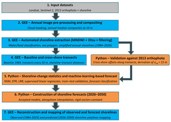
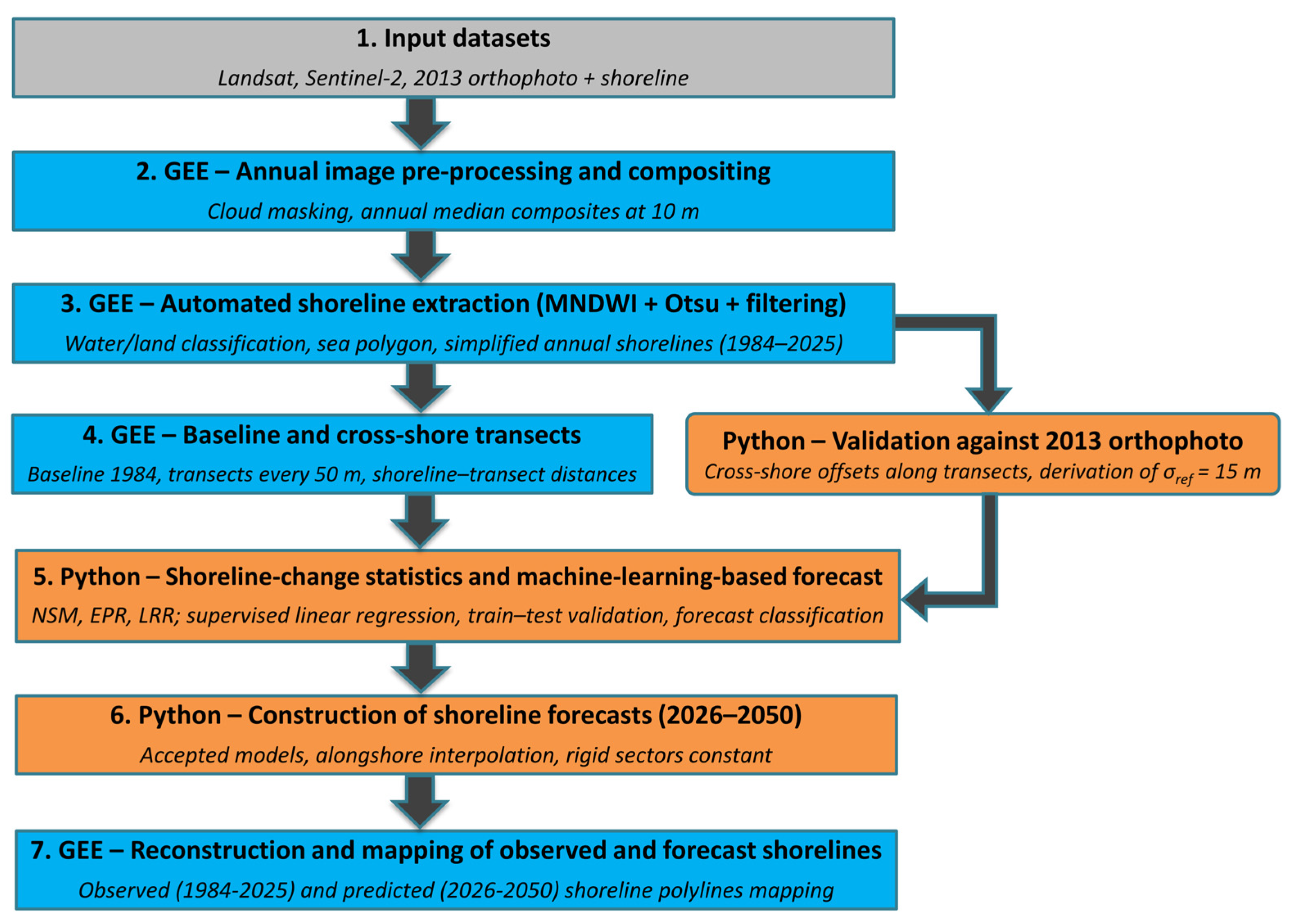
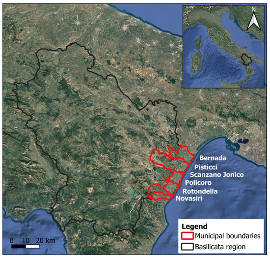
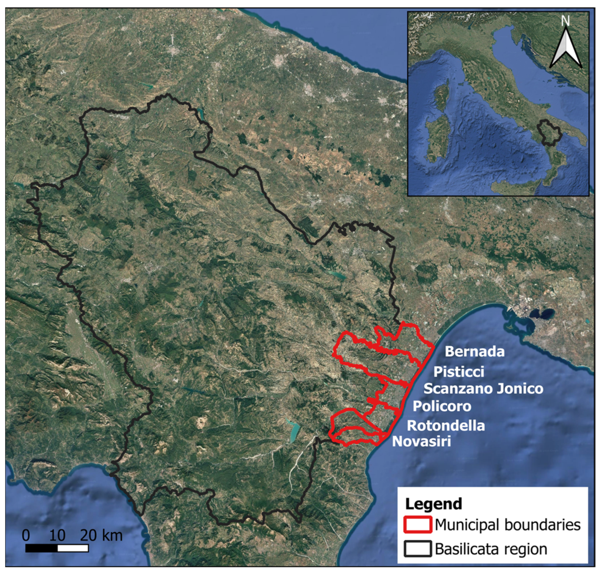
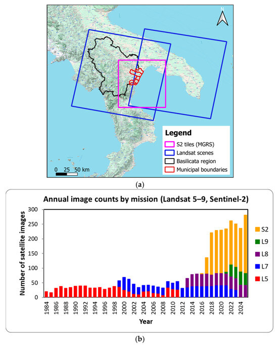
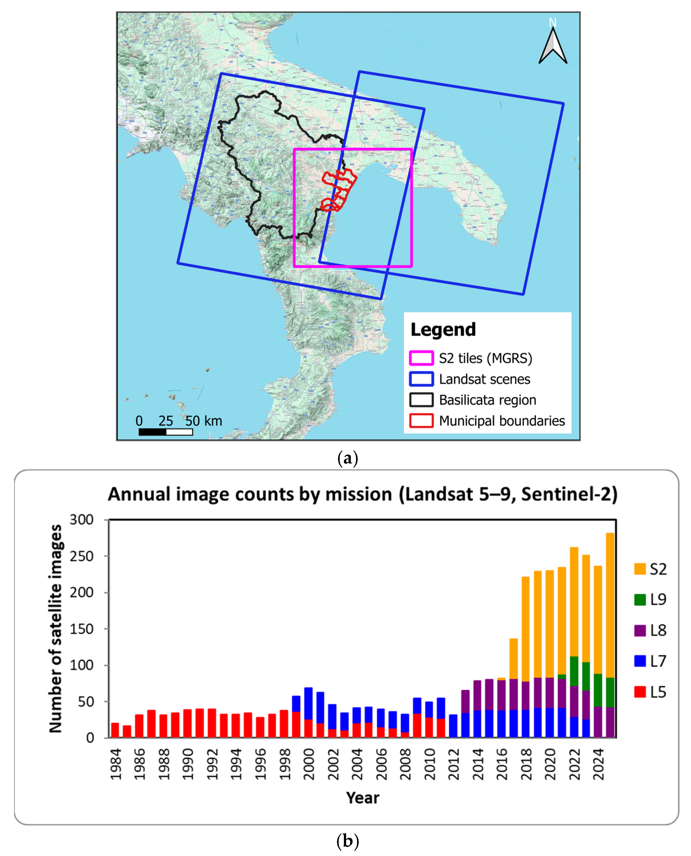
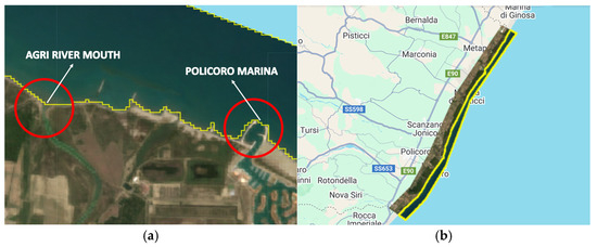
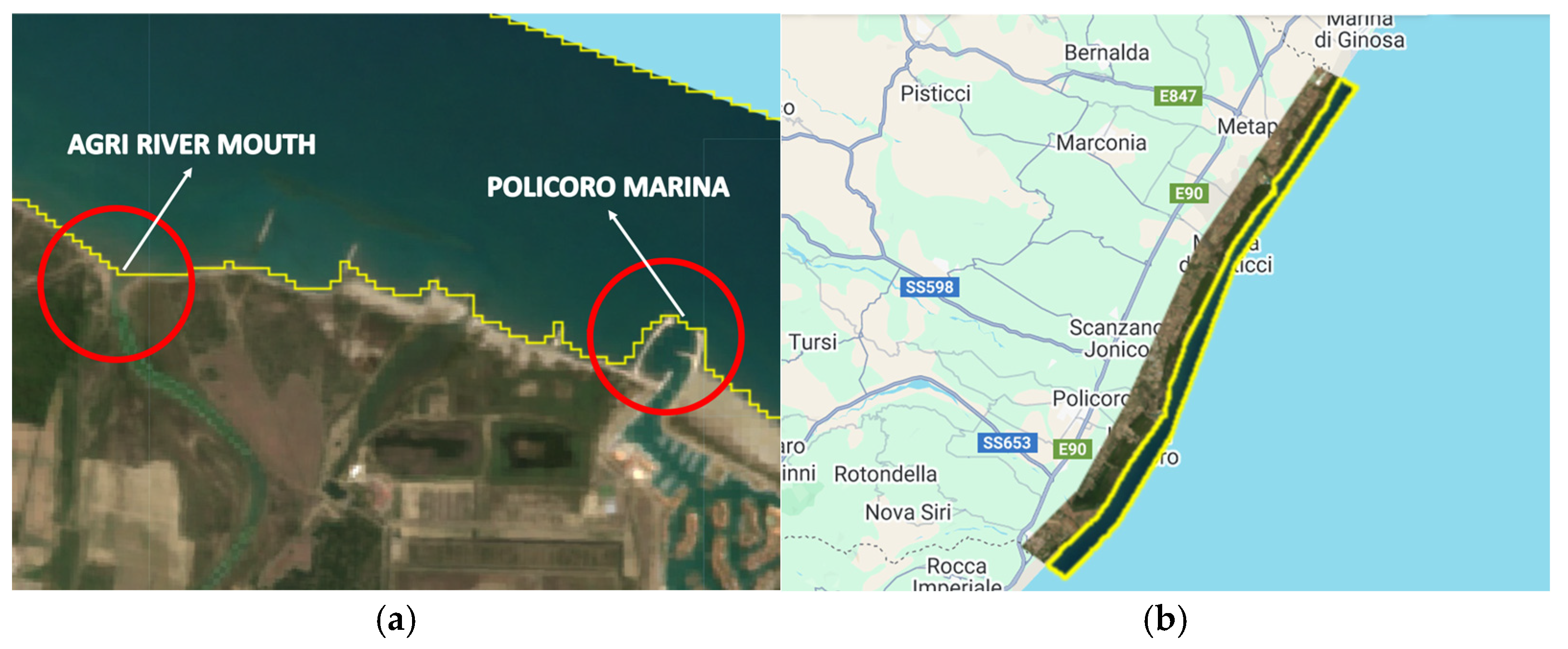
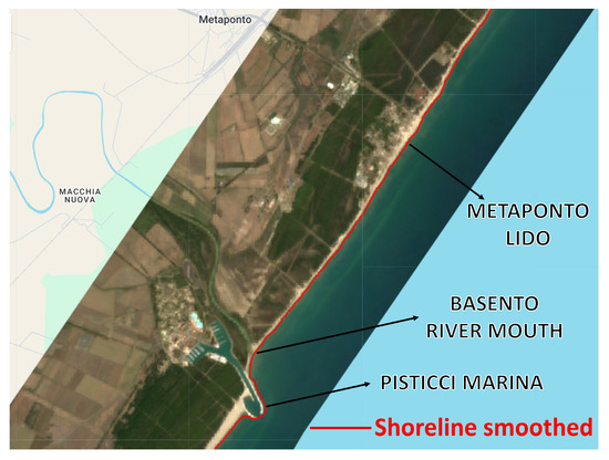
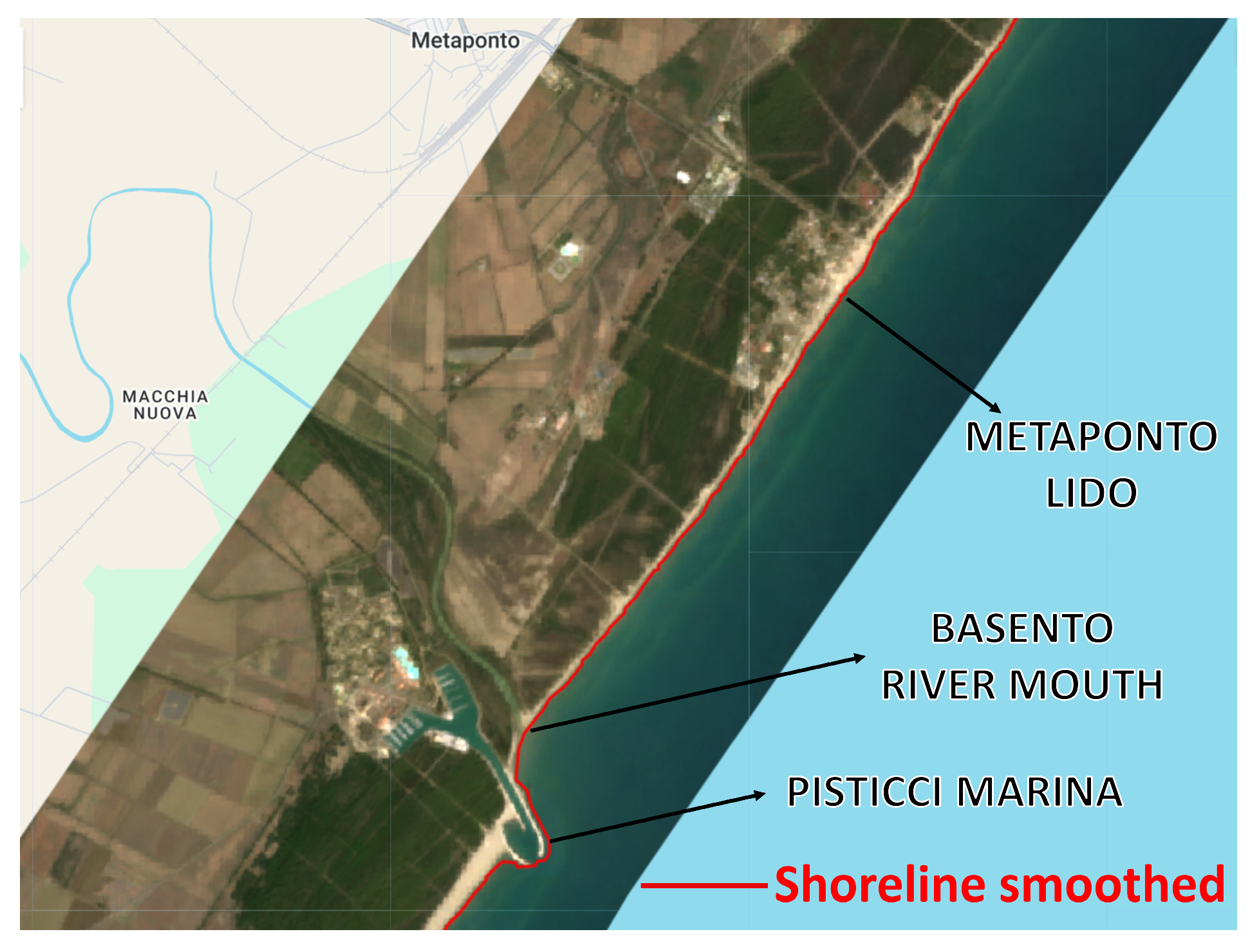
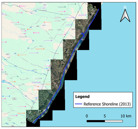
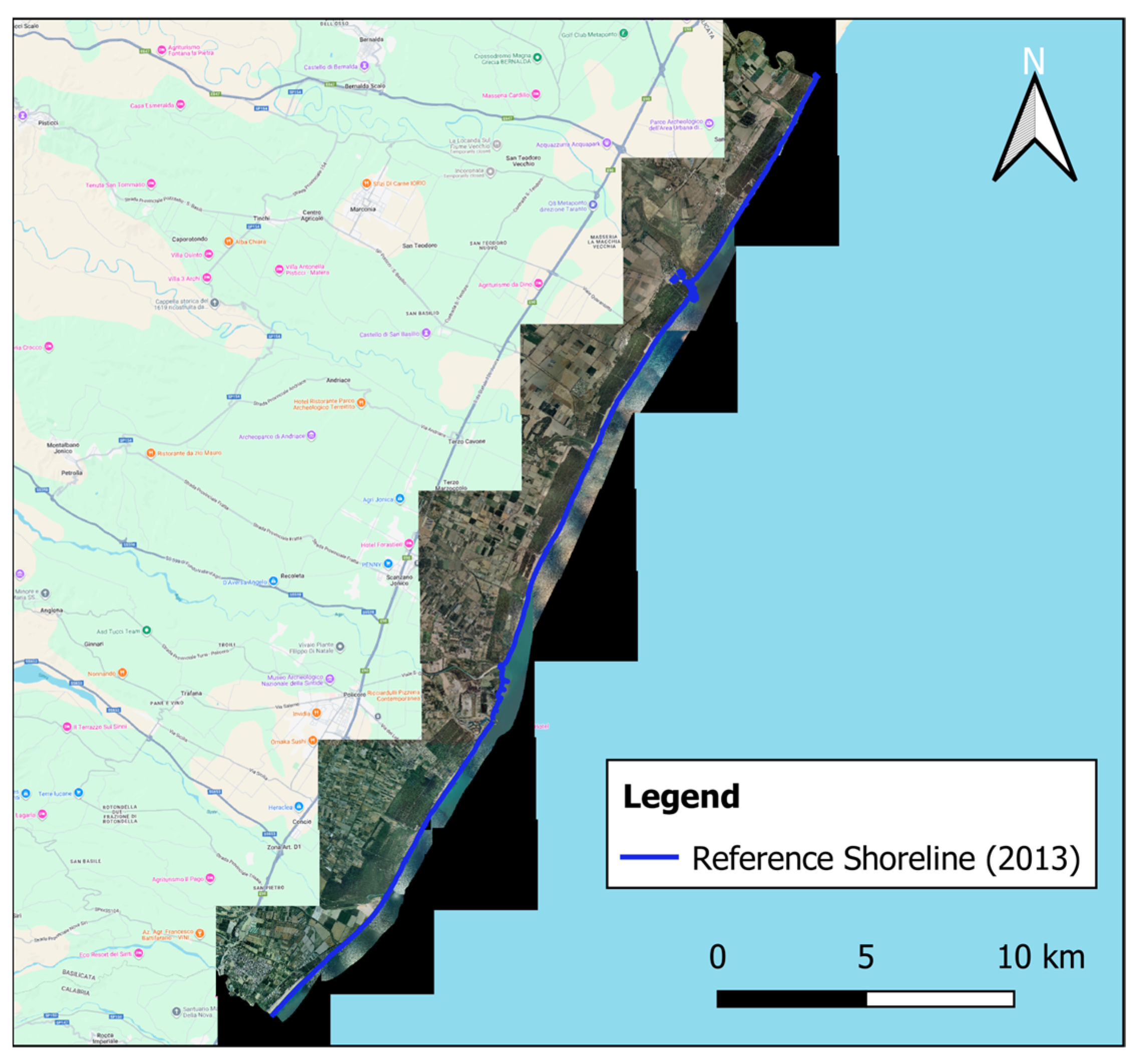
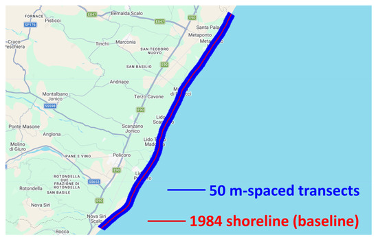
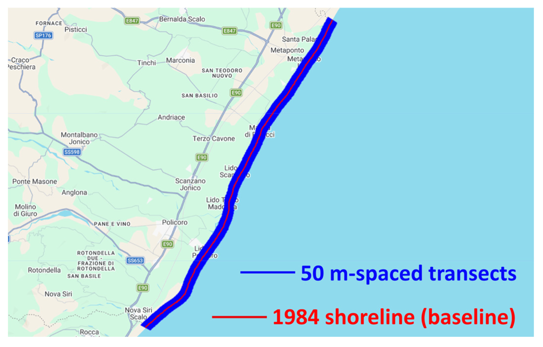
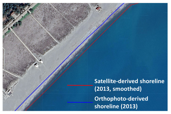
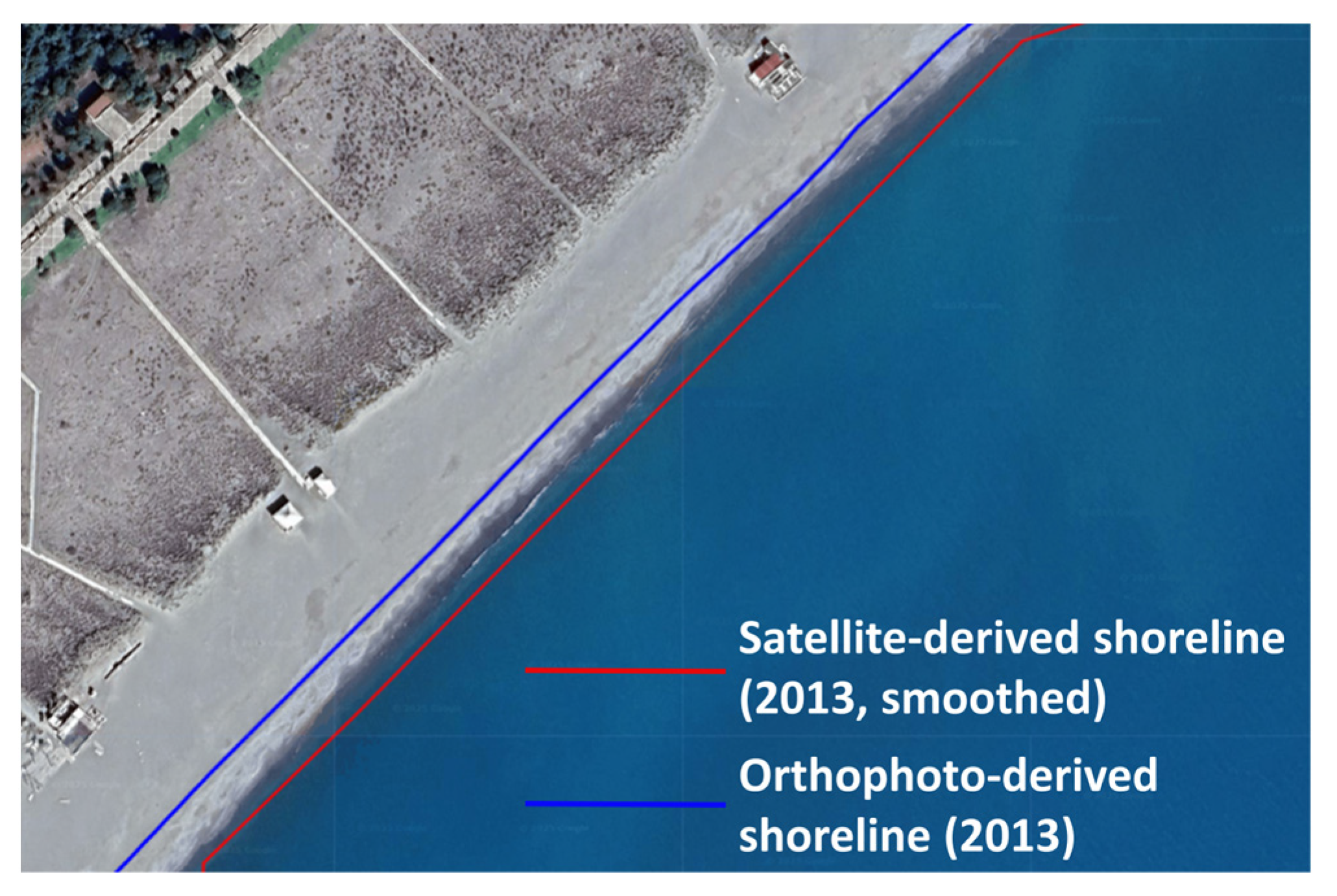
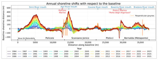
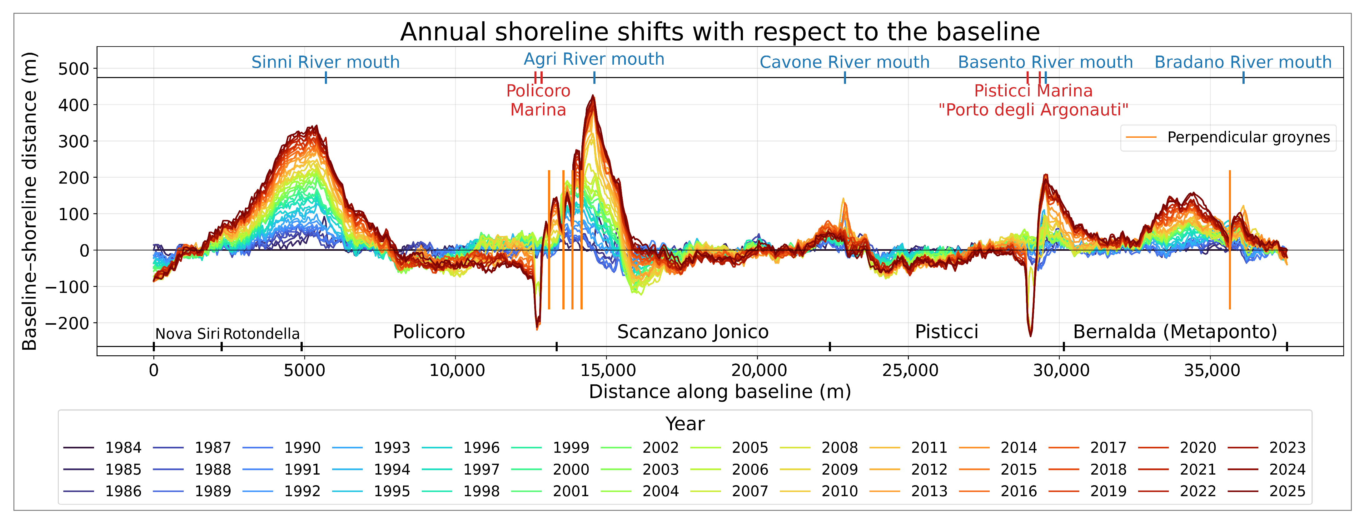
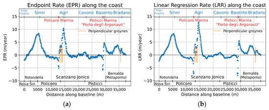
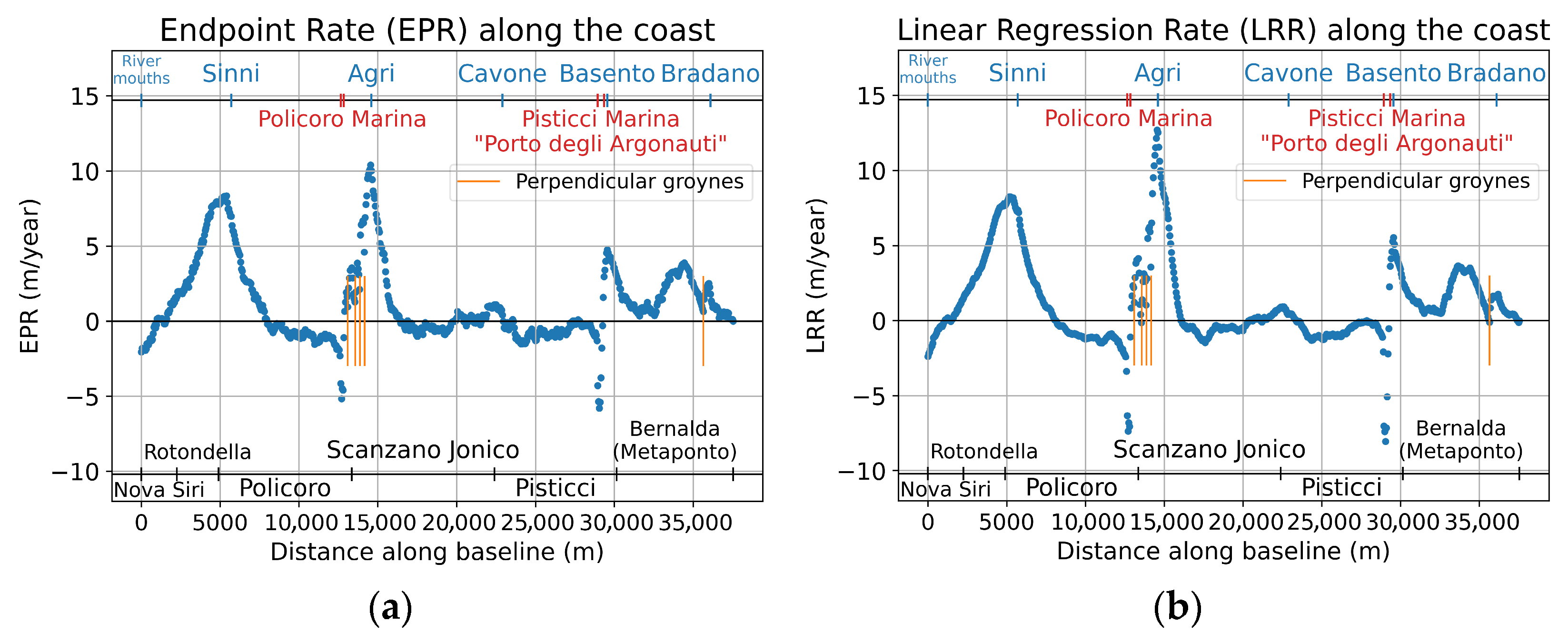
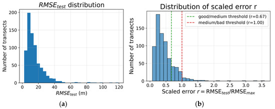
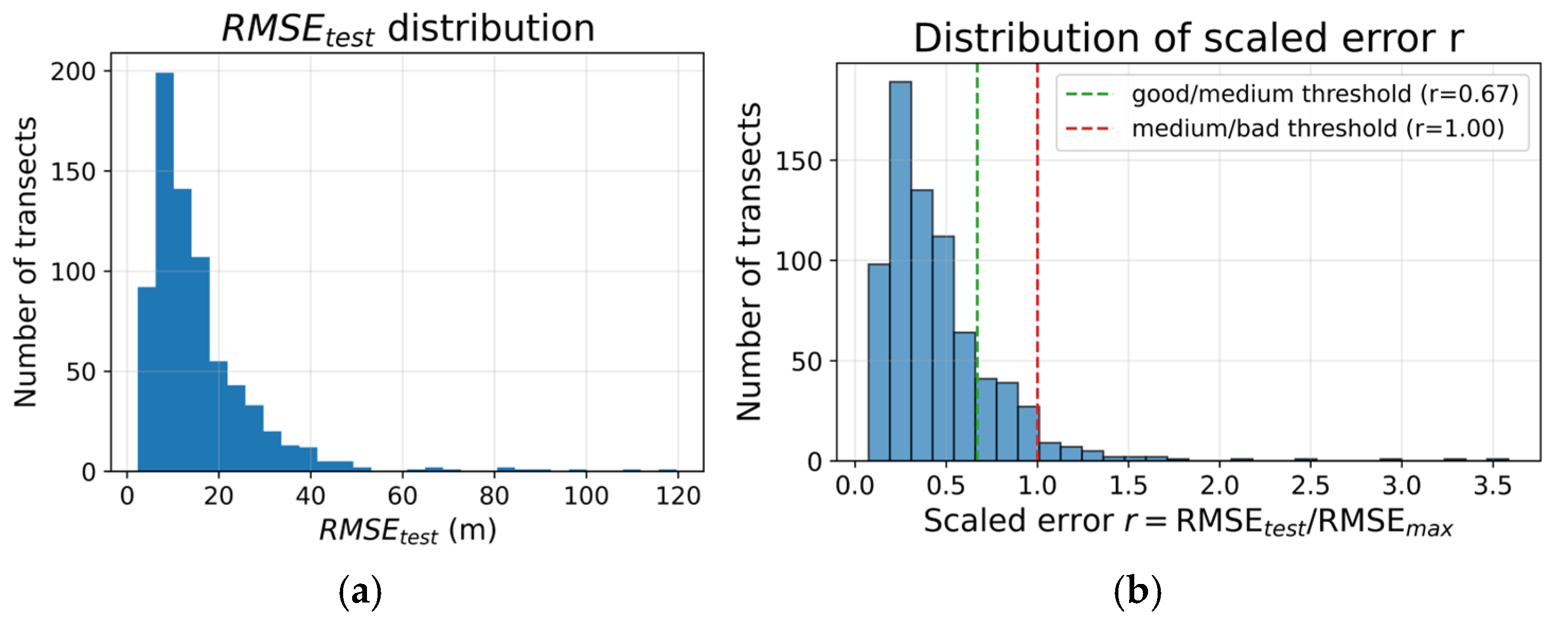
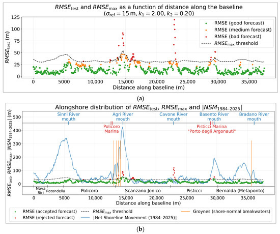
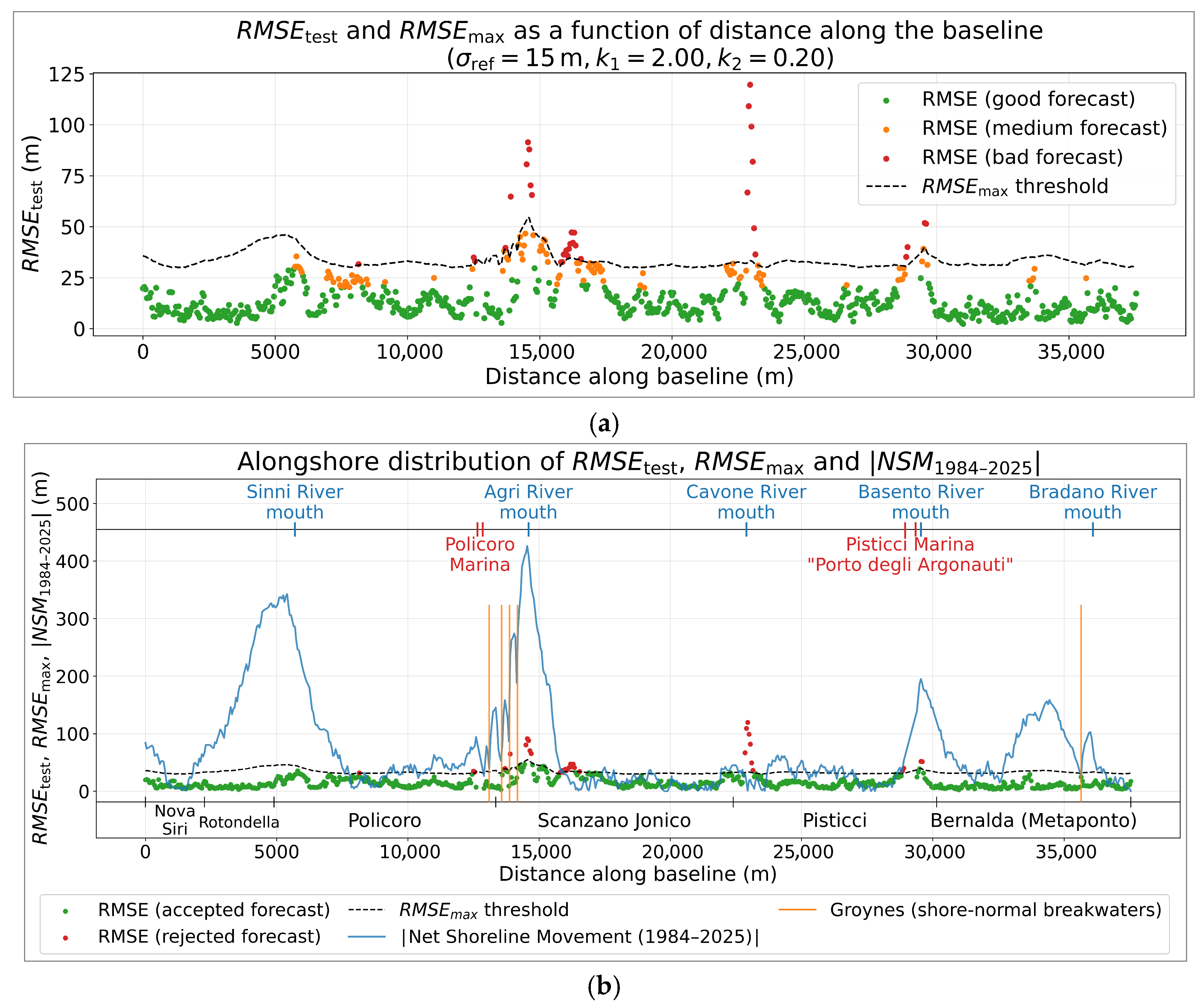
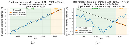
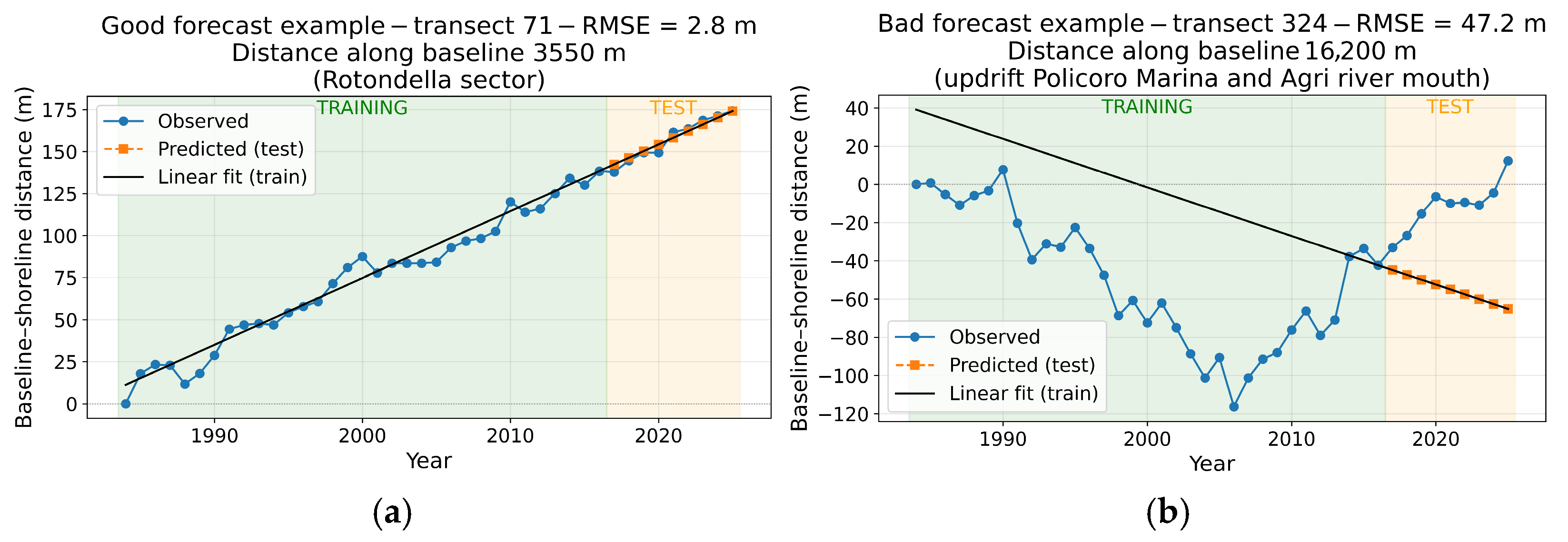
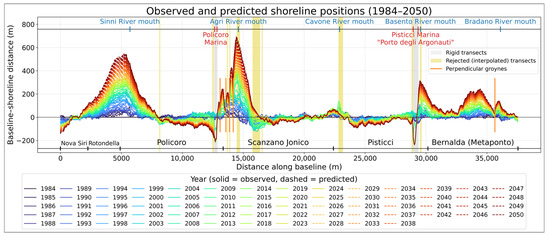
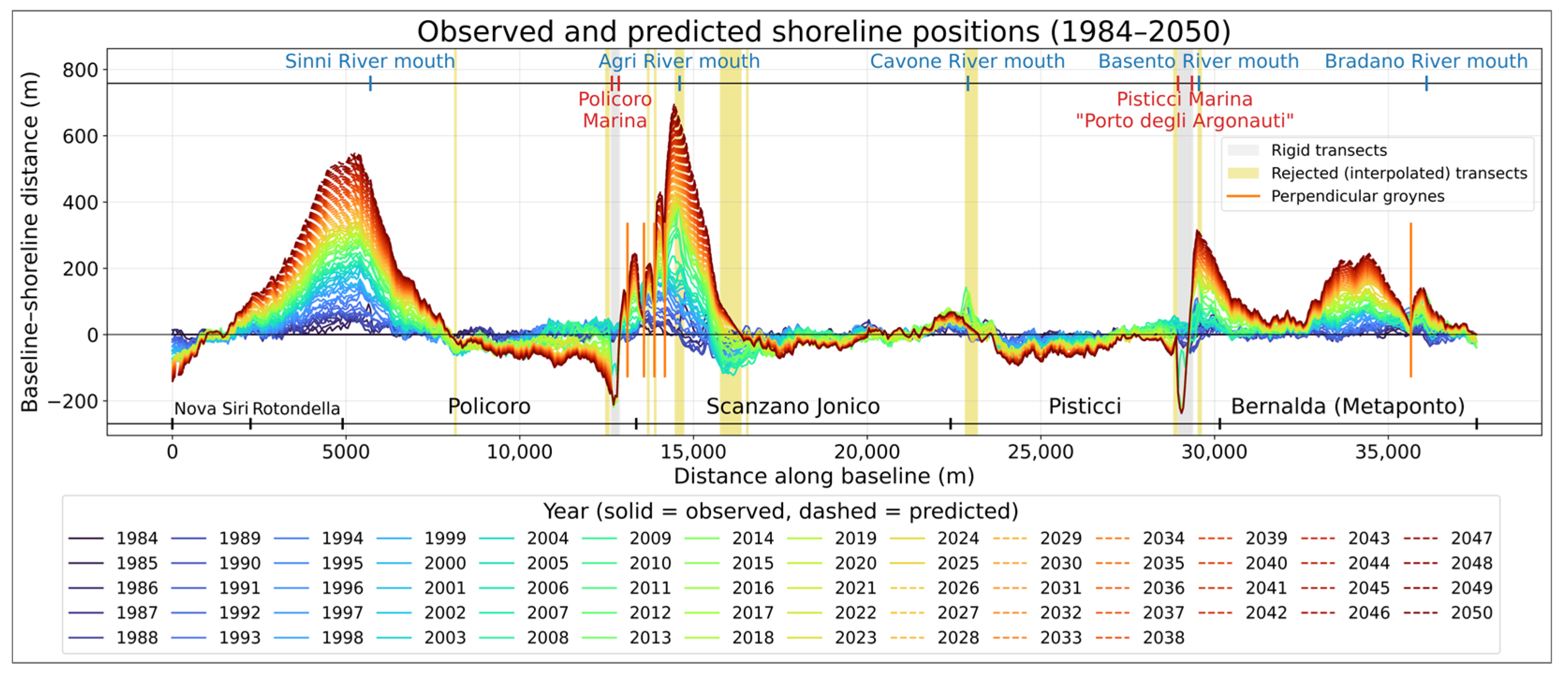
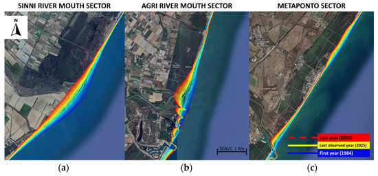
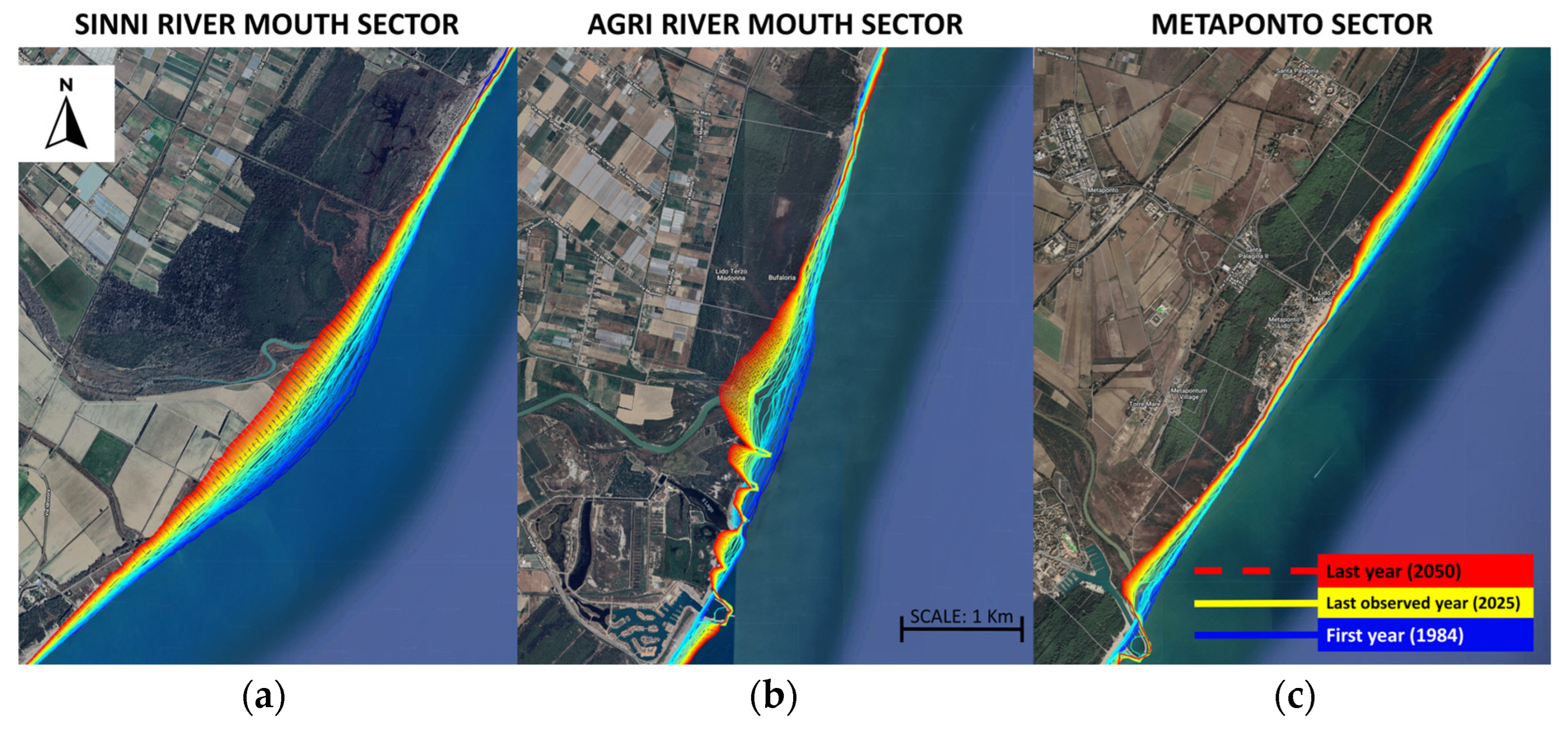

Disclaimer/Publisher’s Note: The statements, opinions and data contained in all publications are solely those of the individual author(s) and contributor(s) and not of MDPI and/or the editor(s). MDPI and/or the editor(s) disclaim responsibility for any injury to people or property resulting from any ideas, methods, instructions or products referred to in the content. |
© 2026 by the authors. Licensee MDPI, Basel, Switzerland. This article is an open access article distributed under the terms and conditions of the Creative Commons Attribution (CC BY) license.