Article

Understanding Spatial Autocorrelation: An Everyday Metaphor and Additional New Interpretations

by
Daniel A. Griffith
School of Economic, Political and Policy Sciences, University of Texas at Dallas, 800 W. Campbell Road, Richardson, TX 75080, USA
Geographies 2023, 3(3), 543-562; https://doi.org/10.3390/geographies3030028
Submission received: 22 June 2023 / Revised: 11 August 2023 / Accepted: 22 August 2023 / Published: 27 August 2023
(This article belongs to the Special Issue Mapping of People and Places for Statistics)

Abstract

:
An enumeration of spatial autocorrelation’s (SA’s) polyvalent forms occurred nearly three decades ago. Attempts to conceive and disseminate a clearer explanation of it employ metaphors seeking to better relate SA to a student’s or spatial scientist’s personal knowledge databank. However, not one of these uses the jigsaw puzzle metaphor appearing in this paper, which exploits an analogy between concrete visual content organization and abstract map patterns of attributes. It not only makes SA easier to understand, which furnishes a useful pedagogic tool for teaching novices and others about it, but also discloses that many georeferenced data should contain a positive–negative SA mixture. Empirical examples corroborate this mixture’s existence, as well as the tendency for marked positive SA to characterize remotely sensed and moderate (net) positive SA to characterize socio-economic/demographic, georeferenced data.

1. Introduction

Salvati [1] points out that “evidence from the analysis of scientific databanks and repositories indicates how the geography discipline has a strong potential for growth and [facilitating] the dissemination of complex global problems.” Realizing this potential requires a wider awareness and deeper understanding of an often glossed over, ignored, or unschooled fundamental property of all of the geospatial data housed in the databanks and repositories he mentions, namely, spatial autocorrelation (SA)—the tendency for (dis)similar attribute values to cluster on a map. As Griffith [2] professes, SA is everywhere! Accordingly, it is an essential ingredient for “develop[ing] and offer[ing] new strategies, visions and proposals on the role of sustainability and resilience related to urban and rural contexts” [1], such as partially constituting the spatial statistical theory underlying tessellated stratified random sampling necessary for economically and efficiently monitoring and “studying [the] degree of resilience and future (sustainable) development [of large territories]” [1]. Not only is SA a fundamental property of georeferenced data, but it also is a fundamental geographic concept (e.g., Tobler’s [3] First Law of Geography; see https://www.researchgate.net/publication/276917830_Concepts_and_Principles_for_Spatial_Literacy (accessed on 24 August 2023)). Its history dates back to its informal, tacit, non-verbal awareness concept formation recognition by, for example, Spilsbury in 1767 [4], who invented the jigsaw puzzle to teach geography, and Brandes in 1816 [5], who invented the isobar map to visualize general west-to-east movements of low pressure across Europe. Nearly a century later, SA had its formal concept creation recognition by Student [6], followed by a quarter century of acknowledgements about its correlated data source [7,8,9] and its impacts on agricultural experimental designs [10,11], its quantification by Moran [12] and Geary [13], its popularization by Cliff and Ord [14], as well as Journel and Huijbregts [15], and its promotion as part of standard spatial statistical/econometric practice by Paelinck and Klaassen [16], Anselin [17], Cressie [18], and Haining [19], among others.
The concept of SA may be more meticulously defined as follows:
Coupling a tertile-classified set of attribute values [i.e., relatively high (H), intermediate (M), and relatively low (L) magnitude groups] with a posited geographic neighbors definition (e.g., nearby points, adjacent line segments, and/or juxtaposed polygons sharing a non-zero length common boundary—the rook designation, based upon its resemblance to chess piece moves), the tendency for pairs of H, of M, and/or of L values (positive SA), or the tendency for contrasting high-low (H-L) or low-high (L-H) value pairings as well as still pairs of M values (negative SA), to be neighbors as defined by this given geographic-based construction.
This tertile definition builds upon Anselin’s [20] local SA index conceptualization, which translates points in a Moran scatterplot into neighboring pairings denoted by high-high (H-H), low-low (L-L), H-L, and L-H; insignificant areal units constitute the M values. SA has other correlated data parallels, including those involving matched pairs, time series, space-time series, and network series [21].
During its catapulting into the forefront of the quantitative spatial sciences, many students, in particular, of quantitative geography found understanding SA and its consequences a challenge, spawning a set of earlier publications devoted to explicating it [22,23]; Griffith also published a monograph with this title in 1987). Contemporary literature, including Getis [24], Goodchild [25], Griffith [26], Haining [27], Legendre [28], and McMillan [29], contains a number of standalone explanatory treatments of SA. Today, the body of literature dedicated to SA is sizeable (Figure 1; for an updated version, see [30]). The objective of this paper is to augment this body of literature by explaining the concept of SA utilizing a common everyday object as a metaphor. Doing so contributes to knowledge particularly by establishing a better comprehension of negative SA, one of the most neglected concepts in spatial statistics/econometrics [31], as well as mixtures of positive and negative SA [32,33].

1.1. SA: An Important Geospatial Synoptic Statistic

Elementary descriptive statistics are important for quantitative analyses because they condense a numerical dataset’s information content into a few informative summary values about those data. Two vital descriptors are the mean and the variance because they respectively reveal a typical value and the spread of a dataset, even if the mean is a function of other variables when treated in a multivariate context. SA becomes a third crucial descriptor for georeferenced data—Goodchild [25] describes it as being endemic—because, in part, it exposes the presence of inflation in the variance, and, in part, because it represents redundant information that supplies the “essential economies that allow complex surfaces to be represented in manageable volumes” [25].
Couching this SA notion within a more technical statistical context, Legendre [28] emphasizes the commonly cited undermining by SA of the standard statistical analysis independent observations assumption, mentioning that it most often materializes in a geographic distribution as patches or gradients. Haining [27] highlights this SA non-independence feature as being instrumental to geography’s contribution to spatial statistics, commenting that SA relates to both scale and resolution of geographic data. Cliff and Ord [14] acknowledge that mis-specified regression models can create spurious residual SA, a theme discussed in detail by McMillen [29], and in terms of omitted variable beckoning by Griffith and Chun [34], can introduce omitted variable bias, especially in the presence of disregarded negative SA [33]. In these two latter multivariate contexts, a response variable’s mean varies, rather than being a constant (e.g., only an intercept term); SA contained in a response variable is a function of either that latent in related covariates, or spatial lag terms appearing in spatial autoregressive model specifications (e.g., conditional autoregressive (CAR), simultaneous autoregressive (SAR), and autoregressive response (AR) versions being the most popular) that attempt to usurp missing variable effects. Meanwhile, Goodchild [25] echoes the sentiment of the preceding paragraph, noting that SA is “… a monotonically decreasing function of distance [and hence] a fortunate characteristic of a wide range of spatially distributed phenomena.”

1.2. SA and Geographic Scale/Resolution

Legendre [28] addresses the geographic scale (i.e., geographic landscape size, relating to increasing domain sampling designs) issue, arguing that SA-related global patterns across a geographic landscape materializing as gradients arise from spatial (e.g., distance decay) processes or wide-ranging underlying common factors that elicit the formation of comparable outcomes in different regions and locations. Likewise, SA-related local patterns, which, landscape-wide, appear as disjoint patches separated by interstices, elicit the formation of numerous geographically small concentrations of outcomes at dispersed locations. Geographic scale provides the perspective that casts a clustering of similar values as being a gradient or patchiness. Pawley and McArdle [35] partner this scale issue with a recognition that the target of inference helps determine when SA presents data analysis complications or an opportunity to achieve additional effectiveness and/or robustness.
The geographic resolution (i.e., size of an areal unit polygon, relating to infill spatial sampling designs) issue involves some sort of data averaging within polygons: as polygons increase in size, more geographic averaging occurs, which has an accuracy highly correlated with any latent degree of positive SA. This averaging implies that, in practice, the SA measurements should change as resolution becomes coarser. Employing regular square quadrats, Chou [36] finds that SA measures increase in magnitude as resolution becomes finer, at a logarithmic rate; Zhang et al. [37] essentially corroborate this finding. Rodrigues and Tenedorio [38] report that the shape of irregular areal unit polygons also impacts SA measures, with aggregation of such nonuniform shapes varying in size not necessarily strictly rendering decreasing values with increasing coarseness. Di et al. [39] also detect an inverse relationship between resolution and SA measurement, while uncovering a tendency for SA quantifications to decrease in magnitude when irregular replace regular square shaped areal unit polygons. Describing this situation as the resolution sensitivity of SA, Mohan et al. [40] show that the aforementioned negative relationship is not necessarily a monotonically decreasing function—a finding similar to that by Rodrigues and Tenedorio [38]—devising a resolution correlogram tool based upon popular SA indices to adjust for this sensitivity.
The principal implication here for the metaphor explicated in this paper is that the sizes, shapes, and numbers of jigsaw puzzle pieces [41] affect the interface between a puzzle and SA addressed in the ensuing discussion. It also alludes to the issue of geographic scale and resolution. If a puzzle’s size is held constant, then increasing its number of pieces (all of which frequently are alike in total area) is equivalent to changing its geographic resolution. As geographic resolution increases, visual clues from puzzle pieces become more obscure; as geographic resolution decreases, clues from border buffer areas becomes more informative. Although artwork, piece size/shape, and color range can contribute to the degree of difficulty for solving a given puzzle, its number of pieces tends to be most strongly directly correlated with its degree of difficulty. As noted in the preceding paragraph, SA exhibits a similar type of tendency: it tends to increase in magnitude as resolution becomes finer, at a logarithmic rate.

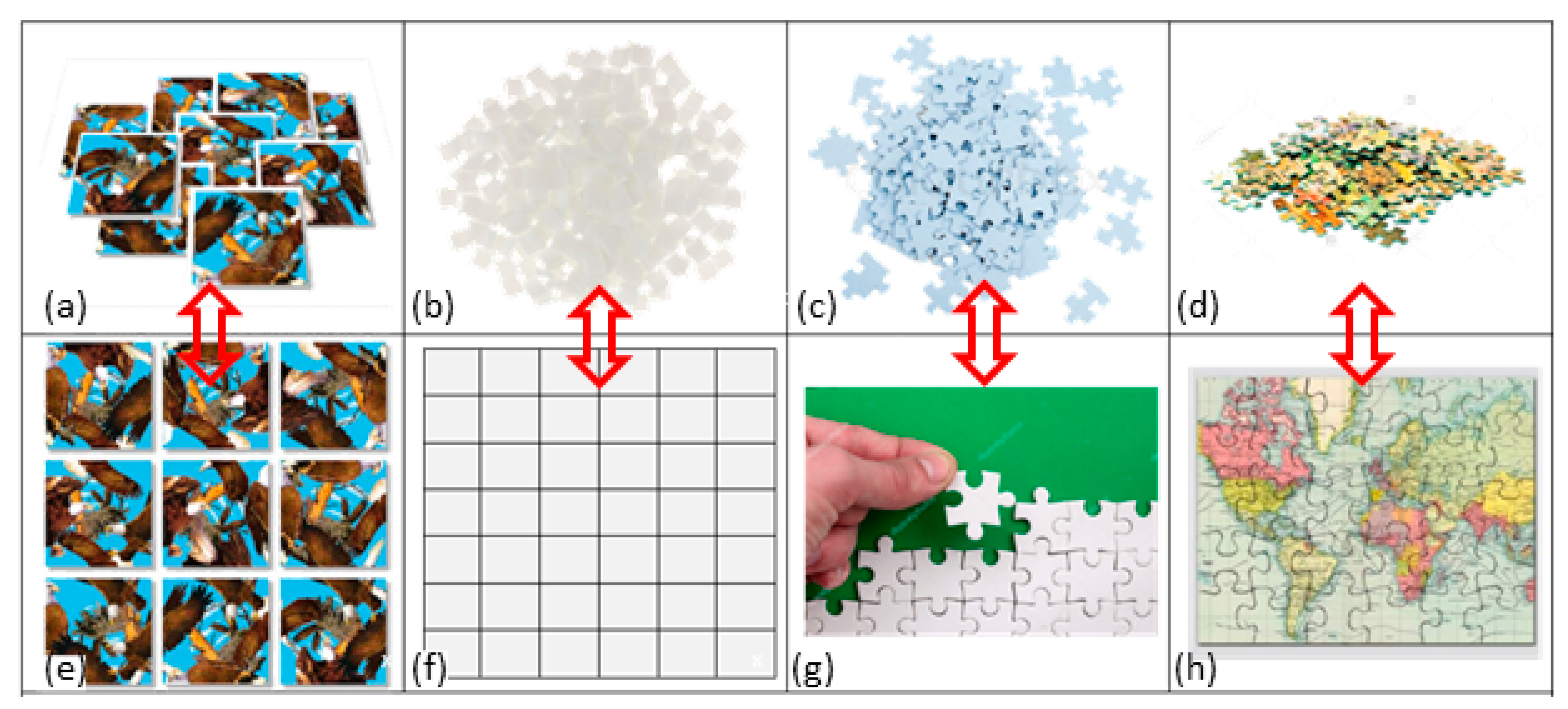
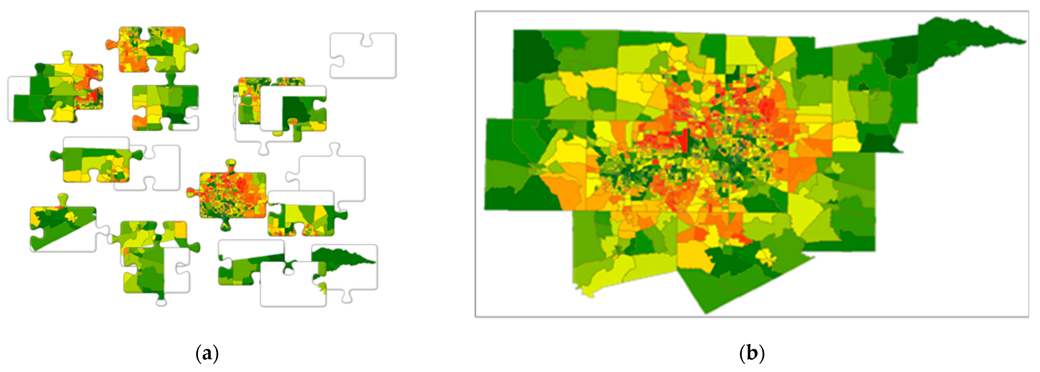
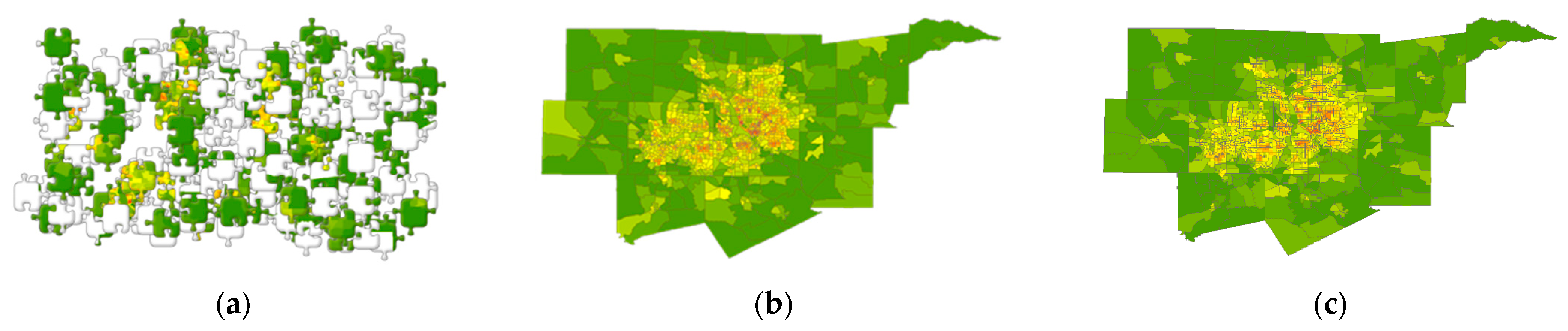
2. The Jigsaw Puzzle: An Everyday Object Metaphor

In the mid-1700s, Londoner John Spilsbury, a cartographer among other professions, drew a map of the world on the top of a piece of wood, and then used a fretsaw/saber-saw tool to cut it into its constituent countries, in order to craft an educational tool [4]: this was the invention of the jigsaw puzzle. Such a puzzle may be defined as a dissected tiling of mutually exclusive and collectively exhaustive often weirdly shaped small pieces (tiles originally cut by a fretsaw machine) coupled with a challenge of reconstructing the initial tiling by fitting these pieces together to assemble the original complete image or form the original complete shape. Most jigsaw puzzles comprise interlocking small pieces; the dissection imposed upon some of these puzzles involves a regular, whereas for others it involves an irregular, tessellation. Noteworthy characteristics of the pieces include: tabs, which take area away from, and cut out slots, which forfeit area to, adjacent pieces; whether or not pieces are fully interlocking (adjacent pieces connect with tabs/slots such that horizontally/vertically moving one piece results in moving an entire cluster of pieces, preserving their structural and visual connections); and, similarity of piece shapes (e.g., single/uniform shaped pieces have tabs protruding on opposite sides, with corresponding slots cut into the intervening sides). From shortly after their invention through to today, jigsaw puzzles are notoriously popular around the world, furnishing an ideal metaphor for raising the awareness of SA being everywhere.
Given the jigsaw puzzle’s cartographic roots, one of its especially appropriate features is its relationship to SA (re. Tobler’s First Law of Geography). Analogous to conventional linear correlation, SA is best described with reference to a bivariate statistics scatterplot, which is a two-dimensional (2-D) graph portraying plotted paired values for two variables, X and Y, with reference to its axes (which may be expressed as z-scores; i.e., zi = y i y ¯ s Y for areal unit i, where y ¯ and sy respectively denote the arithmetic mean and standard deviation of elementary statistics). However, portraying SA rather than a standard bivariate correlation scatterplot replaces X with zi for the horizontal axis, and, for the vertical axis, Y with the sum of neighboring zi values (i.e., using algebraic notation, j = 1 n c ij z j , where cij = 1 when areal units i and j are, and 0 when they are not, neighbors, perhaps employing the rook adjacency definition). This modified statistical graphic is the Moran scatterplot, whose trend line is proportional to a dataset’s Moran Coefficient (MC; this covariation-based index, arguably the most popular SA quantifier, resembles the Pearson product moment correlation coefficient)—the scaling constant is n divided by the sum of the entries (e.g., 0 s and 1 s) in the attached spatial weights matrix (SWM; which is like an Excel spreadsheet whose row and column labels are the same sequence of areal unit polygons/locations, and whose cell entries are 1 if row and column areal units are neighbors, and 0 otherwise; this tabular data quantifies the topological arrangement of areal units forming a map) indicating which areal units are neighbors. The pattern of the resulting cloud of points, as well as the trend line, reveals the nature and degree of any SA present (see Figure 2). Figure 2 portrays the SA latent in jigsaw puzzles depicted by Figure 3b–d.

3. What Is SA? Illustrative SA Jigsaw Puzzle Cases

Figure 3b,c exemplify the two essential components for solving a jigsaw puzzle, a measure of jigsaw piece physical compatibility for adjoining a pair of pieces (re. congruent shape characteristics, with prominent ones relating to spatial competition notions; in other words, negative SA facets), and puzzle assembly visual coordination strategy (re. image continuity across puzzle pieces, with prominent ones relating to spatial synchronization forming visible map patterns; in other words, positive SA facets). Solving a jigsaw puzzle often requires analysis of mixtures of shape compatibilities (i.e., fitting the appropriate tabs, which take away area from a neighboring piece, into their corresponding slots, which represent forfeited area to a neighboring piece) and image coherency; in other words, recognizing positive and negative SA mixtures. This recognition supplements that provided through the decomposition of SA by quadrant in a Moran scatterplot.

3.1. A Case of Zero SA

Figure 4b,f furnish an example of zero SA. The puzzle solution is a rectangular region layout composed of P-by-Q (i.e., horizontal-by-vertical) regular square pieces, all of the same color and shape differentiable at best solely by visibly imperceptible trace random variations of a single color (e.g., grey). Combinatorial theory [43] states that this jigsaw puzzle has at most n! (n = PQ square pieces) possible solutions (i.e., P-by-Q arrangements of the n tile puzzle pieces) for the rectangular region layout alone, all of which here reconstruct exactly the same blank image (hence, n! repeated arrangements, yielding (n!)/(n!) = 1 solution; e.g., see https://www.get-digital-help.com/permutations-with-and-without-repetition/ (accessed on 23 August 2023)); many other non-rectangular polyomino puzzle layouts also are conceivable (e.g., a linear arrangement or rectangular frame/outline of tiles, assortments similar to formations such as those visible in the Tetris video game), with each having only one solution regardless of individual puzzle piece placements. All puzzle pieces are both the same shape and the same color; therefore, neither pattern (i.e., positive SA) nor individual piece shapes (i.e., negative SA) exists to supply assembly clues; this puzzle does not have a unique constructable image outcome.
Rather than the previously mentioned regular polygon shaped (e.g., triangle, square, hexagon) blank puzzle pieces, such same-shaped pieces might reconstruct a random patterned abstract art image (e.g., selected Janet Sobel or Jackson Pollock drip paintings), which is extremely difficult to solve even with irregular polygon shapes. The SA for its uniformly shaped and dimensioned pieces version failing to render a 2-D patterned image would be near zero.

The 0/0 Conundrum

The Figure 4a,f blank square tiles behave like a constant numerical value, say c, geographically distributed across a map, that when plugged into SA indices—which are ratios having either covariations or squared paired comparisons in their numerators, and variance in their denominators—yield zero divided by zero (0/0). This division is an invalid mathematical operation (i.e., its outcome is undefined and/or indeterminant), violating the fundamental properties and rules of ordinary arithmetic: 0/c = 0 and c/c = 1, if c ≠ 0. However, when c = 0, mathematicians and scientists may assign different context-dependent values (i.e., 0 or 1) or interpretations to its result—limits in calculus (e.g., the extended real number line a la L’Hospital’s rule), or other mathematical concepts (e.g., the projected extended real number line so that division by zero equals ∞)—depending upon their situation (i.e., conceptualizations and/or needs).
The SA covariation index employs a doubly centered SWM. A rescaling of its eigenvalues—n quantities from linear algebra theory characterizing matrices—computes this index. One of these eigenvalues is guaranteed to be zero, with an accompanying eigenvector proportional to the vector 1. In other words, this neighboring value’s covariation standpoint invents a situation in which the definition of 0/0 implies zero SA; L’Hospital’s rule asymptotically endorses this view. The intuition here is that no arrangement of loose blank regular square tile jigsaw puzzle pieces has observational correlation; any tile can be placed anywhere when completing a puzzle. Meanwhile, the squared paired comparisons index employs the Laplacian SWM version. Copycatting the covariation formula, a rescaling of its eigenvalues delivers its index values. As before, one of these eigenvalues is always zero, with an accompanying eigenvector proportional to the vector 1. In other words, this squared paired comparison of neighboring values stance contrives a situation in which the definition of 0/0 implies perfect positive SA; the calculus quotient limit theorem endorses this view. The intuition here is that after organizing a set of loose blank regular square tile jigsaw puzzle pieces into an arrangement with locational tagging, knowing the tile blankness at any particular location in this configuration automatically bestows knowing blankness anywhere else in it. In contrast, L’Hopsital’s rule renders near-zero SA only for typical neighborhood structures, an inconsistency attributable to some of the GR’s weaknesses. Nevertheless, both cases are technically singular, necessitating conceptual instead of computational reasoning for their clarifications.
Therefore, because the metaphor in this paper addresses clues for constructing jigsaw puzzles, it gives preference to the former of these two contextual interpretations of 0/0: a pile of blank puzzle pieces denotes zero SA.

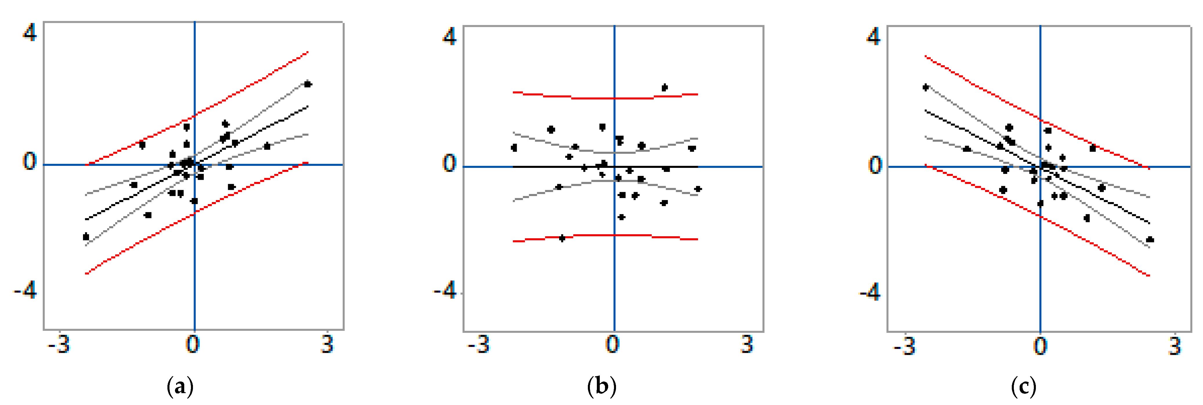
3.2. A Case of Pure Positive SA

The preceding zero-SA example emphasizes that positive SA relates to global, reginal, and local patterns in an image formed by a jigsaw puzzle, regardless of the shape of the pieces into which a jigsaw puzzle dissects/partitions an image. Figure 4a,e furnish an example of pure positive SA. The jigsaw puzzle solution does not depend upon shapes of pieces; all pieces are square tiles of the same size. Rather, it depends upon only matching patterns especially along the borders of pieces. Synchronization is the solution key. A unique solution exists, although one could argue that at least four orientation-free identical solutions exist (rotating the completed puzzle 0°, 90°, 180°, and 270°). Computational algorithms for solving jigsaw puzzles exploit this image continuity property [44]; Guerroui and Séridi [45] supply a brief computer science history of these solutions.

3.3. A Case of Pure Negative SA

If a puzzle’s outline is rectangular and the number of its pieces is known, then shape recognition can establish the four corners, all of the edge, and the set of center pieces; a circular outline removes only the corner pieces identification. Consequently, such a puzzle can be (nearly) solved by entirely ignoring its image—because its pieces could be put together into the same configuration as solving this puzzle utilizing its image—and initially placing all of its pieces facing down (revealing blank pieces); of course, within this context, piece shape replications promote possible final image errors. As Figure 3c highlights, the tabs and slots of pieces relate to negative SA. Figure 4c,g furnish an example of this SA nature. The only information available is polygon shapes. Adjacent pieces annex area with their tabs, and forfeit area with their slots; these processes are a spatial competition trademark. If the irregular pieces of a puzzle are unique, then its solution is unique. As the number of duplicate shaped pieces increases, the number of positions identical shapes can match increases, and, thus, the number of non-unique solutions increases, requiring positive SA clues to obtain a unique solution. Computational algorithms for solving jigsaw puzzles exploit this shape compatibility property, too.
Avoiding erroneously inferring that negative SA solely relates to polygon shape requires a closer examination of the word metaphor’s definition: a rhetorical account figuratively, rather than literally, comparing two unrelated entities by highlighting their similarities to convey a better understanding of the more complex of the two through simplifying analogy in a vivid, imaginative, and expressive manner. This is the situation for negative SA and the jigsaw puzzle, which casts it in physical terms: spatial competition manifests itself via annexing and forfeiting adjacent polygon area. However, this instrument also symbolizes fantasizing the confiscating and relinquishing of phenomena housed in areal unit polygons or locations in a way that is reminiscent of economist Adam Smith’s fictitious “invisible hand in the marketplace” (see Figure 5): unseen hands reach out from areal units to confiscate (i.e., imaginary tabs), with the penetrated units relinquishing (i.e., imaginary slots), attribute quantities, changing the global geographic distribution of interest rather than individual polygon shapes. Mobility and transportation are real-world colleagues of these invisible hands. This is the premise underlying, for example, the provision of a designated bundle of goods/services at a particular central place hierarchy level. The materializing hexagonal checkerboard mosaic (Figure 5c) is an outcome of spatial competition, but in equilibrium and arising from invisible hands pulling a third of the uniformly distributed customer demand from each surrounding lower-level hexagon, with the resultant partially alternating global pattern reducing the maximum possible negative SA toward −0.5. Eaton and Lipsey [46], paralleling a physical simulation experiment outlined and apparently executed by Bunge [47], demonstrate that such equilibria most likely are hexagonal, or potentially square, checkerboard formations. Furthermore, Perrouxian growth pole theory declares that core areas compel their economic agglomeration, commandeering economic growth from their hinterlands, once more producing a checkerboard pattern without tangibly altering geometric outlines of areal units. Agricultural and urban land use location theory also generates negative SA patterns, but ones that tend to focus on geographic margins of production (e.g., transition zones of equal or zero location rent). Nevertheless, the jigsaw puzzle retains its appeal as an enlightening metaphor.

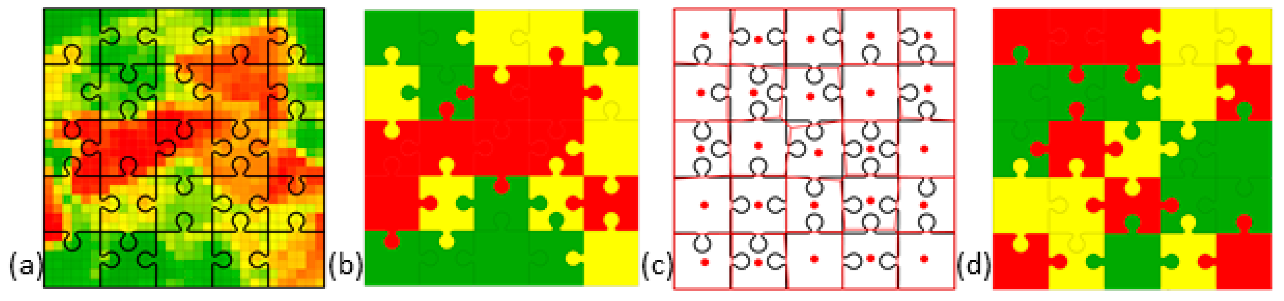
3.4. A Positive–Negative SA Mixture Case

A vast majority of jigsaw puzzles enable both image continuity and shape compatibility of pieces to solve them, meaning replicated shapes do not automatically yield multiple puzzle solutions. In other words, a mixture of positive and negative SA provides clues to guide solutions, as alluded to by Figure 4d,h. Figure 6 furnishes an additional jigsaw puzzle example. Its solution primarily begins with negative SA information (i.e., the four corners and the borders of the region: two rows and two columns of the puzzle). Its completion primarily relies upon positive SA information (i.e., the patterns formed by the internal two-by-three set of pieces), supplemented by some negative SA information (tab/slot conformities). Both steps also utilize the other nature of SA (i.e., pattern continuity and tab/slot compatibility to assemble the correct juxtaposed pieces). In other words, a mixture of positive and negative SA guides the jigsaw puzzle solution, although one or the other nature of SA may regulate a given assembly of local clusters of pieces.

3.5. Some Necessary Remarks about SA

The contemporary history of quantitative geography, geostatistics, and spatial statistics/econometrics reveals that establishing an understanding of SA tracks a rather meandering timeline. This history almost exclusively focuses on positive SA, mentioning negative SA solely for coverage completeness when introducing the topic (and frequently in terms of the two-color pattern on a checkerboard). Established interpretations give many faces to SA. A controversial one essentially relegated to the dustbin of history is SA as a nuisance, a georeferenced data distinction that must be accounted for in a data examination, even though inference about it is not of interest. A mean tends to be the parameter of interest; therefore, this definition can classify most other parameters as nuisances, even the variance. The preceding jigsaw puzzle discussion counters this nuisance assertion, as does the realization that all data have both a geographic location and a time stamp, whether or not they are recorded; relationships between response variables, quantitative analysis findings, and location always merit being of inferential interest, especially when SA constitutes substantive phenomena derivable from conceptual frameworks (e.g., juxtaposed agricultural or urban land uses), and particularly when the goal of a study is prediction (e.g., kriging). An extreme interpretation affiliated with this debatable perspective is that SA is superfluous [48] promotes this argument in the context of showing that SA may fail to impact noticeably upon multivariate statistical research outcomes such as principal components or factor analysis, whereas Diniz-Filho et al. [49] debunk claims that SA is a red herring.
For the most part, the nuisance understanding of SA may be removed from its sundry explanations [26], in part because it is everywhere [2] (e.g., a broadcasted television picture would be unintelligible without SA, an occurrence when static/snow/white noise appears due to the loss of, for example, a cable or terrestrial transmitter signal) with the preceding jigsaw puzzle discussion replacing this specific depiction with that of positive–negative mixtures. SA is everywhere, and more often than not as a simultaneous combination of positive and negative correlation.

4. Materials and Methods: Yet More Faces of SA

Over the years, spatial analysts conveyed an assortment of nuanced SA interpretations [26], a number of which the stated definition in the introduction of this paper reflects in part or in its entirety: self-correlation (e.g., the conversion of a scatterplot into a Moran scatterplot), map pattern (e.g., Figure 3, Figure 4 and Figure 5), redundant information (e.g., Figure 3), a spatial spillover effect (e.g., house prices/valuations), an indicator of areal unit demarcation appropriateness (e.g., the modifiable areal unit problem (MAUP)), a nuisance (see the preceding section), an omitted variables surrogate [34], and a functional misspecification diagnostic tool (i.e., Eire data example in [14,29]). The jigsaw puzzle discussion implies two additional, more focused interpretations: a simultaneous mixture of positive and negative correlated data, commonly a combination in which positive SA dominates; and, the tendency for fine geographic resolution remotely sensed data to display a marked degree of positive SA (e.g., MC ≈ 0.9+), and for coarser geographic resolution socio-economic/demographic data to display a moderate degree of positive SA (e.g., in a preponderance of cases, MC [0.4, 0.6] due to its negative-positive SA mixture)—a wealth of additional evidence reported in the literature, including the aforementioned concerning SA and geographic resolution, supports this latter contention.
In terms of spatial autoregressive methodology, Kao and Bera [50] argue that replacing a spatial autoregressive, such as the SAR, with a, for example, SAR-moving average (i.e., SARMA) model specification can capture positive SA with its SAR term while accounting for any residual negative SA with its moving average (MA) term. One difficulty with the SARMA specification is that its two SA parameter estimates, respectively ρ ^ and θ ^ in this paper, can be nothing more than a nonlinear numerical trade-off occurring in maximum likelihood estimation, resulting in a problematic high correlation of | r ρ ^ , θ ^ | ≥ 0.95. Fortunately, Moran eigenvector spatial filtering (MESF, [51,52]) furnishes an alternative specification for this very same conceptualization without this correlated-parameters trade-off impediment. The MESF mathematical foundation is beyond college algebra (see [52] for mathematical details), and, hence, daunting for many. Fortunately, its recent publicly available ESF Tool (the latest Version 1.0.5 of this software, currently available at https://github.com/esftool/esftool (accessed on 23 August 2023)), is a user-friendly Microsoft Windows MESF implementation whose fundamental structure integrates DotSpatial and R using C#, is an abridged version of Spatial Analysis using ArcGIS Engine and R (SAAR) by Koo, Chun, and Griffith [53] with ArcGIS Engine replaced by DotSpatial components (i.e., it has no proprietary software components requirement) implementation software simplifies computational complexities when handling SA; Griffith et al. [51] demonstrate the use of this freeware. However, due to a need to selectively work with output of certain MESF calculations in order to report targeted results, this paper implemented MESF with Statistical Analysis System (SAS) software procedures; a shortcoming of accomplishing this execution control is a need to be well trained in spatial statistical theory and methodology. Nevertheless, MESF essentially extracts synthetic global, regional, and local SA variates from the specified version of a SWM appearing in the MC, and inserts them as covariates into a standard regression specification. ESF Tool computes these orthogonal and uncorrelated SA variates, chooses significant ones with a stepwise regression selection procedure, and then constructs an ESF that accounts for residual SA using the estimated regression coefficients for these variates. One available package option is to produce a constructed ESF map in order to visualize SA latent in a georeferenced dataset. Another is to save selected SA variates for subsequent linear regression analysis.
Griffith [54] provides insights into understanding SA mixtures here, such as those characterizing jigsaw puzzles, proving that the synthetic SA variates for a square tessellation SWM are exactly the same for both its rook and queen (i.e., polygons sharing both zero and non-zero length boundaries) geographic adjacency definitions (with the queen definition generating nearly twice as many geographic linkages as the rook definition in this setting); each corresponding pair of synthetic SA variate Moran scatterplots is identical for these two cases. What differs is their matching SA measures represented by their map patterns. Consequently, some natures and a majority of SA degrees change for map patterns between these adjacency definitions. In other words, negative SA may be hidden by the definition of a SWM, with an appearance that positive SA accounts for nearly all of a response variable’s geographic variance. Switching to a queen’s definition SWM for an autoregressive specification fails to address this complication without a modification such as replacing a SAR with a SARMA specification. The MESF mechanics of this change arises from the expected value of the linear regression residual MC statistic, which ESF Tool calculates by default (after [55]): the expected value of linear regression residuals is minus the sum of the K + 1 individual regression covariate MC values divided by (n–K–1). In other words, in the presence of positive SA, the expected value of the residual MC calculation is negative, converging on zero from below as the number of degrees of freedom (dfs; i.e., n–K–1) goes to infinity. However, selected synthetic SA variates representing negative SA (and hence having MC < 0) would move this value toward zero for smaller dfs numbers, and even could cause it to become positive. Accordingly, for a positive–negative SA mixture, the addition of negative SA covariates shrinks a positive SA residual MC value toward zero.

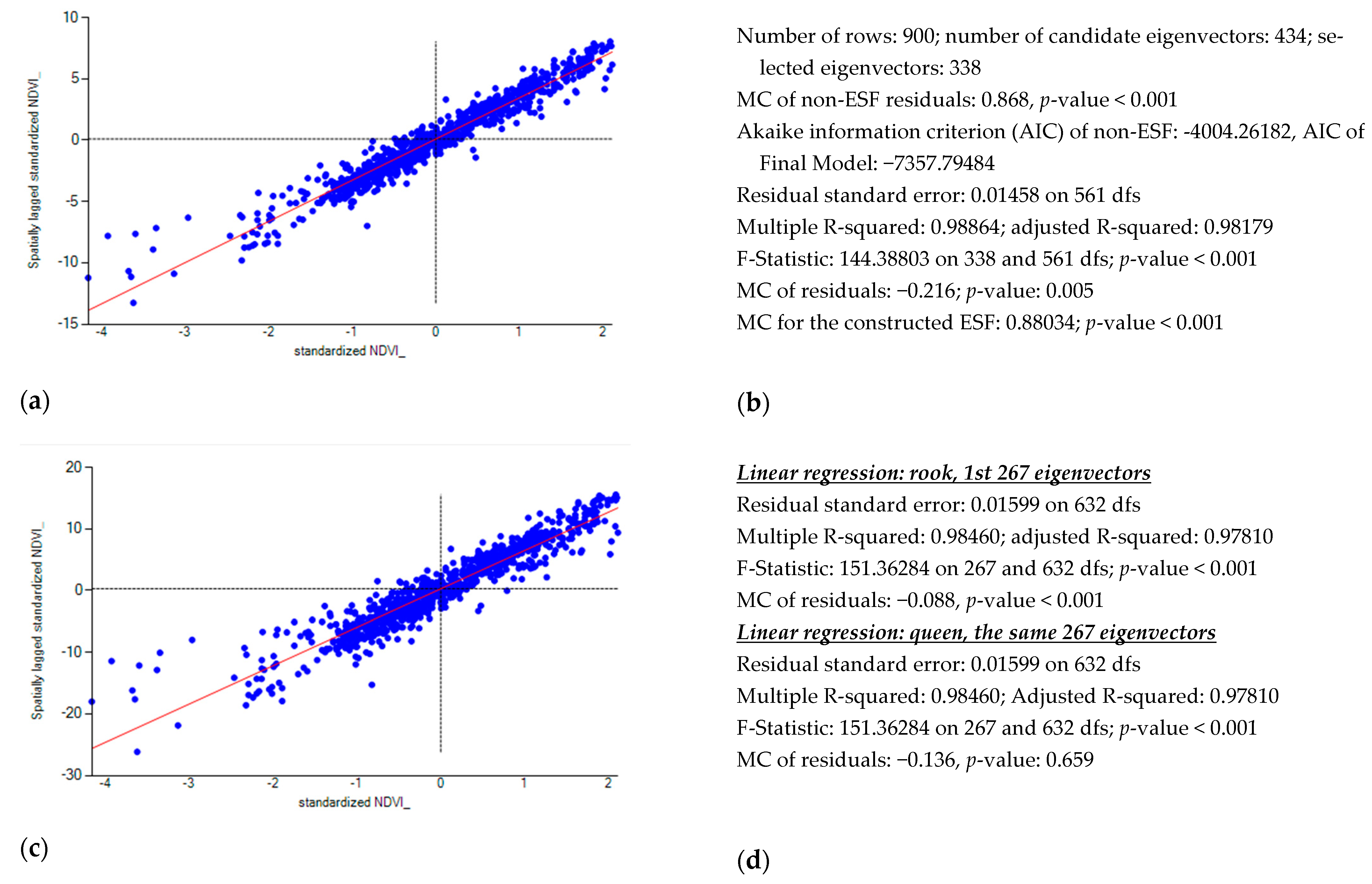
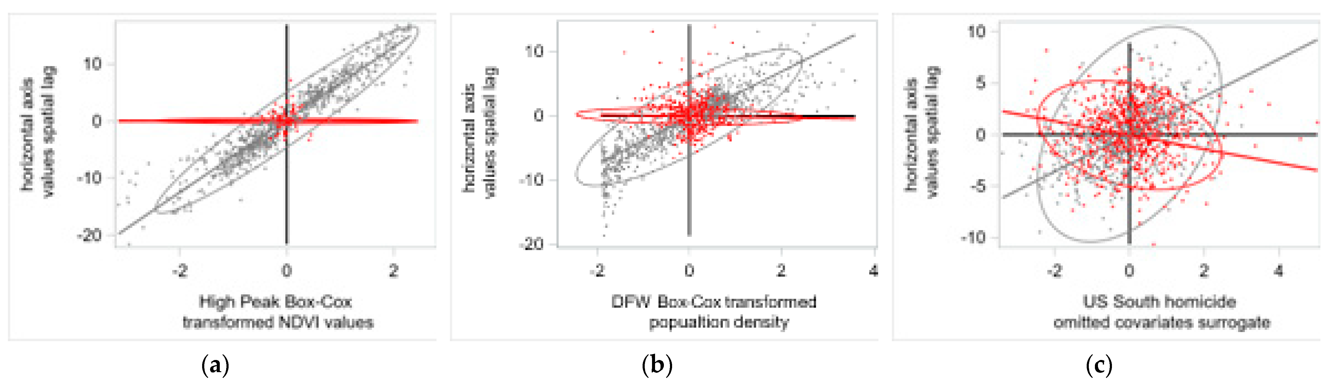
4.1. Remotely Sensed Data Results: The Case of Strong Positive SA

Numerous georeferenced phenomena studied to date display mostly or exclusively positive SA; therefore, spatial scientists almost always overlook and neglect negative SA [31]. Given that repetitious contrasts materializing in map patterns exhibiting negative SA tend to be elusive as well as confined in contiguous geographic landscapes, unable to materialize as easily as positive SA in more synchronized geographically continuous data, repeatedly negative SA is hidden, masked by dominant positive SA. Remotely sensed data illuminate this situation in a very interesting way through their regular square tessellation configuration. The original spatial resolution geographic distribution version of the preceding High Peak NDVI data (Figure 3a;) is across a 30-by-30 pixel mesh (i.e., a regular square tessellation forming a complete rectangular region). A simple SAR model specification description of these data, namely, for areal unit i,
y i = ρ j = 1 n w ij y j + ( 1 ρ ) μ + ε i ( i = 1 , 2 , , n ) ,
where y denotes NDVI, μ denotes the population mean of y, wij is the row-standardized version of cij (the most commonly used spatial weights specification in autoregressive models), and ε denotes a standard independent and identically distributed statistical random error term, produces two notable results: for a binary 0–1 cij rook definition of adjacency, a SA parameter estimate, ρ ^ , of 0.989 ( s ρ ^ ≈ 0.005), which is >0.9+, and an approximate residual MC of 0.172 (sMC ≈ 0.024; MCmax = 1.02) and GR of 0.813 (sGR ≈ 0.053)—computed as ei = ε ^ i = yi − [ ρ ^ j = 1 n w ij y j + (1 − ρ ^ ) μ ^ ]—implying the continued presence of more than trace positive SA in the spatial regression residuals, ei; and, for a cij queen definition of adjacency, a SA parameter estimate, ρ ^ , of 0.990 ( s ρ ^ ≈ 0.005), which again is >0.9+, and an approximate residual MC of 0.156 (sMC ≈ 0.017; MCmax = 1.03) and GR of 0.810 (sGR ≈ 0.051), once more implying the continued presence of more than trace positive SA in the spatial regression residuals, ei. This comparison implies that the remaining residual SA is not a function of the SWM definition.
Extending the SAR to the SARMA specification for the High Peak NDVI example, namely,
y i = ρ j = 1 n w ij y j + ( 1 ρ ) μ + θ j = 1 n w ij ε j + ε i ( i = 1 , 2 , , n ) ,
the rook adjacency-based parameter estimates become ρ ^ ≈ 0.966 ( s ρ ^ ≈ 0.009), a slight decrease in its magnitude, with an accompanying MA parameter estimate, θ ^ , of −0.389 ( s θ ^ ≈ 0.042)—indicating positive SA because the sign of a MA parameter is the opposite of its SA nature—and an approximate residual MC of 0.013 (sMC ≈ 0.024) and GR of 0.971 (sGR ≈ 0.053), implying the presence of only a trace amount of residual SA for this second specification. These estimates confirm that positive SA is in excess of 0.9 (the average lag-1 spatial correlation is roughly 0.93). Furthermore, the queen adjacency-based parameter estimate becomes ρ ^ ≈ 0.949 ( s ρ ^ ≈ 0.014), a slight decrease in its magnitude, with an accompanying MA parameter estimate, θ ^ , of −0.684 ( s θ ^ ≈ 0.072), and an approximate residual MC of 0.014 (sMC ≈ 0.017) and GR of 0.948 (sGR ≈ 0.051), again implying the presence of only a trace amount of residual SA for this second specification. These estimates also confirm that positive SA exceeds 0.9 (the average lag-1 spatial correlation is roughly 0.92). In other words, for these remotely sensed data, neither a SWM nor a model specification extension uncovers a negative SA component (i.e., no detection of a mixture); rather, these extensions further emphasize that the degree of positive SA latent in remotely sensed images tends to be marked.
This simple autoregressive (i.e., SAR) residual SA removal failure typifies many remotely sensed datasets, in part because they contain such extremely high positive SA levels. Getis and Ord [56] provide another publicly available empirical example reproducing this situation, a 16-by-16 specimen image with a single remotely sensed variable, the grey scale value (i.e., integers in the closed interval [20 − 1, 28 − 1] = [0, 255]) for each pixel. Its simple SAR model specification coupled with a rook adjacency definition yields the SA parameter estimate ρ ^ ≈ 0.964 ( s ρ ^ ≈ 0.014), which, again, slightly decreases to 0.891 by including a companion MA parameter, whose estimate is θ ^ ≈ −0.654 ( s θ ^ ≈ 0.061). The accompanying approximate residual MC decreases from 0.221 (sMC ≈ 0.046) to 0.013, with the corresponding GR increasing from 0.801 (sGR ≈ 0.100) to 1.011, implying nothing more than a trace amount of residual SA being present in this second specification, and again confirming that marked positive SA tends to characterizes remotely sensed data.
A rational supposition is that vegetation reflected in NDVI values should be accompanied by a positive–negative SA mixture hypothesis. Vegetation engages in geographic competition for sunlight, moisture, and soil nutrients, among other factors, implying a negative SA linkage for it; remotely sensed image pixels resemble Figure 4a,e, but engage in an abstract (e.g., seizing/squandering nearby moisture) rather than concrete tabs-and-slots type of spatial competition. Vegetation also simultaneously engages in synchronous geographic behavior by types of vegetation clustering due to seeding processes, accompanied by similar biological needs for geographically patterned sunlight, moisture, soil type, and soil nutrients, among other factors, implying a positive SA linkage for it. Therefore, the geographic distribution of NDVI should be characterized by a positive–negative SA mixture. The preceding autoregressive analyses fail to uncover this mixture, in part because sometimes positive SA is so dominant that negative SA becomes hidden [57]. Using MESF methodology, and retaining the rook definition of geographic adjacency, yields a 267-eigenvector SA description (from a candidate set of 434 vectors) for the Box–Cox transformed High Peak NDVI response variable that accounts for 98.4% of its geographic variance across 900 pixels. As with the preceding autoregressive residuals, the MESF linear regression specification, namely
yi = μ + ESFPSA,i + ESFNSA,i + εi (i = 1, 2, …, n),
where ESFPSA and ESFNSA respectively denote the positive and negative SA ESF (i.e., weighted sums of synthetic SA variates) components, renders residuals containing more than trace SA (its null hypothesis zMC ≈ 5.7 and zGR ≈ −3.0). Replacing the SWM in this probe with one defined by a queen’s adjacency definition results in MC = 0.84 (MCmax = 1.03) and GR = 0.13, converting 53 of the selected eigenvectors to ones representing negative rather than positive SA, although they account for a mere 1.2% of the NDVI geographic variance; an important consequence of this definitional change is the presence of only trace residual SA (its null hypothesis zMC ≈ −0.6 and zGR ≈ −0.5). This MESF finding confirms the existence of a positive–negative SA mixture, with the negative SA component hidden. Figure 7 displays selected akin ESF Tool output for this data analysis; these results require some post-processing to match their SAS counterparts reported in this paragraph (Step 1: save the 338 eigenvectors selected by the “Eigenvector Spatial Filtering Regression” option. Step 2: use the first 267 of these eigenvectors in a “Linear Regression” option, testing the residual SA with the binary 0–1 rook SWM. Step 3: repeat Step 2 testing with the binary 0–1 queen SWM).

4.2. Socio-Economic/Demographic Data Results: The Case of Moderate Positive SA

Figure 8 furnishes a socio-economic/demographic data example, portraying the Box–Cox transformed population density geographic distribution, with n = 1314 census tracts; the two DFW subcenters are somewhat conspicuous in this graphic. Urban economics conceptualizations and theory postulate that such metropolitan population density should contain positive SA, in part because similar land uses cluster in geographic space; it also postulates that metropolitan population density should contain negative SA, due to land use competition (a la von Thünen/Alonso). Output for this example is consistent with these expectations. Employing a SWM rook adjacency definition, the SAR model specification description of these transformed population density data produces a positive correlation of roughly 0.5, and implies the presence of little more than trace SA based upon its residual MC (Table 1). SARMA and a queen adjacency definition (which increases its SWM number of linkages by approximately 20%) fail to alter this more parsimonious conclusion. The GR, which statistically is less powerful than the MC, suggests that a small amount of SA may remain in the autoregression residuals; the SARMA estimates indicate that any residual SA remaining indeed is negative. In other words, a positive–negative SA mixture characterizes these Box–Cox transformed population density data, with the positive dominating the negative SA component.
Table 2 corroborates this positive–negative SA mixture verdict. Positive SA rook adjacency outcomes (Figure 8c) imply the presence of little more than trace residual SA, with essentially consistent MC and GR inferences. Adding a negative SA component accounts for very little additional geographic variance, at a cost of poorer residual SA diagnostic statistics. However, these deteriorated statistics build upon a −0.06 observed MCf, whose expected value is −0.10; especially this observed MC magnitude substantively is inconsequential. Switching to the queen adjacency definition renders comparable outcomes.
Likewise, geography of crime conceptualizations allow for crime rates to contain a mixture of positive and negative SA, the former correlating with locational attributes that attract crime to places, and the latter correlating with displacement of crime to nearby places due to local law enforcement. Griffith [31] presents a county level (n = 1412) spatial statistical reanalysis of homicide rates across the southern United States (US). He discovered in his evaluation that the omitted variables surrogate covariate—a random effects term—he included contains a mixture of positive and negative SA. MESF methodology furnishes the foundation for his published treatment. Table 3 summarizes output from its autoregressive assessment counterpart, which corroborates the positive–negative SA mixture uncovered by the MESF analysis.

4.3. Case Studies Discussion

SA already has a plurality of faces. Of the eight renditions widely acknowledged at present, for all practical purposes, arguments in this paper dismiss the nuisance interpretation because SA matters (as most quantitative geographers and other spatial scientists recognize today), replacing it with a newly emerging interpretation that often latent SA in georeferenced data is a mixture of positive and negative SA, and supplementing it with an additional interpretation that moderate positive (net) SA epitomizes most socio-economic/demographic, whereas very strong positive (net) SA epitomizes most remotely sensed image, geographic distributions. The jigsaw puzzle metaphor demonstrates this former conjecture, whereas empirical evidence encapsulated in the preceding section supports this latter conjecture, with implications about solving more difficult jigsaw puzzles (e.g., more pieces, and/or more highly complex pictures).
Figure 9 further illuminates the positive–negative SA mixture notion, accentuating that positive SA can mask negative SA; all three Moran scatterplots, which in their standard form fail to differentiate between positive and negative SA, highlight that the negative SA component spans the second and forth quadrants (i.e., H-L and L-H pairings) while concentrating around each graph’s origin. As the High Peak empirical example shows, although a mixture’s negative SA is hidden sometimes (the corresponding linear regression line slope in Figure 9a is nearly zero), overlooking it in an analysis produces poor diagnostic statistics (e.g., omitted variables bias). The DFW and US South empirical examples show that as a scattering of points disperses further into the second and fourth quadrants, the prominence of its negative SA component increases.
Perhaps the most crucial and profound revelation the jigsaw puzzle metaphor motivates is construction of positive and negative SA Moran scatterplot trendline pairs, which serendipitously demonstrates graphically for the first time that the negative SA slopes typically are much shallower than their positive SA accompaniments in these mixtures; negative SA almost always is weaker and therefore tends to be much less salient. This is a critical fact from the omitted variables bias perspective, especially when many covariates have enhanced pairwise correlations due to SA. Even a variable that does not have a strong relationship with a model’s response variable itself can cause big issues when it is omitted and there is some degree of correlation between it and several of the other variables included in the model. Hopefully the jigsaw puzzle metaphor can spawn other insights.

5. Summary, Conclusions, and Implications

SA is everywhere, and its constant encountering requires a keener awareness as well as an improved understanding of it. In turn, improved SA comprehension can contribute to such endeavors as “develop[ing] and offer[ing] new strategies, visions and proposals on the role of sustainability and resilience related to urban and rural contexts” [1], such as spatially adjusted analytical techniques, or “help[ing] policy-makers to manage the new chances set up by a particularly complex and dynamic socioeconomic scenario worldwide” [1], such as furnishing appropriate tools for monitoring and evaluating sustainability progress. To these ends, this paper makes the following two contributions: (1) establishing the jigsaw puzzle metaphor for explaining in relatively simple and intelligible terms the concept of SA; and, (2) the additional interpretation of SA as frequently being a mixture of positive and negative local geographic relationships (supplementing [32,33]). Within the confines of this second knowledge advancement, this paper presents a conjecture that positive SA dominates the vast majority of geographic distributions, characterizing most remotely sensed images with marked degrees, and characterizing most socio-economic/demographic phenomena as having moderate degrees. Spatial statistical tools uncover evidence corroborating these contentions, uncovering hidden negative SA among marked positive SA in remotely sensed images, and exposing negative residual SA among moderate positive SA in population density and homicide rates.
One drawback of the jigsaw puzzle metaphor is that it limits a discussion to mutually exclusive and collectively exhaustive 2-D area dissections of geographic landscapes, partitionings largely artificial (e.g., administrative boundaries) in the real world. A variety of other metaphors show potential, at least in terms of supplementing the jigsaw puzzle. The 2-D 4-by-8 grid layout synchronized black-orange-red metronomes experiment (e.g., https://www.youtube.com/watch?v=5v5eBf2KwF8 (accessed on 24 August 2023)) emphasizes the connection between synchronization and positive SA, supplies a common factor source of SA as well as point location attributes, and illustrates a positive SA range extending from near zero to near one. Insect behavior, such as the flashing lights pattern of synchronous fireflies (e.g., https://insidescience.org/news/how-synchronize-fireflies (accessed on 24 August 2023)), provides a spatial interaction source of SA, again ranging from near random (initial flashes) to near perfect (flashings appears to occur at the same time) SA. Noteworthy here is that Heckscher [59] discovered a new firefly species by recognizing deviations from the well-known SA flashing pattern, demonstrating the power of SA. Reminiscent of the Schelling [60,61] model, which deals with a mixture of point and polygon areal units, The Economist [62] notes that positive SA rather than a random mixture of household opinions, tends to characterize places:
The north [of England] has wealthy suburbs, like South Wirral, west of Liverpool. They vote Labour. The south has impoverished pockets, like north-east Kent. They vote Conservative. It is as though political opinions derive from the air people breathe.
Recent scholarly inquires reporting that, for example, US households often migrate to places matching their politics [63], and anti-vaccine sentiment tends to geographically concentrate [64], corroborate this geographical clustering contention. Artistic paintings deliver yet another conceivable metaphor (e.g., [65]; the fourth in a sequence of papers about this topic that spans five years): SA is latent in the red–green–blue (RGB) spectral band color channels of artists’ paintings, with MESF methodology capable of producing painting replications that visibly are nearly indistinguishable from their original artwork. This incomplete review of possible alternative metaphors exemplifies that: (1) many more metaphors exist, but apparently solely for the most common case of positive SA; (2) other potential metaphors appear to be inferior to the one furnished by jigsaw puzzles because they fail to illustrate negative or mixtures of SA; and, (3) the jigsaw puzzle, from its inception through to its many contemporary and sometimes subtly different versions (e.g., tangrams, slider puzzles), furnishes a fathomable metaphor for understanding SA.
Therefore, one conclusion is that the jigsaw puzzle metaphor furnishes a superior and ideal pedagogic tool for comprehending SA. A second conclusion is that autoregressive and moving average parts of a SARMA model specification usually are highly correlated, although they fail to reach the troublesome level of ±0.95, at least for the empirical examples presented in this paper; nevertheless, particularly because this threshold comes from time series practice, the interval (0.8, 0.9) may well raise some concerns for spatial series practice. Otherwise, an alternative conclusion suggested by the SARMA results is that the degree of positive SA in economic/demographic phenomena also is marked, with a considerable amount of it offset by its (near-)universal accompanying negative SA when indexed by a single quantifier, rendering a perceptible moderate degree of net SA. Another prominent conclusion is that negative SA merits substantially more study attention by spatial scientists [31].
Finally, a critical implication is that zero SA rarely exists, except in a net positive–negative mixture. Accordingly, Figure 9 implies that the utility of the Moran scatterplot in its present form may be seriously compromised. An additional implication is that MESF methodology allows a more efficient and effective investigation of positive–negative SA mixtures than is afforded by autoregressive methodology, alone. These various implications warrant subsequent research consideration.

Funding

This research received no external funding.

Data Availability Statement

Except for the easily simulated data (Figure 2 utilized Minitab pseudo-random number generator values), all other data are publicly available, and retrievable from on-line sources.

Acknowledgments

The author is an Ashbel Smith Professor of Geography and Geospatial Information Sciences. He thanks Qing Luo (Wuhan Institute of Technology) for providing the earlier version of her collaborative graphic appearing in Figure 1.

Conflicts of Interest

The authors declare no conflict of interest.

References

  1. Salvati, L. Editorial: Introduction to a new open access journal by MDPI. Geographies 2020, 1, 1–2. [Google Scholar] [CrossRef]
  2. Griffith, D. Spatial autocorrelation is everywhere. In Our Geographical Worlds: Celebrating Award-Winning Geography at the University of Toronto 1995 to 2018; Macijauskas, J., Ed.; Department of Geography and Planning & Association of Geography Alumni, University of Toronto: Toronto, ON, Canada, 2022; pp. 1–11. [Google Scholar]
  3. Tobler, W. A computer movie simulating urban growth in the Detroit region. Econ. Geogr. 1970, 46, 234–240. [Google Scholar] [CrossRef]
  4. Williams, A. The Jigsaw Puzzle: Piecing Together a History; Berkley Books: New York, NY, USA, 2004. [Google Scholar]
  5. Monmonier, M. Air Apparent: How Meteorologists Learned to Map, Predict, and Dramatize Weather; University of Chicago Press: Chicago, IL, USA, 2000. [Google Scholar]
  6. Student. The elimination of spurious correlation due to position in time or space. Biometrika 1914, 10, 179–180. [Google Scholar]
  7. Yule, U. Why do we sometimes get nonsense-correlations between time series? A study in sampling and the nature of time series. J. R. Stat. Soc. 1926, 89, 1–69. [Google Scholar] [CrossRef]
  8. Neprash, J. Some problems in the correlation of spatially distributed variables. Proc. Am. Stat. J. 1934, 29, 167–168. [Google Scholar]
  9. Stephan, F. Sampling errors and interpretations of social data ordered in time and space. Proc. Am. Stat. J. 1934, 29, 165–166. [Google Scholar]
  10. Fisher, R. The Design of Experiments; Oliver and Boyd: Edinburgh, UK, 1935. [Google Scholar]
  11. Yates, F. The comparative advantages of systematic and randomized arrangements in the design of agricultural and biological experiments. Biometrika 1938, 30, 444–466. [Google Scholar]
  12. Moran, P. Notes on continuous stochastic phenomena. Biometrika 1950, 37, 17–23. [Google Scholar] [CrossRef]
  13. Geary, R. The contiguity ratio and statistical mapping. Inc. Stat. 1954, 5, 115–145. [Google Scholar] [CrossRef]
  14. Cliff, A.; Ord, J. Spatial Autocorrelation; Pion: London, UK, 1973. [Google Scholar]
  15. Journel, A.; Huijbregts, C. Mining Geostatistics; Academic Press: New York, NY, USA, 1978. [Google Scholar]
  16. Paelinck, J.; Klaassen, L. Spatial Econometrics; Saxon House: Farnborough, UK, 1979. [Google Scholar]
  17. Anselin, L. Spatial Econometrics; Kluwer: Dordrecht, Germany, 1988. [Google Scholar]
  18. Cressie, N. Statistics for Spatial Data; Wiley: New York, NY, USA, 1991. [Google Scholar]
  19. Haining, R. Spatial Data Analysis in the Social and Environmental Sciences; Cambridge University Press: Cambridge, UK, 1996. [Google Scholar]
  20. Anselin, L. Local indicators of spatial association LISA. Geogr. Anal. 1995, 27, 93–115. [Google Scholar] [CrossRef]
  21. Griffith, D. A family of correlated observations: From independent to strongly interrelated ones. Stats 2020, 3, 166–184. [Google Scholar] [CrossRef]
  22. Goodchild, M. Spatial Autocorrelation; Concepts and Techniques in Modern Geography 47; Geo Books: Norwich, UK, 1986. [Google Scholar]
  23. Odland, J. Spatial Autocorrelation; SAGE: Thousand Oaks, CA, USA, 1988. [Google Scholar]
  24. Getis, A. A history of the concept of spatial autocorrelation: A geographer’s perspective. Geogr. Anal. 2008, 40, 297–309. [Google Scholar] [CrossRef]
  25. Goodchild, M. What problem? Spatial autocorrelation and geographic information science. Geogr. Anal. 2009, 41, 411–417. [Google Scholar] [CrossRef]
  26. Griffith, D. What is spatial autocorrelation? Reflections on the past 25 years of spatial statistics. L’Espace Géographique 1992, 21, 265–280. [Google Scholar] [CrossRef]
  27. Haining, R. Spatial autocorrelation and the quantitative revolution. Geogr. Anal. 2009, 41, 364–374. [Google Scholar] [CrossRef]
  28. Legendre, P. Spatial autocorrelation: Trouble or new paradigm? Ecology 1993, 74, 1659–1673. [Google Scholar] [CrossRef]
  29. McMillen, D. Spatial autocorrelation or model misspecification? Int. Reg. Sci. Rev. 2003, 26, 208–217. [Google Scholar] [CrossRef]
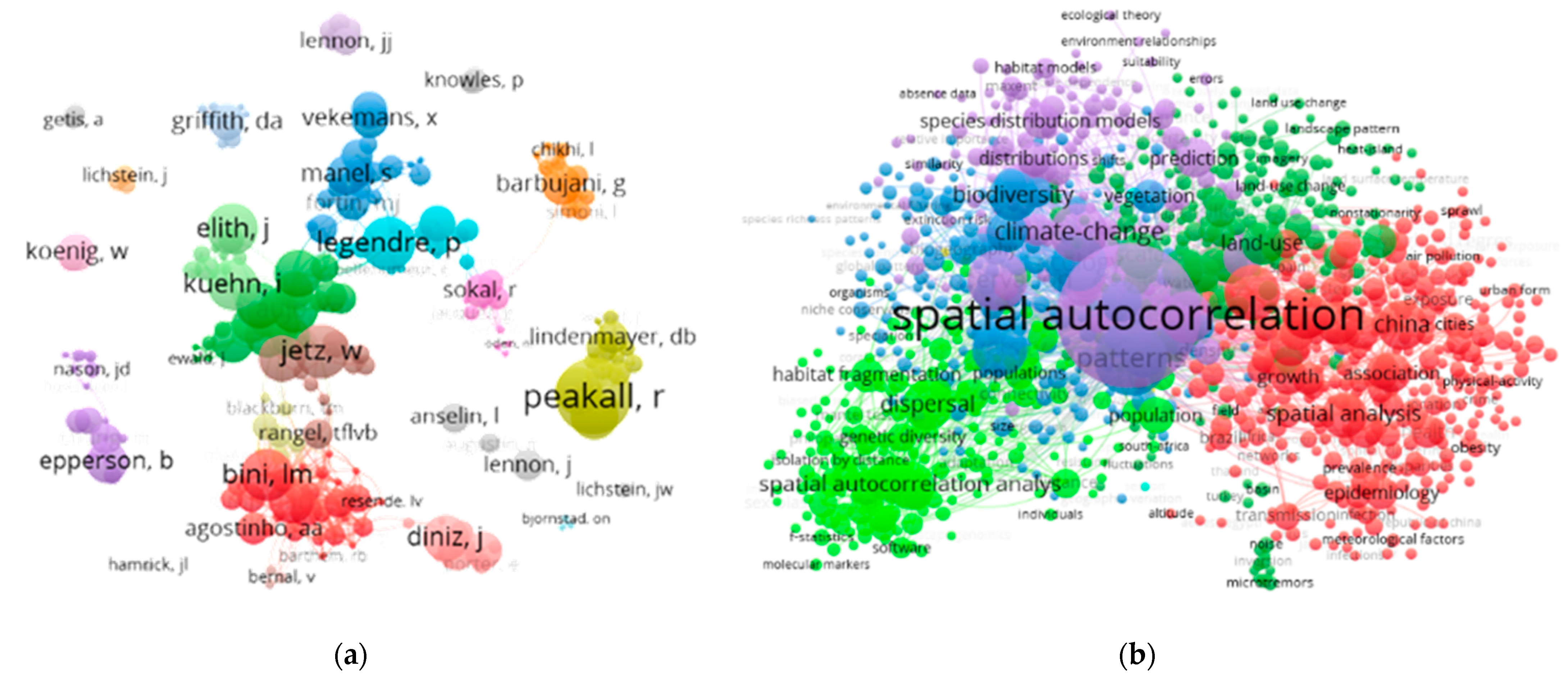
  30. Luo, Q.; Hu, K.; Liu, W.; Wu, H. Scientometric analysis for spatial autocorrelation-related research from 1991 to 2021. ISPRS Int. J. Geo-Inf. 2022, 11, 309. [Google Scholar] [CrossRef]
  31. Griffith, D. Negative spatial autocorrelation: One of the most neglected concepts in spatial statistic. Stats 2019, 2, 388–415. [Google Scholar] [CrossRef]
  32. Griffith, D.; Agarwal, K.; Chen, M.; Lee, C.; Panetti, E.; Rhyu, K.; Venigalla, L.; Yu, X. Geospatial socio-economic/demographic data: The existence of spatial autocorrelation mixtures in georeferenced data—Part I & Part II. Trans. GIS 2022, 26, 72–99. [Google Scholar]
  33. Griffith, D. Spatial autocorrelation mixtures in geospatial disease data: An important global epidemiologic/public health assessment ingredient? Trans. GIS 2023, 27, 730–751. [Google Scholar] [CrossRef]
  34. Griffith, D.; Chun, Y. Evaluating eigenvector spatial filter corrections for omitted georeferenced variables. Econometrics 2016, 4, 29. [Google Scholar] [CrossRef]
  35. Pawley, M.; McArdle, B. Spatial Autocorrelation: Bane or Bonus? bioRxiv. 2018. Available online: https://www.biorxiv.org/content/10.1101/385526v1.article-info (accessed on 24 August 2023).
  36. Chou, Y. Map resolution and spatial autocorrelation. Geogr. Anal. 1991, 23, 228–246. [Google Scholar] [CrossRef]
  37. Zhang, B.; Xu, G.; Jiaoa, L.; Liua, J.; Donga, T.; Lia, Z.; Liu, X.; Liu, Y. The scale effects of the spatial autocorrelation measurement: Aggregation level and spatial resolution. Int. J. Geogr. Inf. Sci. 2019, 33, 945–966. [Google Scholar] [CrossRef]
  38. Rodrigues, A.; Tenedorio, J. Sensitivity Analysis of Spatial Autocorrelation Using Distinct Geometrical Settings: Guidelines for the Urban Econometrician. In Computational Science and Its Applications—ICCSA 2014; Murgante, B., Murgante, B., Misra, S., Rocha, A., Torre, C., Rocha, J., Falcão, M., Taniar, D., Apduhan, B., Gervasi, O., Eds.; Part III, LNCS 8581; Springer: Cham, Switzerland, 2014; pp. 345–356. [Google Scholar]
  39. Di, W.; Qingbo, Z.; Zhongxin, C.; Jia, L. Spatial autocorrelation and its influencing factors of the sampling units in a spatial sampling scheme for crop acreage estimation. In Proceedings of the 6th International Conference on Agro-Geoinformatics, Fairfax, VA, USA, 7–10 August 2017; pp. 1–6. [Google Scholar] [CrossRef]
  40. Mohan, P.; Zhou, X.; Shekhar, S. Quantifying resolution sensitivity of spatial autocorrelation: A resolution correlogram approach. In Geographic Information Science: GIScience 2012; Xiao, N., Kwan, M.-P., Goodchild, M., Shekhar, S., Eds.; Lecture Notes in Computer Science; Springer: Berlin/Heidelberg, Germany, 2012; Volume 7478, pp. 132–145. [Google Scholar] [CrossRef]
  41. Armstrong, B. Jigsaw puzzle cutting styles: A new method of classification. In Game Researchers’ Notes; American Game Collectors Association: Dresher, PA, USA, 1997. [Google Scholar]
  42. Bailey, T.; Gatrell, A. Interactive Spatial Data Analysis; Longman: Harlow, UK, 1995. [Google Scholar]
  43. Brualdi, R. Introductory Combinatorics, 5th ed.; Pearson: Upper Saddle, NJ, USA, 2010. [Google Scholar]
  44. Numbla, N. Automatic Jigsaw Puzzle Solver. 2015. Available online: https://nithyanandabhat.weebly.com/uploads/4/5/6/1/45617813/project_report-jigsaw-puzzle.pdf (accessed on 24 August 2023).
  45. Guerroui, N.; Séridi, H. Solving computational square jigsaw puzzles with a novel pairwise compatibility measure. J. King Saud Univ. Comput. Inf. Sci. 2020, 32, 928–939. [Google Scholar] [CrossRef]
  46. Eaton, B.; Lipsey, R. The non-uniqueness of equilibrium in the Löschian economic model. Am. Econ. Rev. 1976, 66, 77–93. [Google Scholar]
  47. Bunge, W. Theoretical Geography, 2nd ed.; Gleerup: Lund, Sweden, 1966. [Google Scholar]
  48. Lebart, L. Analyse statistique de la contiguite. Publ. L’institute Stat. L’universite Paris 1969, 18, 81–112. [Google Scholar]
  49. Diniz-Filho, J.; Bini, L.; Hawkins, B. Spatial autocorrelation and red herrings in geographical ecology. Glob. Ecol. Biogeogr. 2003, 12, 53–64. [Google Scholar] [CrossRef]
  50. Kao, Y.-H.; Bera, A. Spatial Regression: The Curious Case of Negative Spatial Dependence. In Proceedings of the IV International Scientific Conference: Spatial Econometrics and Regional Economic Analysis, Lodz, Poland, 13–14 June 2016; Kao, Y.-H., Three Essays on Spatial Econometrics with an Emphasis on Testing, unpublished doctoral dissertation; Department of Economics, University of Illinois at Urbana-Champaign: Urbana, IL, USA, 2016. [Google Scholar]
  51. Griffith, D.; Chun, Y.; Li, B. Spatial Regression Analysis Using Eigenvector Spatial Filtering; Elsevier: Cambridge, MA, USA, 2019. [Google Scholar]
  52. Griffith, D. Spatial Autocorrelation and Spatial Filtering: Gaining Understanding through Theory and Scientific Visualization; Springer: Berlin/Heidelberg, Germany, 2003. [Google Scholar]
  53. Koo, H.; Chun, Y.; Griffith, D. Integrating spatial data analysis functionalities in a GIS environment: Spatial analysis using ArcGIS Engine and R (SAAR). Trans. GIS 2018, 22, 721–736. [Google Scholar] [CrossRef]
  54. Griffith, D. Eigenfunction properties and approximations of selected incidence matrices employed in spatial analyses. Linear Algebra Its Appl. 2000, 321, 95–112. [Google Scholar] [CrossRef]
  55. Cliff, A.; Ord, J. Spatial Processes; Pion: London, UK, 1981. [Google Scholar]
  56. Getis, A.; Ord, J. Local spatial statistics: An overview. In Spatial Analysis: Modelling in a GIS Environment; Longley, P., Batty, M., Eds.; Geoinformation International: Cambridge, UK, 1996; pp. 261–277. [Google Scholar]
  57. Griffith, D. Hidden negative spatial autocorrelation. J. Geogr. Syst. 2006, 8, 335–355. [Google Scholar] [CrossRef]
  58. Arbia, G. Spatial Econometrics; Springer: Berlin/Heidelberg, Germany, 2006. [Google Scholar]
  59. Heckscher, C. Photuris Mysticalampas (Coleoptera: Lampyridae): A new firefly from peatland floodplain forests of the Delmarva Peninsula. Entomol. News 2013, 123, 93–100. [Google Scholar] [CrossRef]
  60. Schelling, T. Models of segregation. Am. Econ. Rev. 1969, 59, 488–493. [Google Scholar]
  61. Schelling, T. Dynamic models of segregation. J. Math. Sociol. 1971, 1, 143–186. [Google Scholar] [CrossRef]
  62. The Economist. Britain’s Great Divide: The Politics of North and South; The Economist: London, UK, 2013; Volume 407, p. 16. [Google Scholar]
  63. Liu, X.; Andris, C.; Desmarais, B. Migration and political polarization in the U.S.: An analysis of the county-level migration network. PLoS ONE 2019, 14, e0225405. [Google Scholar] [CrossRef]
  64. Igraham, C. California’s Epidemic of Vaccine Denial, Mapped. The Washington Post 27 January 2015. Available online: https://www.washingtonpost.com/news/wonk/wp/2015/01/27/californias-epidemic-of-vaccine-denial-mapped/ (accessed on 24 August 2023).
  65. Griffith, D. Eigenvector visualization and art. J. Math. Arts 2021, 15, 170–187. [Google Scholar] [CrossRef]
Figure 1. Web of Science (2012–2018) SA keyword cloud infographics (arbitrary group coloring visually differentiates among perceived SA research communities; node size reflects weighted normalized citation counts, which tend to highlight leading community scholars); compilation and portrayals by Drs. Kai Hu (Jiangnan University) and Qing Luo (Wuhan Institute of Technology). Left (a): authors. Right (b): concepts.
Geographies 03 00028 g001
Figure 2. Specimen Moran scatterplots portraying the different natures and degrees of SA (n = 25) using z-score axes; gray lines denotes 95% confidence intervals, red lines denote 95% prediction intervals, blue denotes the origin axes, and black denotes trend lines. Left (a): positive (Figure 3b), MC ≈ 0.44, Geary Ratio (GR; a popular paired comparisons (i.e., squared differences in neighboring attribute values) SA index) ≈ 0.52. Middle (b): zero (Figure 3d), MC ≈ −0.03, GR ≈ 0.98. Right (c): negative (Figure 3c), MC ≈ −0.45, GR ≈ 1.42.
Geographies 03 00028 g002
Figure 3. A specimen aggregated High Peak normalized difference vegetation index (NDVI; from [42]) remotely sensed image as a jigsaw puzzle; the green–yellow–red tertile color palate is directly proportional to the NDVI values (i.e., red denotes H, yH, yellow denotes M, yM, and green denotes L, yL, values). Left (a): the NDVI geographic distribution across a 30-by-30 pixels landscape (rook adjacency criterion; MC ≈ 0.88, GR ≈ 0.10, n = 900) overlaid with a five-by-five jigsaw puzzle dissection (i.e., cutting). Left middle (b): average NDVI values by puzzle piece (mimicking the visualization detected by an adjacent sight cones cluster in a human’s eye). Right middle (c): a Thiessen polygon overlay based upon puzzle piece centroids (puzzle piece physical centers computed by ESRI© ArcMap) to emphasize the tags and slots. Right (d): a random permutation of the (b) average values.
Geographies 03 00028 g003
Figure 4. Selected degree-of-difficulty jigsaw puzzle types; red vertical two-way arrows link unassembled puzzle pieces to their solutions. Top left (a): patterned square pieces. Bottom left (e): Figure 4a solution. Top left middle (b): blank square pieces (e.g., https://minifigs.me/products/draw-your-own-personalised-puzzle-various-sizes-custom-lego-jigsaw-puzzle). Bottom left middle (f): a possible (b) solution. Top right middle (c): blank irregular (i.e., random cut) shaped pieces (e.g., https:/www.aliexpress.us/item/2255799894529529.html?gatewayAdapt=glo2usa4itemAdapt) Bottom right middle (g): a possible (c) solution in progress. Top right (d): patterned irregularly shaped pieces. Bottom right (h): (d) solution.
Geographies 03 00028 g004
Figure 5. Ghostly spatial competition. Left (a): invisible hands creating an all-or-nothing square checkerboard attribute pattern. Middle (b): invisible hands (red) superimposed upon their coordinated physical tabs and slots. Right (c): illustrative invisible hands (red) protruding from the single 1st-level central place; seven (via nesting) 2nd-level central places offer a distinct bundle of goods/services that creates a have/have not hexagonal checkerboard mosaic.
Geographies 03 00028 g005
Figure 6. The 2010 geographic distribution of Box–Cox transformed percentage of occupied houses across the Dallas–Fort Worth (DFW) Metroplex census tracts. Left (a): 20 (i.e., four rows by five columns) jigsaw puzzle pieces (constructed using BookWidgets: https://www.bookwidgets.com/ widget-library/jigsaw-puzzle (accessed on 23 August 2023)). Right (b): the assembled jigsaw puzzle (MC ≈ 0.63, GR ≈ 0.37; rook adjacency definition).
Geographies 03 00028 g006
Figure 7. High Peak Box–Cox transformed NDVI SA computation results. Top left (a): a binary (i.e., 0–1) rook SWM Moran scatterplot. Top right (b): output from ESF Tool. Bottom left (c): a binary queen SWM Moran scatterplot. Bottom right (d): output from ESF Tool based upon the first 267 MESF linear regression selected eigenvectors, using binary rook and queen SWMs.
Geographies 03 00028 g007
Figure 8. 2010 Box–Cox transformed population density across the DFW Metroplex census tracts. Left (a): 200 (i.e., 20 rows by 10 columns) jigsaw puzzle pieces (constructed using BookWidgets: https://www.bookwidgets.com/widget-library/jigsaw-puzzle (accessed on 23 August 2023)). Middle (b): the assembled jigsaw puzzle (MC ≈ 0.46, GR ≈ 0.41). Right (c): the rook adjacency definition MESF approximation reproduction of (b).
Geographies 03 00028 g008
Figure 9. Moran scatterplots, based upon a rook adjacency definition, with superimposed positive and negative SA component trend lines and 95% prediction ellipses (respectively denoted by red and grey). Left (a): Box–Cox transformed High Peak NDVI. Middle (b) Box–Cox transformed DFW population density. Right (c): a US South omitted covariates surrogate.
Geographies 03 00028 g009
Table 1. Box–Cox transformed 2010 DFW population density (Figure 8b) spatial autoregressive estimation results.
FeatureRook Adjacency DefinitionQueen Adjacency Definition
SARSARMA SARSARMA
ρ ^ ( s ρ ^ )0.820 (0.017)0.954 (0.014)0.844 (0.017)0.940 (0.018)
θ ^ ( s θ ^ )00.498 (0.061)00.383 (0.075)
r ρ ^ , θ ^ 00.81200.826
Average lag-1 spatial correlation0.560.620.560.61
pseudo-R20.643 0.647
Residual zMC; residual zGR−2.0; 1.81.7; 0.5−1.0; 0.91.5; 0.1
NOTE: the MA SA parameter sign is the opposite of its nature, in keeping with Box–Jenkins notation (also see [58]).
Table 2. Box–Cox transformed 2010 DFW population density (Figure 8b) MESF estimation results.
FeatureRook Adjacency Definition (SWM Elements Sum = 7074; MCmax ≈ 1.175)Queen Adjacency Definition (SWM Elements Sum = 8494; MCmax ≈ 1.125)
YPSANSAPSA + NSAYPSANSAPSA + NSA
# eigenvectors0204 (385)66 (400)270 (785)0186 (365)41 (366)227 (731)
MC0.640.89−0.420.810.590.84−0.380.78
GR0.370.211.480.270.370.211.480.25
R200.7500.0520.80200.7300.0380.768
Residual zMC37.8−1.0 2.238.60.8 3.2
Residual zGR−14.30.7−1.2−14.5−0.3−2.0
NOTE: # denotes “the number of”; PSA and NSA respectively denote positive and negative SA; the candidate positive SA eigenvectors set size is the calculation result from [51]; rook MCPSA+NSA ≈ 0.93(0.89) + 0.05(−0.42) ≈ 0.81 and GRPSA+NSA ≈ 0.93(0.21) + 0.05(1.48) ≈ 0.27; queen MCPSA+NSA ≈ 0.94(0.84) + 0.03(−0.38) ≈ 0.78 and GRPSA+Nesdf ≈ 0.94(0.21) + 0.03(1.48) ≈ 0.25.
Table 3. Spatial autoregressive estimation results for homicide rates across the US South [31].
FeatureRook Adjacency Definition (SWM Elements Sum = 7700; MCmax ≈ 1.111)Queen Adjacency Definition (SWM Elements Sum = 8096; MCmax ≈ 1.152)
SARSARSM SARSARSM
ρ ^ ( s ρ ^ )0.585 (0.025)0.988 (0.005)0.593 (0.025)0.988 (0.005)
θ ^ ( s θ ^ )00.880 (0.022)00.877 (0.022)
r ρ ^ , θ ^ 00.80800.805
Average lag-1 spatial correlation0.310.380.310.39
pseudo-R20.326 0.326
Residual zMC−2.4−0.1−2.3−0.1
Residual zGR−0.2−1.1−0.4−1.3
NOTE: the MA SA parameter sign is the opposite of its nature, in keeping with Box–Jenkins notation (also see [58]).
Disclaimer/Publisher’s Note: The statements, opinions and data contained in all publications are solely those of the individual author(s) and contributor(s) and not of MDPI and/or the editor(s). MDPI and/or the editor(s) disclaim responsibility for any injury to people or property resulting from any ideas, methods, instructions or products referred to in the content.

