Abstract
There has been a growth in the number of composite indicator tools used to assess community risk, vulnerability, and resilience, to assist study and policy planning. However, existing research shows that these composite indicators vary extensively in method, selected variables, aggregation methods, and sample size. The result is a plethora of qualitative and quantitative composite indices to choose from. Despite each providing valuable location-based information about specific communities and their qualities, the results of studies, each using disparate methods, cannot easily be integrated for use in decision making, given the different index attributes and study locations. Like many regions in the world, the Arctic is experiencing increased variability in temperatures as a direct consequence of a changing planetary climate. Cascading effects of changes in permafrost are poorly characterized, thus limiting response at multiple scales. We offer that by considering the spatial interaction between the effects of permafrost, infrastructure, and diverse patterns of community characteristics, existing research using different composite indices and frameworks can be augmented. We used a system-science and place-based knowledge approach that accounts for sub-system and cascade impacts through a proximity model of spatial interaction. An estimated ‘permafrost vulnerability surface’ was calculated across Alaska using two existing indices: relevant infrastructure and permafrost extent. The value of this surface in 186 communities and 30 military facilities was extracted and ordered to match the numerical rankings of the Denali Commission in their assessment of permafrost threat, allowing accurate comparison between the permafrost threat ranks and the PVI rankings. The methods behind the PVI provide a tool that can incorporate multiple risk, resilience, and vulnerability indices to aid adaptation planning, especially where large-scale studies with good geographic sample distribution using the same criteria and methods do not exist.
1. Introduction
1.1. Effects of Thawing Permafrost on Arctic Communities
Permafrost is ground that remains below 0 °C for two or more consecutive years, making it frozen and a largely stable foundation for above-ground flora, fauna, and built infrastructure [1]. Common in the Arctic and sub-Arctic regions, current estimates suggest that between 30% and 85% of current subsurface permafrost will thaw if current warming trends continue [2,3,4]. The effects of permafrost thaw are most visually striking on natural and artificial terrain features, e.g., the development of thermokarst, increases in the frequency and severity of thaw slump, damage to structures that experience stress as the ground becomes less stable, etc. [5,6,7,8,9].
However, permafrost thaw impacts extend well beyond these obvious examples, altering local hydrology, water chemistry, plant cover, and other characteristics and processes of the natural environment [10,11,12]. The cascade of outcomes threatens Arctic peoples both physically and culturally, which has spawned a body of research focused on how those living in the Arctic can assess and manage risk, and preserve their heritage and communities in the face of rapid change [13,14,15]. This has not been limited solely to the Arctic, and has been reflected in the expansion of indices worldwide—unevenly applied, and hard to directly compare—to assess risk, vulnerability, and resilience (Figure 1) [16].

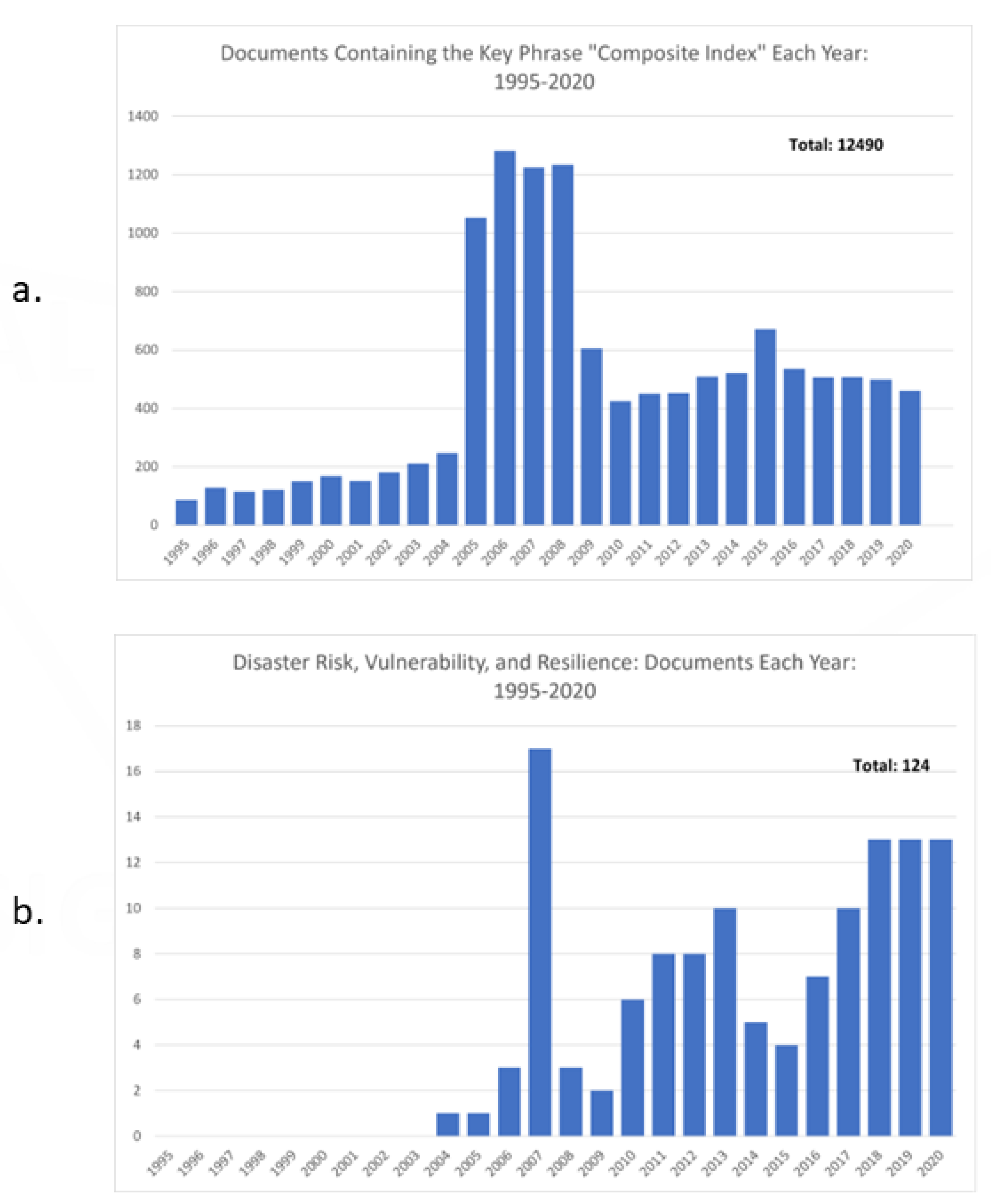
Figure 1.
(a) (top) shows the number of documents, each year, in which the key phrase “composite index” appears. (b) is the number of documents each year containing one or more of the following key phrases: “disaster risk index”, “disaster vulnerability index”, “disaster resilience index”, “community risk index”, “community vulnerability index”, “community resilience index”. The charts were produced using the results of ITHAKA’s Constellate service at https://constellate.org/builder, and presented here under their terms and conditions of permitted use, accessed 10 August 2023.
1.2. National Security Implications of Permafrost Thaw
While change and thaw of permafrost impacts food and environmental security in the Arctic, there is an increasing awareness of concerns and connections between permafrost degradation and national security. The role of the Arctic in geopolitical matters related to the Russian Federation has been extensively discussed since the Seward purchase of Alaska by the USA from Russia in 1867. Other nations, including those which identify as “near arctic”, such as China, assert a long history of exploration. It is only recently, however, that the Arctic has come to bear on national security and defense at a global scale as climate change makes it more accessible and its relatively unique geographic features (e.g., the shortest distances between landmasses in the northern hemisphere, etc) prove increasingly attractive to national defense entities. From impacts on military infrastructure [17], major communication cables [18], geoengineering security [19], and arctic operability [20], to risks for the geo-political situation in the Arctic [21], there is an urgent need for tools to support the mitigation of permafrost’s impacts on critical infrastructure, community livelihoods, and national security.
A large body of literature exists on climate change and the maritime domain that includes economic, military, security, public safety, subsistence, research, exploration and tourism [22,23,24,25]. Another considerable body of literature exists on the physics, engineering, and hydrology of the cryosphere including permafrost and its thaw [2,8,26]. Much of the literature on adaptation falls into two categories: large scale, pan-Arctic assessments and structure-scale engineering assessments. As with hydrological studies, especially local freshwater systems, the inclusion of sociocultural elements was lacking. And, notably, the treatment of national defense and security tends to focus on discussions of conflict or sovereignty (governance). Key concerns and connections between permafrost thaw and national security include: impacts on military infrastructure [17] and major communications cables [18]; geoengineering security [19]; Arctic operability and environmental security [20]; and national security interests and geopolitics of the Arctic [21].
In terms of public safety and security, both U.S. and Canadian defense and public safety agencies provide Arctic residents the support of activities such as search and rescue (SAR) and humanitarian assistance and disaster response (HADR). Given the rapid increases in climate variability, HADR may be expected to occur more frequently and requires a reliable set of infrastructure systems (e.g., airfields) to execute. From a national defense perspective, such infrastructure allows the U.S., Canada, and their allies to maintain a regular presence which improves our ability to detect, deter, and defend against threats, if necessary. Law enforcement and other public safety agencies also rely on a stable infrastructure system not only for movement and missions but also for the funding that sustains their organizations and activities. Alaska is already a difficult region to operate in for such agencies and, as permafrost thaw affects terrestrial systems, their missions will not only become more burdensome but also more expensive.
1.3. Evaluating Risk, Vulnerability, and Resilience
Existing methods for evaluating risk, vulnerability, and resilience generally rely on comparative indices that can be divided into two broad categories. Composite indices layer different community and locality attributes together, including structural and organizational concerns [16,27]. These are a “snapshot” of the location at the instant of evaluation. The second set of indices are those that integrate locational characteristics over time. These integrative approaches synthesize the community–environment relationship as part of a system that can transition between states, rather than providing a static evaluation [28,29,30,31]. Both types of indices are often used to produce “nested” strategies, plans, capacity building, and responses that aim to both connect local institutions to each other and to administrative or government hierarchies [27]. Naturally, the value of these indices are location-dependent; what is true in one place may not be in another. For example, Debortoli et al. 2019 limited the results of their temporally integrated index to a radius of 100 km [29]. Below, we discuss composite and temporally integrative indices, and offer that incorporating spatial processes allows researchers, and policy and decisional bodies, to integrate different indices and geographic features to portray evaluations of risk, vulnerability, and/or resilience.
1.4. Composite Indices: A Community Snapshot
Evaluating how much a community might be affected by changes in the physical environment, how much negative impact it will cause, and how well the community can mitigate and bounce back from these changes is under constant study. For governments and other key decision makers, data- and science-driven estimates about the location, timing, scope, scale, and probability of the range of outcomes is necessary for creating both sound, long-term policies and crisis and contingency plans [32]. While the direct impacts of environmental change are felt most strongly at local levels, cascade effects often generate far-reaching consequences in both space and time. Adaptive strategies must therefore integrate a “range of approaches, informed by and customized to specific local circumstances” ([33], p. 31). Current methods favor composite indices to assess risk, vulnerability, and resilience. They run the gamut from biophysical risk indices, such as oil spill impacts on Arctic life, to those including social, disaster-specific (e.g., flooding, earthquakes, etc.), economic, and natural environment aspects [16,34].
Beccari compared 106 composite indices for disaster risk, vulnerability, and resilience to determine whether or not they were “adding new explanatory power”, or simply reassessing the same characteristics. The results indicated that there was little overlap between the variables from index to index. However, when the variables were aggregated into categories, indices displayed substantial overlap between these categories [16]. This raises a conundrum for both policymakers and researchers who seek to make prioritization or resource allocation decisions. On the one hand, the different methods used and low overlap at the fundamental, variable level prevent direct integration of the results of studies that used different indices. On the other, the types of information the variables represent are similar enough that the “methodologies may not offer substantially different results in presenting an understanding of risk, vulnerability, or resilience”. The ideal solution would be to compare the outputs of different methods at the same locations and integrate their results on that basis, but “aside from pilot locations, their implementation is often not reported” [16].
A report to Alaska’s Denali Commission provides a salient example of how decision makers look for relevant data and science in policy making and the use of composite indices to fill this need. Established as a federal agency in Anchorage, AK by an act of Congress in 1998, the Commission is charged with job training and rural and infrastructure development in the state of Alaska [35]. In 2019 the commission produced the “Statewide Threat Assessment: Identification of Threats from Erosion, Flooding, and Thawing Permafrost in Remote Alaska Communities”. A panel of scientists and engineers scored, evaluated, and ranked the threat to 187 communities (please see Appendix A in [36] for a complete list) (Figure 2) based on the best available data, dividing them into three groups, from greatest to lowest threat from thawing permafrost. The nine evaluation factors included infrastructure, environmental, cultural, and land-use considerations. Group 1 (35 communities, ranks 1–9) were built on ice-rich permafrost where thaw already has had, or is anticipated to have, a high impact. Group 2 (54 communities, ranks 10–18) were built on permafrost of moderate ice content, which may be discontinuous, and do not show severe existing damage from thaw. Group 3 (98 communities, ranks 19–23) have ice-poor or otherwise stable soils, and exhibit no or minimal existing damage [36]. This report was notable for its large geographic scope, sample size, and thorough treatment of uncertainty, which appears only in about 20% of risk, vulnerability, and resilience composite indices [16].

Figure 2.
Distribution of communities evaluated in the Denali Commission Report.
1.5. Integrative Indices: Local Trajectory Assessments
These composite methods, while useful, are not necessarily integrative as they do not examine the communities and their risk, vulnerability, and resilience as functions of the landscape systems in which they are embedded [29,37]. Integrative indices derive their value by considering human–environment interactions as part of ongoing processes that transition from one state to another over time. Examples include the Alaskan Water Resource Vulnerability Index (AWRVI), the Arctic Climate Change Vulnerability Index (ACCVI), the coastal vulnerability index [38], and the extreme heat vulnerability index [39]. The AWRVI merged bio-physical and socioeconomic processes occurring over a 30-year period. That approach captured the dimension of time and evaluated system trajectory, rather than providing a snapshot of the current system state [28,30,31]. The ACCVI uses a similar approach, expressing community vulnerability as a function of exposure, sensitivity, and adaptive capacity to climate change impacts over time. Like the AWRVI, it incorporates biophysical and social information to evaluate community-environment trajectory and the uncertainty associated with the assessment [29]. Crucially, the results of both methods were reviewed and validated by the communities that researchers partnered with in the respective studies.
We propose that the geographic limitations identified by Beccari can be overcome by considering the spatial relationships between study locations, and the results of any chosen set of composite, integrative, or other indices combined for greater decisional insight. This paper establishes an integrative permafrost vulnerability index (PVI) for determining the relative susceptibility to permafrost thaw at a location as a function of spatial proximity to other locales of vulnerability. Given that human communities and infrastructure exist as part of interrelated and interdependent systems and permafrost thaw damages or degrades these systems, the development and application of the PVI attempts to answer how vulnerable any given community is to the consequences of this change. This is demonstrated for Alaska in the context of critical infrastructure and national security as components of community resilience.
2. Methods
2.1. The Permafrost Vulnerability Index: A System Trajectory over Space
We provide an extension to integrative indices by incorporating estimates of system changes based on spatial processes; that is, how things change over space. Spatial processes include the diffusion of information, disease spread, demographics, environmental characteristics, and so forth [40]. They can be thought of as the effect that something at location a has at location b some distance away [41,42]. The corollary is that a phenomenon or feature external to an area of interest can also affect what goes on within that area of interest [42,43]. The underlying principle—that similarities, degree of influence, or other effects are greater at short distances than large ones—have informed everything from how “attractive” locations are for visitation or use [44,45,46], to metrics for assessing the loss of military effectiveness over distance [47]. We apply these principles by estimating the effects of infrastructure, the AWRVI index, and the Denali Commission Report permafrost threat rankings for 186 communities (although the report indicates evaluation of 187 communities, only 186 received permafrost threat rankings, see ([36], p. A-8)) on each other to create a PVI that accounts for spatial relationships in the system. We then apply the results to military locations in Alaska to demonstrate both versatility and how it might be used to inform decisions beyond local policy.
2.2. Vulnerability as a Function of Space
Familiar phenomena quickly convey the concept of the spatial process. The amount of heat felt from a fire dissipates with distance, for example, as does the force of gravity. In this sense, everything creates a “field of effect” that decreases over space. In its simplest form, this is expressed as inverse distance weighting (IDW), where the effect of something at one location on a second place is indirectly proportional to the distance between them. This also goes the other way; anything at the second location will impact the first according to the same relationship. Since it is not a one-way relationship, this is called the spatial interaction between the two locations [48]; the human body exhibits a gravitational pull on the Earth, for example, forming an interactive system. The amount of gravity a human body creates is just so minute it is largely irrelevant. This is captured by (Equation (1)), where and are any measured values of the phenomenon of interest at two locations, is the distance between the locations, with k as the power to which this is raised e.g., inverse square laws, etc., and is the amount of spatial interaction.
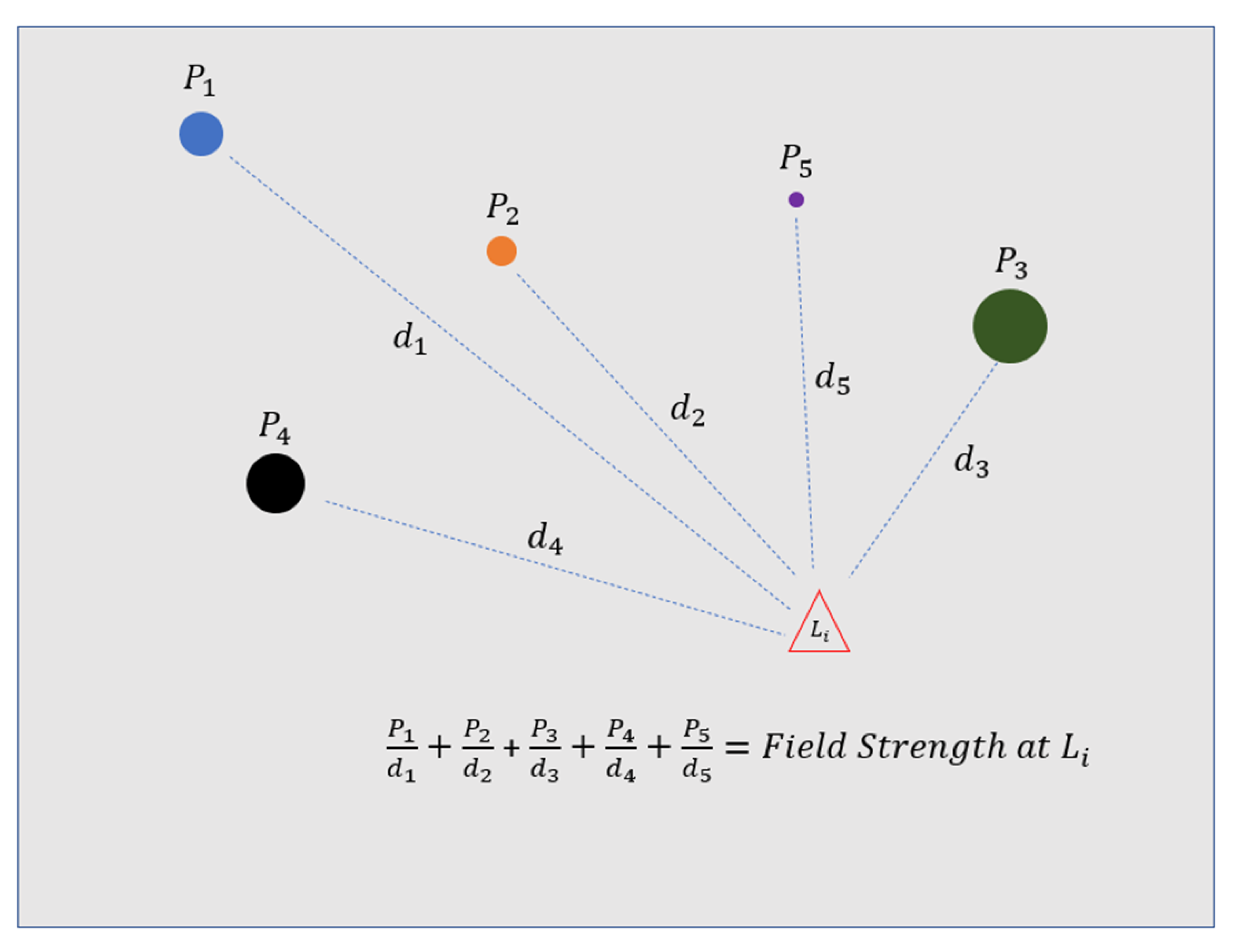
The idea of interacting spatial fields yields another result. The effect or “field strength” of phenomena at any location is the sum of all the spatial interactions. Figure 3 shows five instances of the same phenomenon, each at a different distance from a location of interest. The total effect at this location is the sum of their contributions.
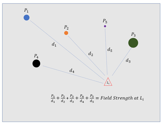
Figure 3.
Visualization of spatial interaction. Given phenomena 1–5, the strength of their effect, and their distance from location L, their collective impact at L is the sum of the values over their respective distances.
We approach vulnerability here as the degree to which change is likely to create adverse effects on the system [49]. Our concept of spatial relationships relies on positive spatial autocorrelation; the idea that, on average, proximal locations have more characteristics in common than those far apart, e.g., the system state at a randomly selected location 10 m away is going to be more similar than that of a randomly selected location 1000 km away [50]. IDW, as per Equation (1), expresses this concisely by attenuating the known values based on distance, in order to provide estimates.
It is for this reason that IDW is a ‘workhorse’ in spatial analysis when estimating phenomenon and feature values at locations for which no observation data are available, such as the amount of rainfall between rain collection gauges. It is computationally fast, easy to understand, and available in common geospatial analysis software packages (e.g., QGIS, ESRI products, etc.). It can be used in almost any conceivable problem involving location: pollution models, disease prevalence, precipitation and climatic variable estimates, genetic distribution, and habitat suitability are only a few possible applications [51,52,53,54,55].
2.3. Formalized Conception of PVI
Both the AWRVI and the ACCVI formalize their examination of community vulnerability as the product of system component interactions over time. We offer a spatially integrated version of community vulnerability as Equation (2), where is the vulnerability index score, and and are the researcher-chosen observations of risk, vulnerability, and/or resilience, and relevant geographic features, respectively.
is found as per Equation (3), below where is the min-max scaled value of observations in the community under evaluation and,
is the min-max scaled sum of the geographic feature scores (; themselves min-max scaled) divided by some power of the feature’s distance from the community, as per IDW (Equation (4)). An important distinction: the represents the total effect of the selected geographic features on the locations under study; it does not directly represent the effects of local permafrost changes on the geographic features. The spatial relationships between the system formed by the community and the geographic features underpin this subindex, and can be expressed succinctly as “more is not necessarily better”. To illustrate, dense, multiply-redundant, critical infrastructure located near a community is more likely to impact it, more often, than infrastructure further away. However, if the community is experiencing adverse effects from landscape changes, then the density of the infrastructure and its proximity cannot contribute to resilience or adaptability, and in fact is far more likely to create negative effect cascades.
As with AWRVI and the ACCVI, this formulation expresses community vulnerability as the product of the system components. In the first part of this study, we evaluated three classes of phenomena for their impact over space: infrastructure, the communities’ permafrost ranks from the Denali Commission Report, and the AWRVI assessments. In the second part, we applied the results to military locations to estimate their PVI and rank-order them accordingly.
2.4. Community Observation Selection
The Denali Commission and AWRVI study results were selected as observations that establish how changing permafrost is affecting communities. The Denali Commission Report community rankings constitute expert assessment of several data sources across nine community evaluation factors. Data used included remote and on-site observations, geo-technical reports, surface geology maps, terrain information, and scientific literature on permafrost distribution and behavior. The nine evaluation factors were the impacts to:
- Critical Infrastructure;
- Human Health and Safety;
- Subsistence and Shoreline Use;
- Land Use/Geograpic Location;
- Percentage of Population Affected;
- Housing Distribution;
- Environmental Threat;
- Cultural Importance;
- Commercial Infrastructure
The resulting rankings therefore include biophysical, sociocultural, and economic factors, as well as expert judgment (see ([36], pp. 4-4 to 4-14)). A rank of one indicated the highest permafrost threat score and 23 the lowest.
AWRVI was developed in 2008 to help communities examine their vulnerability to changing water resources, and was included in the Arctic Adaptation Exchange of the Arctic Council in 2018. AWRVI includes physical and social composite layers, and included temporal change, as well as the community perceptions of such changes. The objective was to enable communities to develop culturally and locationally specific strategies to adapt to and manage the availability of their water resources over time. The AWRVI was initially conducted with three Alaskan communities, then updated in 2018 based on participant feedback while being applied to four more Alaskan communities. AWRVI is comprised of physical and social sub-indices (Table 1). The results in each case were validated by community participants [28,30,31]. Using both the Denali Commission findings and the AWRVI study results incorporates a composite and integrative index into the PVI.

Table 1.
AWRVI Subindices.
2.5. Selection of Geographic Features
To select geographic features, we included inputs from security and defense practitioners and data from the long running Bering Sea Sub Network (BSSN) and the Community Observing Network for Adaptation and Security (CONAS), including changes to infrastructure resulting from permafrost thaw [56,57]. These networks consisted of Alaskan rural community residents, mainly Alaska Natives, who placed into context the consequences of infrastructure vulnerabilities and/or resilience taking place as the local environment changed [56,58]. Based on these diverse and extensive inputs we chose infrastructure that impacts not only the livelihoods and thrivability of arctic residents but also those which have connectivity to the continental United States. Impacts ranged from access to energy (i.e., crude oil, etc.), food resources, military and security systems that provide information and data required for defense and safety, transportation, including that at local community levels, minerals required for the functioning of a healthy national economy which provides the federal resources that are then returned back to arctic residents. We cordoned these into six categories of community-supporting infrastructure, which were then used to create the geographic feature sub-index: communications, transport, services, water, energy, and waste/pollution. A total of 22 infrastructure types, each with tens to thousands of publicly-available unique geographic features [59,60,61,62,63,64,65,66,67,68,69], were represented as per Table 2.
Table 2.
Infrastructure categories and types.
2.6. PVI Co-Design
Two levels of engagement were involved in the design and validation of the PVI. First, we leveraged the existing assessment of threats from permafrost thaw by the Denali Commission which was undertaken with input from Alaskan communities [35]—that is, a communities of people in specific locales (Figure 2). Second, the construction of the PVI equation and mapping utilized a quadrant-enabled Delphi (QED) approach [70] for eliciting and synthesizing input from federal, state, local, tribal, territorial, and private (FSLTTP) subject matter experts—representing a community of practice. The Denali Commission’s statewide threat assessment was undertaken by engineers from the U.S. Army Corps of Engineers, the U.S. Army Cold Regions Research and Engineering Laboratory, and the University of Alaska Fairbanks [35]. While no direct engagement with community members or community experts was conducted, the assessment did directly use the outcomes from the Alaska Baseline Erosion Survey that included a community survey of 127 respondents from 178 Alaskan communities who reported types and severity of erosion problems as well as the perceived success of corrective actions [35]. The PVI was co-developed with a diverse range of FSLTTP experts and representatives using the QED methodology [70]. A two-day virtual QED workshop was held 2–3 June 2020 to elicit and synthesize FSLTTP input. This involved 50 participants in three successive sessions organized in four quadrants to identify, rate, and rank components of risk, safety, security, and vulnerability in Arctic Alaska. By the final session on Day 2, a draft PVI and preliminary map outputs were presented and vetted.
2.7. PVI Construction
There were eight steps in PVI construction:
- Create quantitative scores for the 186 communities under study based on the Denali commission and AWRVI results;
- From these scores and the community locations, create an estimative raster surface over the study area for the Denali commission and AWRVI results (one for each) using IDW, which reflects the interactions of their systems over space (2 total raster surfaces);
- Aggregate the two rasters to obtain a single estimative surface representing ;
- Generate quantitative scores for each geographic feature within the 22 infrastructure types;
- Using these scores, calculate the effects of the geographic features on the communities under study using IDW;
- Generate one estimative raster surface for the effects of each of the 22 infrastructure types, as found in the preceding step (22 total raster surfaces);
- Aggregate the rasters from step six by category, then sum the six category rasters to create a single estimative surface representing ;
- Multiply these rasters element-wise to obtain a single raster representing the estimated PVI over the state of Alaska, and extract the values at the locations of the communities to obtain the community PVIs.
All calculations and spatial operations were done using a projected coordinate system and Euclidean distance. The details of implementation are discussed below.
2.7.1. Step 1: Scoring of Communities
The Denali Commission ranked each of the 186 communities into bins from 1 to 23, where 1 represented the communities most threatened by permafrost, and 23 those least threatened by permafrost. The AWRVI studies generated results between 1 and 0; a 1 would indicate the most vulnerable of communities, and 0 the least vulnerable. These are inverse schema: the lower value in the Denali Commission represents the greater threat, while a lower AWRVI value shows lower vulnerability. Scores were therefore assigned in the following manner. The reciprocal of the Denali Commission rank was used as the Denali Commission score, e.g., the rank of one remained one, while a reported rank of 18 generated a score of or 0.05556. The AWRVI results were directly used as the score. In this way, the scoring was matched; higher scores indicated greater threat or vulnerability, and lower scores lower threat or vulnerability.
2.7.2. Steps 2 and 3: Generating and Aggregating the Community Rasters
There were three considerations in generating the community rasters. First, the large difference between the Denali Commission and AWRVI sample size and distribution needed to be resolved. Secondly, the value for k in Equation (1) needed to demonstrate spatial interaction between the communities, while ensuring the raster’s estimate of the community score was accurate. Finally, the dissimilarity in scoring magnitudes had to be rectified.
The Denali Commission evaluated 186 remote communities (populations: min = 8, max = 6270, mean = 443, median = 245) in its permafrost rankings, resulting in Figure 4, while the AWRVI study evaluated 7, each of which was also part of the Denali Commission report. Using 7 unevenly distributed points to create an estimative surface over Alaska is infeasible. However, 179 Denali Commission communities did not have AWRVI scores. This was remedied by assigning the mean of the 7 AWRVI scores, 0.6257, to the the remaining communities. This ensured that all 186 community locations could be used in creating an AWRVI score estimative surface, without generating artificial minima and maxima in unobserved locations solely as a function of distance (Figure 5).
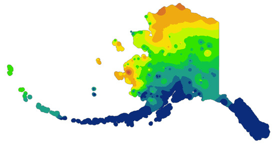
Figure 4.
An estimative raster surface generated from the 186 Denali Commission report scores. Cooler colors (blues and greens) indicate lower permafrost threat rankings, while hotter colors (yellows and reds) indicate higher rankings. See Figure 2 for community locations.
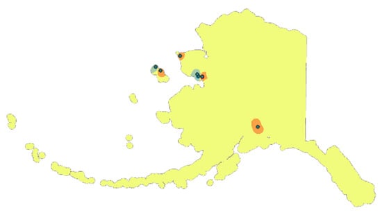
Figure 5.
An estimative raster surface generated from the AWRVI scores. Each color represents a different range of values. The study area is largely the same color, here yellow, indicating low variation (0.619–0.629 on a scale of 0–1, or ≈1%). The green points are the locations of communities included in the AWRVI studies.
When using IDW, the value of k in Equation (1) must be chosen to reflect how heavily the distance between two locations affects their interactions. As the equation suggests, higher values of k create rapid decreases in spatial interaction as the distance increases. This is seen, for example, in the inverse square laws of physics; e.g., gravity is as strong at twice the distance, rather than as strong. We chose a value of k, 1.75, to create the maximum spatial interaction between locations, while returning accurate estimates at observed locations, and preserving the community’s ordinal ranking based on its assigned Denali and AWRVI scores. Values of k below 1.75, representing stronger spatial interactions, created changes in ordinal rank, while values above 1.75 did not provide the maximum possible spatial interaction.
Both rasters were produced using the same extent boundaries and a cell size of 1000 m, to ensure an exact match between them, and prevent a need for resampling. The dissimilarity in scoring magnitudes between the rasters was solved through simple min-max scaling prior to their aggregation by summing. The raster cells all occupied the range with the lowest value scaled to 0 and the highest value scaled to 1. The resulting raster, representing , is presented in the section discussing step eight.
2.7.3. Step 4: Scoring the Geographic Features of Infrastructure Types
Where possible, the geographic features—some 15,000 in all—were scored according to an existing metric, e.g., capacity for fuel tanks, normal storage for dams, power line voltage, etc. In cases where no such metric existed, all features were treated as equivalent, and received a score of 1 (Table 3).
Table 3.
Infrastructure types and feature scoring.
2.7.4. Steps 5, 6, and 7: Calculating the Effects of Infrastructure on Communities Using IDW, Generating Estimative Rasters, and Aggregation to a Single Raster
The effect of each geographic feature (Figure 6) in the selected infrastructure types on all 186 communities evaluated in the Denali Commission report was calculated using Equation (4), with k again set to 1.75, for consistency. Each geographic feature within an infrastructure type therefore had 186 associated effect values. These were then summed to a single effect score, indicating how much that specific feature (e.g., an airport, dam, etc.) impacts the communities overall. These effect scores were then min–max scaled within type.
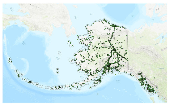
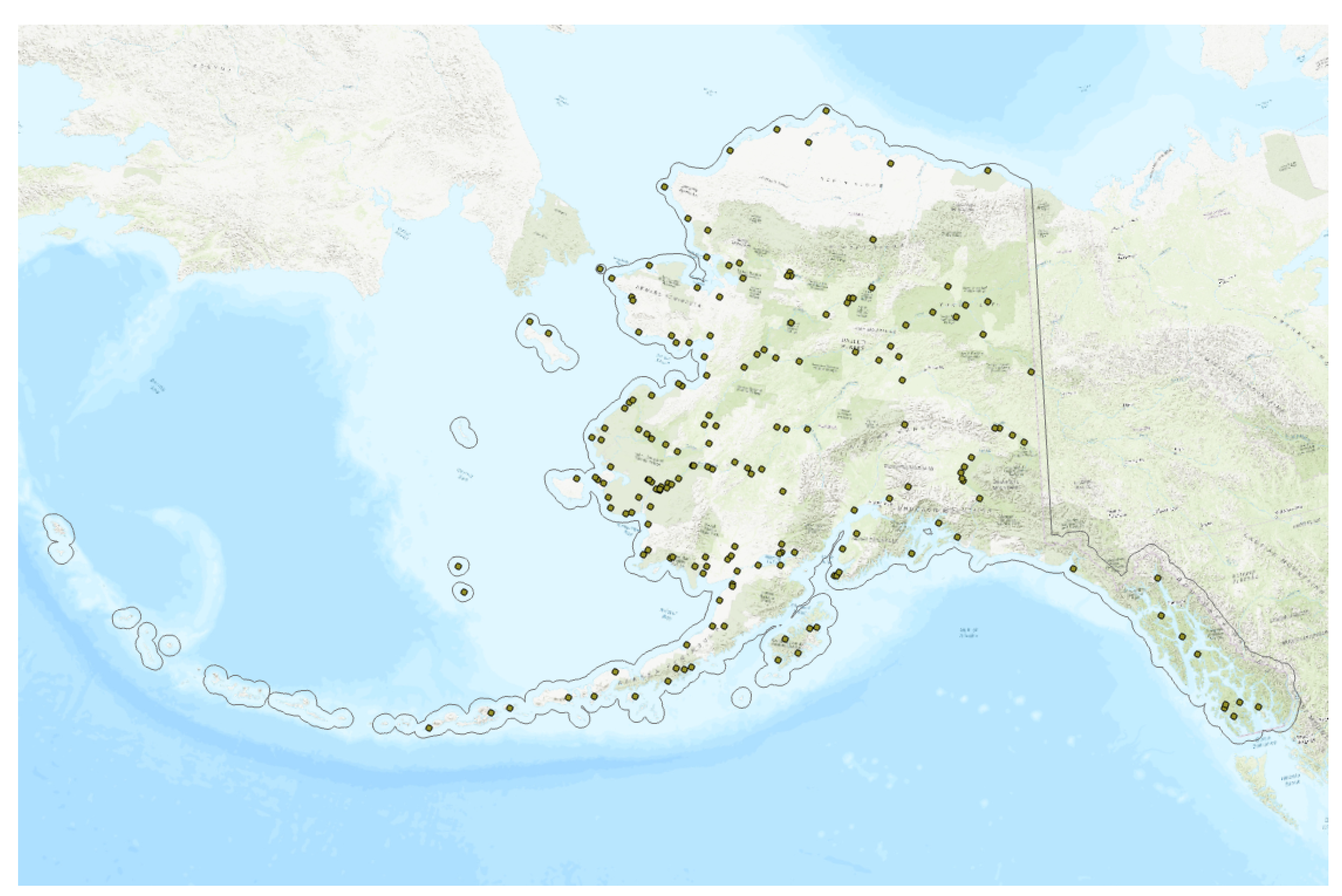
Figure 6.
Point locations of all geographic features as per Table 3, comprising the .
For features easily represented as points, this was a straightforward distance calculation between two sets of coordinates. However, three infrastructure types, power lines, roads, and the Trans-Alaska Pipeline System, are represented as line features. Here the line nearest each of the 186 communities was selected, and the point on that line closest to the community used in the calculation. This yielded a one-to-one mapping, such that these three infrastructure types were each spatially represented by their own set of 186 points. Calculations then proceeded as per the method used for point features.
Estimative raster surfaces of the infrastructure type effects on the communities were then generated using the same extent and cell size settings used in step two. An important point must be made here. During step two, the spatial interaction between the communities was directly calculated during raster creation i.e., k = 1.75. Here, k = 1.75 during the effects calculation using Equation (4). Consequently, direct linear interpolation was used to create the effects rasters; interpolating at a power of 1.75 would result in inappropriately applying the k value twice.
After this, the infrastructure type effect rasters were summed within their category. The resultant six category rasters were min–max scaled to account for the different number of types in each category and then summed into a single raster representing (Figure 7).
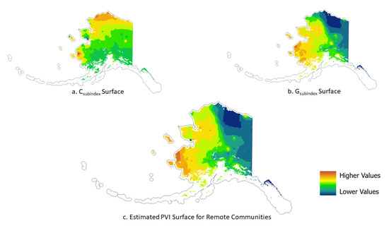
Figure 7.
(a) shows the estimated surface, (b) displays the surface, and (c) is the estimated PVI surface for the 186 Remote Communities that were evaluated by the Denali Commission Report. Cooler colors (blues and greens) represent locations with lower values, while hotter colors (yellow to red) are regions with higher values. White areas inside the Alaska outline are locations without permafrost.
2.7.5. Step 8: Creating the PVI Raster and Extracting the PVI for Each Community
The final step combined the and surfaces through element-wise (cell by cell) multiplication of their rasters. As summed two rasters, yielding possible values from [0, 2] while summed six rasters for values from [0, 6], min–max scaling was used a final time prior to multiplication, as per Equation (1). This raster was then clipped so its boundaries conformed to existing permafrost extent [71]; locations without permafrost are not directly vulnerable to the effects of permafrost thaw in their communities, nor is their surrounding infrastructure. We note this is reflected in the Denali Commission Report rankings—communities in these locations received the lowest rank (23). PVI values for the 186 communities were then extracted from the final raster (Figure 8).

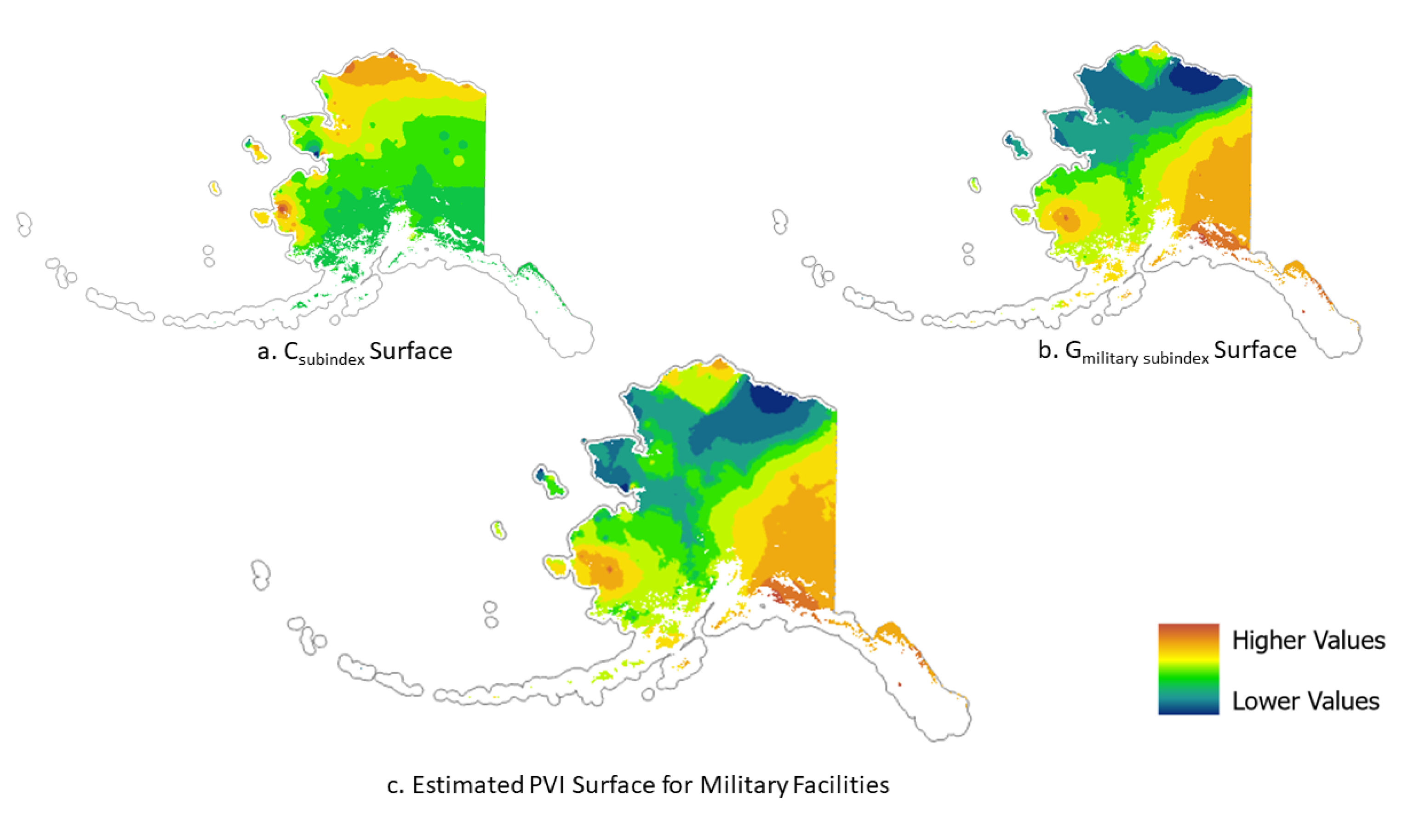
Figure 8.
(a) shows the estimated surface, (b) displays the surface, and (c) is the estimated PVI surface for the 30 military facilities. Cooler colors (blues and greens) represent locations with lower values, while hotter colors (yellow to red) are regions with higher values. White areas inside the Alaska outline are locations without permafrost.
2.8. PVI for Military Facilities
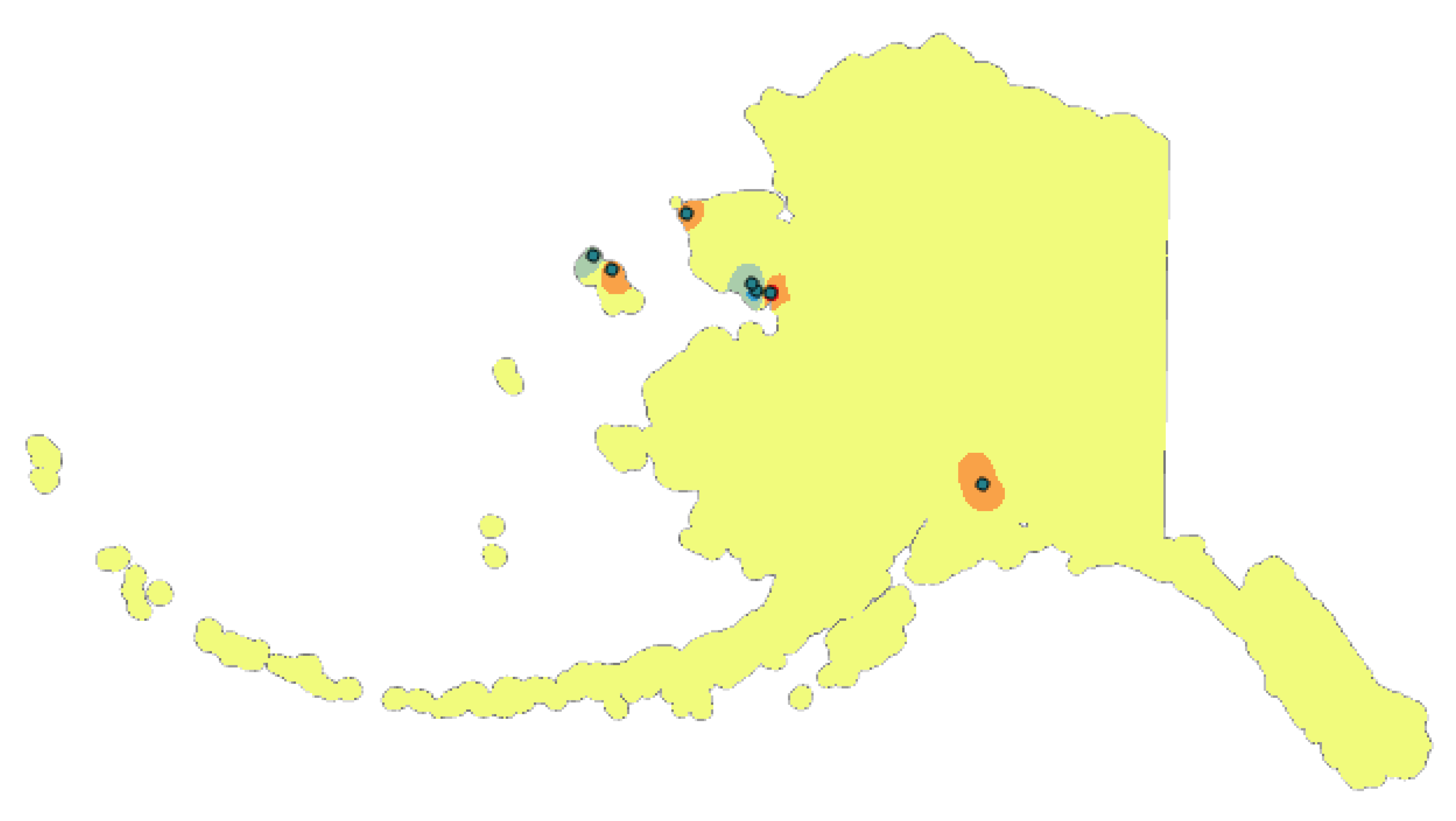
We applied the same eight steps to 30 military facilities in Alaska (Figure 9) to demonstrate versatility and how this spatial approach can be applied to fully non-observed locations. The surface was once again applied, but the spatial relationships of the infrastructure were recalculated into a based on their distances to the military facilities (Figure 8).
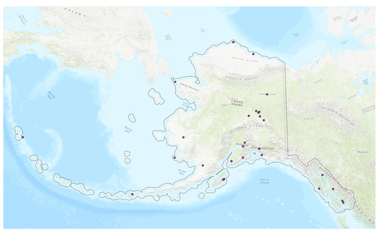
Figure 9.
Point locations of military facilities used to create Figure 8.
3. Results
The output maps (Figure 7 and Figure 8) met expectations for visual inspection; locations of higher and lower PVI are clearly delineated and easy to interpret, including initial vetting by experts and representatives at the QED workshop. The inclusion of state-wide, related infrastructure as part of the system evaluation had a clear effect on the spatial pattern; the (Figure 7a and Figure 8a) has obvious horizontal (east–west) banding, while the (Figure 7b and Figure 8b) show greater vertical orientation (north–south). This is reflected in the PVI surfaces (Figure 7c and Figure 8c). Visual tools are valuable communication devices for policy and decision makers (e.g., [16] etc.).
Mathematically, validation was approached by examining the statistical differences between the calculated and extracted values for all input locations for both sub-indices, as per Table 4. Unsurprisingly, the 15,000 geographic features comprising the infrastructure types showed the highest mean difference and standard deviation. However, even at = ±3, this amounts to only a ±0.094 error on a scale of [0, 1]. The accuracy of the estimative surface compared to directly calculated results is thus clearly within acceptable limits. As discussed in Section 2.7.2, the correlation between the Denali Commission permafrost threat rankings, and those derived from extracted values, was perfect, with .
Table 4.
Aggregate statistics for validating direct calculation vs. the values extracted from the estimative surfaces.
Our attention then turned to comparing PVI to an external metric; the permafrost threat index developed by the Denali Commission. We expected that since the AWRVI surface was fairly constant, the variation in the would be due mostly to the Denali Commission rankings. Since the is numerically of the PVI score, the correlation between the PVI values and the Denali Commission rankings should be about 0.5. This was borne out upon examination: we grouped the PVI results into the same number of ranks, and the same number of communities within each rank, as found in the Denali report, and established that . Values of that deviated substantially from this expectation would suggest the model was unreliable; the size and spatial distribution of the observations, and unit-distance between the ranks of the Denali study, made it a suitable baseline for comparison.
Digging deeper into the comparison shows that when using the PVI, 122 communities experienced some absolute change to their ranking, and 64 did not. A total of 14 showed statistically significant changes to their rankings at (. The greatest rank shift was experienced by the community of Togiak, which catapulted from 23 in the Denali Commission report to a rank of 2 using the PVI. This pointed to an exceptionally high value for the at that location, which proved correct—Togiak and its immediate vicinity had the second highest values in the data set. We provide the number of communities displaying statistically meaningful difference between their Denali Committee Report rankings and the PVI rankings, below (Table 5).
Table 5.
Number of communities showing statistically meaningful differences between their Denali Report Rankings and PVI scores.
4. Discussion
The initial PVI presented here provides decisional guidance even when the exact relationships between systems and subsystems have not yet been elucidated. The Denali Commission Report was careful to point out the uncertainties in their evaluation of threat from permafrost change (see Figures 5 and 6 in [36]) due to lack of data. Similarly, the PVI constructed here was conducted with sparse information about the exact relationships between the communities and state-wide infrastructure. More concretely establishing the importance of specific infrastructure systems ranging across Alaska to the individual communities would greatly improve the PVI value as a decision-making tool.
Nonetheless, the PVI is the first vulnerability index developed for permafrost and is a feasible initial method for calculating a field of effect for a phenomenon, feature, or event representing vulnerability, even when observations are sparse relative to the size of the study area. This delivers two-fold value. The low error in the interpolated surface when compared to the directly calculated values makes it a reliable visual and mathematical representation of what is known or assessed. As with any approach, the exact conception of distance relationships can be fine-tuned according to need, and the scoring/weighting methods for communities and infrastructure adjusted. Accuracy and precision of the estimative surfaces would improve with increased number and frequency of observations.
We emphasize that the PVI value at any point on the estimative surface represents the vulnerability of that location to the effects of changing permafrost, rather than representing the effects of permafrost change itself. To elucidate, consider a hypothetical community built on an island of stable geology, but surrounded by areas greatly affected by permafrost thaw. Regardless of its own geological stability, it remains vulnerable, systemically, to the effects of permafrost thaw in its surrounds. This is, in fact, the dynamic at play in Togiak’s rise from a rank of 23 in the Denali Commission Report to 2 in the PVI. While Togiak itself shows little impact from permafrost thaw effects, the region within a 250 km radius has 22 communities that show some effect. A total of 11 of these 22 communities are in the top 50% at-risk rankings according to the Denali Commission Report, while 8 are in the top one-third, and all of the infrastructure is close to their respective communities, accounting for the high score. Togiak’s dramatic shift in rank comes from its receipt of adverse cascade effects as part of a spatially interactive, community–community, community–landscape system.
On this basis, we offer that the PVI provides valuable insight for focused policy and decision making. One policy need, for instance, is the triage and prioritization of resources for mitigation to permafrost thaw. Here, the application of the PVI to military facilities, both Department of Defense and Department of Homeland Security, becomes relevant. These entities, like Alaskan communities, have a vested interest in long-term mitigation of vulnerabilities. The resources they bring include not only those which sustain existing infrastructure systems but also those which may be required to support the relocation and/or mitigation engineering of settlements underlain by thawing permafrost. These are costs that will fall to both the State of Alaska and the federal system. Finally, and perhaps most critically, in the mid- to longer-term permafrost thaw will severely impact ecosystems by changing the dynamics of sediment transport, surface and sub-surface freshwater balances, and near-shore habitats. The cascading effects of these changes are poorly understood yet have the ability to restructure entire ecosystems, which will change significantly, affecting the patterns of life and cultures of humans and other fauna. Assisting all potential partners in prioritization and decision making is therefore crucial as permafrost thaw continues.
At the moment, such decisions are limited to using past, or at best, present trends in the data. Further work could strive to achieve forecasting capabilities, which would enable policymakers to base their choices on reliably projected future scenarios. Agent-based modeling, the representation of real-world entities as simulated software agents, is one way to achieve these insightful projections. The application of agent-based modeling to understanding the future of the Arctic, especially as it pertains to permafrost degradation, is a topic of ongoing work [72]. There are also opportunities to combine agent-based capabilities with conceptions of distance and spatial interactions; these options should be further explored.
While the value of the PVI is to Alaska and the broader community of Arctic residents, what may be more important for other researchers is that the method used can incorporate additional indices, regardless of their own variables and sub-indices, to create an integrated risk, vulnerability, or resilience estimate for any location. This is particularly valuable when leveraging existing research, since most studies are limited both in geographic scope and spatial distribution within that scope. There are numerous risk-related indices, each with their own purpose and emphasis ranging from infrastructure to cultural practices (e.g., [16]). The spatial estimation presented in this paper provides a way to integrate any subset of them according to specific interests and needs. Similarly, IDW is not the only way to conceive of spatial relationships and derive an estimate. Far more advanced, but computationally intensive, methods exist and can be applied as warranted or preferred.
More specifically, the PVI is intended to be an interface between science and policy. In this context, the Denali Commission Report represented an important advancement in the collective understanding about how Alaskan communities—and presumably similar Arctic or near-Arctic communities worldwide—might be impacted by thawing permafrost. With the PVI, permafrost thaw is treated as a coupled social–ecological and technological system (SETS). The PVI provides an understanding of spatially explicit interactions with respect to permafrost vulnerability that enhances recent modeling toolbox efforts for permafrost landscapes [73]. The PVI is not advanced as an alternative to qualitative assessments to permafrost risk for Arctic communities but can compliment risk frameworks that are based on firsthand qualitative interactions (e.g., [74]) or fieldwork that encapsulates narratives of local realities of permafrost degradation [75]. Further advancements in the knowledge about how permafrost thaw and community adaptations to new physical conditions interact will come from a concerted systems science approach because SETS present interrelationships that should be considered when assessing hazard, threat, risk, vulnerability, and resilience. Doing this requires systematic assessments by teams of experts (e.g, using methods such as the QED), co-developed partnerships with communities, and regular field observations to understand how changes in one place or part of the system impact the others. The value of the PVI in this regard is that it identifies locations that may be of particular interest, and thus helps guide research and policy.
Author Contributions
Conceptualization, L.A. and J.V.; methodology, J.V. and L.A.; validation, L.A., S.M., C.M. and V.R.; formal analysis, J.V.; data curation, J.V.; writing—original draft preparation, L.A., J.V. and A.K.; writing—review and editing, L.A., J.V., A.K., S.M., C.M., S.H., V.R. and M.X.; visualization, J.V.; supervision, L.A. and A.K.; project administration, A.K.; funding acquisition, L.A., V.R. and M.X. All authors have read and agreed to the published version of the manuscript.
Funding
This research was funded by the U.S. National Science Foundation grant numbers ICER-1927713, ICER-1927708, and ICER-1927718.
Institutional Review Board Statement
The quadrant-enabled Delphi study was conducted according to the guidelines of the Declaration of Helsinki and under Chatham House rules, and approved by the Institutional Review Board of the University of Idaho (protocol code 18-084 approved on 26 April 2018 and protocol code 19-144 approved on 27 June 2019).
Informed Consent Statement
Informed consent was obtained from all quadrant-enabled Delphi workshop subjects involved in the study.
Data Availability Statement
Data available in publicly accessible repositories that do not issue DOIs. Publicly available datasets were analyzed in this study. These datasets are cited throughout the Methods section and can be found at the appropriate URLs included in the respective reference.
Acknowledgments
The authors are grateful to the local, tribal, territorial, state, and federal representatives for their individual and collective input on development of the PVI during the QED workshop.
Conflicts of Interest
The authors declare no conflict of interest.
Abbreviations
The following abbreviations are used in this manuscript:
| ACCI | Arctic Climate Change Index |
| AWRVI | Arctic Water Resources Vulnerability Index |
| HADR | Humanitarian Assistance and Disaster Response |
| IDW | Inverse Distance Weighting |
| PVI | Permafrost Vulnerability Index |
| SAR | Search and Rescue |
References
- National Research Council of Canada. Glossary of Permafrost and Related Ground-Ice Terms; Number 142 in Technical Memorandum; National Research Council: Ottawa, ON, Canada, 1988.
- Biskaborn, B.K.; Smith, S.L.; Noetzli, J.; Matthes, H.; Vieira, G.; Streletskiy, D.A.; Schoeneich, P.; Romanovsky, V.E.; Lewkowicz, A.G.; Abramov, A.; et al. Permafrost is warming at a global scale. Nat. Commun. 2019, 10, 264. [Google Scholar] [CrossRef] [PubMed]
- McKenzie, J.M.; Kurylyk, B.L.; Walvoord, M.A.; Bense, V.F.; Fortier, D.; Spence, C.; Grenier, C. Invited perspective: What lies beneath a changing Arctic? Cryosphere 2021, 15, 479–484. [Google Scholar] [CrossRef]
- Melnikov, V.P.; Osipov, V.I.; Brouchkov, A.V.; Falaleeva, A.A.; Badina, S.V.; Zheleznyak, M.N.; Sadurtdinov, M.R.; Ostrakov, N.A.; Drozdov, D.S.; Osokin, A.B.; et al. Climate warming and permafrost thaw in the Russian Arctic: Potential economic impacts on public infrastructure by 2050. Nat. Hazards 2022, 112, 231–251. [Google Scholar] [CrossRef]
- Hjort, J.; Karjalainen, O.; Aalto, J.; Westermann, S.; Romanovsky, V.E.; Nelson, F.E.; Etzelmüller, B.; Luoto, M. Degrading permafrost puts Arctic infrastructure at risk by mid-century. Nat. Commun. 2018, 9, 5147. [Google Scholar] [CrossRef] [PubMed]
- Lantz, T.C.; Kokelj, S.V. Increasing rates of retrogressive thaw slump activity in the Mackenzie Delta region, N.W.T., Canada. Geophys. Res. Lett. 2008, 35, L06502. [Google Scholar] [CrossRef]
- Lewkowicz, A.G.; Way, R.G. Extremes of summer climate trigger thousands of thermokarst landslides in a High Arctic environment. Nat. Commun. 2019, 10, 1329. [Google Scholar] [CrossRef]
- Hjort, J.; Streletskiy, D.; Doré, G.; Wu, Q.; Bjella, K.; Luoto, M. Impacts of permafrost degradation on infrastructure. Nat. Rev. Earth Environ. 2022, 3, 24–38. [Google Scholar] [CrossRef]
- Liew, M.; Xiao, M.; Farquharson, L.; Nicolsky, D.; Jensen, A.; Romanovsky, V.; Peirce, J.; Alessa, L.; McComb, C.; Zhang, X.; et al. Understanding Effects of Permafrost Degradation and Coastal Erosion on Civil Infrastructure in Arctic Coastal Villages: A Community Survey and Knowledge Co-Production. J. Mar. Sci. Eng. 2022, 10, 422. [Google Scholar] [CrossRef]
- Baltzer, J.L.; Veness, T.; Chasmer, L.E.; Sniderhan, A.E.; Quinton, W.L. Forests on thawing permafrost: Fragmentation, edge effects, and net forest loss. Glob. Chang. Biol. 2014, 20, 824–834. [Google Scholar] [CrossRef]
- Mamet, S.D.; Chun, K.P.; Kershaw, G.G.L.; Loranty, M.M.; Peter Kershaw, G. Recent Increases in Permafrost Thaw Rates and Areal Loss of Palsas in the Western Northwest Territories, Canada: Non-linear Palsa Degradation. Permafr. Periglac. Process. 2017, 28, 619–633. [Google Scholar] [CrossRef]
- Mann, P.J.; Strauss, J.; Palmtag, J.; Dowdy, K.; Ogneva, O.; Fuchs, M.; Bedington, M.; Torres, R.; Polimene, L.; Overduin, P.; et al. Degrading permafrost river catchments and their impact on Arctic Ocean nearshore processes. Ambio 2022, 51, 439–455. [Google Scholar] [CrossRef] [PubMed]
- Gartler, S.; Larsen, J.N.; Ingimundarson, J.H.; Schweitzer, P.; Povoroznyuk, O.; Meyer, A. A Risk Analysis Framework: Key Risks from Permafrost Thaw in Arctic Coastal Areas. 2022. Available online: https://ui.adsabs.harvard.edu/abs/2022EGUGA..24.7937G/abstract (accessed on 18 August 2023).
- Kahn, S. It Takes a Village: Repurposing Takings Doctrine to Address Melting Permafrost in Alaska Native Towns. Alsk. Law Rev. 2022, 39, 105–138. [Google Scholar]
- Timlin, U.; Meyer, A.; Nordström, T.; Rautio, A. Permafrost thaw challenges and life in Svalbard. Curr. Res. Environ. Sustain. 2022, 4, 100122. [Google Scholar] [CrossRef]
- Beccari, B. A Comparative Analysis of Disaster Risk, Vulnerability and Resilience Composite Indicators. PLoS Curr. 2016, 8, ecurrents. [Google Scholar] [CrossRef] [PubMed]
- Walvoord, M.A.; Striegl, R.G. Complex Vulnerabilities of the Water and Aquatic Carbon Cycles to Permafrost Thaw. Front. Clim. 2021, 3, 730402. [Google Scholar] [CrossRef]
- Wolken, G.J.; Liljedahl, A.K.; Brubaker, M.; Coe, J.A.; Fiske, G.; Christiansen, H.H.; Jacquemart, M.; Jones, B.M.; Kääb, A.; Løvholt, F.; et al. Glacier and Permafrost Hazards. Arctic Rep. Card 2021, 21, 13. [Google Scholar] [CrossRef]
- Versen, J.; Mnatsakanyan, Z.; Urpelainen, J. Concerns of climate intervention: Understanding geoengineering security concerns in the Arctic and beyond. Clim. Chang. 2022, 171, 27. [Google Scholar] [CrossRef]
- Chalecki, E.L. He who would rule: Climate change in the Arctic and its implications for U.S. national security. J. Public Int. Aff. 2007, 18, 204–222. [Google Scholar]
- Strawa, A.W.; Latshaw, G.; Farkas, S.; Russell, P.; Zornetzer, S. Arctic Ice Loss Threatens National Security: A Path Forward. Orbis 2020, 64, 622–636. [Google Scholar] [CrossRef]
- Åtland, K. The Security Implications of Climate Change in the Arctic Ocean. In Environmental Security in the Arctic Ocean; Berkman, P.A., Vylegzhanin, A.N., Eds.; NATO Science for Peace and Security Series C: Environmental Security; Springer: Dordrecht, The Netherlands, 2013; pp. 205–216. [Google Scholar] [CrossRef]
- Crépin, A.S.; Karcher, M.; Gascard, J.C. Arctic Climate Change, Economy and Society (ACCESS): Integrated perspectives. Ambio 2017, 46, 341–354. [Google Scholar] [CrossRef]
- Kraska, J. Arctic Security in an Age of Climate Change; Cambridge University Press: Cambridge, UK, 2011. [Google Scholar]
- Ritchie, M.; Frazier, T.; Johansen, H.; Wood, E. Early climate change indicators in the Arctic: A geographical perspective. Appl. Geogr. 2021, 135, 102562. [Google Scholar] [CrossRef]
- Box, J.E.; Colgan, W.T.; Christensen, T.R.; Schmidt, N.M.; Lund, M.; Parmentier, F.J.W.; Brown, R.; Bhatt, U.S.; Euskirchen, E.S.; Romanovsky, V.E.; et al. Key indicators of Arctic climate change: 1971–2017. Environ. Res. Lett. 2019, 14, 045010. [Google Scholar] [CrossRef]
- Dogulu, N.; Karagiannis, G.M.; Synolakis, C.E.; Yalciner, A.; Necmioglu, O.; Sozdinler, C.O. Report on Institutional Plans, Operative Response Capacities and Needs for Crisis Management and Capacity Building. 2016. [Google Scholar] [CrossRef]
- Alessa, L.; Kliskey, A.; Lammers, R.; Arp, C.; White, D.; Hinzman, L.; Busey, R. The Arctic Water Resource Vulnerability Index: An Integrated Assessment Tool for Community Resilience and Vulnerability with Respect to Freshwater. Environ. Manag. 2008, 42, 523. [Google Scholar] [CrossRef] [PubMed]
- Debortoli, N.S.; Clark, D.G.; Ford, J.D.; Sayles, J.S.; Diaconescu, E.P. An integrative climate change vulnerability index for Arctic aviation and marine transportation. Nat. Commun. 2019, 10, 2596. [Google Scholar] [CrossRef] [PubMed]
- Kliskey, A.; Williams, P.; Abatzoglou, J.T.; Alessa, L.; Lammers, R.B. Enhancing a community-based water resource tool for assessing environmental change: The arctic water resources vulnerability index revisited. Environ. Syst. Decis. 2019, 39, 183–197. [Google Scholar] [CrossRef]
- Spence, C.; Norris, M.; Bickerton, G.; Bonsal, B.; Brua, R.; Culp, J.; Dibike, Y.; Gruber, S.; Morse, P.; Peters, D.; et al. The Canadian Water Resource Vulnerability Index to Permafrost Thaw (CWRVIPT). Arct. Sci. 2020, 6, 437–462. [Google Scholar] [CrossRef]
- Reidmiller, D.R.; Avery, C.W.; Easterling, D.R.; Kunkel, K.E.; Lewis, K.L.; Maycock, T.K.; Stewart, B.C. Impacts, Risks, and Adaptation in the United States: The Fourth National Climate Assessment, Volume II; Technical Report; U.S. Global Change Research Program: Washington, DC, USA, 2018. [Google Scholar] [CrossRef]
- Field, C.B. Intergovernmental Panel on Climate Change.( Eds.) Managing the Risks of Extreme Events and Disasters to Advance Climate Change Adaption: Special Report of the Intergovernmental Panel on Climate Change; Cambridge University Press: New York, NY, USA, 2012. [Google Scholar]
- Nevalainen, M.; Vanhatalo, J.; Helle, I. Index-based approach for estimating vulnerability of Arctic biota to oil spills. Ecosphere 2019, 10, e02766. [Google Scholar] [CrossRef]
- United States Congress. Denali Commission Act 1998; United States Congress: Washington, DC, USA, 1998; Section: 3121.
- University of Alaska, Fairbanks Institute of Northern Engineering; U.S. Army Corps of Engineers Alaska District; U.S. Army Corps of Engineers Cold Regions Research and Engineering Laboratory. Statewide Threat Assessment: Identification of Threats from Erosion, Flooding, and Thawing Permafrost in Remote Alaska Communities; Denali Commission: Anchorage, AK, USA, 2019.
- Aven, T. On Some Recent Definitions and Analysis Frameworks for Risk, Vulnerability, and Resilience. Risk Anal. 2011, 31, 515–522. [Google Scholar] [CrossRef]
- Kovaleva, O.; Sergeev, A.; Ryabchuk, D. Coastal vulnerability index as a tool for current state assessment and anthropogenic activity planning for the Eastern Gulf of Finland coastal zone (the Baltic Sea). Appl. Geogr. 2022, 143, 102710. [Google Scholar] [CrossRef]
- Johnson, D.P.; Stanforth, A.; Lulla, V.; Luber, G. Developing an applied extreme heat vulnerability index utilizing socioeconomic and environmental data. Appl. Geogr. 2012, 35, 23–31. [Google Scholar] [CrossRef]
- Harvey, D.W. Pattern, Process, and the Scale Problem in Geographical Research. Trans. Inst. Br. Geogr. 1968, 45, 71–78. [Google Scholar] [CrossRef]
- Tobler, W. A Computer Movie Simulating Urban Growth in the Detroit Region. Econ. Geogr. 1970, 46, 234–240. [Google Scholar] [CrossRef]
- Tobler, W. On the First Law of Geography: A Reply. Ann. Assoc. Am. Geogr. 2004, 94, 304–310. [Google Scholar] [CrossRef]
- Foresman, T.; Luscombe, R. The second law of geography for a spatially enabled economy. Int. J. Digit. Earth 2017, 10, 979–995. [Google Scholar] [CrossRef]
- Anderson, J.E. The Gravity Model. Annu. Rev. Econ. 2011, 3, 133–160. [Google Scholar] [CrossRef]
- Poot, J.; Alimi, O.; Cameron, M.P.; Maré, D.C. The Gravity Model of Migration: The Successful Comeback of an Ageing Superstar in Regional Science. J. Reg. Res. 2016, 36, 63–86. [Google Scholar] [CrossRef]
- Zipf, G.K. The P1 P2/D Hypothesis: On the Intercity Movement of Persons. Am. Sociol. Rev. 1946, 11, 677–686. [Google Scholar] [CrossRef]
- Boulding, K. Conflict and Defense: A General Theory; Harper & Row: New York, NY, USA, 1962. [Google Scholar]
- Haynes, K.; Fotheringham, A. Gravity and Spatial Interaction Models; WVU Regional Research Repository, West Virginia University: Morgantown, WV, USA, 2020; Available online: https://researchrepository.wvu.edu/rri-web-book/16/ (accessed on 18 August 2023).
- Naylor, A.; Ford, J.; Pearce, T.; Van Alstine, J. Conceptualizing Climate Vulnerability in Complex Adaptive Systems. ONE Earth 2020, 2, 444–454. [Google Scholar] [CrossRef]
- Haining, R. Spatial Sampling. In International Encyclopedia of the Social & Behavioral Sciences; Elsevier: Amsterdam, The Netherlands, 2001; pp. 14822–14827. [Google Scholar] [CrossRef]
- Blanco, I.; de Serres, F.J.; Cárcaba, V.; Lara, B.; Fernández-Bustillo, E. Alpha-1 Antitrypsin Deficiency PI*Z and PI*S Gene Frequency Distribution Using on Maps of the World by an Inverse Distance Weighting (IDW) Multivariate Interpolation Method. Hepat. Mon. 2012, 12, e7434. [Google Scholar] [CrossRef]
- Blanco, I.; Diego, I.; Bueno, P.; Fernández, E.; Casas-Maldonado, F.; Esquinas, C.; Soriano, J.B.; Miravitlles, M. Geographical distribution of COPD prevalence in Europe, estimated by an inverse distance weighting interpolation technique. Int. J. Chronic Obstr. Pulm. Dis. 2017, 13, 57–67. [Google Scholar] [CrossRef]
- Chen, F.W.; Liu, C.W. Estimation of the spatial rainfall distribution using inverse distance weighting (IDW) in the middle of Taiwan. Paddy Water Environ. 2012, 10, 209–222. [Google Scholar] [CrossRef]
- Ozelkan, E.; Bagis, S.; Ozelkan, E.C.; Ustundag, B.B.; Yucel, M.; Ormeci, C. Spatial interpolation of climatic variables using land surface temperature and modified inverse distance weighting. Int. J. Remote Sens. 2015, 36, 1000–1025. [Google Scholar] [CrossRef]
- Varatharajan, R.; Manogaran, G.; Priyan, M.K.; Balaş, V.E.; Barna, C. Visual analysis of geospatial habitat suitability model based on inverse distance weighting with paired comparison analysis. Multimed. Tools Appl. 2018, 77, 17573–17593. [Google Scholar] [CrossRef]
- Alessa, L.; Beaujean, G.; Bower, L.; Campbell, I.; Chemenko, O.; Copchiak, M.; Fidel, M.; Fleener, U.; Gamble, J.; Gundersen, A.; et al. Bering Sea Sub-Network II: Sharing Knowledge, Improving Understanding, Enabling Response; International community-based environmental observation alliance for a changing Arctic; Technical Report; Conservation of Arctic Flora and Fauna: Akureyri, Iceland, 2015. [Google Scholar]
- Cochran, P.; Huntington, O.H.; Pungowiyi, C.; Tom, S.; Chapin, F.S.; Huntington, H.P.; Maynard, N.G.; Trainor, S.F. Indigenous frameworks for observing and responding to climate change in Alaska. In Climate Change and Indigenous Peoples in the United States; Maldonado, J.K., Colombi, B., Pandya, R., Eds.; Springer International Publishing: Cham, Switzerland, 2013; pp. 49–59. [Google Scholar] [CrossRef]
- Alessa, L.; Williams, P.; Kliskey, A.; Beaujean, G. Incorporating Community-based Observing Networks and Systems: Toward a Regional Early Warning System for Enhanced Response to Arctic Critical Events. Wash. J. Environ. Law Policy 2016, 6, 1–27. [Google Scholar]
- Alaska Department of Transportation and Public Facilities. Transportation Geographic Information Section: DOT&PF Management Responsibility; State of Alaska: Juneau, AK, USA, 2018.
- Alaska Department of Transportation and Public Facilities. Transportation Geographic Information Section: Alaska’s Public Airports in Alaska; State of Alaska: Juneau, AK, USA, 2018.
- Alaska Energy Authority. State of Alaska Open Data Geoportal: Bulk Fuel Facilities; State of Alaska: Juneau, AK, USA, 2020.
- Alaska Energy Authority, TAPS. State of Alaska Open Data Geoportal: TAPS; State of Alaska: Juneau, AK, USA, 2020.
- Alaska Department of Public Safety. State of Alaska Open Data Geoportal: State Patrol Locations; State of Alaska: Juneau, AK, USA, 2020.
- Alaska Department of Transportation and Public Facilities. Transportation Geographic Information Section: Alaska’s Harbor System; State of Alaska: Juneau, AK, USA, 2018.
- Alaska Department of Transportation and Public Facilities. Transportation Geographic Information Section: Ferry Terminals in Alaska; State of Alaska: Juneau, AK, USA, 2018.
- Alaska Department of Commerce, Community, and Economic Development. State of Alaska Open Data Geoportal: Energy Transmission Lines; State of Alaska: Juneau, AK, USA, 2020.
- Alaska Department of Commerce, Harbors and Docks. State of Alaska Open Data Geoportal: Harbors and Docks; State of Alaska: Juneau, AK, USA, 2021.
- Alaska Department of Environmental Conservation, Division of Water. Alaska Open Data Geoportal: Water Distribution; State of Alaska: Juneau, AK, USA, 2021.
- Alaska Department of Environmental Conservation, LUST. State of Alaska Open Data Geoportal: Contaminated Sites; State of Alaska: Juneau, AK, USA, 2021.
- Alessa, L.; Moon, S.; Griffith, D.; Kliskey, A. Operator Driven Policy: Deriving Action From Data Using The Quadrant Enabled Delphi (QED) Method. Homel. Secur. Aff. 2018, 14. Available online: https://www.hsaj.org/articles/145866 (accessed on 18 August 2023).
- Obu, J.; Westermann, S.; Bartsch, A.; Berdnikov, N.; Christiansen, H.H.; Dashtseren, A.; Delaloye, R.; Elberling, B.; Etzelmüller, B.; Kholodov, A.; et al. Northern Hemisphere permafrost map based on TTOP modelling for 2000–2016 at 1 km2 scale. Earth-Sci. Rev. 2019, 193, 299–316. [Google Scholar] [CrossRef]
- Hicks, S.; Alessa, L.; McComb, C. Agents and the Arctic: The Case for Increased Use of Agent-Based Modeling to Study Permafrost; Contribution of the Arctic Institute: Washington, DC, USA, 2021. Available online: https://par.nsf.gov/servlets/purl/10289556 (accessed on 18 August 2023).
- Overeem, I.; Jafarov, E.; Wang, K.; Schaefer, K.; Stewart, S.; Clow, G.; Piper, M.; Elshorbany, Y. A Modeling Toolbox for Permafrost Landscapes. Eos Trans. Am. Geophys. Union (Online) 2018, 99. [Google Scholar] [CrossRef]
- Larsen, J.N.; Schweitzer, P.; Abass, K.; Doloisio, N.; Gartler, S.; Ingeman-Nielsen, T.; Ingimundarson, J.H.; Jungsberg, L.; Meyer, A.; Rautio, A.; et al. Thawing Permafrost in Arctic Coastal Communities: A Framework for Studying Risks from Climate Change. Sustainability 2021, 13, 2651. [Google Scholar] [CrossRef]
- Ulturgasheva, O.; Bodenhorn, B. (Eds.) Risky Futures: Climate, Geopolitics and Local Realities in the Uncertain Circumpolar North, 1st ed.; Berghahn Books: New York, NY, USA, 2022. [Google Scholar] [CrossRef]


Disclaimer/Publisher’s Note: The statements, opinions and data contained in all publications are solely those of the individual author(s) and contributor(s) and not of MDPI and/or the editor(s). MDPI and/or the editor(s) disclaim responsibility for any injury to people or property resulting from any ideas, methods, instructions or products referred to in the content. |
© 2023 by the authors. Licensee MDPI, Basel, Switzerland. This article is an open access article distributed under the terms and conditions of the Creative Commons Attribution (CC BY) license (https://creativecommons.org/licenses/by/4.0/).