Biomechanical Modeling and Simulation of the Knee Joint: Integration of AnyBody and Abaqus

Abstract

Background: The knee joint performs a vital function in human movement, supporting significant loads and ensuring stability during daily activities. Methods: The objective of this study was to develop and validate a subject-specific framework to model knee flexion–extension by integrating 3D gait data with individualized musculoskeletal (MS) and finite element (FE) models. In this proof of concept, gait data were collected from a 52-year-old woman using Xsens inertial sensors. The MS model was based on the same subject to define realistic loading, while the 3D knee FE model, built from another individual’s MRI, included all major anatomical structures, as subject-specific morphing was not possible due to unavailable scans. Results: The FE simulation showed principal stresses from –28.67 to +44.95 MPa, with compressive stresses between 2 and 8 MPa predominating in the tibial plateaus, consistent with normal gait. In the ACL, peak stress of 1.45 MPa occurred near the femoral insertion, decreasing non-uniformly with a compressive dip around –3.0 MPa. Displacement reached 0.99 mm in the distal tibia and decreased proximally. ACL displacement ranged from 0.45 to 0.80 mm, following a non-linear pattern likely due to ligament geometry and local constraints. Conclusions: These results support the model’s ability to replicate realistic, patient-specific joint mechanics.

1. Introduction

The knee is one of the most important joints in the human musculoskeletal system, performing a crucial role in locomotion and body stability. However, due to its structural and functional complexity, the knee is particularly susceptible to injuries and degenerative processes, which represent significant challenges for public health and advancements in orthopedic rehabilitation [1]. To better understand the mechanics underlying such conditions, the integration of musculoskeletal (MS) models and finite element (FE) models has proven to be a powerful approach [2,3]. This combined modeling enables a detailed analysis of the interactions between muscles, bones, and ligaments, offering a comprehensive understanding of joint function and load distribution critical for advancing injury treatment and rehabilitation strategies. While laboratory-based motion capture systems remain the gold standard for biomechanical assessment, their high cost and limited accessibility restrict widespread clinical adoption [4,5]. Although portable sensors, such as wearables and cameras, are affected by soft-tissue artifacts and muscle-induced motion noise, they remain promising alternatives for evaluating ACL injury risk and monitoring rehabilitation progress [6,7]. Despite the fact that previous studies have applied this methodology to populations with knee osteoarthritis [8] or in specific structures such as the tibia [9], its application to post-operative conditions, such as anterior cruciate ligament (ACL) reconstruction, remains limited [10,11].

A key component of performing biomechanical analyses is the accurate capture and modeling of human movement. Technologies such as Xsens MVN Analyze, based on inertial measurement units (IMUs), enable 3D motion tracking during gait [12]. Complementing motion capture, platforms like the AnyBody Modeling System provide subject-specific musculoskeletal modeling and simulation, enabling the estimation of internal forces such as muscle forces and joint loads [13]. While kinematics describes motion without accounting for forces, kinetics focuses on the internal and external forces acting on the body, including ground reaction forces and muscle forces. A comprehensive biomechanical analysis requires the integration of both kinematic and kinetic perspectives to fully characterize joint dynamics.

The integration of Xsens MVN Analyze with the AnyBody Modeling System allows motion capture data to be directly incorporated into subject-specific musculoskeletal models, enabling the estimation of muscle forces and joint loads throughout the gait cycle. Subsequently, the outputs from AnyBody, such as joint angles and reaction forces, can be transferred to FE software like Abaqus (Dassault Systèmes) to perform detailed biomechanical simulations [14]. This connection enables the evaluation of stress and strain distributions in biological tissues under physiologically relevant loading conditions, bridging the gap between movement analysis and tissue-level mechanics.

This study introduces a novel, fully integrated, patient-specific modeling pipeline that seamlessly incorporates gait acquisition data into FE simulations, specifically tailored for individuals who have undergone ACL reconstruction. By individualizing the modeling approach, this study aims to provide a more accurate and clinically relevant understanding of post-operative knee mechanics.

2. Methods

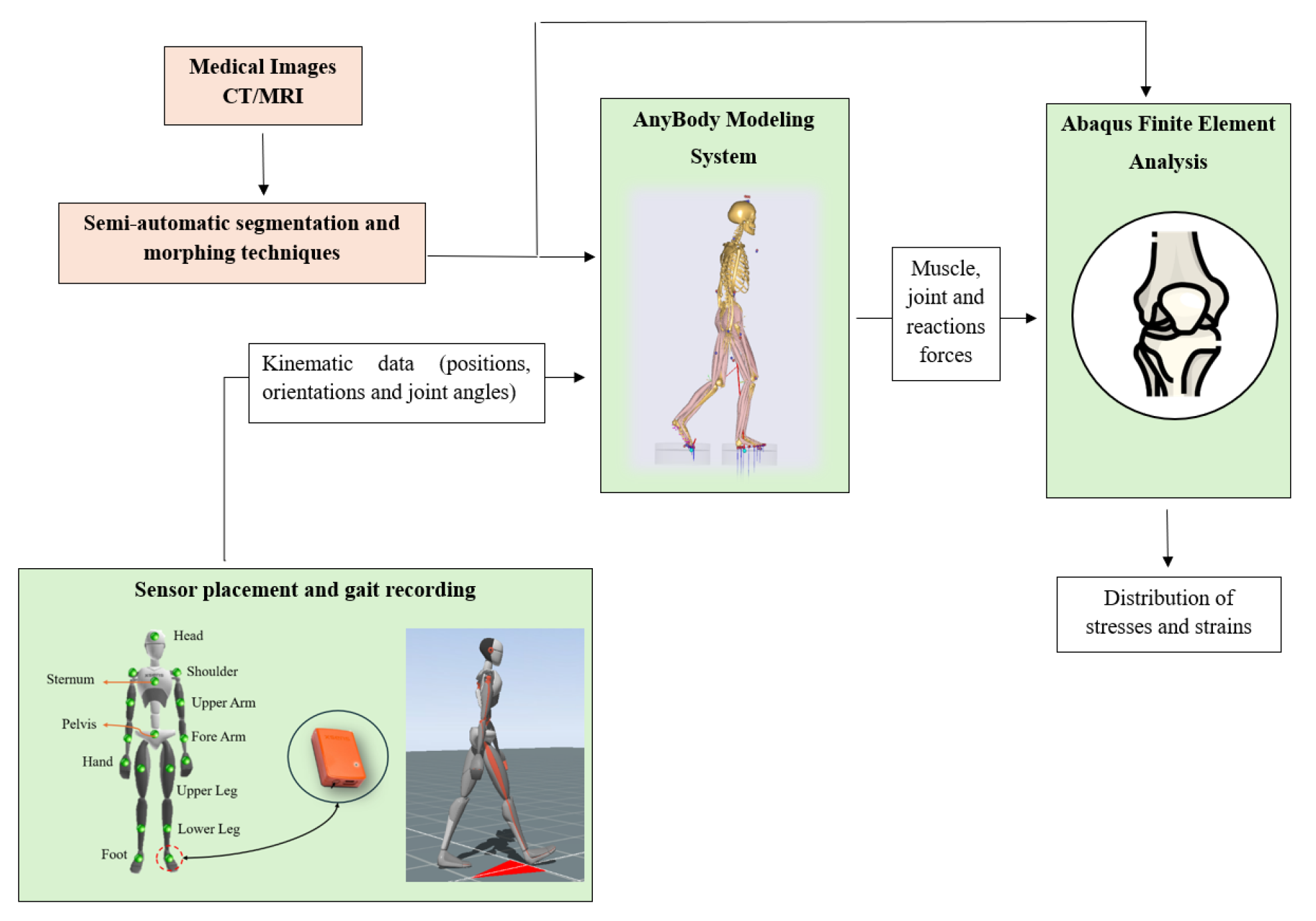
2.1. Workflow and Subject Information

This work presents an implementation of a biomechanical simulation workflow that integrates motion capture with MS and FE modeling. While anatomical personalization is still being refined, the current stage demonstrates the feasibility of combining real gait data with stress analysis at the knee joint. The full workflow is illustrated in Figure 1, which highlights the future integration of patient-specific imaging through morphing techniques.

As a proof-of-concept, one female subject (52 years old, 79 kg, 1.69 m) with a history of ACL reconstruction on the right knee participated in the experimental data collection. The Body Mass Index (BMI) was calculated as 27.7 kg/m², classifying the subject as overweight according to the World Health Organization (WHO).

Functional evaluation of the subject was conducted using two standardized outcome measures: the Knee Injury and Osteoarthritis Outcome Score (KOOS) and the International Knee Documentation Committee (IKDC) subjective knee evaluation form. These tools were used to assess knee function, pain, and quality of life after ACL reconstruction.

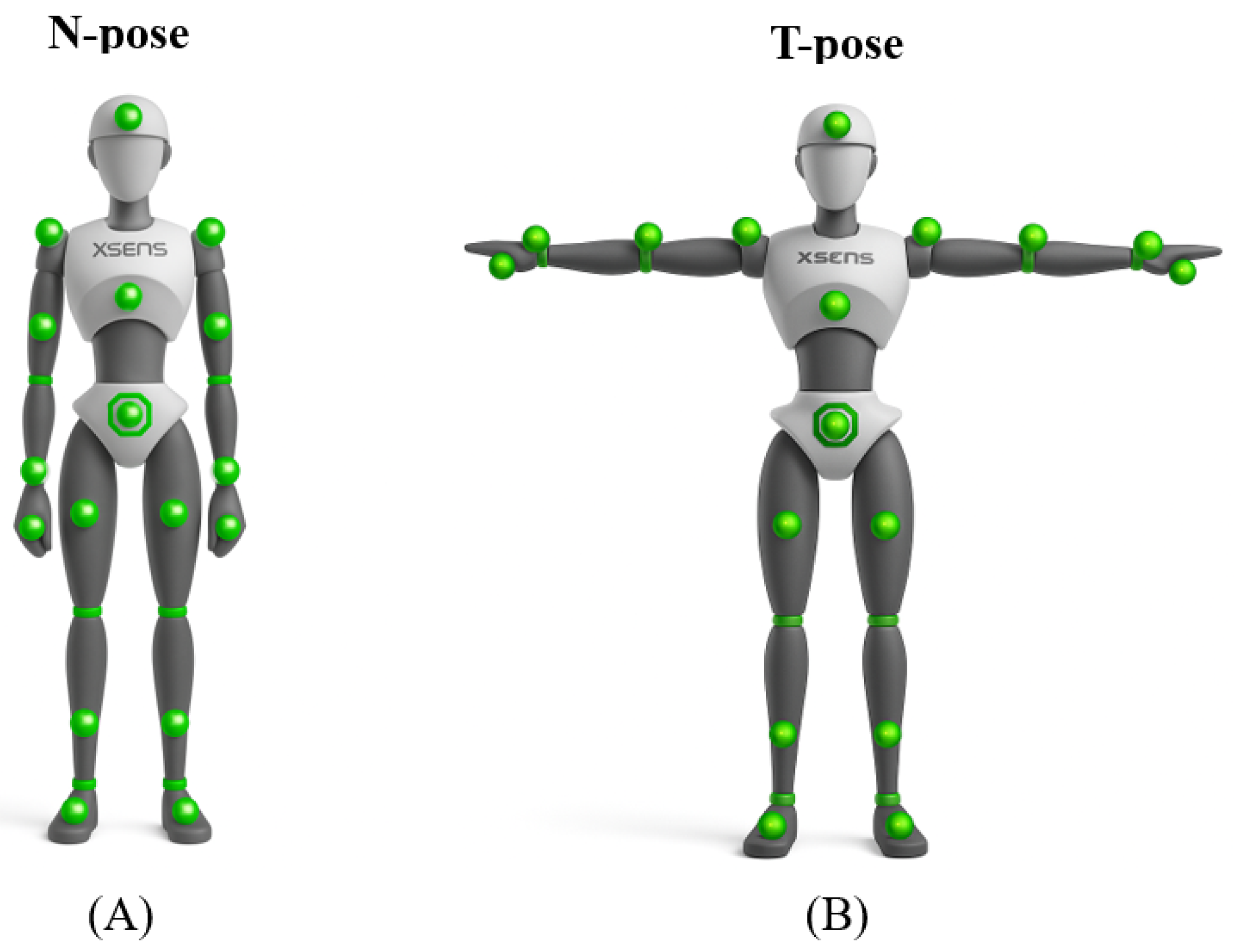
2.2. Data Collection

Xsens is a motion-capture platform composed of both hardware and software components, which are described below:

(1) Xsens MVN Hardware: is available as a body-wired solution that streams data wirelessly to a laptop (MVN Link). It consists of multiple wired motion trackers (MTx) connected to an on-body data hub (BodyPack), which provides both power and data aggregation. A custom lycra suit with dedicated zippers simplifies the placement of the trackers at specific anatomical landmarks. Seventeen motion trackers are mounted on the feet, lower legs, upper legs, pelvis, shoulders, sternum, head, upper arms, forearms, and hands to capture full-body motion. Each tracker integrates a 3D gyroscope, accelerometer, and magnetometer. An advanced onboard signal-processing pipeline, incorporating patented StrapDown Integration (SDI) algorithms, fuses raw sensor data sampled at high internal rates (>1 kHz) and outputs stable, drift-free motion data up to 240 Hz when higher update rates are required.

(2) Xsens MVN Software: to ensure accurate analysis, it is necessary to perform reprocessing in high definition (HD) within the software. The Single Level scenario was selected, given that the subject was walking on a flat, level surface.

In terms of experimental protocol, the data collection followed the guidelines provided by the Xsens MVN Analyze software for gait analysis, ensuring standardized procedures and reliable data acquisition. Initially, body measurements were collected to be input into the Xsens system, allowing for accurate initialization of the subject-specific motion capture model, as shown in

Table 1. Body measurements collected for Xsens model initialization.

Measurement	Value (cm)
Body Height	169.00
Foot or Shoe Length	25.00
Shoulder Height	147.86
Shoulder Width	37.98
Elbow Span	94.20
Wrist Span	143.39
Arm Span	180.14
Hip Height	88.00
Hip Width	28.00
Ankle Height	8.00
Extra Shoe Sole Thickness	0.00

.

Then, a sensor-to-segment calibration procedure was performed to align the motion capture system with the subject’s anatomical structure. This calibration involved asking the participant to assume a known static pose (e.g., N-pose or T-pose in Figure 2), while sensor orientations were estimated by combining accelerometer readings (for inclination) and magnetometer readings (for heading). The calibration was performed using the N-pose, where the participant stood upright with arms relaxed alongside the body and thumbs pointing forward, as shown in Figure 2. After the static posture, a short movement phase was conducted, during which the participant walked casually to further refine the sensor orientation.

Once calibration was completed, the participant performed three walking trials, conducted 16 months after ACL reconstruction surgery. During each trial, the participant walked back and forth across the collection area, progressively increasing the distance with each trial to capture different walking dynamics. These trials took place at the Level I Trauma Centre of the São João Local Health Unit (São João LHU). This study was approved by the São João LHU/Faculty of Medicine, University of Porto Ethics Committee, and informed consent was obtained from the participant prior to her involvement.

Following data acquisition, the recorded motion data were processed and stored in Biovision Hierarchical Data (BVH) format, as it is the most suitable for handling motion data. The file format comprises two main sections: a hierarchy section, which provides the framework for how motion data is applied to the skeleton, and a motion section, which contains frame-by-frame data, including rotation and position values for each joint in the hierarchy.

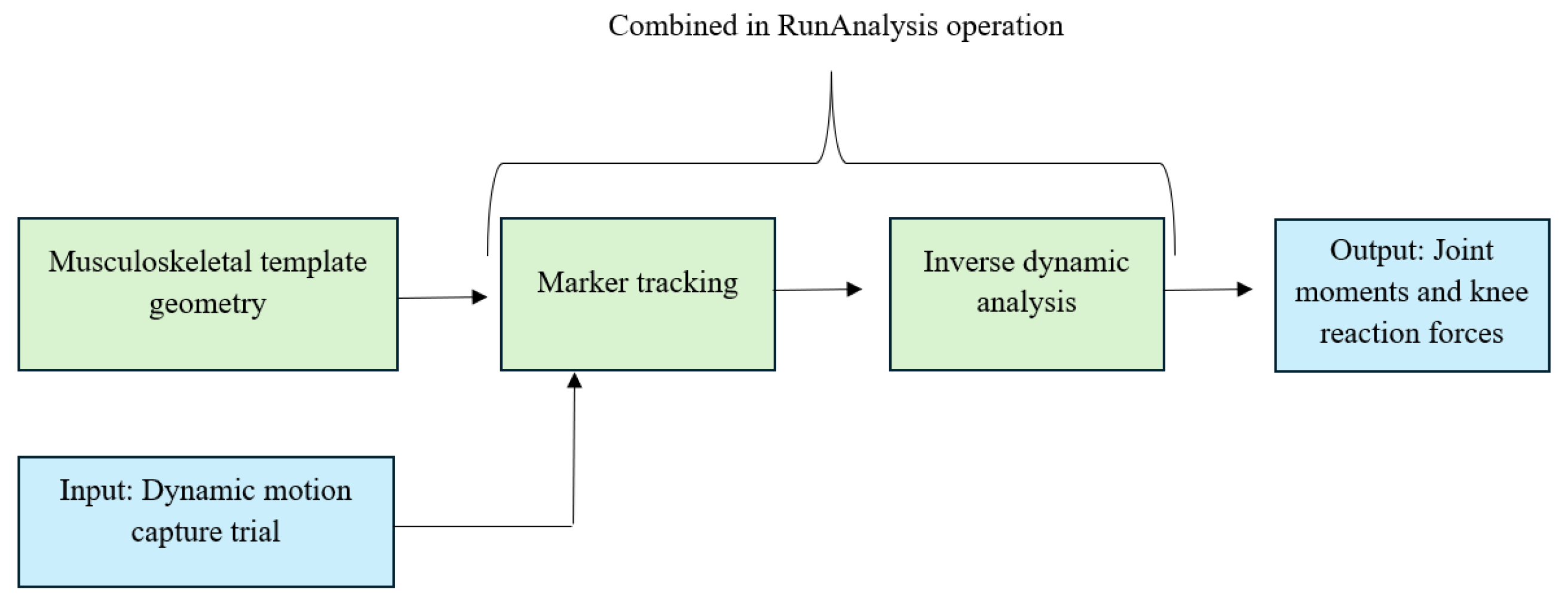
2.3. Musculoskeletal Model

The musculoskeletal simulations were performed using the AnyBody Modeling System (AMS, version 8.0, AnyBody Technology, Aalborg, Denmark). The base model employed was the BVH_Xsens model, available within the AnyBody Managed Model Repository (AMMR, version 3.0.4), which includes a detailed full-body representation suitable for gait analysis [15]. This AMMR model is built upon anatomical data derived from cadaver studies, providing anatomically accurate segmental representations for biomechanical simulations. This model incorporates lower and upper extremity segments, major muscle groups, and joint kinematics driven by motion capture data.

Several subject-specific adaptations were performed:

• LabSpecificData: this part ensures that ground contact is correctly detected (indicated by red spheres). In this case, the ground contact threshold was adjusted to 0.045 for both legs, as this parameter significantly affects knee joint forces;
• SubjectSpecificData: the subject’s weight and height are set according to their specific characteristics.
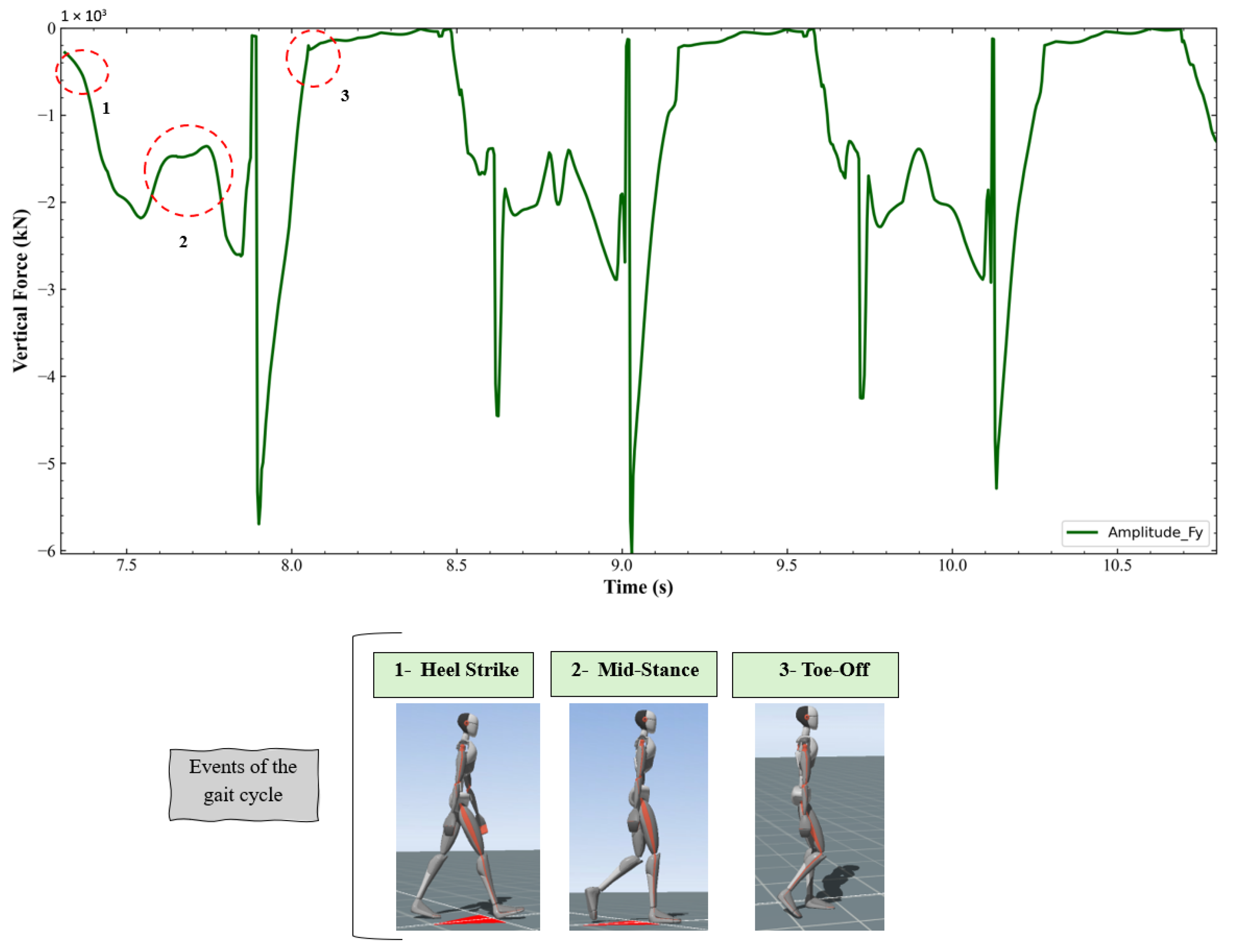
• TrialSpecificData: the start and end frames of the analyzed trial were set to 10 and 300, respectively. Only the frames corresponding to forward walking, i.e., when the subject moved in the positive direction of the gait cycle, were considered for analysis. This ensured that the musculoskeletal modeling focused exclusively on the phases of consistent and natural forward locomotion, minimizing variability due to turns or changes in walking direction.
• AnyMocap Model: used to drive the musculoskeletal simulation using the processed motion capture data.

These adjustments ensured that the model accurately represented the participant’s movement and loading conditions during gait analysis.

After configuring the customized MS model, inverse dynamics were applied to estimate the internal joint forces and moments based on the captured kinematic data. Inverse dynamics involves computing the net joint forces and moments required to produce a measured motion, considering the body’s mass distribution and inertial properties. Using the joint angles derived from motion capture, the AnyBody software employed the Newton–Euler equations of motion to calculate joint reaction forces and moments throughout the gait cycle [16], as illustrated by Figure 3.

In this initial phase, only the bone structures of the femur and tibia were considered, with ligament integration planned for a later stage. To enable integration between the AnyBody MS model and the FE knee model developed by Santos et al. [17], the femur and tibia geometries were isolated and exported as stereolithography (STL) files. Within the LabSpecificData section, a new file was created to include the design of each separated structure. The geometries were drawn and visualized using the AnyDrawSurf class, applying a scaling factor of 0.001 to convert units from millimeters to meters. Alignment of the STL models to the human anatomy in AnyBody was achieved via a rigid-body transformation using the AnyFunTransform3DLin2 object. The transformation mode was set to VTK_LANDMARK_RIGIDBODY, ensuring that only rotation and translation were applied, without any scaling [18]. This alignment was based on anatomical landmarks, providing an initial spatial registration between the customized knee geometries and the musculoskeletal model:

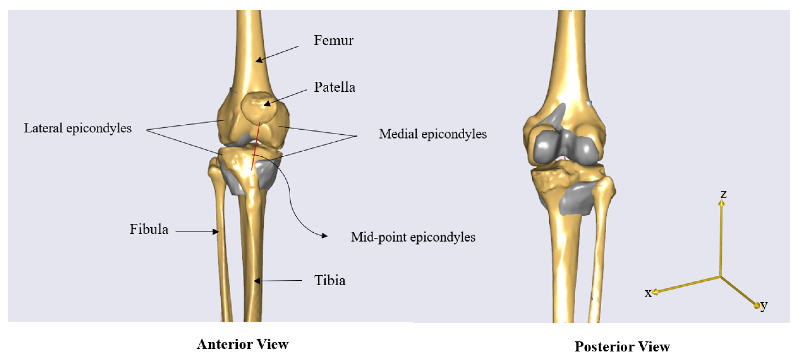
• Points 0: Source landmarks extracted from the STL files, including the medial and lateral femoral epicondyles, their midpoint, the KneeJointAnatomicalFrame for the femur, and the TibialTuberosity for the tibia.
• Points 1: Target landmarks defined within the AnyBody model’s anatomical hierarchy.

This method generally ensures accurate spatial alignment between the customized knee geometries and the existing musculoskeletal model. However, after reloading the model, the bones appeared partially merged in the Model View, as shown in Figure 4. This suggests that a more refined scaling approach may be required, potentially using transformation functions such as AnyFunTransform3DRBF or AnyFunTransform3DSTL to improve the alignment and morphology fitting.

Within the LabSpecificData.any file, a specific code is included to define the extraction process of the forces acting on the tibia. Initially, the forces and moments for the right tibia were measured, including those generated by muscles (such as the psoas major) and joint reactions in the knee. Additionally, the code accounts for the effects of gravity and inertia. The extracted forces and moments are subsequently transformed into the anatomical reference frame of the tibia, ensuring that their orientation is correct for use in later simulations, such as those conducted in Abaqus.

Finally, net knee forces (F) and moments (M) acting on the right tibia in three directions (x, y, z) were extracted based on the inverse dynamics study. These forces are saved in a CSV file for subsequent analysis. It is important to note that the forces and moments are only extracted for the right knee, as the 3D model used in the simulations corresponds to the right knee joint specifically.

2.4. Abaqus

The FE model of the knee used in this study was initially adapted from the Open Knee Project [19], an important open-source initiative that promotes scientific advancement. The model’s geometry was reconstructed from MRI scans of a 70-year-old female cadaveric donor, with a body mass of 77.1 kg and a height of 1.68 m. The model was later adapted by Santos et al. [17], and includes the bones (femur and tibia), the articular cartilages (both femoral and tibial, lateral, and medial), the major ligaments (anterior cruciate, posterior cruciate, medial collateral, and lateral collateral), and the menisci (lateral and medial). In this study, the adapted version by Santos et al. [17] was directly employed to ensure anatomical and biomechanical realism in the FE simulations, as illustrated in Figure 5.

The motion capture data used to inform the boundary conditions were collected from a female subject with similar body proportions to those of the cadaveric donor. Although age-related differences in tissue properties may influence joint behavior, this approximation was deemed acceptable for preliminary analysis. Future work will involve reconstructing the FE model using MRI data from the same subject used in the motion capture trials, allowing for a more individualized and physiologically consistent simulation.

While this model provides a robust basis for simulating joint biomechanics, it is important to acknowledge certain limitations and potential areas for future enhancement. In particular, the inclusion of the patella and its associated soft tissues such as the quadriceps tendon, the patellar ligament, the medial and lateral patellar retinaculum, and the medial patellofemoral ligament (MPFL) could significantly improve the anatomical fidelity of the model. These structures play a key role in patellofemoral joint stability and load distribution, and their integration would allow for more comprehensive simulations, particularly in scenarios involving knee extension, anterior knee pain, or patellar tracking disorders.

The material properties assigned to each anatomical structure used in the FE model are summarized in

Table 2. Material properties of the anatomical structures used in the FE model, adapted from [20].

Structure	Material Type	Constitutive Parameters
Femur/Tibia	Elastic	$E=17,400$ MPa, $\nu =0.30$
Articular Cartilage	Elastic	$E=80$ MPa, $\nu =0.475$
Menisci	Elastic	$E=120$ MPa, $\nu =0.45$
ACL Connective Tissue	Hyperelastic (Neo–Hookean)	$C_{10}=1.0$ MPa, $D_1=1\times {10}^{-5}$ ${\mathrm{MPa}}^{-1}$
Anterior Cruciate Ligament	Anisotropic Hyperelastic (HGO)	$K_1=52.52$ MPa, $K_2=5.86$, $K=0.0$ ${\mathrm{MPa}}^{-1}$
Posterior Cruciate Ligament	Anisotropic Hyperelastic (HGO)	$K_1=46.42$ MPa, $K_2=2.73$, $K=0.0$ ${\mathrm{MPa}}^{-1}$
Lateral Collateral Ligament	Anisotropic Hyperelastic (HGO)	$K_1=41.21$ MPa, $K_2=5.26$, $K=0.0$ ${\mathrm{MPa}}^{-1}$
Medial Collateral Ligament	Anisotropic Hyperelastic (HGO)	$K_1=41.01$ MPa, $K_2=5.07$, $K=0.0$ ${\mathrm{MPa}}^{-1}$

. For linear elastic materials, the parameters include Young’s modulus (E), which defines the stiffness, and Poisson’s ratio ($\nu$, dimensionless), which describes the material’s lateral deformation under uniaxial stress. For hyperelastic materials, parameters $C_{10}$ and $D_1$ correspond to the Neo-Hookean model. Here, $C_{10}$ characterizes the shear response, while $D_1$ governs material compressibility. For anisotropic hyperelastic behavior, the Holzapfel–Gasser–Ogden (HGO) model is used, with parameters $K_1$, $K_2$, and K. In this context, $K_1$ and $K_2$ define the fiber-related stress response, while K controls bulk incompressibility.

The analysis was carried out through a static general step, suitable for evaluating equilibrium states under external loading. A maximum number of 4000 increments was specified to ensure convergence, particularly in early simulations with potentially complex contact or boundary conditions. The initial increment size was set to 0.05, with a minimum increment size of $1\times {10}^{-10}$ and a maximum of 1, allowing Abaqus to automatically adjust the increment size to maintain numerical stability and convergence throughout the simulation.

To ensure proper connectivity between independent FE meshes, surface-to-surface tie constraints were applied. This type of tie was chosen because it allows for more accurate force transmission over contact areas, especially when the meshes do not have a node-to-node match, a common scenario in anatomical models with complex geometry. The applied tie constraints were organized as follows:

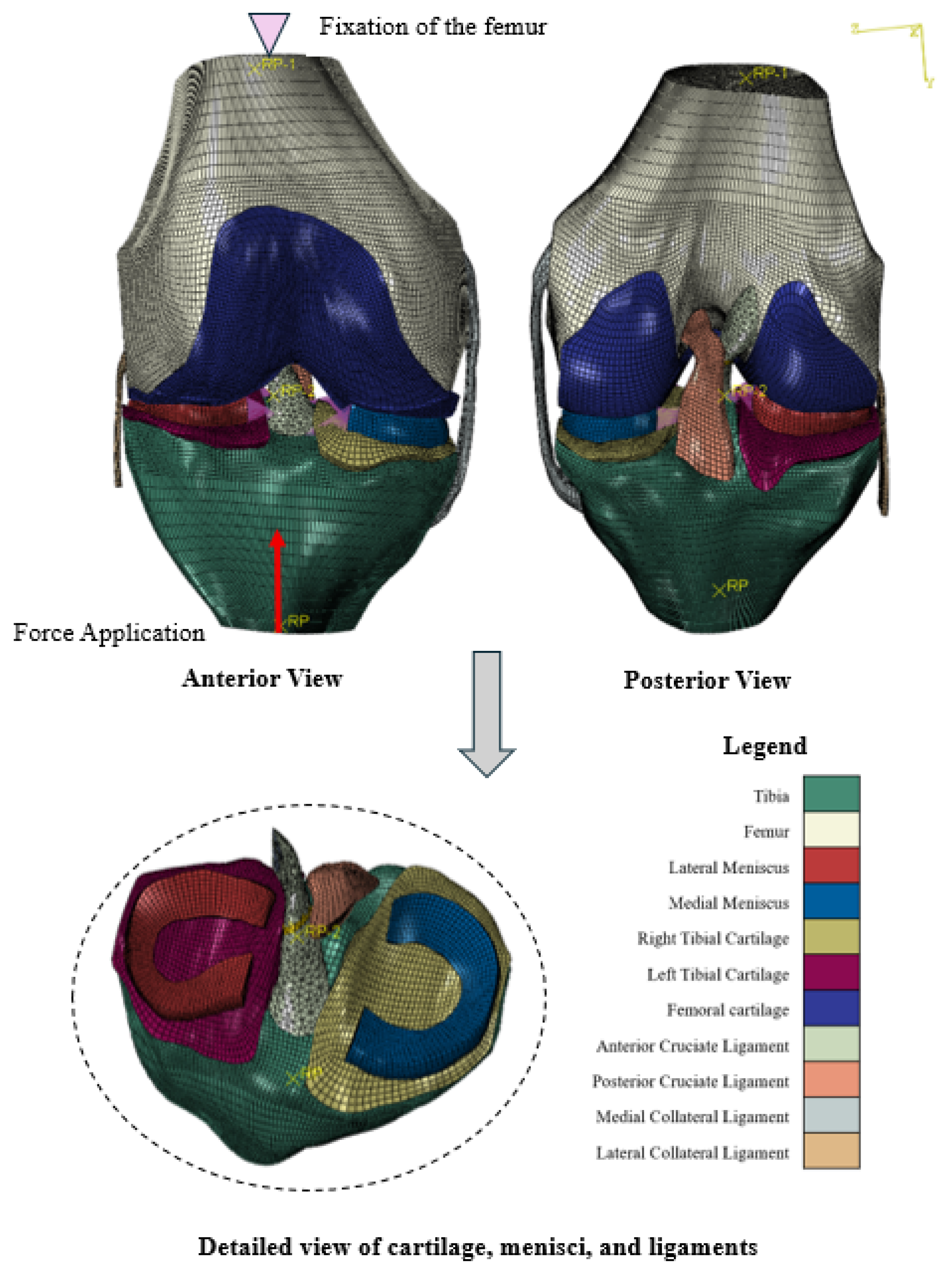
• Ligament-to-bone connections:

  –

  Medial collateral ligament (MCL), ACL, and posterior cruciate ligament (PCL) to femur and tibia;

  –

  Lateral collateral ligament (LCL) to femur (note: anatomically, the LCL inserts on the fibula, which is not yet included in the current model but is intended to be added in future developments);

• Cartilage-to-bone connections:

  –

  Left and right tibial cartilage to tibia;

  –

  Femoral cartilage to femur;

The femur and tibia were defined as rigid bodies, as their deformation is negligible compared to that of soft tissues. This assumption reduces computational cost while preserving the accuracy of soft tissue interaction. These constraints ensured that all connected structures moved together during the simulation, accurately representing physiological bonding between tissues.

In addition to the tie constraints, a surface-to-surface contact interaction was defined. This type of contact models the physical interaction between two deformable surfaces, allowing them to come into contact, transmit forces, and potentially separate unlike tie constraints, which assume perfectly bonded behavior. A “hard” contact formulation was used, meaning that no penetration is allowed between the surfaces in the normal direction, while tangential behavior (such as friction) can be adjusted as needed. This contact definition was not limited to the interfaces between the menisci and the femoral and tibial cartilage; it was also applied to the interactions between the following structures:

• Between the surfaces of the left tibial cartilage and the femoral cartilage;
• Between the surfaces of the right tibial cartilage and the femoral cartilage;
• Between the surfaces of the ACL and the PCL.

For the preliminary phase of the study, simplified boundary conditions were adopted to evaluate the general behavior of the system before implementing more physiologically accurate constraints. Before proceeding with the load definition in Abaqus, an amplitude–time curve was generated from experimental gait data. Time values (in seconds) were assigned to the X-axis, and vertical force values at the knee joint (Fy component) to the Y-axis, forming a tabular dataset. The resulting plot is shown in Figure 6.

As observed in Figure 6, the raw data include transient peaks exceeding 6 kN. These were attributed to abrupt motion transitions or noise artifacts and were subsequently removed through filtering. Typical force values range from 2 to 3 kN, which reflect the knee loading pattern of an overweight individual (based on BMI classification) during normal walking. Even in the unfiltered data, key features of the stance phase in the gait cycle can be observed. These include an initial peak corresponding to heel strike, when the heel makes contact with the ground and vertical force rises sharply; a mid-stance valley, where body weight is supported over the leg and force temporarily decreases; and a second peak related to toe-off, when the foot pushes off the ground to propel the body forward [21]. The filtered and time-aligned force profile was then used as an amplitude input for defining the loading conditions in Abaqus.

Regarding the boundary conditions, a velocity constraint was applied to simulate rotational movement, with the initial velocity set to 0 m/s. This ensured that the femur remained stationary at the start of the simulation, preventing unwanted movements or numerical instabilities. By doing so, the system was initialized from a fixed and stable position, allowing the forces and reactions at the joints to be properly assessed during the simulation.

For the tibia, a concentrated force (CF) was applied with a CF2 factor of −1 N, representing the force the tibia applies on the femur. This force was modeled based on physiological and anatomical conditions, taking into account the natural interaction between these two structures during movement. The amplitude curve, which was previously explained, was used to describe how the force varies over time, adjusting the load realistically throughout the movement cycle. The values of this force were then multiplied by the CF2 factor, adjusting the magnitude of the force applied. The CF2 factor acts as a scaling factor, adjusting the intensity of the force according to the specific model parameters and experimental conditions. This ensures that the force applied to the tibia is represented accurately and realistically during the simulation. Figure 7 illustrates the applied boundary conditions:

To summarize, the boundary conditions applied in the FE model were derived from the outputs of the MS simulation performed in AnyBody. Specifically, the net knee forces were extracted as a force–time curve and used as a time-dependent external load in Abaqus. Due to geometric misalignments between the STL mesh in Abaqus and the anatomical representation in AnyBody, it was not feasible to apply forces at anatomically precise insertion points or fully replicate detailed joint mechanics. Therefore, a simplified approach was adopted, enabling a practical approximation of joint loading during gait while ensuring numerical stability and compensating for the geometric discrepancies between the two modeling environments.

Table 3. Number of elements and nodes used in the FE mesh for each anatomical structure, adapted from [17].

Structure	Elements	Nodes
Femur	13,860	13862
Tibia	11,360	11,362
Articular Cartilage	25,721	35,712
Menisci	9100	11,616
ACL Connective Tissue	3875	1288
ACL	3000	3796
PCL	5248	5922
LCL	6656	7425
MCL	5120	5781

presents the number of elements and nodes for each of the structures included in the model. For both the femur and tibia, the element type used is S4, which is a 4-node shell element suitable for modeling thin-walled structures. These elements have a quadrilateral shape, allowing accurate representation of curved surfaces with reduced computational cost.

For the remaining structures listed in Table 3, the element type used is C3D8H, an 8-node linear hexahedral element with a hybrid formulation, commonly employed for modeling nearly incompressible materials such as biological soft tissues. These elements have a hexahedral shape. An exception is made for the connective tissue of the ACL, for which C3D4H elements were used. These are 4-node linear tetrahedral elements, also with a hybrid formulation, and are better suited for capturing complex geometries where structured hexahedral meshing is not feasible. A mesh verification was performed to ensure the quality and reliability of the FE discretization. This process included checking for element distortion, aspect ratio, and the convergence of results with respect to mesh refinement. The final mesh comprised 84.810 elements, with no analysis errors detected (0%), indicating proper mesh generation and element integrity. Although 8.578 analysis warnings were reported (approximately 10%), a thorough review confirmed that they did not compromise the overall accuracy or stability of the simulation. The selected mesh thus provided a good balance between numerical accuracy and computational efficiency.

Then, a job was created and executed using the Abaqus/Standard 2024 solver, which is well-suited for the non-linear, quasi-static analysis of elastic and anisotropic hyperelastic materials used in the model.

In the results visualization section, the distribution of the maximum principal stresses (S, Max. Principal) in the tibial component of the knee under physiological loading conditions was evaluated. The stress output was displayed with nodal averaging set to 75%, meaning that only a subset of the surrounding elements were considered when calculating the nodal values. This averaging technique helps smooth out artificial stress discontinuities at element boundaries, improving the interpretability of the results without overly distorting localized stress concentrations. For analysis along a specific trajectory, a path was defined based on nodal positions, beginning at the femoral attachment location (start frame) and ending at the tibial insertion (end frame). The horizontal axis shows the true distance along the path (in mm), while the vertical axis represents the stress (in MPa), and specifically, the maximum principal stress extracted from the simulation results. In addition, a displacement analysis was carried out along two different paths. The first was plotted from the distal end of the tibia to the anatomical insertion location of the ACL. The second path, also in the ACL region, followed the anatomical direction of the ligament, starting at the femoral attachment and ending at the tibial insertion. These trajectories are a detailed assessment of the deformation patterns along the ligament and bone structures involved.

3. Results and Discussion

The participant demonstrated excellent knee function, with a KOOS score of 98 and an IKDC score of 98.9, indicating high levels of recovery and minimal functional impairment. These scores provide a solid clinical foundation for the subsequent biomechanical simulation analysis using Abaqus.

The results are illustrated in Figure 8, which shows the distribution of maximum principal stresses from anterior and posterior views of the model.

The stress values range from approximately −28.67 MPa (dark blue) to +44.95 MPa (red). In both views, a predominance of green tonalities can be observed, especially across the medial and lateral tibial plateaus, indicating that these regions are mainly subjected to mild compressive stresses, consistent with axial load transmission through the joint. Areas located near the intercondylar region show a slightly more intense green color, suggesting areas of moderate tensile stress, probably related to contact pressure peaks or ligament insertions.

In the region of the tibial plateau, the simulation revealed stress values ranging from approximately 2 to 8 MPa, which align reasonably well with the values reported for normal gait, typically ranging between 2 and 6 MPa [8]. This may indicate that, after surgery, the patient has recovered a biomechanically functional joint, capable of distributing loads in a manner consistent with the physiological behavior of the joint during gait. However, a more in-depth analysis of muscle forces would be necessary to reflect realistic joint mechanics. In addition, extending the analysis to a larger sample of individuals would be essential to account for inter-individual variability and to draw more generalizable conclusions about post-surgical knee function.

Following the simulation, the graph shown in Figure 9 was plotted to represent the variation of stress along the true distance along the path of the ACL.

At the beginning of the path (near 0 mm), a pronounced stress peak is observed, reaching approximately 1.45 MPa, indicating a region of high tensile loading close to the femoral insertion. This aligns with findings by Shi et al., who reported that the femoral attachment site of the ACL experiences higher stress compared to the tibial attachment, with stress levels notably elevated during the initial phases of landing [22]. Immediately after this peak, the stress decreases abruptly to around 0.4 MPa, and then gradually decreases along the remainder of the ligament. From about 5 mm onward, the stress values remain relatively low, fluctuating slightly around 0.0 to 0.2 MPa. Notably, there is also an initial dip to a negative stress value close to –3.0 MPa, which may correspond to localized compression or a transition zone near the fixation point.

This non-uniform distribution of stress suggests that the proximal region of the ACL (closer to the femur) supports a substantially greater portion of the load under the current boundary conditions where the femur is fixed and a load is applied to the tibia while the distal region (towards the tibia) is subject to lower stress levels or slight unloading. These findings reflect the typical mechanical behavior of the ACL, influenced by its curved anatomical path and the direction of applied force.

To complement the stress analysis, a displacement study was performed to evaluate the mechanical response of the knee joint under the applied loading conditions. Figure 10 illustrates the magnitude of the total displacement (U) across the joint structure, incorporating all directional components.

The color scale indicates displacement values in millimeters (mm), ranging from 0 mm (dark blue) in fully constrained areas to a maximum of approximately 1.068 mm (red) in the areas of greatest movement. The highest displacement values are observed in the distal part of the tibia, which was the region subjected to loading in the simulation, while the femur remains mostly stationary due to the boundary conditions (fully fixed). Intermediate displacement values, represented by green to yellow colors, are visible in the lower and middle tibial regions and surrounding soft tissues. This gradient reflects the mechanical transition from the fixed femoral region to the loaded tibial extremity, with a smooth distribution of deformation along the joint. This displacement pattern confirms the mechanical effect of the applied loading scenario, resulting in tibial motion predominantly in the downward and anterior directions relative to the femur, consistent with the expected biomechanical behavior of the knee joint.

To provide a more localized understanding of the deformation behavior under load, Figure 11 presents the displacement along the tibial structure. This analysis offers insight into how displacement varies through the tibial structure under the given boundary conditions.

The graph displays a gradual and continuous decline in displacement as the path progresses proximally. The maximum displacement, occurring at the distal point where the load is applied, is approximately 0.99 mm, while the displacement near the ACL insertion is reduced to around 0.83 mm. These displacement values are consistent with ranges reported in the literature for FE models of the knee, which typically exhibit displacements between 0.5 mm and 2 mm depending on the applied load magnitude and the material properties of the involved tissues. In particular, Wu et al. [23] reported a distal tibial displacement of 1.10 mm under a comparable loading condition. Although a slight variation exists, the difference from the current simulation is only 0.11 mm, which supports the validity of the present model and suggests a strong agreement with previous FE analyses.

To gain further understanding of the localized deformation of the ACL region, Figure 12 shows the displacement magnitude plotted as a function of the true distance along the ligament’s anatomical direction.

The graph reveals a non-linear displacement distribution along the ligament trajectory. Displacement increases steeply in the initial segment, reaching approximately 0.55 mm around 7–8 mm along the path. Following this peak, a slight decrease is observed, suggesting localized stiffening or constraint in the mid-portion of the ligament path, with a minimum around 0.45 mm. Beyond this point, displacement continues at a steady increase, reaching approximately 0.80 mm near the tibial insertion. This non-monotonic pattern reflects the complex mechanical response of the ACL region under compressive loading. The variation in displacement may be attributed to local geometric transitions, contact conditions, or the alignment of the ligament relative to surrounding bone. The increase in displacement towards both ends of the path is consistent with boundary conditions where bone segments are differentially loaded or constrained. According to the article by Mao et al. [24] with the distal tibia fixed and the femur free, a load between 500 and 800 N was applied, resulting in displacements of approximately 2.5 mm in the femoral tunnel, 1 mm in the intra-knee region, and 0.50 mm in the tibial tunnel. Although the displacement values reported here are lower, this difference may be attributed to specific boundary conditions employed in the study, such as the fixation of the femur and the application of load on the tibia. However, both studies come to the same conclusion: displacement is smallest near the tibial insertion, increases through the medial portion, and reaches its greatest value at the femoral side.

Despite some limitations, this study introduces a novel approach by combining subject-specific gait data from wearable sensors with FE simulations of the knee after ACL reconstruction. This integration allows more realistic and personalized analysis of ligament mechanics during movement, improving on generic models. Although based on a single case and simplified conditions, the pipeline demonstrates potential for enhancing surgical planning and rehabilitation by capturing individual biomechanical behavior.

4. Conclusions

The biomechanical analysis suggests that the subject has recovered well post-surgery, with minimal functional limitations and restored knee performance. The FE simulation displayed a characteristic stress distribution in the tibial component under physiological loading, marked by compressive stresses over the medial and lateral tibial plateaus indicative of normal, axial load transfer through the joint. Displacement results corroborated this response, with maximal deformation observed in the loaded distal tibia, while the femur remained largely stationary due to fixed boundary conditions. Along the anatomical path of the ACL, displacement followed a non-linear curve, highlighting the ligament’s complex mechanical behavior under load. Overall, the joint exhibited biomechanical patterns consistent with normal gait, supporting the conclusion of functional recovery. While the current study provides valuable insights into tissue stress following ACL reconstruction, it is important to acknowledge that the conclusions are based primarily on stress analysis alone. Comprehensive biomechanical evaluation, including joint kinematics, kinetics, such as knee abduction and rotational moments, and subject-specific muscle forces, was not incorporated in this work. These factors are known to significantly influence joint loading and function and should be considered for a more complete understanding of post-operative knee biomechanics. Future research will focus on integrating these parameters to enhance the physiological accuracy of the models and enable more robust, clinically meaningful conclusions regarding rehabilitation outcomes.

Several important improvements can be made to further increase the model’s accuracy and clinical relevance. The AnyBody musculoskeletal model does not currently include ligament structures, such as the ACL, which have a fundamental role in maintaining knee stability and the orientation of the joint’s mechanics. Although the model incorporates essential aspects of knee function, incorporating these ligaments in future iterations would probably improve the representation of joint constraints and load distribution, leading to more accurate simulations. Similarly, the FE model could benefit from the inclusion of additional anatomical components, such as the patella, associated ligaments, and fibula. These elements are known to contribute significantly to load distribution and joint stability, and their integration would increase the physiological fidelity of the model. An additional relevant consideration is the use of MRI data from a different subject in the current FE model. Although this approach has been adequate for developing and testing the modeling framework, it may limit anatomical specificity and reduce the physiological relevance of the simulations. Using a FE model that corresponds to the same subject from which gait data was collected would improve anatomical consistency between datasets, leading to more accurate representations of joint geometry, tissue loading, and overall knee function. This alignment would support more personalized and clinically significant biomechanical knowledge. Another key improvement would be the application of morphing techniques using MRI data to generate more precise, patient-specific anatomical models. This would ensure better alignment between gait analysis and the FE model, enabling a more individualized simulation. In future work, marker-based motion capture will be incorporated and compared with IMU-based results in order to assess the accuracy and clinical applicability of both approaches.

Finally, the integration of clinical data with biomechanical modeling tools could be streamlined through a semi-automatic pipeline. By using Python 3.13.5 scripts in an integrated development environment like Spyder, data from motion capture systems could be processed and converted into formats compatible with MS modeling software, which would then run simulations to generate joint forces and muscle activations. These results could be directly transferred to the FE model for further analysis, significantly reducing manual intervention and improving consistency across simulations. This approach has the potential to automate the workflow, enabling more efficient and scalable analysis across multiple subjects or trials in future applications. The development of this semi-automated process could offer significant benefits for clinicians and researchers by facilitating the rapid generation of personalized FE models using clinical data such as MRI and real-time motion data. This would streamline simulations, enhance treatment plan accuracy, and support more individualized rehabilitation strategies.

References

1. Zhang, L.; Liu, G.; Han, B.; Wang, Z.; Yan, Y.; Ma, J.; Wei, P. Knee Joint Biomechanics in Physiological Conditions and How Pathologies Can Affect It: A Systematic Review. Appl. Bionics Biomech. 2020, 2020, 7451683. [Google Scholar] [CrossRef] [PubMed]
2. Halloran, J.P.; Ackermann, M.; Erdemir, A.; van den Bogert, A.J. Concurrent Musculoskeletal Dynamics and Finite Element Analysis Predicts Altered Gait Patterns to Reduce Foot Tissue Loading. J. Biomech. 2010, 43, 2810–2815. [Google Scholar] [CrossRef] [PubMed]
3. Peitola, J.P.J.; Esrafilian, A.; Eskelinen, A.S.A.; Andersen, M.S.; Korhonen, R.K. Sensitivity of knee cartilage biomechanics in finite element analysis to selected Musculoskeletal models. Comput. Methods Biomech. Biomed. Eng. 2024, 1–12. [Google Scholar] [CrossRef] [PubMed]
4. Shu, L.; Yamamoto, K.; Yoshizaki, R.; Yao, J.; Sato, T.; Sugita, N. Multiscale finite element musculoskeletal model for intact knee dynamics. Comput. Biol. Med. 2022, 141, 105023. [Google Scholar] [CrossRef] [PubMed]
5. Karimi Dastgerdi, A.; Esrafilian, A.; Carty, C.P.; Lloyd, D.G.; Saxby, D.J. Validation and evaluation of subject-specific finite element models of the pediatric knee. Sci. Rep. 2023, 13, 18328. [Google Scholar] [CrossRef] [PubMed]
6. Tan, T.; Gatti, A.A.; Fan, B.; Shea, K.G.; Sherman, S.L.; Uhlrich, S.D.; Hicks, J.L.; Delp, S.L.; Shull, P.B.; Chaudhari, A.S. A scoping review of portable sensing for out-of-lab anterior cruciate ligament injury prevention and rehabilitation. NPJ Digit. Med. 2023, 6, 46. [Google Scholar] [CrossRef] [PubMed]
7. Cox, K.; Hamrock, D.; Lawrence, S.; Lynch, S.; Romness, J.; Saksvig, J.; Warner, A.; Gutierrez, R.; Hart, J.; Boukhechba, M. How wearable sensing can be used to monitor patient recovery following ACL reconstruction. In Proceedings of the 2022 Systems and Information Engineering Design Symposium (SIEDS), Charlottesville, VA, USA, 28–29 April 2022; pp. 234–239. [Google Scholar] [CrossRef]
8. Halonen, K.S.; Dzialo, C.M.; Mannisi, M.; Venäläinen, M.S.; de Zee, M.; Andersen, M.S. Workflow assessing the effect of gait alterations on stresses in the medial tibial cartilage—Combined musculoskeletal modelling and finite element analysis. Sci. Rep. 2017, 7, 17396. [Google Scholar] [CrossRef] [PubMed]
9. Andres, A.; Roland, M.; Wickert, K.; Ganse, B.; Pohlemann, T.; Orth, M.; Diebels, S. Individual postoperative and preoperative workflow for patients with fractures of the lower extremities. Clin. Biomech. 2025, in press. [Google Scholar] [CrossRef] [PubMed]
10. Abdullah, M.; Hulleck, A.A.; Katmah, R.; Trebes, N.; Damm, P.; Duda, G.N.; List, R.; Trepczynski, A. Multibody dynamics-based musculoskeletal modeling for gait analysis: A systematic review. J. Neuroeng. Rehabil. 2024, 21, 178. [Google Scholar] [CrossRef] [PubMed]
11. Ebenbichler, M.; Heinrich, D.; Mohr, M.; Ueno, R.; Eberle, R. Coupling a finite element knee model with musculoskeletal multibody simulations. A case study of ACL force during a change-of-direction movement before and after injury prevention training. Curr. Issues Sport Sci. (CISS) 2024, 9, 004. [Google Scholar] [CrossRef]
12. Movella. Five Steps to Quickly Set Up Your Xsens In-home Mocap Studio. 2020. Available online: https://www.movella.com/resources/blog/five-steps-to-set-up-your-xsens-in-home-studio (accessed on 28 April 2025).
13. AnyBody Technology. The AnyBody Modeling System. 2024. Available online: https://www.anybodytech.com/ (accessed on 28 April 2025).
14. Dassault Systèmes. Abaqus Unified FEA. 2024. Available online: https://www.3ds.com/products-services/simulia/products/abaqus/ (accessed on 28 April 2025).
15. Lund, M.E.; Chander, D.S.; Galibarov, P.; Tørholm, S.; Engelund, B.K.; Shayestehpour, H.; Damsgaard, M. The AnyBody ManagedModel Repository (AMMR). 2025. Version 3.1.0. Available online: https://www.anybodytech.com/software/ammr/ (accessed on 28 April 2025).
16. Andersen, M.S. 4—Introduction to musculoskeletal modelling. In Computational Modelling of Biomechanics and Biotribology in the Musculoskeletal System, 2nd ed.; Jin, Z., Li, J., Chen, Z., Eds.; Woodhead Publishing Series in Biomaterials; Woodhead Publishing: Sawston, UK, 2021; pp. 41–80. [Google Scholar] [CrossRef]
17. Santos, C.F.; Bastos, R.; Andrade, R.; Pereira, R.; Parente, M.P.L.; Jorge, R.N.; Espregueira-Mendes, J. Revisiting the Role of Knee External Rotation in Non-Contact ACL Mechanism of Injury. Appl. Sci. 2023, 13, 3802. [Google Scholar] [CrossRef]
18. AnyBody Technology. Scaling and Personalizing Your Model—Lesson 1. 2024. Available online: https://anyscript.org/tutorials/Scaling/lesson1.html (accessed on 29 April 2025).
19. Erdemir, A. Open Knee: Open Source Modeling and Simulation in Knee Biomechanics. J. Knee Surg. 2016, 29, 107–116. [Google Scholar] [CrossRef] [PubMed]
20. Kubicek, M.; Florian, Z. Stress Strain Analysis of Knee Joint. Eng. Mech. 2009, 16, 315–322. [Google Scholar]
21. Completo, A.; Fonseca, F. Fundamentos de Biomecânica Músculo-Esquelética e Ortopédica, 2nd ed.; Medicabook: Lisbon, Portugal, 2019; p. 444. [Google Scholar]
22. Shi, H.; Yu, Y.; Huang, H.; Li, H.; Ren, S.; Ao, Y. Biomechanical Determinants of Anterior Cruciate Ligament Stress in Individuals Post—ACL Reconstruction During Side-Cutting Movements. Bioengineering 2025, 12, 222. [Google Scholar] [CrossRef] [PubMed]
23. Wu, C.C.; Ye, L.M.; Li, X.F.; Shi, L.J. Sequential damage assessment of the posterolateral complex of the knee joint: A finite element study. J. Orthop. Surg. Res. 2022, 17, 185. [Google Scholar] [CrossRef] [PubMed]
24. Mao, Z.M.; Wang, Z.W.; Xu, C.; Liu, C.H.; Zhang, Z.Y.; Ren, X.L.; Xue, A.Q.; Li, Z.N.; Zhao, F.; Yao, Q.; et al. Intra-Articular Biomechanical Changes of the Meniscus and Ligaments During Stance Phase of Gait Circle after Different Anterior Cruciate Ligament Reconstruction Surgical Procedures: A Finite Element Analysis. Orthop. Surg. 2022, 14, 3367–3377. [Google Scholar] [CrossRef] [PubMed]
Figure 1. Illustration of the biomechanical simulation workflow, integrating motion capture data with MS and FE modeling. The workflow adapts the FE model using patient-specific imaging, achieved through semi-automatic segmentation and morphing techniques for anatomical personalization.
Biomechanics 05 00057 g001
Figure 2. Calibration postures: (A) N-pose (standard), with arms aligned vertically alongside the body and (B) T-pose (alternative), with arms abducted horizontally at shoulder height.
Biomechanics 05 00057 g002
Figure 3. Schematic representation of the inverse dynamics process, in which joint forces and moments are estimated based on the motion data and segmental inertial properties of the system.
Biomechanics 05 00057 g003
Figure 4. Main anatomical reference points—epicondyles, KneeJointAnatomicalFrame, and tibial tuberosity—used to align and transform the STL geometries of the femur and tibia. The image also illustrates the partial fusion of these bones observed in the AnyBody Model View after alignment.
Biomechanics 05 00057 g004
Figure 5. Simplified 3D model of the knee joint, where the femur is shown in beige and the tibia in dark green.
Biomechanics 05 00057 g005
Figure 6. Representation of time as a function of the vertical raw force of the knee joint and identification of the principal gait events: heel strike (1)—the moment when the heel contacts the ground; mid-stance (2)—where body weight is directly over the supporting leg; and toe-off (3)—the toes leave the ground as the leg moves forward.
Biomechanics 05 00057 g006
Figure 7. Illustration of the boundary conditions, with the femur fixed at the top and a concentrated force (CF) applied to the bottom of the tibia. The figure also shows the reference structure adopted for this model.
Biomechanics 05 00057 g007
Figure 8. Maximum principal stress distribution on the model, shown from anterior (left) and posterior (right) views.
Biomechanics 05 00057 g008
Figure 9. Stress distribution along the ACL as a function of the true distance along the path from the femoral to the tibial insertion.
Biomechanics 05 00057 g009
Figure 10. Total displacement magnitude (U, Magnitude) of the knee joint under loading conditions, displayed in both anterior (left) and posterior (right) views.
Biomechanics 05 00057 g010
Figure 11. Displacement magnitude plotted along a path from the distal tibia to the ACL insertion region.
Biomechanics 05 00057 g011
Figure 12. Displacement magnitude along the anatomical trajectory of the ACL, from its tibial insertion to femoral attachment.
Biomechanics 05 00057 g012