Virgin Passive Colon Biomechanics and a Literature Review of Active Contraction Constitutive Models

Abstract

The objective of this paper is to present our findings on the biomechanical aspects of the virgin passive anisotropic hyperelasticity of the porcine colon based on equibiaxial tensile experiments. Firstly, the characterization of the intestine tissues is discussed for a nearly incompressible hyperelastic fiber-reinforced Holzapfel–Gasser–Ogden constitutive model in virgin passive loading conditions. The stability of the evaluated material parameters is checked for the polyconvexity of the adopted strain energy function using positive eigenvalue constraints of the Hessian matrix with MATLAB. The constitutive material description of the intestine with two collagen fibers in the submucosal and muscular layer each has been implemented in the FORTRAN platform of the commercial finite element software LS-DYNA, and two equibiaxial tensile simulations are presented to validate the results with the optical strain images obtained from the experiments. Furthermore, this paper also reviews the existing models of the active smooth muscle cells, but these models have not been computationally studied here. The review part shows that the constitutive models originally developed for the active contraction of skeletal muscle based on Hill’s three-element model, Murphy’s four-state cross-bridge chemical kinetic model and Huxley’s sliding-filament hypothesis, which are mainly used for arteries, are appropriate for numerical contraction numerical analysis of the large intestine.

1. Introduction

A human lower gastrointestinal tract (GI) is about 1.5 m long and can be divided into caecum, ascending colon, transverse colon, descending colon, rectum and anal canal. Hosting more than 100 species of approximately 100 trillion gut microbiota, the main functions of the large intestine are the transformation of indigestible/resistant chyme into feces; pure anaerobic microbial fermentation without enzymes; major water absorption; and vitamins, electrolytes, short-chain fatty acids, amino acids production and temporary storage/transportation of fecal materials out of the body through systematic haustral contraction–relaxation. However, GI disorders such as diverticulitis, irritable bowel syndrome, inflammatory bowel diseases and colorectal cancer greatly alter multi-layered GI anatomic architecture. More precisely, mucosal (ulcerative colitis) to transmural (Crohn’s disease) inflammation, localized to total GI tract disruption and disordered intestinal motility (abnormal intestinal contraction), are common dysfunctions that affect the normal or healthy functions of the intestine. Although billions of dollars are spent annually to treat GI disorders and a great number of clinical and statistical success studies have been reported, and comparatively very few engineers are working in the GI research [1]. The favored research directions include pharmaceutical drug testing [2,3,4,5,6,7,8,9] and a virgin passive, fiber-enhanced anisotropic mechanical characterization of the intestine [10,11,12,13,14,15,16,17,18,19,20,21,22,23,24]. Other mechanical aspects such as smooth muscle contraction, stress-softening and viscoelasticity have yet to be investigated with further detail. Furthermore, isotropic material [25,26,27,28,29,30,31] and anisotropic [10,11,12,13,14,15,16,17,18,19,20,21,22,23,24] material modelings of the intestine specimen from uniaxial and inflation-biaxial have been widely studied so far within the range of a virgin-passive deformation state. Throughout this paper, the term ’passive’ refers to the non-contractile component of the material’s stiffness and ’virgin’ refers to a state of stress–strain response without stress-softening or stiffness reduction due to material damage [32,33,34].

Since over 10% of overall deaths in the US each year occur due to digestive tract-related disease only, treatment failures could potentially be due to inadequately studied bowel mechanics, which has been well reviewed by Bhattarai et al. [1]. Not only endoscopic examination, which may injure the vulnerable tissue of the digestive tract, but also excessive compression of the tissue during a surgical procedure, such as stabilization of anastomosis, may increase the risk of patients developing ischemia (vascular damage that restricts oxygen supply to the blood) and subsequently necrosis (cell death) due to mechanical trauma. Since 25% of the total cardiac output is received by the GI tract alone [35], a drop of blood flow by more than 50% induces ischemia. In addition, progressive tissue remodeling may result in abnormal intestinal motility, which may aggravate chronic diarrhea and the overall nutrient absorption process. Most importantly, a healthy mechanical state of the intestine not only maintains food digestion but also allows effective communication with the brain for drug administration and water absorption, avoiding pathophysiological diarrhea, which consequently regulates the patient’s wellbeing.

A comprehensive study of the human large intestine decoupled into extensive experimental and computational approach further supported by proper constitutive approximations predicts its relevant state-of-the-art during physiological and non-physiological processes. However, it is ethically impossible to obtain sufficient human intestine samples for statistical studies. Nevertheless, histological findings suggest the structural (inner mucosal, submucosal, circumferential muscular, longitudinal muscular and outer serosal layers), mechanical (progressive reduction in stiffness from proximal towards distal large intestine) and functional similarities of the human large intestine with that of the pig, subjects that are commonly used for the pre-clinical trials of medicine, surgical procedures and medical devices [1,17,36,37,38].

The aim of this paper is (a) to perform equibiaxial tensile experiments on porcine large intestine, (b) to identify the material parameters for an anisotropic hyperelastic model for describing its passive mechanical behavior and (c) to develop numerical tools for the numerical validation of the estimated material parameters. This paper further provides a comprehensive review of our current understanding of the active colorectal contractile components that are equally important for describing the behavior of the intestine during physiological processes.

2. Materials and Methods

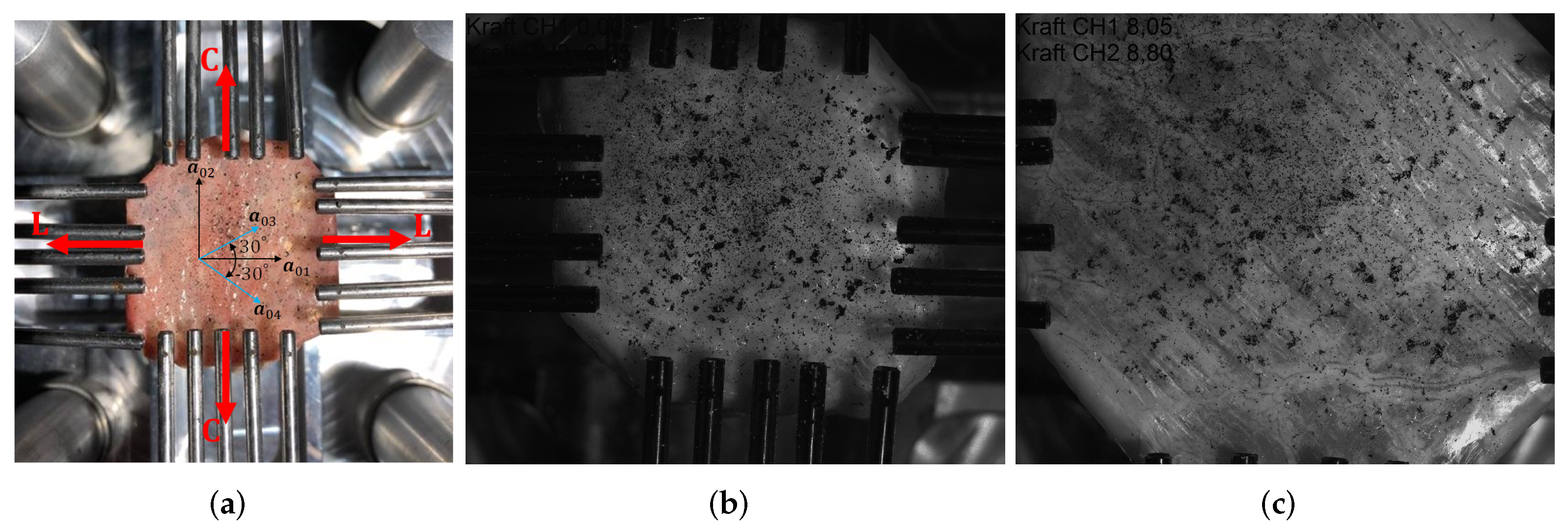
2.1. Preparation of the Equibiaxial Tensile Test Specimens

The large intestine of the pig is removed as a whole organ from the euthanized experimental animals previously used in medical training at the Institute of Laboratory Animal Science at the University Hospital RWTH Aachen and covered with cloths soaked in 0.9% NaCl solution to prevent the tissue from drying out. Within an hour, the lump fresh intestine is brought to the testing facility and divided into segments based on the individual anatomical loops and completely cleaned of feces and other connective/adipose tissue. Each segment is taken in turn and cut lengthwise. Individual samples are cut out with an edge length (L) of 40 mm × 40 mm and stored in a 0.9% NaCl solution preventing desiccation until mechanical testing. The average thickness (0.68 < T < 2.15) of the large intestine is equal to 1.17 mm measured with a micrometer screw prior to testing.

2.2. Test Protocol

The equibiaxial mechanical tests are carried out on a self-developed biaxial tensile testing machine “BiAiX” (FH Aachen, Aachen, Germany, patent pending, DE 10 2017 116 067 A1). For 2D planar evaluation, one Allied Vision Prosilica GT2450, 5 Megapixel camera (Allied Vision Technologies GmbH, Statroda, Germany) with GigE Vision Gigabit Ethernet interface and a maximum frame rate of 15 f/s with AQUAMARINE 2.0/28 C (Schneider Kreuznach, Bad Kreuznach, Germany) lens, is mounted above the BiAiX machine. The two force sensors of the BiAiX tension test machine are calibrated in an industrial manner with calibration weights. The camera is positioned perpendicular to the specimen surface. This guarantees an easy calibration for the 2D DIC with a specified length in the measuring plane. The specimens are then mounted in the apparatus with five needles on each side, taking care to ensure that the orientation of the sample always the same: longitudinal direction along the L-L axis and circumferential direction along the C-C axis (Figure 1a). The needles can move laterally to allow free stretching of each specimen’s side. To ensure a uniform evaluation of the specimens, the inner mucosal layer of the specimens is always oriented facing up and a graphite pattern is sprayed on (Figure 1b) for digital image correlation (DIC). Polarized light with polarizing filters in front of the camera setup was used to avoid any reflections on the specimen. The measurement protocols for the tensile test are as follows: 10 cycles of preconditioning followed by a monotonous stretching both at the speed of 10 mm/min until failure and a framerate of 1 Hz (Figure 1c).

2.3. Virgin Passive Anisotropic Strain Energy Function Description

The strain energy function (SEF) (ψ) of the incompressible anisotropic large intestine can be decomposed into volumetric (${\psi }_{\mathrm{vol}}$), isochoric isotropic (${\overline{\psi }}_{\mathrm{iso}}$) and isochoric anisotropic (${\overline{\psi }}_{\mathrm{aniso}}$) terms [1,24]:

$$\begin{array}{c}\hfill \psi (J,\overline{\mathbf{C}},{\mathbf{a}}_{0i}):={\psi }_{\mathrm{vol}}\left(J\right)+{\overline{\psi }}_{\mathrm{iso}}\left({\overline{I}}_1\right)+\sum _{i=1}^N{\overline{\psi }}_{\mathrm{aniso}}\left({\overline{I}}_{4,{\mathbf{a}}_{0i}}\right),\end{array}$$

(1)

where the Jacobian J = $\det \mathbf{F}$ is the determinant of the deformation gradient F, the isochoric deformation gradient is $\overline{\mathbf{F}}$ = $J^{-1/3}\mathbf{F}$, ${\overline{I}}_1$ = $\mathrm{tr}\overline{\mathbf{C}}$ is the first principal invariant of the isochoric right Cauchy–Green deformation tensor, ($\mathbf{C}$ = ${\overline{\mathbf{F}}}^{\mathrm{T}}\overline{\mathbf{F}}$), ${\mathbf{a}}_{0i}$ = ${\left\{a_{0ix},a_{0iy},a_{0iz}\right\}}^{\mathrm{T}}$ is the unit directional vector of the ith fiber family in the undeformed configuration and ${\overline{I}}_{4,{\mathbf{a}}_{0i}}$ = $\overline{\mathbf{C}}:{\mathbf{A}}_{0i}$ = ${\mathbf{a}}_{0i}\times \overline{\mathbf{C}}·{\mathbf{a}}_{0i}$ includes the anisotropic invariants, which are quantitatively equal to the square of the respective fiber stretches ${\lambda }_{{\mathbf{a}}_{0i}}^2$. At low strain, collagen fibers are not stretched and do not store strain energy. Thus, the tissue mechanical behavior is solely due to the non-collagenous ground matrix and its isotropic response can be defined using the classical Neo-Hookean material model. At large strains, the collagen fibers resist the applied load and show a strong stiffening effect, which can be represented mathematically by an exponential function using the fiber-reinforced hyperelastic Holzapfel–Gasser–Ogden (HGO) model [39]:

$$\begin{array}{cc}\hfill {\psi }_{\mathrm{virgin}\mathrm{passive}}(J,\overline{\mathbf{C}},{\mathbf{a}}_{0i})& =\frac{{\kappa }_0}{2}{\left(J-1\right)}^2+\frac{{\mu }_0}{2}\left({\overline{I}}_1-3\right)\hfill \\ & +\left\{\begin{array}{cc}{\displaystyle \sum _{i=1}^4}\frac{k_{1,{\mathbf{a}}_{0i}}}{2k_{2,{\mathbf{a}}_{0i}}}\left[\exp \left\{k_{2,{\mathbf{a}}_{0i}}{\left({\overline{I}}_{4,{\mathbf{a}}_{0i}}-1\right)}^2\right\}-1\right]\hfill & \mathrm{if}{\overline{I}}_{4{\mathbf{a}}_{0i}}\ge 1\hfill \\ 0\hfill & \mathrm{if}{\overline{I}}_{4{\mathbf{a}}_{0i}}<1\hfill \end{array}\right.,\hfill \end{array}$$

(2)

where ${\kappa }_0>0$ and ${\mu }_0>0$ are the initial bulk and shear moduli, respectively, and have a unit of stress. $k_{1,{\mathbf{a}}_{0i}}>0$ includes stress-like material parameters and $k_{2,{\mathbf{a}}_{0i}}$ involves dimensionless parameters associated with the ith fiber family. It is important to select appropriate $k_1$ and $k_2$ such that the anisotropic isochoric strain energy function induced by the collagen fibers does not influence the overall tissue mechanics at the low strain regime.

2.4. Numerical Simulations

The finite element (FE) analysis has also been performed in the commercial FE software LS-DYNA (Ansys, Inc., Canonsburg, PA, USA) Version: smp d R11.1.0 in 64 bit Windows 10 to validate the estimated material parameters. Although the standard “MAT-295” material model in LS-DYNA is based entirely on the HGO material [39], it is restricted to only three fiber families and is, therefore, not suitable for modeling the intestinal tissue, which is proposed to consist of four collagen fibers (Equation (2)). Therefore, a user-defined FORTRAN material subroutine has been coded inside LS-DYNA.

Two examples are presented in this paper to demonstrate the numerical performance of the implemented user-defined FORTRAN material subroutine using the material parameters estimated from MATLAB’s curve fit. Firstly, a cube of edge length 1 mm meshed with one linear brick element and reinforced by four fiber families (Figure 2a) is considered to validate the basic anisotropic hyperelastic mechanisms of a specific intestine specimen derived from the experiment. The four fiber families are represented by unit directional vectors, ${\mathbf{a}}_{01}$ = ${\left\{100\right\}}^{\mathrm{T}},{\mathbf{a}}_{02}$ = ${\left\{010\right\}}^{\mathrm{T}},{\mathbf{a}}_{03}$ = ${\left\{\cos {30}^{\circ }\sin {30}^{\circ }0\right\}}^{\mathrm{T}}$ and ${\mathbf{a}}_{04}$ = ${\{\cos {30}^{\circ }-\sin {30}^{\circ }0\}}^{\mathrm{T}}$. For equibiaxial tension, the boundary conditions are chosen in such a manner that the four bottom face nodes are constrained to move along the Z-axis, while displacements $\Delta X$ = $\Delta Y$ = 0.3 mm are prescribed on all nodes in the X-Y plane. The fitted material parameters of a specific specimen is to be used. To ensure a nearly incompressible intestine, a large bulk modulus, ${\kappa }_0$ = $5\times {10}^4$ MPa is taken, which provides the initial Poisson’s ratio ${\nu }_0$ = $(3{\kappa }_0-2{\mu }_0)/\left(2(3{\kappa }_0+{\mu }_0)\right)$ = 0.49999999 $\approx 0.5$.

The second example models the biaxial deformation state of an experimented specimen (No. 3,

Table 1. Fitted anisotropic parameters of the porcine large intestine from biaxial tensile experiment data.

Specimen	${\mathit{\mu }}_0$ (MPa)	${\mathit{k}}_{1,\mathbf{Mus}}$ (MPa)	${\mathit{k}}_{2,\mathbf{Mus}}$	${\mathit{k}}_{1,\mathbf{Sm}}$ (MPa)	${\mathit{k}}_{2,\mathbf{Sm}}$	${\mathit{R}}_{\mathbf{L}}^2$	${\mathit{R}}_{\mathbf{C}}^2$
1	0.001	0.0171	1.5827	0.0233	2.4303	0.9900	0.9878
2	0.001	0.0153	0.8525	0.0043	2.5866	0.9968	0.9944
3	0.001	0.0268	0.5080	0.0072	2.0980	0.9924	0.9980
4	0.001	0.0218	1.9014	0.0125	0.9415	0.9873	0.9904
5	0.002	0.0061	0.7490	0.0300	0.4768	0.9798	0.9846
Average curve	0.0048	0.0133	1.2090	0.0136	1.2483	1.0000	1.0000

) with dimension 40 mm × 40 mm × 1.25 mm. Due to the symmetry in geometry and boundary conditions, only a quarter of the model, 20 mm × 20 mm × 1.25 mm, is considered for the numerical analysis (Figure 2b). Compared to the other two dimensions, the intestinal thickness is very small; therefore, only three linear brick elements are taken across the thickness, while thirty linear brick elements are considered along the length and width, maintaining the aspect ratio of 1.6:1 in the undeformed configuration. A total of 2700 linear brick elements are used in this example. The linear brick element is used in this example as well to maintain a consistency in comparing the numerical results in both examples for the same material parameters and the same FORTRAN user subroutine. For the biaxial tension, the bottom face nodes are constrained to move in the Z-axis. The symmetry boundary conditions are imposed to the left face and front face nodes while prescribed displacements are applied to the right face and back face nodes until a desired maximum values.

3. Results

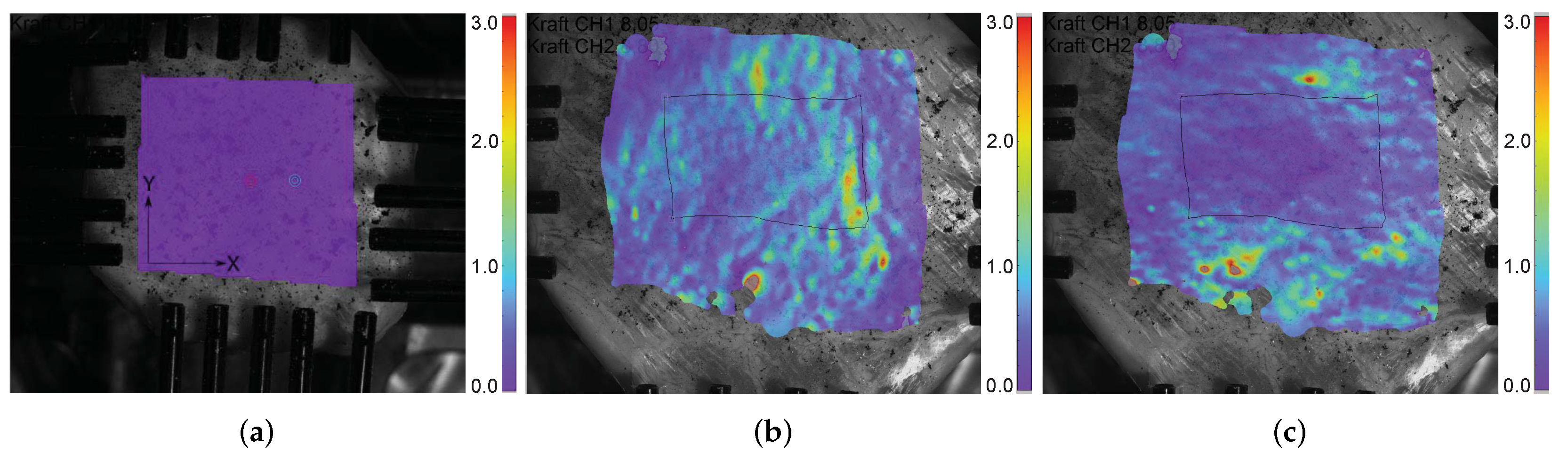
3.1. Equibiaxial Tensile Experiment

Displacement-controlled equibiaxial extension has been applied, which took around 12 min to rupture each specimen. The tractions ($P_i$) are continuously recorded on actuators of longitudinal and circumferential directions at each load step ranging to a maximum value of 8.65–13.75 N and 6.6–15.2 N, respectively. For the DIC evaluation with the ISTRA4D software, residuum = 40–50, facet size > 50 and grid spacing = $\frac{1}{3}$ facet size ≈ 17 are used to obtain a homogeneous strain field without a significant loss of grid points. Most importantly, inhomogenous and anisotropic strain distributions are observed, defined by several in-plane ripples that looks similarly to calm ocean waves directed vertically for the X-axis and horizontally for the Y-axis (Figure 3b,c). No concrete evidence can be found where the underlying collagen fibers withstood the stress. However, a higher magnification and higher resolution camera, if available, may be utilized to resolve such strain distributions.

3.2. Intestinal Anisotropy

As shown in Figure 4, the equibiaxially stretched porcine large intestine is stiffer in the longitudinal direction than in the circumferential direction: the additional stiffness is provided by thicker submucosal collagen fibers (${\mathbf{a}}_{03},{\mathbf{a}}_{04}$). Feng et al. [40] used the second harmonic generation and measured the diameters of the load bearing collagen fibers in the large intestine. The largest (≈6.5 μm) is found in the submucosal layer and the smallest, ≈1.9 μm, is found in the muscularis layer. The non-interacting collagen fibers in the longitudinal and the circumferential muscular layers are orthogonal, i.e., ${\alpha }_{\mathrm{Mus}}$ = ${\cos }^{-1}\left({\mathbf{a}}_{01}·{\mathbf{a}}_{02}\right)$ = ${90}^{\circ }$. However, the submucosal collagen fibers are oriented crosswise at an angle of ${\alpha }_{\mathrm{Sm}}$ = ${\cos }^{-1}\left({\mathbf{a}}_{03}·{\mathbf{a}}_{04}\right) \approx \pm {30}^{\circ }$ to the longitudinal direction, ignoring the possible interactions between these fibers in this study. Assuming that the collagen fiber diameters in the longitudinal and the circumferential muscular layer are the same, one isotropic (${\mu }_0$) and four anisotropic material parameters ($k_{i,{\mathbf{a}}_{01}}$ = $k_{i{\mathbf{a}}_{02}}$ = $k_{i,\mathrm{Mus}}$ and $k_{i,{\mathbf{a}}_{03}}$ = $k_{i,{\mathbf{a}}_{04}}$ = $k_{i,\mathrm{Sm}},\forall i$ = $1,2$) are to be estimated to fit the experimental stress–strain curves. For this systematic characterization of the virgin passive anisotropy of the porcine large intestine (Equation (2)), only five parameters are sufficient to fit the experimental Cauchy stress–stretch data. For this, the Green–Lagrange strains ($E_{ii}$) in both loading directions are evaluated directly from the heat maps (Figure 3) using the DIC technique in the ISTRA 4D (Limess Messtechnik und Software GmbH, Krefeld, Germany) software for each individual images and are recorded as an averaged value from a chosen deformation region (Figure 3). From the Lagrangian strain and using the incompressibility condition, the true or Cauchy stress (${\sigma }_{ii}$ = $P_i{\lambda }_i/LT$) is set as a function of the elongation (${\lambda }_i$ = $\sqrt{2E_{ii}+1}$) and curve fitting is performed in MATLAB (The MathWorks, Inc., Natick, MA, USA) on the basis of a non-linear least-squares optimization method to determine the passive incompressible anisotropic material parameters per SEF described in Section 2.3. The fitted curves are shown in Figure 4, for which the estimated parameters are listed in Table 1. The quality of the fitting is measured by calculating the coefficient of determination $R^2\in \left[0,1\right]$ in the longitudinal ($R_{\mathrm{L}}^2$) and circumferential ($R_{\mathrm{C}}^2$) directions, respectively, using the following:

$$\begin{array}{c}\hfill R^2=1-\frac{{\displaystyle \sum _{i=1}^n}{\left({\sigma }_i^{\exp }-{\sigma }_i^{\mathrm{fit}}\right)}^2}{{\displaystyle \sum _{i=1}^n}{\left({\sigma }_i^{\exp }-{\sigma }^{\mathrm{mean}}\right)}^2}.\end{array}$$

(3)

where n is the number of measured data points, ${\sigma }_i^{\exp }$ is the Cauchy stress measured experimentally, ${\sigma }_i^{\mathrm{fit}}$ is the corresponding stress values predicted by the fitting procedure using the SEF and ${\sigma }^{\mathrm{mean}}$ is the mean of the experimental stress. The higher the value of $R^2$, the better the fit is to predict the experimental data.

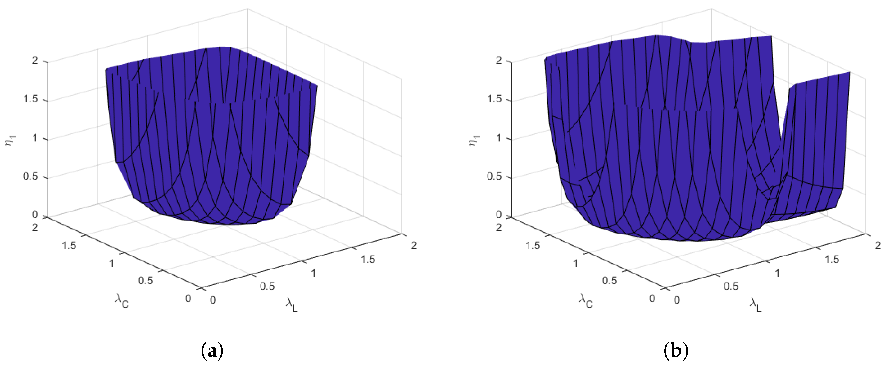
3.3. Parameter Stability

The estimated virgin passive anisotropic parameters (Table 1) are to be fed in the FE software for the numerical simulation and, thus, need to be numerically stable, fulfilling the polyconvexity of the SEF. Unstable parameters and non-convex SEF may lead to unphysical behavior during large deformations [41]. Convexity of the SEF in Equation (2) guarantees the existence of at least one local minimum energy state for which the eigenvalues ${\eta }_{1,2}$ = $\frac{1}{2}[(H_{11}+H_{22})\pm \sqrt{{(H_{11}-H_{22})}^2+4H_{12}^2}]$ of the planar Hessian matrix ($H_{ij}$ = ${\partial }^2{\psi }_{\mathrm{virgin}\mathrm{passive}}/\partial {\lambda }_i\partial {\lambda }_j,\forall i,j$ = $1,2$) need to be positive [42,43]. Positive eigenvalues render the Hessian matrix positive definite and the SEF convex at every point in the strain space results in a positive definite elasticity tensor or a positive definite stiffness matrix that guarantees stable material parameters. For thin specimens with homogeneous plane biaxial stress and deformation states, only two components are sufficient because the third principal stress is zero. The numerical stability of the fitted parameters for the virgin passive deformation state (Figure 5) can be verified by plotting the positive three dimensional surfaces of the eigenvalues (${\eta }_1,{\eta }_2$) as the function of biaxial stretch (${\lambda }_{\mathrm{L}},{\lambda }_{\mathrm{C}}$) (see Figure 5).

3.4. Numerical Simulations

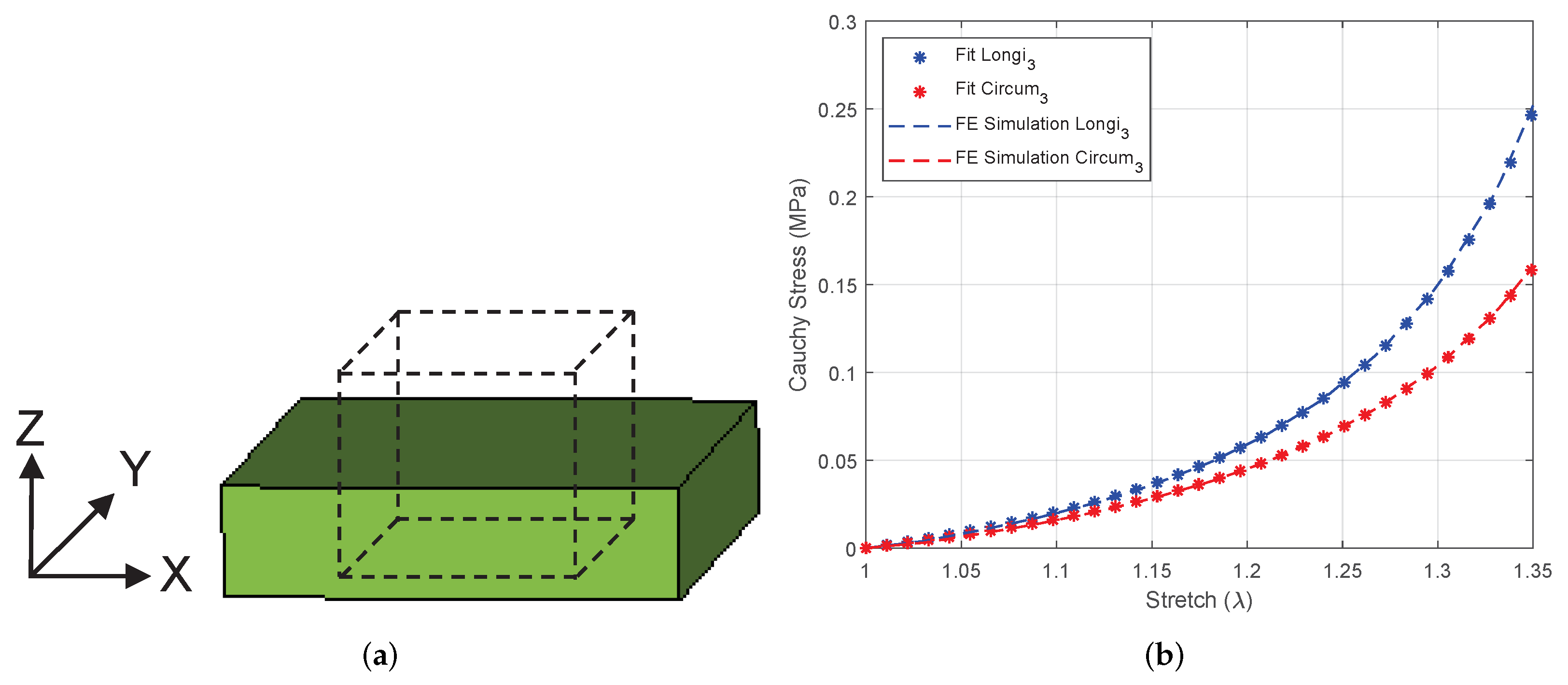
3.4.1. Equibiaxial Tension of a Linear Brick Element

The equibiaxial stretch simulation result of the linear brick element is shown in Figure 6. Due to the prescribed elongations ($\Delta X$ = $\Delta Y$ = 0.3 mm) along the X and the Y axis, the brick model is compressed ($\Delta Z=-0.61$ mm) along the Z axis (Figure 6a). The Cauchy stress and the strain data in the linear element along the longitudinal (X-axis) and the circumferential (Y-axis) directions are extracted from LS-PrePost. The respective stretches in both directions are computed and the Cauchy stress vs. stretch curves are plotted over the fit dataset. From the simulation, a clear anisotropy has been achieved with a longitudinal stiffness larger than the circumferential direction. Furthermore, the material behavior is exactly same as the dataset that characterizes the chosen specimen No. 3 during the equibiaxial tensile experiment. This would confirm that the (a) materials with the estimated material parameters are numerically stable and (b) the implemented FORTRAN user material subroutine is capable for further numerical investigations; as presented in Section 3.4.2.

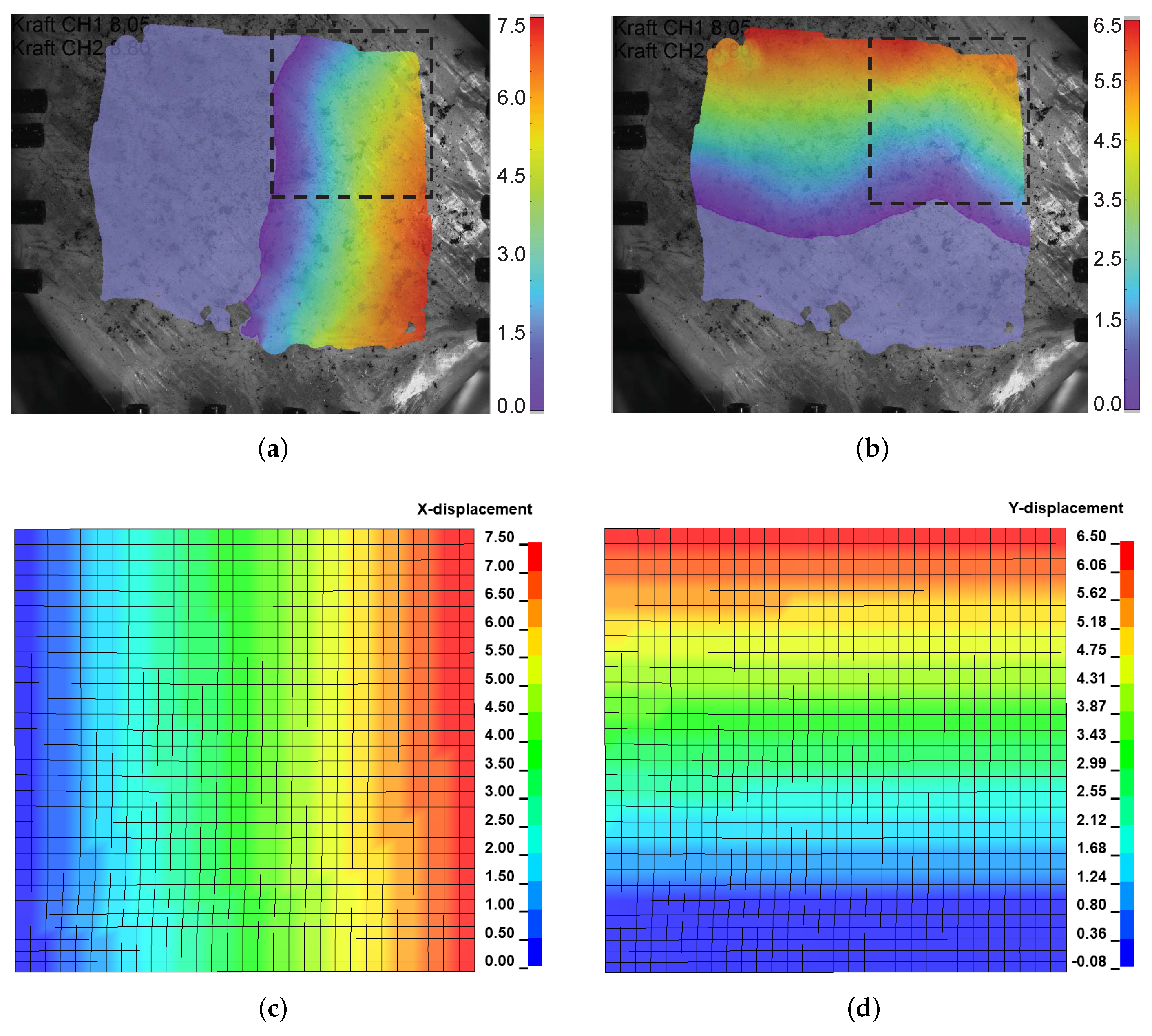
3.4.2. Equibiaxial Tension of an Intestine Specimen

Figure 7a,b show the displacements of specimen No. 3 measured with DIC during the biaxial tensile test along the longitudinal and the circumferential directions, respectively. The displacements are measured with DIC and plotted in one-half of the specimen to compare the result with the computer simulation. The linear brick element has also been used in this example because the results of the first example using this element are objectively accurate for predicting the large deformation of the intestine tissue material. The equibiaxial tension simulation of the tested specimen No. 3 has been performed taking into account the geometric and loading symmetries for which the total simulation time took around 7 min using 16 CPUs. The results of the biaxial extensions of the corresponding computer model along both directions are shown in Figure 7c,d. The contours of the displacements from the FE simulation are quantitatively and qualitatively mapable to that observed in the DIC images from the experiment (Figure 7a,b).

Thus, the implemented user subroutine tool is satisfactorily able to predict the virgin passive mechanical behavior of the multi-layered intestine tissue and similar architecture, provided that the estimated material parameters for the adopted HGO model are numerically stable. However, the physiological response of the in vivo intestine is not limited to virgin passive hyperelastic anisotropy. Intestinal peristalsis due to continuous smooth muscle contraction–relaxation, viscoelasticity due to water content and damage either due to tissue remodeling, growth or injuries are other important aspects of colon biomechanics. Since the damage modeling intestine tissues has not been studied before, the authors would like to review some of the existing literature on (a) the concept of intestinal peristalsis and (b) various constitutive models for smooth muscle contraction and the viscoelasticity of the colorectal tissues.

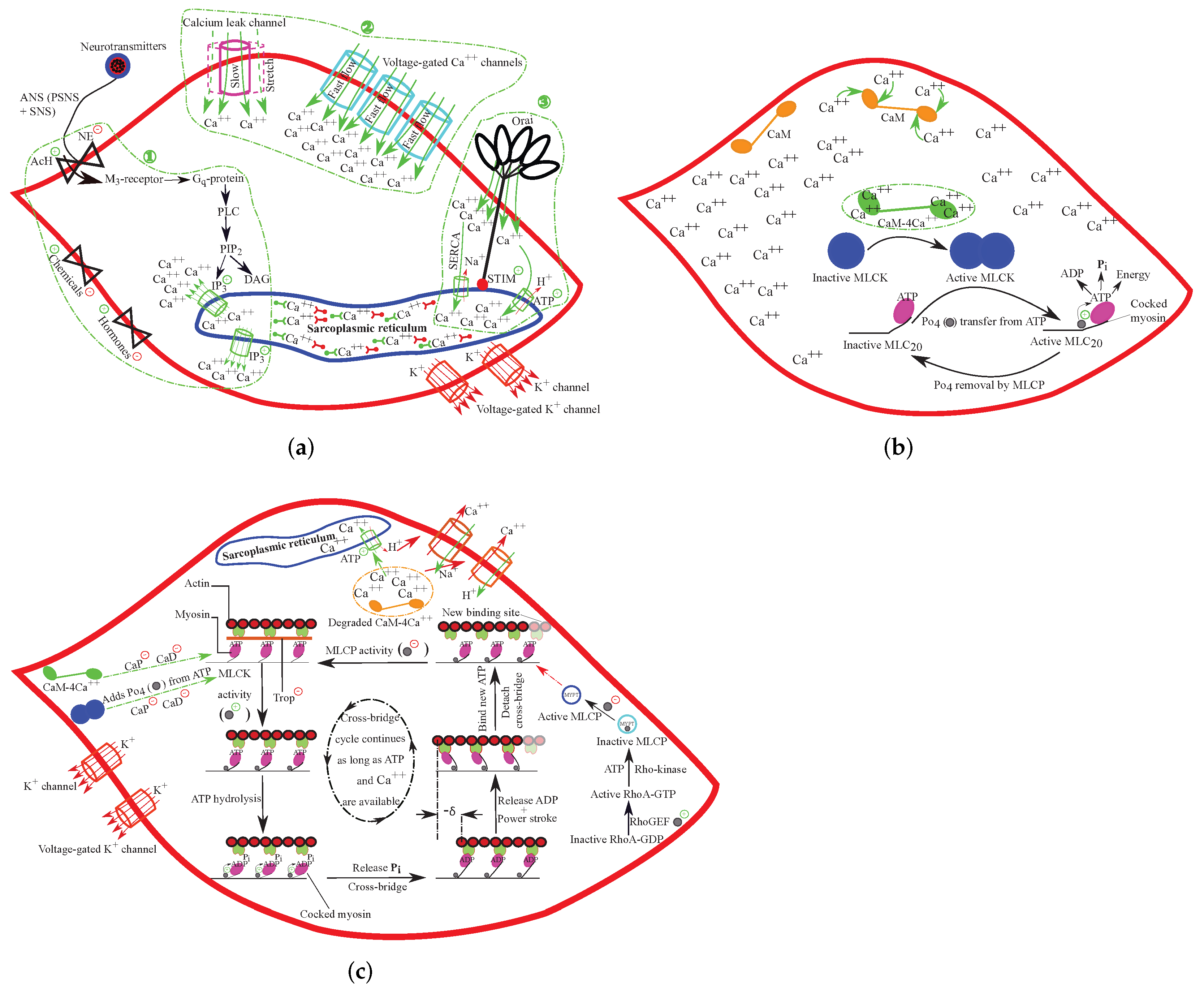
4. Physiology of Intestinal Peristalsis

The colonic motility or peristalsis is characterized by the coordinated contraction–relaxation of longitudinal and circular smooth muscle cells (SMCs) regulated by the enteric and the parasympathetic nervous system [44,45,46]. On an anatomical level, during peristaltic propulsion, the circular SMCs behind fecal content contract and relax in the receiving segment, whereas longitudinal SMCs relax behind the luminal content and contract in the front (Figure 8). The luminal cross-section in the receiving segment widens to facilitate the forward-movement of the intraluminal content [47]. On the electrical level, the smooth muscle contraction–relaxation is driven by an excitatory-inhibitory response of an electrically coupled multi-cellular SMC/ICC/PDGFRα⁺ cell syncytium (SIP syncytium) connected via gap junctions [48]. Innervated with excitatory enteric motor neurons, the interstitial cells of Cajal (ICC) stimulate unique Ca⁺⁺-activated Cl⁻ channels or K⁺ channels and generate excitatory electrical slow waves or currents to enhance SIP syncytium excitability and to initiate the rapid contraction of SMCs [49,50]. In contrast, platelet-derived growth factor receptor α-positive (PDGFRα⁺), the inhibitory neurotransmitter released from enteric motor neurons, expresses small conductance calcium-activated K⁺ channel 3 (Ca⁺⁺-activated SK3) channel to generate inhibitory currents, thereby reducing SIP syncytium excitability and reducing SMC contraction [49,51]. Most importantly, the level of free cytoplasmic or intracellular Ca⁺⁺ within SMC determines its cellular contraction–relaxation activity. In response to a slow influx of Ca⁺⁺ through leak channels, acetylcholine (AcH) neurotransmitter, H⁺, hormones, sarcoplasmic reticulum calcium spark, the stimulation of voltage-gated Ca⁺⁺ channels, ATPase, sacro/endoplasmic reticulum Ca⁺⁺ ATPase (SERCA), stromal interaction molecule (STIM) protein and Orai protein activities rapidly increase Ca⁺⁺ concentrations. Such processes are schematically shown by three green-dashed regions in Figure 9a. In any such cases, enhanced SMC contraction is depicted by a rapid spike of the membrane potential, known as action potential well above the threshold potential, which is counteracted by repolarization, i.e., outflow of K⁺ ions from the activated K⁺ channels (Figure 9a).

On the molecular level, smooth muscle contraction–relaxation is regulated by the opposing activity of the myosin light chain kinase (MLCK) and myosin light chain phosphatase (MLCP), thereby modulating the phosphorylation of 20 kDa regulatory light chain of myosin II (MLC20) [52,53]:The latter is Ca⁺⁺ independent. Triggered by inositol 1,4,5-trisphosphate (IP3), Ca⁺⁺ activates the enzymatic domain of MLCK, which is mediated by the calmodulin (CaM) via CaM-4Ca⁺⁺-dependent complex formation (Figure 9b). This CaM-4Ca⁺⁺ complex phosphorylates the Ser19 hydroxyl group at the neck of MLC20 to stimulate myosin Adenosine tri-phosphate (ATP) hydrolysis into Adenosine di-phosphate (ADP), inorganic phosphate (${\mathbf{P}}_{\mathrm{i}}$) and energy at its globular head. The inhibition of tropomyosin (Trop), calponin (CaP) and caldesmon (CaD) followed by the release of ${\mathbf{P}}_{\mathrm{i}}$ from the myosin head exposes the myosin binding sites to initiate myosin–actin cross bridging (Figure 9c). Powered by the chemical energy stored in the myosin’s head, actin–myosin slide over one another with the release of ADP to shorten the length between two dense bodies by $-\delta$. Sliding continues until a new ATP molecule is attached to the myosin head, which immediately detaches the myosin from the actin binding sites. At the end of this cycle, Ca⁺⁺-independent MLCP dephosphorylates MLC20 [52] and inhibits CaM-4Ca⁺⁺-activated ATPase activity [53]. Furthermore, the kinases from cyclic nucleotides inhibit incoming Ca⁺⁺ channel activities, phosphorylate MLCK to reduce its affinity for the activated CaM-4Ca⁺⁺ complex and finally decrease myosin phosphorylation [54]. Furthermore, they may stimulate Ca⁺⁺ uptake from the CaM-4Ca⁺⁺ complex and the cytosol to the sarcoplasmic reticulum and outside the SMC through Ca⁺⁺/Na⁺ or Ca⁺⁺/H⁺ exchanges (Figure 9c). Thus, reduced intracellular CaM-4Ca⁺⁺ MLCK activity and increased MLCP activity relaxes SMCs.

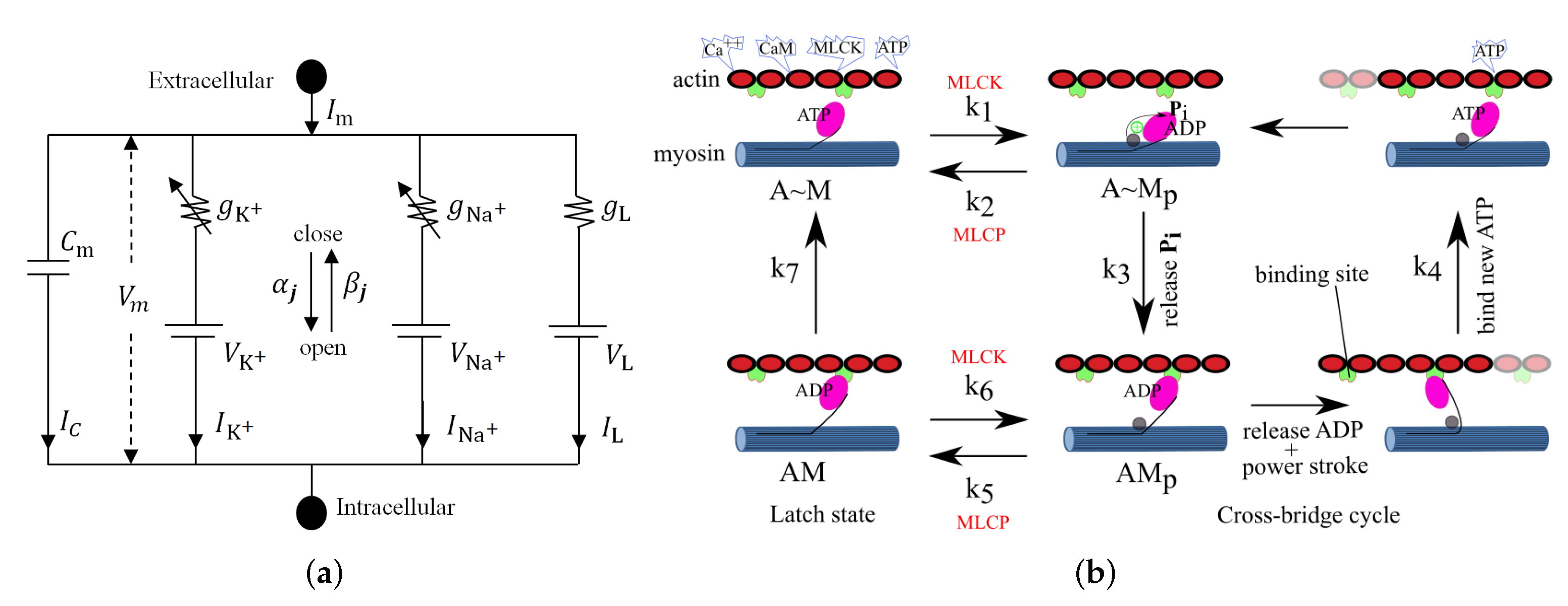
5. Constitutive Modeling of Large Intestinal SMC Contraction

In most of the available mechanical characterizations and computational studies of the intestine tissue, the tonic active contraction of the SMCs has been ignored [1]. The mechanical description of the contraction of SMCs qualitatively resembles skeletal muscles [55] and cardiac muscles [56,57]; however, SMCs differ from skeletal muscles in having a longer contraction time at a much slower rate. Myosin ATP hydrolysis provides chemical energy to produce cyclic cross-bridges between actin and myosin filaments and to generate a power stroke to result tonic and phasic SMC (Figure 9). HE Huxley, the nobel laureates AV Hill and AF Huxley and their co-authors pioneered the conceptualization of skeletal muscle contraction, and this formulation is applicable to SMCs as well [58].

The existing muscle models are conceptually based on the three-element muscle model [59] and the sliding-filament hypothesis [60,61,62]. SMC mechanics have been estimated by a system of ordinary differential equations (ODEs) based on the electrical, chemical and mechanical processes involved. The electrochemical process involves a regulation of the intracellular Ca⁺⁺ concentration due to stimulated nerve action potential for which the conductance-based model by Hodgkin–Huxley is useful [63,64]. The voltage-dependent K⁺ and Na⁺ ion channels (action potential) and leakage (L) ion channel (small conductance for resting membrane potential) are regulated by small gates in the intestinal SMCs. Membrane potentials higher than the threshold potential open the Na⁺ channel to depolarize the membrane and to activate voltage-gated Ca⁺⁺ channel for rapid inflow, followed by a rapid spike or action potential and the contraction. In a voltage clamp set up (Figure 10a), the Hodgkin–Huxley model uses electric circuit relationships and ODEs to measure ion currents ($I_i$) through each ion channels (i = ${\mathrm{K}}^{+},{\mathrm{Na}}^{+},\mathrm{L}$) and compares the input/output currents at a desired membrane potential ($V_m$) at any time t:

$$\begin{array}{cc}\hfill I_m\left(t\right)& =I_{\mathrm{C}}\left(t\right)+\sum _i{I}_i\left(t\right)\hfill \\ \hfill & =C_m\frac{d{V}_m}{dt}+g_{{\mathrm{K}}^{+}}{n}^4\left(V_m-V_{{\mathrm{K}}^{+}}\right)+g_{{\mathrm{Na}}^{+}}{m}^{3}h\left(V_m-V_{{\mathrm{Na}}^{+}}\right)+g_L\left(V_m-V_L\right)\hfill \\ \hfill \frac{dn}{dt}& ={\alpha }_n\left(V_m\right)\left(1-n\right)-{\beta }_n\left(V_m\right)n\hfill \\ \hfill \frac{dm}{dt}& ={\alpha }_m\left(V_m\right)\left(1-m\right)-{\beta }_m\left(V_m\right)m\hfill \\ \hfill \frac{dh}{dt}& ={\alpha }_h\left(V_m\right)\left(1-h\right)-{\beta }_h\left(V_m\right)h,\hfill \end{array}$$

(4)

where $I_m$ is the input current flowing into the membrane; $I_{\mathrm{C}}$ is the capacity current associated with the membrane capacitor $C_m$ that stores the imbalanced positive–negative membrane current; $V_i\ne V_m$ and $g_i$ are the ith ion channel reversal potentials and respective maximum values of conductance per unit area; $n,m$ and $h\in [0,1]$ are dimensionless gating variables that are associated with K${}^{+}$ channel activation (gate opened), Na${}^{+}$ channel activation (gate opened) and Na${}^{+}$ channel inactivation (gate closed) with the powers in Equation (5) representing the number of gates used. ${\alpha }_i$ and ${\beta }_i$ are the voltage-dependent transition rate constants for the ith ion channels, where ${\alpha }_i$ is the number of times per second that a closed gate opens and ${\beta }_i$ is the number of times per second that a opened gate closes. These rates for stretch-sensitive colorectal afferent endings are expressed by Feng et al. [64].

$$\begin{array}{cccc}\hfill {\alpha }_n& =0.1\left(\frac{V+52}{12.5}\right){\left[1-\exp \left(-\frac{V+52}{12.5}\right)\right]}^{-1};\hfill & \hfill & {\beta }_n=0.125\exp \left(-\frac{V+60}{80}\right)\hfill \\ \hfill {\alpha }_m& =1.548{\left[1+\exp \left(-\frac{V-11.01}{14.871}\right)\right]}^{-1};\hfill & \hfill & {\beta }_m=8.685{\left[1+\exp \left(\frac{V+112.4}{22.9}\right)\right]}^{-1}\hfill \\ \hfill {\alpha }_h& =0.2574{\left[1+\exp \left(\frac{V+63.264}{3.7193}\right)\right]}^{-1};\hfill & \hfill & {\beta }_h=0.53984{\left[1+\exp \left(-\frac{V-0.27853}{9.0933}\right)\right]}^{-1}.\hfill \end{array}$$

(5)

Hai and Murphy conducted chemomechanical setups and proposed a four-state cross-bridge chemical kinetic model [65] depending on the chemical states of myosin (Figure 10b): actin detached unphosphorylated myosin (A∼M), actin detached phosphorylated myosin (A∼M_p), actin attached phosphorylated myosin (AM_p), also known as cross bridge, and actin attached unphosphorylated myosin (AM), also known as latch bridge. The model is governed by a first-order differential equations system:

$$\begin{array}{c}\hfill \frac{d}{dt}\left(\begin{array}{c}{n}_1\\ n_2\\ n_3\\ n_4\end{array}\right)=\left[\begin{array}{cccc}-k_1& k_2& 0& k_7\\ k_1& -k_2-k_3& k_4& 0\\ 0& k_3& -k_4-k_5& k_6\\ 0& 0& k_5& k_6-k_7\end{array}\right]\left(\begin{array}{c}{n}_1\\ n_2\\ n_3\\ n_4\end{array}\right),\end{array}$$

(6)

with an additional constraint on the population fraction ($n_i$) of myosin heads in each state, $n_1$(A∼M) + $n_2$(A∼M_p) + $n_3$(AM_p) + $n_4$(AM) = 1. This means that the total sum of the myosin fraction must remain constant. Here, ($k_1,k_6$) are the position-independent state transition rates of myosin phosphorylation, ($k_2,k_5$) are the position-independent rates of myosin dephosphorylation, ($k_4,k_7$) and ($k_3$) are the position-dependent rates for myosin detachment and attachment, respectively. The interesting aspects of this models are as follows: (a) $k_1$ and $k_6$ are regulated by Ca⁺⁺ concentrations and (b) AM→A∼M is irreversible. Furthermore, a hyperbolic dependency of steady-state active stress on cross-bridge phosphorylation [65] and a direct correlation of myosin phosphorylation relative to the force generation and tissue shortening velocity have been found [66]. Singer et al. [67] further supported the Ca⁺⁺-dependent latch bridged mechanical differences with phosphorylated cross-bridges and decomposed the total SMCs stress into active and passive stress: the latter by depleting extracellular Ca⁺⁺. Kato et al. [68] followed Hai and Murphy and proposed a kinetic model to correlate the CaM-4Ca⁺⁺-dependent activation of MLCK, the phosphorylation–dephosphorylation of myosin and isometric contractions in SMC at a steady state.

Based on the four-state cross-bridge chemical kinetic model by Hai and Murphy, the active contraction of the guinea pig taenia coli SMC under large deformation has been proposed by Kroon [69]. The calcium-regulated active chemical response is due to the contractile apparatus consisting of elastic spring (cross-bridges stiffness) and a dashpot (relative sliding between actin and myosin) in parallel with the passive viscoelastic combination and is mathematically expressed as follows:

$$\begin{array}{c}\hfill {\psi }_{\mathrm{act}}=\frac{{\mu }_{\mathrm{f}}}{4}\left(n_3+n_4\right){\left({\lambda }_{\mathrm{e}}^2-1\right)}^2=\frac{{\mu }_{\mathrm{f}}}{4}\left(n_3+n_4\right){\left(\frac{\mathbf{MCM}}{{\lambda }_{\mathrm{fc}}^2}-1\right)}^2,\end{array}$$

(7)

where ${\psi }_{\mathrm{act}}$ is the active part of SEF, ${\mu }_{\mathrm{f}}$ is related to the stiffness of the cross-bridges and the number of myosin and actin filaments per unit area, ($n_3+n_4$) is the fraction of cross-bridges contributing to the filament stiffness, M is the direction vector of the contractile filaments in the undeformed configuration, C is the right Cauchy–Green deformation, ${\lambda }_{\mathrm{e}}$ = ${\lambda }_{\mathrm{f}}/{\lambda }_{\mathrm{fc}}$ is the elastic stretching of the cross-bridges, ${\lambda }_{\mathrm{fc}}$ is the relative sliding between contractile filaments and ${\lambda }_{\mathrm{f}}^2$ = $\mathbf{MCM}$ is the tissue stretch along the contractile filament direction. The evolution of ${\lambda }_{\mathrm{fc}}$ is adopted as $\eta {\dot{\lambda }}_{\mathrm{fc}}$ = $P_{\mathrm{cc}}-tial{\psi }_{\mathrm{act}}/tial{\lambda }_{\mathrm{fc}}$, where η is the viscous damping coefficient associated with the cycling/contraction process and $P_{\mathrm{cc}}$ is the active stress due to attached cross-bridges causing muscle contraction. The process of the filament contraction development in AM_p AM states can be accounted for by an active stress formulation:

$$\begin{array}{c}\hfill P_{\mathrm{cc}}=\left\{\begin{array}{cc}-{\kappa }_3{n}_3\hfill & \mathrm{for}{\kappa }_3{n}_3\ge -\frac{tial{\psi }_{\mathrm{act}}}{tial{\lambda }_{\mathrm{fc}}}>{\kappa }_3{n}_3+{\kappa }_4{n}_4\hfill \\ \frac{tial{\psi }_{\mathrm{act}}}{tial{\lambda }_{\mathrm{fc}}}\hfill & \mathrm{for}{\kappa }_3{n}_3<-\frac{tial{\psi }_{\mathrm{act}}}{tial{\lambda }_{\mathrm{fc}}}\le {\kappa }_3{n}_3+{\kappa }_4{n}_4\hfill \end{array}\right.,\end{array}$$

(8)

where ${\kappa }_3$ and ${\kappa }_4$ are the material parameters related to the driving force of cross-bridges in state AM_p and passive resisting strength of cross-bridges in state AM, respectively. To model taenia coli SMCs, ${\mu }_{\mathrm{f}}$ = ${\kappa }_3$ = 1.11 MPa, ${\kappa }_4$ = 0 (for monotonic contraction with inactive latch state) and η = 44.5 MPa, $k_1$ = $k_6$ = $0.17{\mathrm{s}}^{-1},k_2$ = $k_5$ = $0.5{\mathrm{s}}^{-1},k_3$ = $4k_4,k_4$ = $0.11{\mathrm{s}}^{-1}$ and $k_7$ = $0.01{\mathrm{s}}^{-1}$ have been used for both isotonic and isometric behavior with an increase in Ca⁺⁺ = 2.5 mol/m³ [69].

Likewise, an anisotropic visco-hyperelastic formulation has been proposed by Gizzi and Pandolfi [70] to model the colon visco-electro-active response and the interaction of slow waves (electrical control activity) and fast waves (electrical response activity). The electrodynamics of the intestinal longitudinal muscular (LM) and the ICC (I) layers, i.e., dimensionless transmembrane potentials ($u_{\mathrm{LM}},u_{\mathrm{I}}$) and slow transmembrane currents ($v_{\mathrm{LM}},v_{\mathrm{I}}$) are defined using a pair of partial differential equations per layer:

$$\begin{array}{cc}\hfill & tia{l}_t{u}_{\mathrm{LM}}=f\left(u_{\mathrm{LM}}\right)+D_{\mathrm{LM}}{\nabla }^2{u}_{\mathrm{LM}}-v_{\mathrm{LM}}+F_{\mathrm{LM}}(u_{\mathrm{LM}},u_{\mathrm{I}})\hfill \\ \hfill & tia{l}_t{v}_{\mathrm{LM}}={ϵ}_{\mathrm{LM}}[{\gamma }_{\mathrm{LM}}(u_{\mathrm{LM}}-{\beta }_{\mathrm{LM}})-v_{\mathrm{LM}}]\hfill \\ \hfill & tia{l}_t{u}_{\mathrm{I}}=g\left(u_{\mathrm{I}}\right)+D_{\mathrm{I}}{\nabla }^2{u}_{\mathrm{I}}-v_{\mathrm{I}}+F_{\mathrm{I}}(u_{\mathrm{LM}},u_{\mathrm{I}})\hfill \\ \hfill & tia{l}_t{v}_{\mathrm{I}}={ϵ}_{\mathrm{I}}\left(z\right)[{\gamma }_{\mathrm{I}}(u_{\mathrm{I}}-{\beta }_{\mathrm{I}})-v_{\mathrm{I}}]\hfill \\ \hfill & f\left(u_{\mathrm{LM}}\right)=k_{\mathrm{LM}}{u}_{\mathrm{LM}}(u_{\mathrm{LM}}-a_{\mathrm{LM}})(1-u_{\mathrm{LM}}),F_{\mathrm{LM}}(u_{\mathrm{LM}},u_{\mathrm{I}})={\alpha }_{\mathrm{LM}}{D}_{\mathrm{LM},\mathrm{I}}(u_{\mathrm{LM}}-u_{\mathrm{I}})\hfill \\ \hfill & g\left(u_{\mathrm{I}}\right)=k_{\mathrm{I}}{u}_{\mathrm{I}}(u_{\mathrm{I}}-a_{\mathrm{I}})(1-u_{\mathrm{I}}),F_{\mathrm{I}}(u_{\mathrm{LM}},u_{\mathrm{I}})={\alpha }_{\mathrm{LM}}{D}_{\mathrm{I},\mathrm{LM}}(u_{\mathrm{LM}}-u_{\mathrm{I}}),\hfill \end{array}$$

(9)

where $u_{\mathrm{LM}},u_{\mathrm{I}}$ can be computed using the dimensional transmembrane potentials ($V_{\mathrm{LM}},V_{\mathrm{I}}$).

$$\begin{array}{c}\hfill u_{\mathrm{LM}}=\frac{V_{\mathrm{LM}}-V_{\mathrm{LM},\min }}{V_{\mathrm{LM},\max }-V_{\mathrm{LM},\min }};u_{\mathrm{I}}=\frac{V_{\mathrm{I}}-V_{\mathrm{I},\min }}{V_{\mathrm{I},\max }-V_{\mathrm{I},\min }}.\end{array}$$

(10)

For more information on $f\left(u_{\mathrm{LM}}\right),g\left(u_{\mathrm{I}}\right),{\beta }_{\mathrm{LM}},{\beta }_{\mathrm{I}},{\gamma }_{\mathrm{LM}},{\gamma }_{\mathrm{I}},F_{\mathrm{LM}}(u_{\mathrm{LM}},u_{\mathrm{I}}),F_{\mathrm{I}}(u_{\mathrm{LM}},u_{\mathrm{I}}),D_{\mathrm{LM}},$$D_{\mathrm{I}},D_{\mathrm{LM},\mathrm{I}},D_{\mathrm{I},\mathrm{LM}}$, readers may refer to [70] and the values of the parameters are provided in I of

Table 2. Parameters for the porcine intestine [70].

I Electrical-chemical-mechanical constitutive parameters. Units in cm, s

LM:

$k_{\mathrm{LM}}$ = 10

$a_{\mathrm{LM}}$ = $0.06$

${\beta }_{\mathrm{LM}}$ = 0

${\gamma }_{\mathrm{LM}}$ = 8

${ϵ}_{\mathrm{LM}}$ = $0.15$

${\alpha }_{\mathrm{LM}}$ = 1

ICC:

$k_{\mathrm{I}}$ = 7

$a_{\mathrm{I}}$ = $0.5$

${\beta }_{\mathrm{I}}$ = $0.5$

${\gamma }_{\mathrm{I}}$ = 8

${ϵ}_{\mathrm{I}}$ = ${ϵ}_{\mathrm{I}}\left(z\right)$

${\alpha }_{\mathrm{I}}$ = $-1$

LM:

$D_{\mathrm{LM},\mathrm{I}}$ = $0.3$

$D_{\mathrm{LM}}$ = $0.4$

ICC:

$D_{\mathrm{I},\mathrm{LM}}$ = $0.3$

$D_{\mathrm{I}}$ = $0.04$

II Viscoelastic-active electromechanical model parameters

${\kappa }_0$

${\mu }_1$

${\mu }_2$

$k_{1,{\mathbf{a}}_1}$

$k_{2,{\mathbf{a}}_1}$

$k_{1,{\mathbf{a}}_2}$

$k_{2,{\mathbf{a}}_2}$

$\zeta$

$\eta$

${\chi }_{\mathrm{iso}}$

${\chi }_{\mathrm{fiber}}$

${\chi }_{\mathrm{iso}}^{\mathbf{C}}$

${\chi }_{\mathrm{fiber}}^{\mathbf{C}}$

kPa

kPa

kPa

kPa

-

kPa

-

kPa s

kPa s

-

-

-

-

5.5

1

1

55

56

20

29

0.125

0.09

1

5

3

12

${ϵ}_0$ is the vacuum permittivity or the absolute dielectric permittivity of the vacuum. Its value is not specifically provided in [70]; however, it may be taken as 8.854 × 10⁻¹² Farads per meter.

. The excitability parameter ${ϵ}_{\mathrm{I}}$ is a function of the distance from pylorus (z-axis) that has been approximated from experiments with the following expression.

$$\begin{array}{c}\hfill {ϵ}_{\mathrm{I}}\left(z\right)=0.032+0.05\exp \left(\frac{z}{68}\right).\end{array}$$

(11)

6. Intestinal Active Viscoelasticity

Furthermore, Gizzi et al. [70] extended the SMCs in anisotropic tissue with two preferential directions ${\mathbf{a}}_1$ and ${\mathbf{a}}_2$ to describe the viscoelasticity of the intestine, and SEF takes the following form:

$$\begin{array}{c}\hfill \psi ={\psi }_{\mathrm{elas}}({\mathbf{F}}_{\mathrm{elas}},{\mathbf{a}}_1,{\mathbf{a}}_2)+{\psi }_{\mathrm{act}}(\mathbf{F},\mathbf{E},{\mathbf{a}}_1,{\mathbf{a}}_2)+{\psi }_{\mathrm{visc}}\left(\mathbf{F}\right),\end{array}$$

(12)

where the elastic (${\psi }_{\mathrm{elas}}$), viscous (${\psi }_{\mathrm{visc}}$) and active (${\psi }_{\mathrm{act}}$) SEF are expressed as follows:

$$\begin{array}{cc}\hfill & {\psi }_{\mathrm{elas}}=\frac{1}{2}{\kappa }_0{J}_{\mathrm{elas}}^2+{\mu }_1\left({\overline{I}}_{1,\mathrm{elas}}-3\right)+{\mu }_2\left({\overline{I}}_{2,\mathrm{elas}}-3\right)+\sum _{i=1}^2\frac{k_{1,{\mathbf{a}}_i}}{k_{2,{\mathbf{a}}_i}}\exp \left\{k_{2,{\mathbf{a}}_i}{\left({\overline{I}}_{4,{\mathbf{a}}_i,\mathrm{elas}}-1\right)}^2-1\right\};\hfill \\ \hfill & {\psi }_{\mathrm{visc}}=J\left[\frac{1}{2}\zeta \mathrm{tr}{\left(\mathbf{D}\right)}^2+\eta \mathbf{D}·\mathbf{D}\right];\mathbf{D}=\dot{\mathbf{F}}{\mathbf{F}}^{-1};{\psi }_{\mathrm{act}}=-\frac{1}{2}J{ϵ}_0\mathbf{E}{\mathbf{F}}^{-1}·\left[\mathbf{I}+\chi (\mathbf{C},{\mathbf{a}}_1,{\mathbf{a}}_2){\mathbf{F}}^{-\mathrm{T}}\mathbf{E}\right];\hfill \\ \hfill & \chi (\mathbf{C},{\mathit{a}}_1,{\mathit{a}}_2)=\left({\chi }_{\mathrm{iso}}+{\chi }_{\mathrm{iso}}^{\mathbf{C}}(I_1-3)\right)\mathbf{I}+\left({\chi }_{\mathrm{fiber}}+{\chi }_{\mathrm{fiber}}^{\mathbf{C}}(I_{4,{\mathbf{a}}_1}-1)\right){\mathit{a}}_1\otimes {\mathit{a}}_1\hfill \\ \hfill & +\left({\chi }_{\mathrm{fiber}}+{\chi }_{\mathrm{fiber}}^{\mathbf{C}}(I_{4,{\mathbf{a}}_2}-1)\right){\mathit{a}}_2\otimes {\mathit{a}}_2,\hfill \end{array}$$

(13)

where ${\kappa }_0,{\mu }_1,{\mu }_2,k_{1,{\mathbf{a}}_1},k_{2,{\mathbf{a}}_1},k_{1,{\mathbf{a}}_2}$ and $k_{2,{\mathbf{a}}_2}$ are the material parameters, $J_{\mathrm{elas}},{\overline{I}}_{1,\mathrm{elas}},{\overline{I}}_{2,\mathrm{elas}},{\overline{I}}_{4,{\mathbf{a}}_1,\mathrm{elas}},$ and ${\overline{I}}_{4,{\mathbf{a}}_2,\mathrm{elas}}$ are the Jacobian of F, which are the first and second isotropic principal invariants and anisotropic principal invariants of fiber directions, ${\mathbf{a}}_1$ and ${\mathbf{a}}_2$, respectively. The material parameters fitting the viscous active electromechanical model for porcine intestine obtained from the biaxial tensile experiments in [70] are shown in II of Table 2.

7. Discussion

Computational methods have proven to be a cost-effective technique to approximate almost every real physical problem for which appropriate mathematical formulations and computer models are necessary. Various phenomena associated with the large intestine have been studied computationally so far, such as smooth muscle contraction [64,69,70], active viscoelasticity [70], multi-layered passive hyperelasticity [10,11,12,13,14,15,16,17,18,19,20,21,22,23,24], post-surgical stapled anastomosis simulation [25] and colon peristalsis [71]. Although numerous studies had adapted simple isotropic constitutive models, attention was obtained only after the formulation of the HGO model, which was originally focused on the arterial material definition. Very few researchers [15,22,24] have studied intestinal mechanics biaxially. Howes and Hardy [15] performed equibiaxial tensile tests on human colon specimens using cruciform specimen and found higher average longitudinal second Piola–Kirchhoff failure stress (3.2 ± 1.51 MPa) than in the circumferential directions (2.35 ± 1.37 MPa). Furthermore, the Green–Lagrange failure strains in the longitudinal direction (0.139 ± 0.039) were lower than in the circumferential direction (0.158 ± 0.036). Compared to the uniaxial tension on human specimens, a late failure ($\lambda \approx$ 3) was achieved by Egorov et al. [11]. Likewise, the use of the cruciform tends to early failure, for which square specimens pulled by hooks are a better choice [72]. Siri et al. [22] were the first to succeed in separating the mice intestine layers and to find the submucosal layer as the prominent load bearing component, which is with stiffer in the longitudinal direction than in the circumferential direction. However, the study is limited to a very small strain (12%) and may not completely describe the tissue mechanics under higher loading conditions. Proximal to distal porcine colon specimens have been biaxially stretched by Puértolas et al. [24]. A great effort has been placed to characterize the studied tissues using the classical HGO model, the four-fiber model (Equation (2)), the microfiber von Mises model and the microfiber Bingham model. However, the study is also limited to the lower strain regimes (15%) and a further limitation of using frozen specimens may compromise true tissue mechanics [73].

In this experimental study, equibiaxial tensile experiments are performed on the porcine large intestine that showed highly nonlinear, anisotropic, hyperelastic tissue behavior. One of the important aspects of this study is the use of fresh tissue specimens. In contrast to the existing studies, efforts have been placed to achieve the complete failure of the specimen during experiments in this study. However, only data set up relative to the maximum stress are considered for investigating virgin passive mechanics. Therefore, the obtained experimental results are greatly consistent with the existing literature in important aspects. The intestine is stiffer in the longitudinal direction than in the circumferential direction [15,22] with larger average maximum stress in the longitudinal direction (Figure 4f). Four fiber families have been considered to best predict the intestine mechanics [24]; hence, they have been used to characterize and estimate the corresponding material parameters. Although not significant, the average submucosal layer stiffness (0.0136 MPa) is also found to be greater than the average muscular layer stiffness (0.0133 MPa) and the finding is qualitatively consistent with Siri et al. [22].

Another important aspect of this paper is numerical stability and the computational validation of the estimated virgin passive material parameters. Each parameter set passes through the positive eigenvalues of the positive definite Hessian matrix, satisfying the convex SEF at every point in the strain space. In addition, FE simulations are performed to validate the parameter, where equibiaxial tension of a linear brick element validates its numerical stability and provides a computational tool for further investigations. Lastly, the biaxial tension of an experimented specimen has also been computationally validated, with the obtained displacement contours agreeing qualitatively and quantitatively with DIC measurements.

The second part of this paper reviews non-passive large intestine mechanics. During the physiology of the large intestine to temporarily store and transport fecal material for defecation, passive mechanics are not sufficient, for which the active contractile elements in the intestinal wall have been carefully reviewed. The electro-chemical–mechanical interactions between contractile actin and myosin filaments regulated by intracellular Ca⁺⁺ ions are undoubtedly essential for the numerical study of the intestine in vivo. There are few models of active contraction in colon tissue, which are reviewed in [64,69,70]. However, there are several other approaches to model SMC contraction, which have been mainly used for arteries [74,75]. Stålhand et al. [76] formulated a chemomechanical finite strain model for SMC contraction based on a spring element and a contractile element in parallel controlled by Ca⁺⁺-dependent state variables, as proposed by Hai and Murphy. The one and two-dimensional structural constitutive models by Tan and De Vita [77] and the three-dimensional phenomenological constitutive model by Schmitz and Böl [78] show a good approximation of the passive, active and total arterial mechanics. Chen and Kassab [79] described the three-dimensional microstructural response of coronary artery differentiating into elastin, collagen and SMCs. Dependent on myosin phosphorylation and cross-bridge kinetics, a dynamic muscle model has been proposed by Gestrelius and Borgström to estimate active force generation in SMCs [80]. Recently, Brandstaeter et al. [81] modeled the pacemaker’s electrophysiology and SMCs’ contractility in gastric tissue using an electro-mechanical constitutive model. By a multiplicative decomposition of the deformation gradient $\mathbf{F}$ = ${\mathbf{F}}_{\mathrm{elas}}{\mathbf{F}}_{\mathrm{act}}$ with additional tissue incompressibility, $J_{\mathrm{act}}$ = 1, the active part ${\mathbf{F}}_{\mathrm{act}}$ is computed for SMC. Similarly to intestines, the gastric tissue also consists of circumferential and longitudinal SMCs; therefore, the active gastric mechanics presented in Brandstaeter et al. possess relevance in modeling other GI tracts in the future.

This study is limited to experiments on the first four coils of the porcine large intestine. Studies have showed that the mechanical behavior of the large intestine varies throughout its length from the proximal colon to the rectum. In this regard, the investigation should be extended in the future to distinguish the anatomical sections and their respective mechanics. Furthermore, only five specimens have been characterized in this study that technically lacks statistical significance. However, the finding of this study is still relevant and the objective to present an appropriate numerical tool for the computational analysis of the multi-layered tubular architecture has been met.

8. Conclusions

The highly nonlinear, anisotropic hyperleastic material response of the large intestine has been found, which is consistent with the existing findings. The average failure stretch for the longitudinal direction is lower than the circumferential direction, while the maximum longitudinal stress is much higher than in the circumferential direction. Premature tissue tearing at needle locations has been a crucial problem in our biaxial system, which needs to be improved in the future. The authors would like to conclude that the adopted constitutive framework in this paper is able to characterize the multi-layered intestine tissue. Furthermore, the presented numerical tool is appropriate for predicting the underlying virgin passive colon mechanical response and can be extended in the future to investigate other underlying colon mechanics, such as active contraction, viscoelasticity, growth and mechanical damage.

References

1. Bhattarai, A.; Wojciech, K.; Tran, T.N. A literature review on large intestinal hyperelastic constitutive modeling. Clin. Biomech. 2021, 88, 105445. [Google Scholar] [CrossRef] [PubMed]
2. Kühn, R.; Löhler, J.; Rennick, D.; Rajewsky, K.; Müller, W. Interleukin-10-deficient mice develop chronic enterocolitis. Cell 2009, 75, 263–274. [Google Scholar] [CrossRef]
3. Kontoyiannis, D.; M Pasparakis, M.; Pizarro, T.T.; Cominelli, F.; Kollias, G. Impaired on/off regulation of TNF biosynthesis in mice lacking TNF AU-rich elements: Implications for joint and gut-associated immunopathologies. Immunity 1999, 10, 387–398. [Google Scholar] [CrossRef] [Green Version]
4. Andoh, A.; Zhang, Z.; Inatomi, O.; Fujino, S.; Deguchi, Y.; Araki, Y.; Tsujikawa, T.; Kitoh, K.; Kim-Mitsuyama, S.; Takayanagi, A.; et al. Interleukin-22, a member of the IL-10 subfamily, induces inflammatory responses in colonic subepithelial myofibroblasts. Gastroenterology 2005, 129, 969–984. [Google Scholar] [CrossRef]
5. Kobayashi, T.; Okamoto, S.; Hisamatsu, T.; Kamada, N.; Chinen, H.; Saito, R.; Kitazume, M.T.; Nakazawa, A.; Sugita, A.; Koganei, K.; et al. IL-23 differentially regulates the Th1/Th17 balance in ulcerative colitis and Crohn’s disease. Gut 2008, 57, 1682–1689. [Google Scholar] [CrossRef] [Green Version]
6. Sugimoto, K.; Ogawa, A.; Mizoguchi, E.; Shimomura, Y.; Andoh, A.; Bhan, A.K.; Blumberg, R.S.; Xavier, R.J.; Mizoguchi, A. IL-22 ameliorates intestinal inflammation in a mouse model of ulcerative colitis. J. Clin. Investig. 2008, 118, 534–544. [Google Scholar] [CrossRef] [Green Version]
7. Dinarello, C.A. Interleukin-1 in the pathogenesis and treatment of inflammatory diseases. Blood 2011, 117, 3720–3732. [Google Scholar] [CrossRef] [Green Version]
8. Kamada, N.; Núñez, G. Regulation of the immune system by the resident intestinal bacteria. Gastroenterology 2014, 146, 1477–1488. [Google Scholar] [CrossRef] [Green Version]
9. Seo, S.U.; Kuffa, P.; Kitamoto, S.; Nagao-Kitamoto, H.; Rousseau, J.; Kim, Y.G.; Núñez, G.; Kamada, N. Intestinal macrophages arising from CCR2(+) monocytes control pathogen infection by activating innate lymphoid cells. Nat. Commun. 2015, 6, 8010. [Google Scholar] [CrossRef]
10. Watters, D.A.; Smith, A.N.; Eastwood, M.A.; Anderson, K.C.; Elton, R.A.; Mugerwa, J.W. Mechanical properties of the colon: Comparison of the features of the African and European colon in vitro. Gut 1985, 26, 384–392. [Google Scholar] [CrossRef]
11. Egorov, V.I.; Schastlivtsev, I.V.; Prut, E.V.; Baranov, A.O.; Turusov, R.A. Mechanical properties of the human gastrointestinal tract. J. Biomech. 2002, 35, 1417–1425. [Google Scholar] [CrossRef]
12. Qiao, Y.; Pan, E.; Chakravarthula, S.S.; Han, F.; Liang, J.; Gudlavalleti, S. Measurement of mechanical properties of rectal wall. J. Mater. Sci. Mater. Med. 2005, 16, 183–188. [Google Scholar] [CrossRef] [PubMed]
13. Ciarletta, P.; Dario, P.; Tendick, F.; Micera, F. Hyperelastic model of anisotropic fiber reinforcements within intestinal walls for applications in medical robotics. Int. J. Robot. Res. 2009, 28, 1279–1288. [Google Scholar] [CrossRef]
14. Bellini, C.; Glass, P.; Sitti, M.; Martino, E.S.D. Biaxial mechanical modeling of the small intestine. J. Mech. Behav. Biomed. Mater. 2011, 4, 1727–1740. [Google Scholar] [CrossRef] [PubMed]
15. Howes, M.K.; Hardy, W.N. Dynamic Material Properties of the Post-Mortem Human Colon. In Proceedings of the 2013 International IRCOBI Conference on the Biomechanics of Injury, Gothenburg, Sweden, 11–13 September 2013; pp. 124–132. [Google Scholar]
16. Sokolis, D.P.; Sassani, S.G. Microstructure-based constitutive modeling for the large intestine validated by histological observations. J. Mech. Behav. Biomed. Mater. 2013, 21, 149–166. [Google Scholar] [CrossRef] [PubMed]
17. Carniel, E.L.; Gramigna, V.; Fontanella, C.G.; Stefanini, C.; Natali, A.N. Constitutive formulations for the mechanical investigation of colonic tissues. J. Biomed. Mater. Res. A 2014, 102, 1243–1254. [Google Scholar] [CrossRef]
18. Christensen, M.B.; Oberg, K.; Wolchok, J.C. Tensile properties of the rectal and sigmoid colon: A comparative analysis of human and porcine tissue. SpringerPlus 2015, 4, 142. [Google Scholar] [CrossRef] [Green Version]
19. Gong, X.; Xu, X.; Lin, S.; Cheng, Y.; Tong, J.; Li, Y. Alterations in biomechanical properties and microstructure of colon wall in early-stage experimental colitis. Exp. Ther. Med. 2017, 14, 995–1000. [Google Scholar] [CrossRef]
20. Patel, B.; Chen, H.; Ahuja, A.; Krieger, J.F.; Noblet, J.; Chambers, S.; Kassab, G.S. Constitutive modeling of the passive inflation-extension behavior of the swine colon. J. Mech. Behav. Biomed. Mater. 2018, 77, 176–186. [Google Scholar] [CrossRef]
21. Mossalou, D.; Masson, C.; Afquir, S.; Baqúe, P.; Arnoux, P.-J.; Bège, T. Mechanical effects of load speed on the human colon. J. Biomech. 2019, 91, 102–108. [Google Scholar] [CrossRef]
22. Siri, S.; Maier, F.; Chen, L.; Santos, S.; Pierce, D.M.; Feng, B. Differential biomechanical properties of mouse distal colon and rectum innervated by the splanchnic and pelvic afferents. Am. J. Physiol.-Gastrointest. Liver Physiol. 2019, 316, G473–G481. [Google Scholar] [CrossRef] [PubMed]
23. Bini, F.; Desideri, M.; Pica, A.; Novelli, S.; Marinozzi, F. 3D constitutive model of the rat large intestine: Estimation of the material parameters of the single layers. In Computer Methods, Imaging and Visualization in Biomechanics and Biomedical Engineering; Ateshian, G.A., Myers, K., Tavares, J.M.R.S., Eds.; CMBBE 2019. Lecture Notes in Computational Vision and Biomechanics; Springer Nature: Cham, Switzerland, 2020; Volume 36, pp. 608–623. [Google Scholar]
24. Puértolas, S.; Peña, E.; Herrera, A.; Ibarz, E.; Garcia, L. A comparative study of hyperelastic constitutive models for colonic tissue fitted to multiaxial experimental testing. J. Mech. Behav. Biomed. Mater. 2020, 102, 103507. [Google Scholar] [CrossRef] [PubMed]
25. Nováček, V.; Tran, T.N.; Klinge, U.; Tolba, R.H.; Staat, S.; Bronson, D.G.; Miesse, A.M.; Whiffen, J.; Turquier, F. Finite element modelling of stapled colorectal end-to-end anastomosis: Advantages of variable height stapler design. J. Biomech. 2012, 45, 2693–2697. [Google Scholar] [CrossRef] [PubMed]
26. Rubod, C.; Brieu, M.; Cosson, M.; Rivaux, G.; Clay, J.C.; de Landsheere, L.; Gabriel, B. Biomechanical properties of human pelvic organs. Urology 2012, 79, 968.e17–968.e22. [Google Scholar] [CrossRef]
27. Lecomte-Grosbras, P.; Diallo, M.N.; Witz, J.F.; Marchal, D.; Dequidt, J.; Cotin, S.; Cosson, M.; Duriez, C.; Brieu, M. Towards a better understanding of pelvic system disorders using numerical simulation. Med. Image Comput. Comput. Assist. Interv. 2013, 16 Pt 3, 307–314. [Google Scholar]
28. Brandão, S.; Parente, M.; Mascarenhas, T.; Gomes da Silva, A.R.; Ramos, I.; Jorge, R.N. Biomechanical study on the bladder neck and urethral positions: Simulation of impairment of the pelvic ligaments. J. Biomech. 2015, 48, 217–223. [Google Scholar] [CrossRef]
29. Chen, Z.W.; Joli, P.; Feng, Z.Q.; Rahim, M.; Pirró, N.; Bellemare, M.-E. Female patient-specific finite element modeling of pelvic organ prolapse (POP). J. Biomech. 2015, 48, 238–245. [Google Scholar] [CrossRef]
30. Bhattarai, A.; Staat, M. Modelling of soft connective tissues to investigate female pelvic floor dysfunctions. Comp. Math. Methods Med. 2018, 2018, 9518076. [Google Scholar] [CrossRef] [Green Version]
31. Suárez, G.; Vallejo, E.; Hoyos, L. Computational modelling of the behaviour of biomarker particles of colorectal cancer in fecal matter. In Proceedings of the XV International Conference on Computational Plasticity: Fundamentals and Applications, COMPLAS2019, Barcelona, Spain, 3–5 September 2019; pp. 334–342. [Google Scholar]
32. Kondo, D.; Welemane, H.; Cormery, F. Basic concepts and models in continuum damage mechanics. Rev. Eur. Génie Civ. 2011, 11, 927–943. [Google Scholar]
33. Lasn, K.; Echtermeyer, A.T.; Klauson, A.; Chati, F.; Décultot, D. An experimental study on the effects of matrix cracking to the stiffness of glass/epoxy cross plied laminates. Compos. Part B Eng. 2015, 80, 260–268. [Google Scholar] [CrossRef]
34. Ricker, A.; Kröger, N.H.; Wriggers, P. Comparison of discontinuous damage models of Mullins-type. Arch. Appl. Mech. 2021, 91, 4097–4119. [Google Scholar] [CrossRef]
35. Hasibeder, W. Gastrointestinal microcirculation: Still a mystery? Br. J. Anaesth. 2010, 105, 393–396. [Google Scholar] [CrossRef] [Green Version]
36. Nordentoft, T.; Sørensen, M. Leakage of colon anastomoses: Development of an experimental model in pigs. Eur. Surg. Res. 2007, 39, 14–16. [Google Scholar] [CrossRef] [PubMed]
37. Liao, D.; Zhao, J.; Gregersen, H. 3D mechanical properties of the partially obstructed guinea pig small intestine. J. Biomech. 2010, 43, 2079–2086. [Google Scholar] [CrossRef] [PubMed]
38. Voermans, R.P.; Vergouwe, F.; Breedveld, P.; Fockens, P.; van Berge Henegouwen, M.I. Comparison of endoscopic closure modalities for standardized colonic perforations in a porcine colon model. Endoscopy 2011, 43, 217–222. [Google Scholar] [CrossRef] [PubMed]
39. Holzapfel, G.A.; Gasser, T.C.; Ogden, R.W. A new constitutive framework for arterial wall mechanics and a comparative study of material models. J. Elast. Phys. Sci. Solids 2000, 61, 1–48. [Google Scholar]
40. Feng, B.; Maier, F.; Siri, S.; Pierce, D.M. Quantifying the collagen-network morphology in mouse distal colon and rectum. In Proceedings of the Biomedical Engineering Society, 2019 Annual Fall Meeting, Philadelphia, PA, USA, 16–19 October 2019. [Google Scholar]
41. Duong, M.T.; Nguyen, N.H.; Staat, M. Physical response of hyperelastic models for composite materials and soft tissues. Asia Pac. J. Comput. Eng. 2015, 2, 3. [Google Scholar] [CrossRef] [Green Version]
42. Ogden, R.W. Nonlinear elasticity, anisotropy, material stability and residual stresses in soft tissue. In Biomechanics of Soft Tissue in Cardiovascular Systems; CISM Courses and Lectures Series; Holzapfel, G.A., Ogden, R.W., Eds.; Springer: Wien, Austria, 2003; Volume 441, pp. 65–108. [Google Scholar]
43. Gasser, T.C.; Ogden, R.W.; Holzapfel, G.A. Hyperelastic modelling of arterial layers with distributed collagen fibre orientations. J. R. Soc. Interface 2005, 3, 15–35. [Google Scholar] [CrossRef]
44. Furness, J.B.; Callaghan, B.P.; Rivera, L.R.; Cho, H.J. The enteric nervous system and gastrointestinal innervation: Integrated local and central control. Adv. Exp. Med. Biol. 2014, 817, 39–71. [Google Scholar]
45. Patel, N.; Jiang, Y.; Mittal, R.K.; Kim, T.H.; Ledgerwood, M.; Bhargava, V. Circular and longitudinal muscles shortening indicates sliding patterns during peristalsis and transient lower esophageal sphincter relaxation. Am. J. Physiol. Gastrointest. Liver Physiol. 2015, 309, G360–G367. [Google Scholar] [CrossRef] [Green Version]
46. Browning, K.N.; Travagli, R.A. Central nervous system control of gastrointestinal motility and secretion and modulation of gastrointestinal functions. Compr. Physiol. 2014, 4, 1339–1368. [Google Scholar] [PubMed] [Green Version]
47. Wood, J.D. Peristalsis. In Encyclopedia of Gastroenterology; Johnson, L.R., Ed.; Elsevier: New York, NY, USA, 2004; pp. 164–165. [Google Scholar]
48. Sanders, K.M.; Koh, S.D.; Ro, S.; Ward, S.M. Regulation of gastrointestinal motility-insights from smooth muscle biology. Nat. Rev. Gastroenterol. Hepatol. 2012, 9, 633–645. [Google Scholar] [CrossRef] [PubMed] [Green Version]
49. Ambache, N. The electrical activity of isolated mammalian intestines. J. Physiol. 1947, 106, 139–153. [Google Scholar] [CrossRef] [Green Version]
50. Langton, P.; Ward, S.M.; Norell, M.A.; Sanders, K.M. Spontaneous electrical activity of interstitial cells of Cajal isolated from canine proximal colon. Proc. Natl. Acad. Sci. USA 1989, 86, 7280–7284. [Google Scholar] [CrossRef] [PubMed] [Green Version]
51. Lino, S.; Nojyo, Y. Immunohistochemical demonstration of c-Kit-negative fibroblast-like cells in murine gastrointestinal musculature. Arch. Histol. Cytol. 2009, 72, 107–115. [Google Scholar]
52. Frearson, N.; Focant, B.W.; Perry, S.V. Phosphorylation of a light chain component of myosin from smooth muscle. FEBS Lett. 1976, 63, 27–32. [Google Scholar] [PubMed] [Green Version]
53. Onishi, H.; Iljima, S.; Anzai, H.; Watanabe, S. Possible role of myosin light-chain phosphatase in the relaxation of chicken gizzard muscle. J. Biochem. 1979, 86, 1283–1290. [Google Scholar] [CrossRef]
54. Aksoy, M.O.; Mras, S.; Kamm, K.E.; Murphy, R.A. Ca2+, cAMP, and changes in myosin phosphorylation during contraction of smooth muscle. Am. J. Physiol. 1983, 245, C255–C270. [Google Scholar] [CrossRef]
55. Murphy, R.A. Contractile system function in mammalian smooth muscle. J. Vasc. Res. 1976, 13, 1–23. [Google Scholar] [CrossRef]
56. Frotscher, R.; Koch, J.P.; Staat, M. Computational investigation of drug action on human-induced stem cell-derived cardiomyocytes. J. Biomech. Eng. 2015, 137, 071002. [Google Scholar] [CrossRef]
57. Frotscher, R.; Muanghong, D.; Dursun, G.; Goßmann, M.; Temiz-Artmann, A.; Staat, M. Sample-specific adaption of an improved electro-mechanical model of in vitro cardiac tissue. J. Biomech. 2016, 49, 2428–2435. [Google Scholar] [CrossRef] [PubMed]
58. Murphy, R.A. Filament organization and contractile function in vertebrate smooth muscle. Annu. Rev. Physiol. 1979, 41, 737–748. [Google Scholar] [CrossRef] [PubMed]
59. Hill, A.V. The heat of shortening and dynamics constants of muscles. Proc. R. Soc. Lond. Ser. B-Biol. Sci. 1938, 126, 136–195. [Google Scholar]
60. Huxley, A.F.; Niedergerke, R. Structural changes in muscle during contraction. Nature 1954, 173, 971–973. [Google Scholar] [CrossRef] [PubMed]
61. Huxley, H.E.; Hanson, J. Changes in the cross-striations of muscle during contraction and stretch and their structural interpretation. Nature 1954, 173, 973–976. [Google Scholar] [CrossRef]
62. Huxley, A.F. Muscle structure and theories of contraction. Prog. Biophys. Biophys. Chem. 1938, 7, 255–318. [Google Scholar] [CrossRef]
63. Hodgkin, A.L.; Huxley, A.F. A quantitative description of membrane current and its application to conduction and excitation in nerve. J. Physiol. 1952, 117, 500–544. [Google Scholar] [CrossRef]
64. Feng, B.; Zhu, Y.; La, J.-H.; Wills, Z.P.; Gebhart, G.F. Experimental and computational evidence for an essential role of NaV1.6 in spike initiation at stretch-sensitive colorectal afferent endings. J. Neurophysiol. 2015, 113, 2618–2634. [Google Scholar] [CrossRef] [Green Version]
65. Hai, C.M.; Murphy, R.A. Cross-bridge phosphorylation and regulation of latch state in smooth muscle. Am. J. Physiol. 1988, 254 Pt 1, C99–C106. [Google Scholar] [CrossRef]
66. Wingard, C.J.; Nowocin, J.M.; Murphy, R.A. Cross-bridge regulation by Ca(2+)-dependent phosphorylation in amphibian smooth muscle. Am. J. Physiol. Regul. Integr. Comp. Physiol. 2001, 281, R1769–R1777. [Google Scholar] [CrossRef] [Green Version]
67. Singer, H.A.; Kamm, K.E.; Murphy, R.A. Estimates of activation in arterial smooth muscle. Am. J. Physiol. 1989, 251 Pt 1, C465–C473. [Google Scholar] [CrossRef] [PubMed]
68. Kato, S.; Osa, T.; Ogasawara, T. Kinetic model for isometric contraction in smooth muscle on the basis of myosin phosphorylation hypothesis. Biophys. J. 1984, 46, 35–44. [Google Scholar] [CrossRef] [Green Version]
69. Kroon, M. A constitutive model for smooth muscle including active tone and passive viscoelastic behaviour. Math. Med. Biol. 2010, 27, 129–155. [Google Scholar] [CrossRef]
70. Gizzi, A.; Pandolfi, A. Visco-hyperelasticity of electro-active soft tissues. Procedia IUTAM Symp. Mech. Soft Act. Mater. 2015, 12, 162–175. [Google Scholar] [CrossRef] [Green Version]
71. Sinnott, M.D.; Cleary, P.W.; Arkwright, J.W.; Dinning, P.G. Investigating the relationships between peristaltic contraction and fluid transport in the human colon using smoothed particle hydrodynamics. Comput. Biol. Med. 2012, 42, 492–503. [Google Scholar] [CrossRef] [Green Version]
72. Avanzini, A.; Battini, D. Integrated experimental and numerical comparison of different approaches for planar biaxial testing of a hyperelastic material. Adv. Mater. Sci. Eng. 2016, 2016, 6014129. [Google Scholar] [CrossRef] [Green Version]
73. Nguyen, N.H.; Duong, M.T.; Tran, T.N.; Pham, P.T.; Grottke, O.; Tolba, R.; Staat, M. Influence of a freeze-thaw cycle on the stress-stretch curves of tissues of porcine abdominal organs. J. Biomech. 2012, 45, 2382–2386. [Google Scholar] [CrossRef] [PubMed]
74. Wang, I.; Politi, A.Z.; Tania, N.; Bai, Y.; Sanderson, M.J.; Sneyd, J. A mathematical model of airway and pulmonary arteriole smooth muscle. Biophys. J. 2008, 94, 2053–2064. [Google Scholar] [CrossRef] [Green Version]
75. Yang, J.; Clark, J.W., Jr.; Bryan, R.M.; Robertson, C. The myogenic response in isolated rat cerebrovascular arteries: Smooth muscle cell model. Med. Eng. Phys. 2003, 25, 691–709. [Google Scholar] [CrossRef] [Green Version]
76. Stålhand, J.; Klarbring, A.; Holzapfel, G.A. Smooth muscle contraction: Mechanochemical formulation for homogeneous finite strain. Prog. Biophys. Mol. Biol. 2008, 96, 465–481. [Google Scholar] [CrossRef]
77. Tan, T.; De Vita, R. A structural constitutive model for smooth muscle contraction in biological tissues. Int. J. Non-Linear Mech. 2015, 75, 46–53. [Google Scholar] [CrossRef]
78. Schmitz, A.; Böl, M. On a phenomenological model for active smooth muscle contraction. J. Biomech. 2011, 44, 2090–2095. [Google Scholar] [CrossRef] [PubMed]
79. Chen, H.; Kassab, G.S. Microstructure-based constitutive model of coronary artery with active smooth muscle contraction. Sci. Rep. 2017, 7, 9339. [Google Scholar] [CrossRef] [PubMed] [Green Version]
80. Gestrelius, S.; Borgström, P. A dynamic model of smooth muscle contraction. Biophys. J. 1986, 50, 157–169. [Google Scholar] [CrossRef] [Green Version]
81. Brandstaeter, S.; Gizzi, A.; Fuchs, S.L.; Gebauer, A.M.; Aydin, R.C.; Cyron, C.J. Computational model of gastric motility with active-strain electromechanics. ZAMM 2018, 98, 2177–2197. [Google Scholar] [CrossRef] [Green Version]
Figure 1. Biaxial tensile test rig with a 40 mm × 40 mm intestine specimen. (a) Color photo of undeformed configuration during daylight; (b) black-and-white photo of undeformed configuration during polarized light setup and (c) in deformed configuration. Four collagen fiber orientations are shown: longitudinal muscular ( a 01 ) orthogonal to circumferential muscular ( a 02 ) and submucosal ( a 03 , a 04 ) aligned at ± 30 with the longitudinal direction.
Biomechanics 02 00013 g001
Figure 2. (a) A linear brick FE showing fiber directions. (b) FE mesh of the one quarter of the specimen No. 3. All units are in millimeter (mm).
Biomechanics 02 00013 g002
Figure 3. Green-Lagrange strain heat map in the specimen measured in the ISTRA4D DIC software in (a) undeformed configuration and (b) deformed configuration for X-axis and (c) for Y-axis. Red circle in (a) represents the center of the specimen, and blue circle represents the X-axis designated by ISTRA4D software. In (b,c), a polygon is constructed as a field of interest to evaluate the average Green–Lagrange strain for material characterization. All units are in millimeters.
Biomechanics 02 00013 g003
Figure 4. Fitted biaxial tensile stress–stretch curves of the porcine large intestine specimen 1–5 (ae) in the longitudinal direction (blue) and the circumferential direction (red) for virgin passive anisotropy. (f) The average curve is overlaid over the fitted curve and the anisotropic material parameters of the chosen HGO model are estimated for each set of curves and the average curve (Table 1).
Biomechanics 02 00013 g004
Figure 5. Parameter stability check: three-dimensional surface plot of the eigenvalues (a) η 1 and (b) η 2 of the Hessian matrix as a function of biaxial stretches for the average virgin passive material parameters listed in Table 1.
Biomechanics 02 00013 g005
Figure 6. (a) Deformation of the linear brick element under equibiaxial tension with displacement Δ Z = 0.61 mm of the top surface. The dashed geometry represents the undeformed configuration and the solid geometry represents the deformed configuration. (b) Comparison of the Cauchy stress–stretch curves from the experimental data (Figure 4c) vs. simulation.
Biomechanics 02 00013 g006
Figure 7. Displacement heat maps of the specimen No. 3 along the longitudinal and the circumferential directions from the ISTRA4D DIC software (a,b) and corresponding biaxial tensile simulation (c,d), respectively. The 20 mm × 20 mm × 1.25 mm computer model in (c,d) is equivalent to the specimen region inside the dotted square. All units are in millimeters.
Biomechanics 02 00013 g007
Figure 8. Schema of large intestinal peristalsis inducing fecal transport between four haustral segments. Green arrows and circles with +ve sign represent the excitatory response for contraction, whereas red arrows and circles with −ve sign represent an inhibitory response for relaxation.
Biomechanics 02 00013 g008
Figure 9. Schematic representation of processes involved in SMC contraction within the intracellular space. (a) Intracellular Ca++ is increased mainly by ion channels and excitation by ANS. Green and red arrows represent ion inflow and outflow, respectively. (b) Increased four intracellular Ca++ ions bind with each inactive CaM (brown) to form a CaM-4Ca++ complex (green) that stimulates MLCK for MLC20 activation. (c) ATP and MLCK activity initiates cross-bridging between actin and myosin filaments, followed by power stroke and contraction ( δ ). Intracellular Ca++ from the CaM-4Ca++ complex is supplied back to the sarcoplasmic reticulum and extracellular matrix via ion channels. Green circles with +ve sign represent an excitatory response, whereas red circles with −ve sign represent an inhibitory response.
Biomechanics 02 00013 g009
Figure 10. Schematic representation of (a) Hodgkin–Huxley electrochemical model, membrane viewed as electric circuit and (b) Hai and Murphy four-stage cross-bridge chemical kinetic SMC contraction model.
Biomechanics 02 00013 g010