


Abstract
The determination of the linear optical constants of solids is an important part of solid state optical characterization. Reflection spectroscopy and ellipsometry of surfaces or thin solid films represent established techniques to access those optical constants; however, they may suffer from ambiguity in the obtained optical constants. We discuss methods for identifying the physically meaningful solution from the solution multiplicity, making use of a proper combination of independent measurements. Elaborating contours of constant reflectance (iso-reflectance curves) facilitates the reliable identification of correct optical constants. A numerical criterion is further provided to select suitable combinations of measurements. The procedure is demonstrated through its application to simulated spectra of a Nb2O5 film in the spectral region where the onset of the fundamental absorption edge is observed.
1. Introduction
Determining the optical constants of solid materials by means of optical spectroscopy of solid surfaces or thin solid films is a recurring task in the optical spectroscopy of solids. Contrary to what the name “optical constants” suggests, they are not only a material-specific property but are also significantly influenced by the real structure of the investigated solid material. Particularly in the case of thin solid films, the latter depend crucially on the selected coating process and the associated distributions of energy and momentum of the film-forming particles (e.g., inert and reactive gas inlets [1,2,3,4,5]).
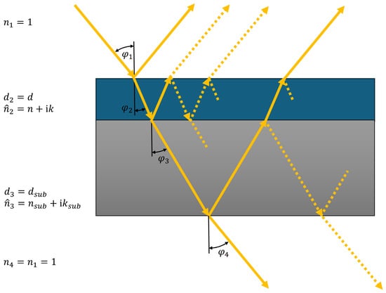
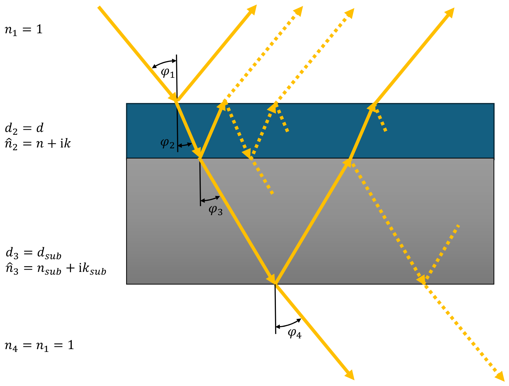
In optical coating design, the optical constants of the corresponding materials are assumed to be known, and only the layer sequence and their thicknesses are determined. The process-specific optical constants are usually determined on suitable single layers using spectrophotometry or/and ellipsometry in terms of a reverse search procedure [6,7,8,9,10]. For dielectric layers in the transparency range, this is a routine task for which different methods have been established depending on the available measurement technology [11,12,13,14,15,16]. The characterization of such a single layer on a known (often transparent) substrate can already be performed in the frames of the model of a homogeneous thin solid film with smooth and parallel interfaces (Figure 1) by means of spectral transmission measurement and the use of a simple dispersion model (e.g., Cauchy or Sellmeier) [17].
Figure 1.
Model of a homogeneous single layer coating (refractive index , extinction coefficient , thickness , coherent light propagation) with smooth and parallel interfaces on a known substrate (refractive index , extinction coefficient , thickness , incoherent light propagation) with air as ambient medium at the front and back sides of the coating. Contributions of different light paths (yellow lines) and relevant angles are indicated. Thicknesses are not true to scale, because is assumed. In absorbing materials, the propagation angles must be tackled as complex parameters.
By incorporating spectral reflectance data, a reliable characterization is also possible in spectral regions where weak absorption occurs. This simple approach fails when the absorption becomes so strong that the transmission signal practically disappears. This is the case for typical high-refractive-index coating materials (TiO2, Ta2O5, Nb2O5, ZrO2, and HfO2) in the ultraviolet spectral range at coating thicknesses that cause significant interference effects in the visible spectral range. Usually, this concerns coatings with an optical thickness of a few hundred nanometers.
A general problem in optical coating characterization is in the ambiguity of the obtained optical constants [18,19], caused by a multiplicity of mathematical solutions of the corresponding reverse search task. Therefore, additional information is required to determine the optical constants (refractive index , extinction coefficient ) unambiguously.
This article focuses on the choice of optical measurements best suited for reducing the ambiguity of the reverse search task when strong absorption occurs. Moreover, a numerical criterion for excluding improper combinations of measurements will be proposed. In contrast to the famous study [20], we will consider films with an optical thickness of the order of the wavelength rather than ultrathin films with thicknesses much smaller than the wavelength. This may be of relevance in the case of material characterization for solar absorber or solar cell applications. Also, the determination of optical constants at the fundamental absorption edge of dielectrics or semiconductors will be addressed this way. This will be illustrated using Nb2O5 and its optical constants published by Franta [21] as a model system.
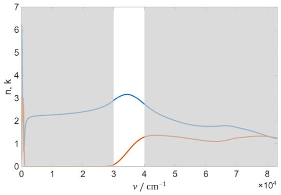
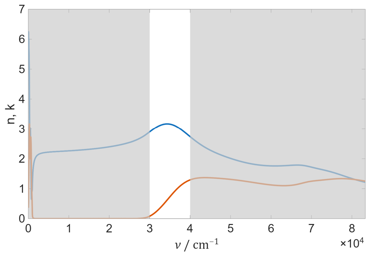
To eliminate non-physical mathematical solutions of the reverse search procedure, the use of a Kramer–Kronig-consistent dispersion model is often favored [21,22]. Note that such models automatically provide access to anomalous dispersion; as evident for Nb2O5, anomalous dispersion can already be observed in the wavelength range up to 250 nm (wavenumber 40,000 cm−1, Figure 2). The wavenumber is related to the vacuum wavelength through .
Figure 2.
Optical constants (blue line) and (orange line) of Nb2O5 [21]; white background indicates spectral range addressed in this article.
The fundamental problem of solution ambiguity already occurs in the strongly idealized film model of homogeneous layers with smooth interfaces (Figure 1). This model is, however, widely used in optical coating practice, and therefore we will perform our study in terms of this model, too. The effect of the implementation of different layer models on the characterization result is exemplified in [23].
Note that the requirement of Kramers–Kronig consistency for eliminating non-physical dispersion solutions will lose efficiency when the investigated spectral range is too narrow. In this case, the elimination of non-physical solutions by a suitable combination of independent measurements may be the method of choice [20,24,25,26,27,28,29,30]. A comparative analysis of the accuracy of reflectance methods for determining the optical constants of highly absorbing films is provided in [31]. The focus of our study is clearly on the elaboration of spectra that lack interference pattern. In this context, the term “narrow spectral range” denotes a spectral range that
- Does not include a relevant interference pattern of the thin-film spectrum;
- Is much too narrow to exhaust typical sum rules [32,33,34].
In the extreme case, that narrow spectral range degenerates to a single wavelength (or wavenumber) value, defining what is called a single-wavelength method [7,23,35]. Frequently, the examples discussed in this study will concern this extreme case.
In Section 2, Section 3, Section 4 and Section 5, we will focus on this situation. Attention will be paid to the choice of angles of incidence. Emphasis will be placed on near-normal incidence as well as incidence angles in the region of the pseudo-Brewster’s angle (which minimizes the surface reflectance at p-polarization [36,37]), as well as the second Brewster’s angle (which minimizes the ratio of surface reflectances at p- and s-polarization [38]). In the case of dielectric coatings at the absorption edge, the difference of both angles is commonly small [39]. Clearly, the knowledge of the pseudo-Brewster angle and corresponding reflectance for p-polarization can be used for a direct determination of the optical constants [40,41,42,43].
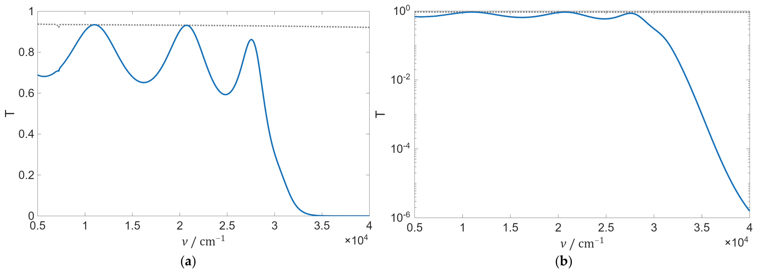
A suitable geometrical layer thickness of a highly refractive single layer for characterization in the UV/VIS/NIR spectral range is around 200 nm. The theoretical transmittance of such a Nb2O5 layer on a 1 mm thick quartz glass substrate is shown in Figure 3a. Several transmittance extrema can be observed in the transparency range, providing access to the optical thickness of the film [19,44]. At the same time, the refractive index can be determined by making use of envelope methods [45]. In the wavenumber range above 35,000 cm−1, the transmission signal disappears almost completely. In fact, however, it is only very small and can still be reliably detected with a standard spectrophotometer. This is clearly visible in the logarithmic representation (Figure 3b). This form of representation is common, as, for example, the optical density is often specified for neutral density filters [46] instead of the transmittance. The following applies to the relationship between the two variables.
The detectable optical density here is 6, which is significantly below the optical density of 8 specified by PerkinElmer for the Lambda 1050+ spectrophotometer [47]. Since this measurement is relatively easy to perform, it provides valuable information for characterization and will be further discussed later. If the available spectrophotometer is unable to detect the required optical density, the inclusion of an additional sample with a smaller layer thickness may be helpful. For a Nb2O5 layer thickness of 50 nm, a significant transmission signal with approx. 0.027 is still available on a quartz glass substrate at 40,000 cm−1. However, it should be noted that deviating layer properties may occur in the growth zone (e.g., in the case of Ta2O5 [48]). In this case, the model of homogeneous, isotropic layers considered here cannot find application.
Figure 3.
Linear (a)- and logarithmic (b)-scaled theoretical transmittance at normal incidence of the uncoated fused silica substrate (dotted line, = 1 mm, optical constants from [49]) and with a Nb2O5 single layer (solid line, = 200 nm, optical constants from [21]).
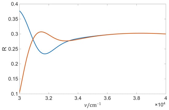
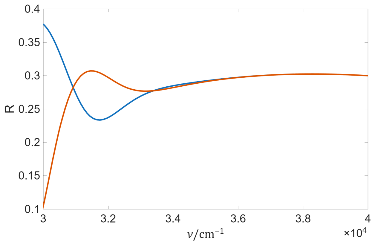
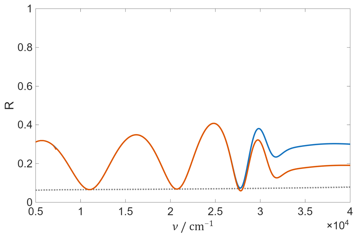
While the use of transmission measurements requires application of a transparent substrate, the choice of the substrate is almost irrelevant for the result of the reflection measurement of absorbing coatings. Accordingly, the reflection spectra for wavenumbers above approx. 35,000 cm−1 of the mentioned Nb2O5 film are practically identical for substrates made of quartz (optical constants from [49]) or silicon (optical constants from [50]), while they differ significantly for smaller wavenumbers (Figure 4).
Figure 4.
Normal incidence theoretical reflectance of a Nb2O5 single layer ( = 200 nm, optical constants from [21]) on a fused silica (blue line, optical constants from [49]) and silicon (orange line, optical constants from [50]) substrate ( = 1 mm).
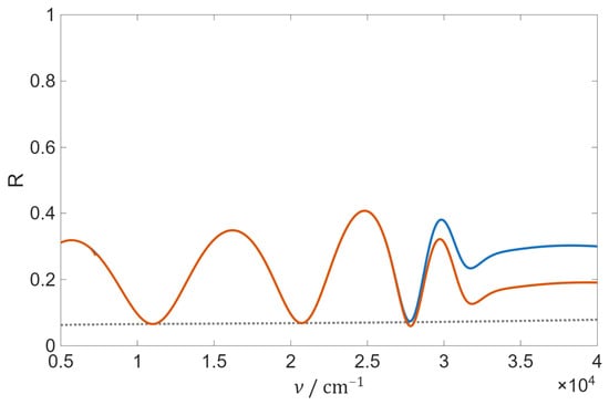
The use of a transparent substrate for characterization in the absorption edge region nevertheless provides access to potentially useful additional information, since the reflections measured from the front and back sides differ in lossy layer systems [51]. For the 200 nm thick Nb2O5 layer on a quartz glass substrate, the front and back side reflectances differ by up to 0.1 (Figure 5).
Figure 5.
Normal incidence reflectance of a Nb2O5 single layer ( = 200 nm, optical constants from [21]) on a fused silica substrate ( = 1 mm, optical constants from [49]) from the front (orange line) and back sides (blue line). Dotted line indicates the normal incidence reflectance of the uncoated substrate.
For characterization using ellipsometry, measurements are usually taken in reflection at large angles of incidence. The classical ellipsometric angles and are derived from the ratio of the complex reflection coefficients and for s- and p-polarization, respectively.
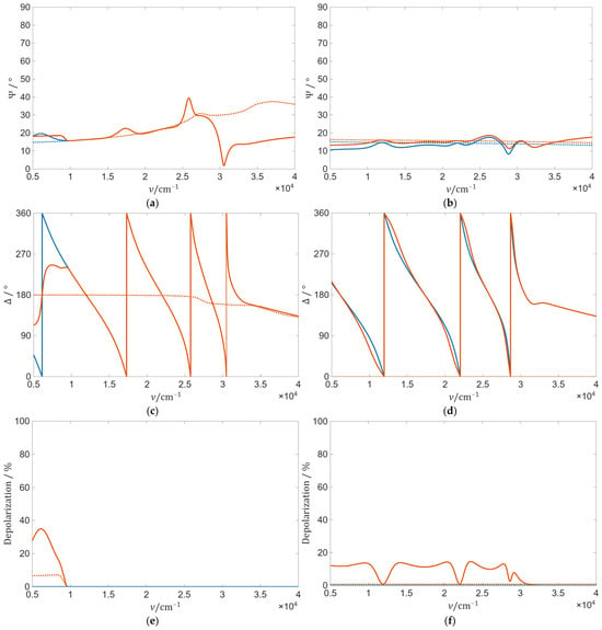
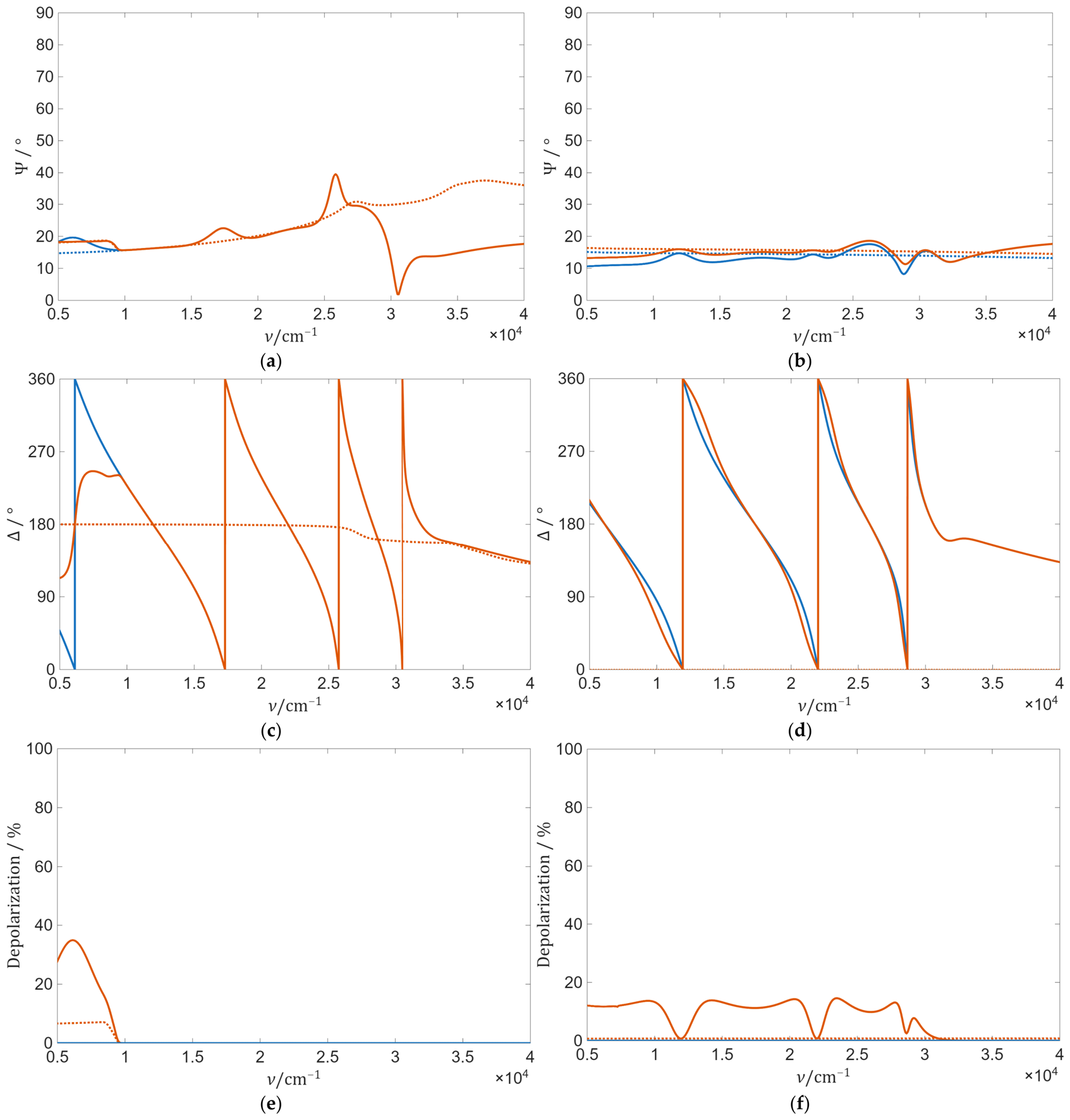
In the thin-film system shown in Figure 1, an interface between the substrate and air (the substrate back side) is included, which is often neglected in ellipsometry. Instead, a semi-infinite substrate is assumed. Reflections from this interface cause a modification of the measurement signal and result in depolarization. Equation (2) is strictly valid only for non-depolarizing systems. Otherwise, the Stokes–Mueller formalism must be applied [52]. Therefore, three independent normalized Mueller matrix elements are used. They can be converted to the classical ellipsometric angles [53], but the introduction of a depolarization factor as a third parameter is required. Clearly, this effect disappears when the layer or the substrate is intransparent. Figure 6 shows the ellipsometric angles and the degree of depolarization for a 200 nm thick Nb2O5 single layer on both quartz and silicon substrates, with and without consideration of the substrate back side. In Figure 6a,c, the impact of the depolarization on the ellipsometric angles could be neglected for wavenumbers above the absorption edge of silicon (~10,000 cm−1). On the fused silica substrate, the transmittance of the layer must be sufficiently small (valid above appr. 30,000 cm−1) to suppress this impact. This could be directly seen in the depolarization (Figure 6e,f). Clearly, in the case of classical ellipsometry, the depolarization is always zero.
Figure 6.
Ellipsometric angles (a,b), (c,d) and depolarization (e,f) at 65° angle of incidence for a Nb2O5 single layer ( = 200 nm, optical constants from [21]) with (orange line, = 1 mm) and without (blue) consideration of the substrate back side (silicon with optical constants from [50] in (a,c,e) and fused silica with optical constants from [49] in (b,d,f)). Dotted lines indicate normal incidence reflectance of the uncoated substrate.
2. Theoretical Aspects
Front side reflectance , back side reflectance , and transmittance of the film system shown in Figure 1 can be calculated in terms of the following couple of equations:
with
and
The polarization dependence (s- or p-polarization) is hidden in Fresnel’s formulas (here written in the Mueller convention [54]):
The theoretical spectra shown in Figure 3, Figure 4 and Figure 5 have been calculated in terms of these equations.
If the film (material 2 in Figure 1) absorption is sufficiently strong (), simpler equations (compare Appendix A) may find application. Then, the front side reflectance may be approximated by a single interface between a transparent medium with refractive index and an absorbing medium with refractive index and extinction coefficient , where the complex refractive index is given by the relationship .
Let us now turn to a graphical representation in terms of the contours of constant reflectance in the - plane (compare [20]). We will call them iso-reflectance curves. Since both the normal incidence iso-reflectance curves for front and back side reflectances of strongly absorbing films on a thick substrate can be represented as circles in the - plane (compare Appendix A), in this study, this form of representation is used. Other representations that use the real and imaginary parts of the dielectric function instead can be found in the literature, for example for contour lines of the pseudo-Brewster angle [36]. Similar contour plots can also be found for other quantities [55,56,57].
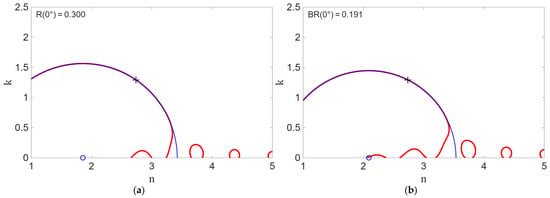
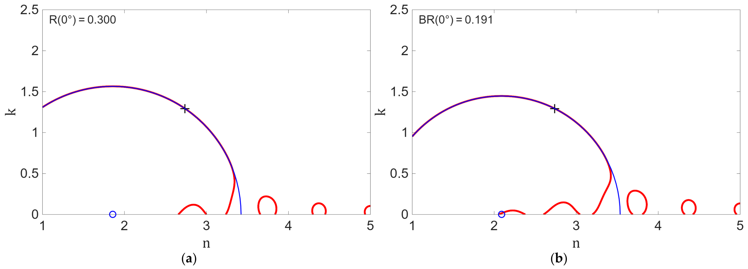
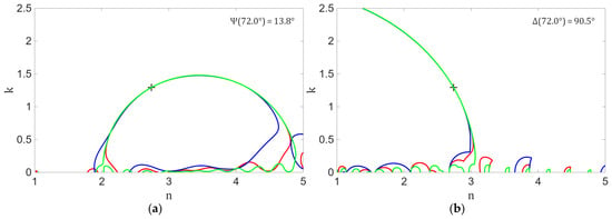
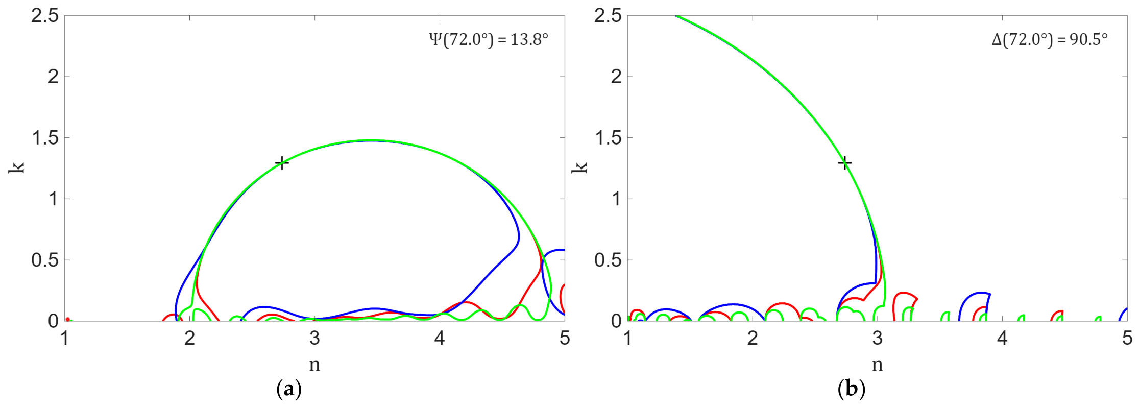
Figure 7 exemplifies iso-reflectance curves for the and using the thin-film model from Figure 1 (Equations (3)–(6) assuming normal incidence) as red lines. The calculations are performed for a 200 nm thick Nb2O5 layer (optical constants from [21] are indicated by a black cross) on a 1 mm thick quartz glass substrate (optical constants from [49]) with air as the ambient medium for a wavenumber of 40,000 cm−1 (wavelength 250 nm). The shape of the iso-reflectance curves according to (3)–(6) is much more complex than the simple circles described by Equations (A2) and (A6) (large blue circle with the center indicated by a small circle) in Appendix A. In the range of low extinction coefficients, there are several additional contours that correspond to different refractive indices. This multiplicity of possible - pairs is a consequence of interference in the single layer coating and therefore only occurs when the extinction coefficient is sufficiently small [58]. In spectroscopy practice, they define a set of multiple solutions of the reverse task, when and are to be calculated from a measured reflectance. These potential but physically non-valid solutions can be ruled out by means of an additional transmission measurement. At larger extinction coefficients, the red iso-reflectance curve practically coincides with the circle predicted by Equation (A2) or (A6) (blue curve).
Figure 7.
Iso-reflectance at 40,000 cm−1 for (a) and (b) at normal incidence (red lines) for a Nb2O5 single layer ( = 200 nm, optical constants from [21] are indicated by a black cross) on the fused silica substrate ( = 1 mm, optical constants from [49]); blue lines: circles according to Equations (A2) and (A6) with indicated center positions.
At oblique incidence, the expressions for the polarization-dependent photometric and ellipsometry quantities become more complex, and analytical expressions for the corresponding “iso-observable” plots become unwieldy, if they can be derived at all.
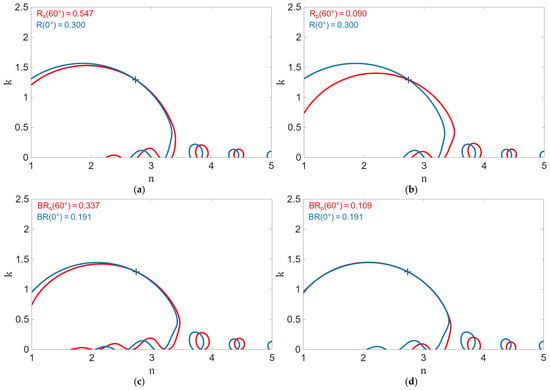
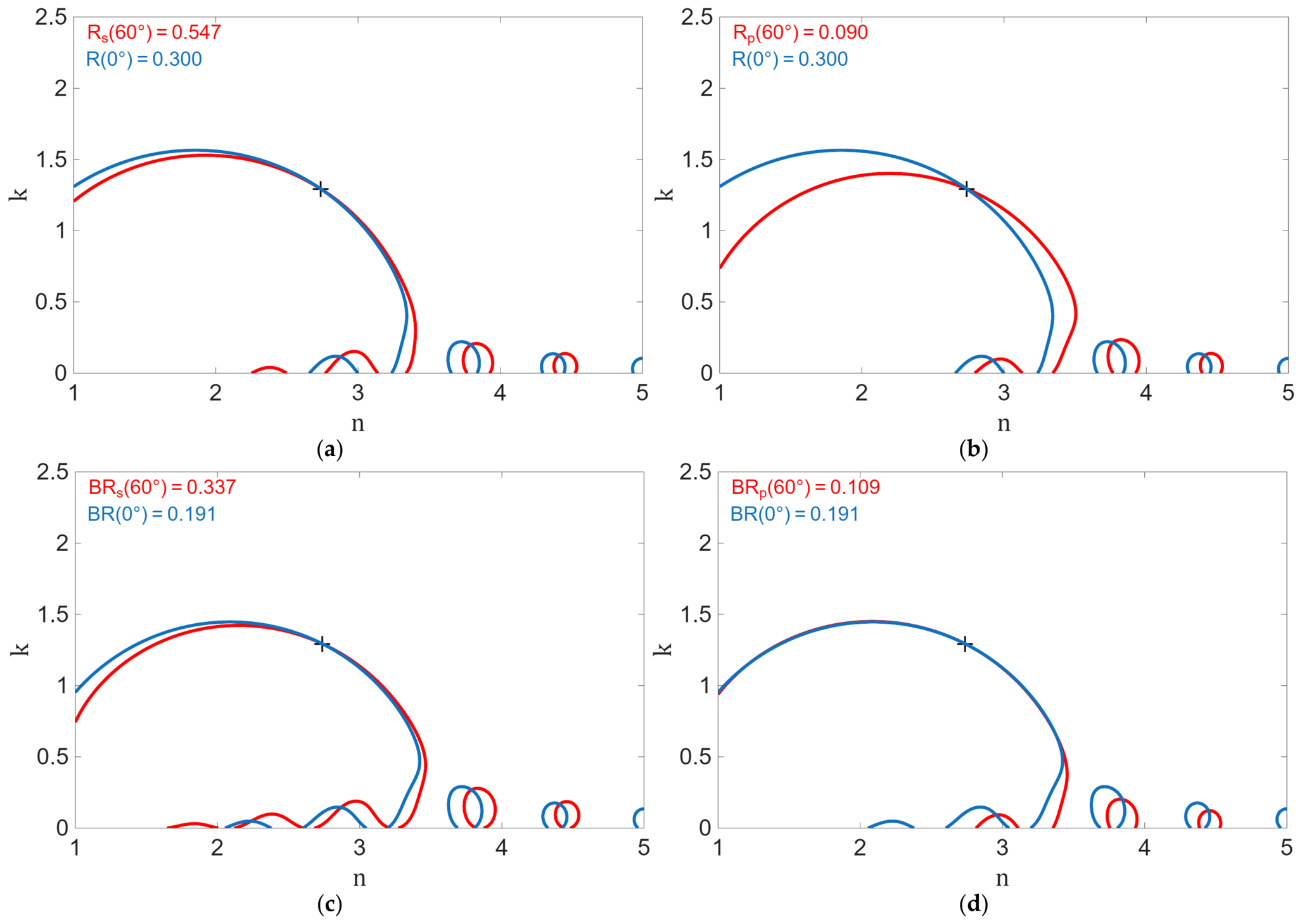
Regardless of the availability of analytical expressions, such iso-reflectance or “iso-observable” plots are useful for identifying useful combinations for the unambiguous determination of and from corresponding spectral data. Clearly, from the single normal incidence reflectance at 40,000 cm−1, according to Figure 7, and cannot be determined unambiguously. The inclusion of a second measurement would add a further “iso-observable” curve that should result in an intersection with the curves from Figure 7 at the correct pair of and [20]. This is exemplified in Figure 8. Here, in addition to the iso-reflectance curves according to Equation (A2) (Figure 8a,b) and Equation (A6) (Figure 8c,d), iso-reflectance curves according to (3)–(6) for an incidence angle of 60° are shown.
Figure 8.
Iso-reflectance at 40,000 cm−1 for (a,b) and (c,d) for 60° angle of incidence (red line) and normal incidence (blue line) for a Nb2O5 single layer ( = 200 nm, optical constants from [21] are indicated by a black cross) on the fused silica substrate ( = 1 mm, optical constants from [49]).
Note that in Figure 8, regardless of the chosen combination of measurements, there are a certain number of intersection points of the blue and red curves, still defining a set of multiple solutions of the corresponding reverse search task. In Figure 8, the correct solution is again highlighted by a cross. In real characterization practice, however, mathematically correct but physically senseless solutions need to be eliminated to select the physically meaningful solution. As seen from Figure 8, it is a proper choice of measurement that is crucial for the identification of the correct solution. In fact, a reliable identification of the correct and pair can only be expected in the situation highlighted in Figure 8b, corresponding to a combination of normal incidence front side reflection with front side reflection at 60° at p-polarization. In this situation, although a few discrete intersection points between the blue and red curves exist, the “solutions” corresponding to a small extinction can easily be excluded by an additional transmission measurement. This way, the solution marked with the cross may be certainly identified. In other situations, in addition to the intersection points at low extinction, the iso-reflectance curves at normal and oblique incidence are practically coinciding at larger , providing no chance for the identification of the correct solution.
3. Simulation Results
3.1. Ellipsometry and Photometric Quantities
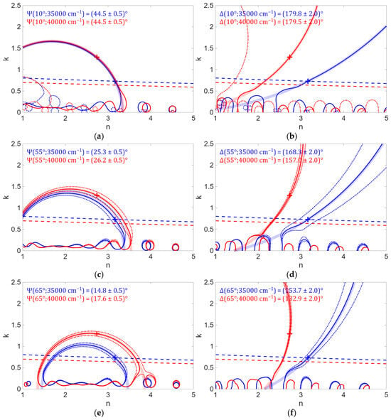
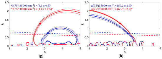
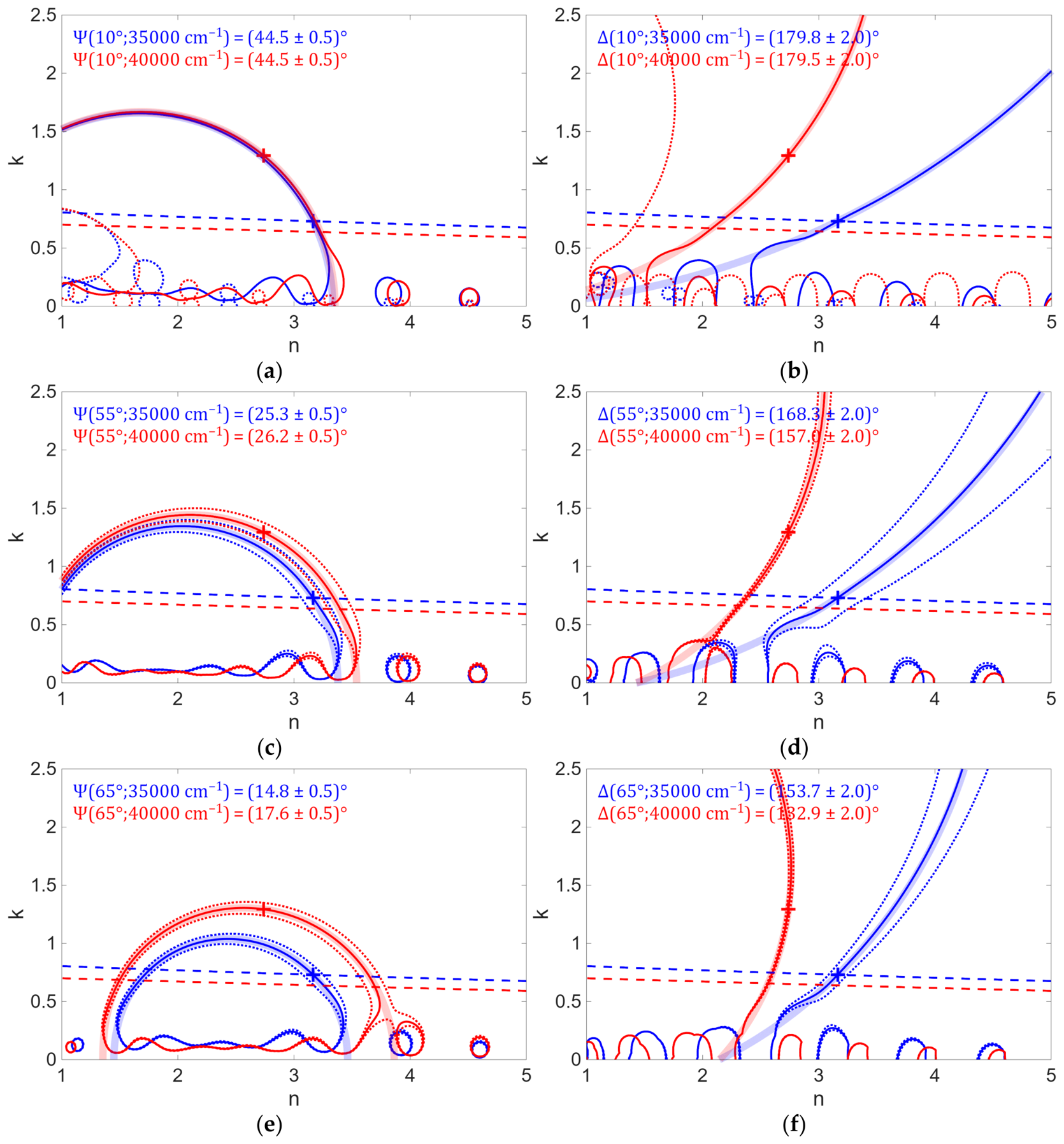
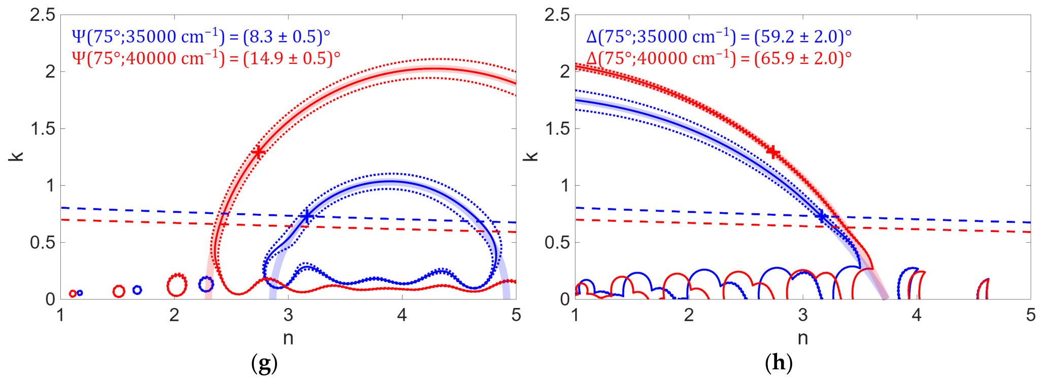
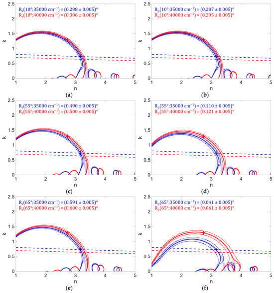
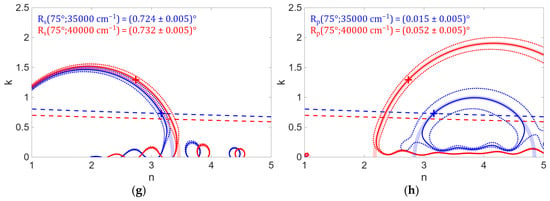
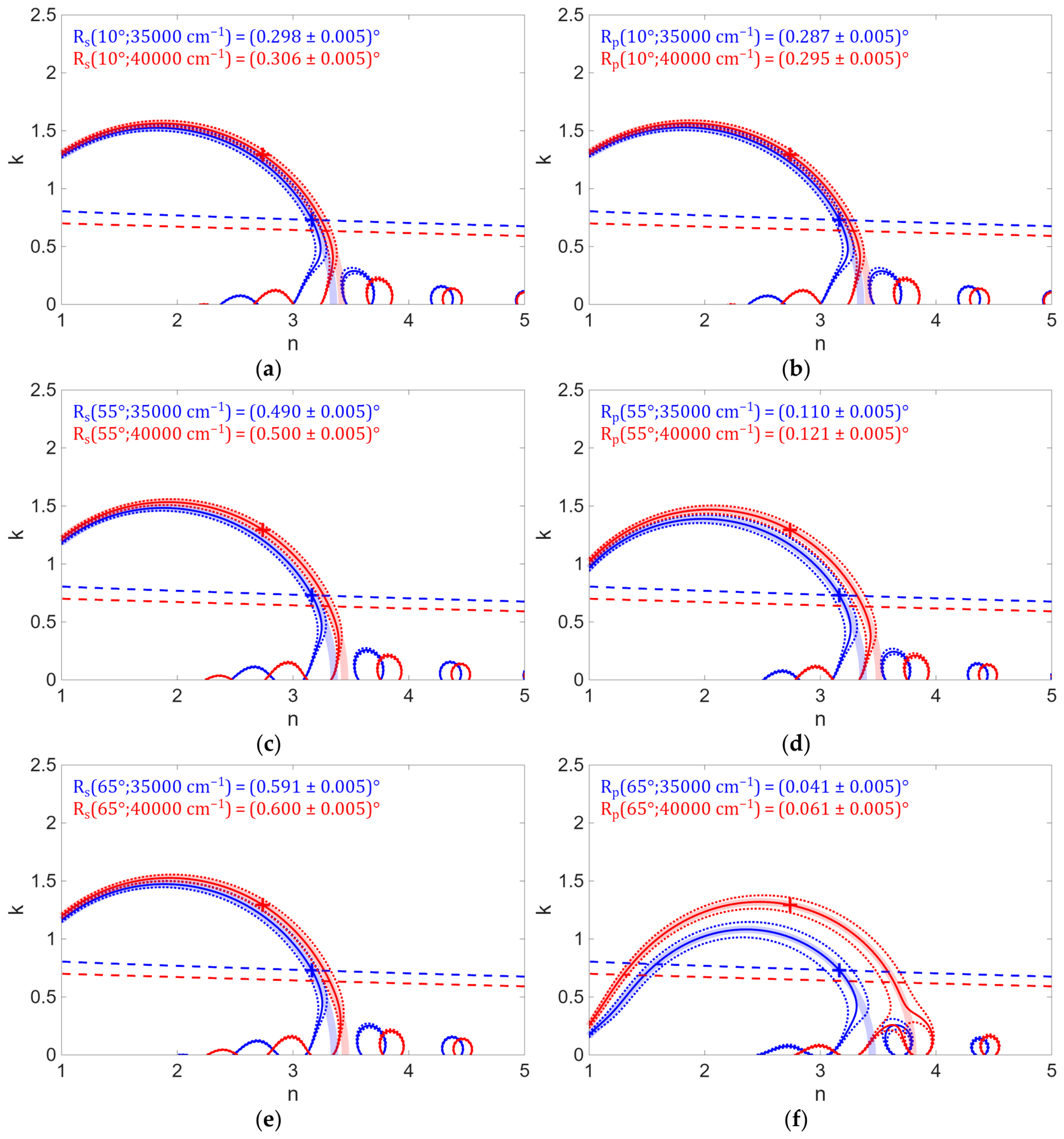
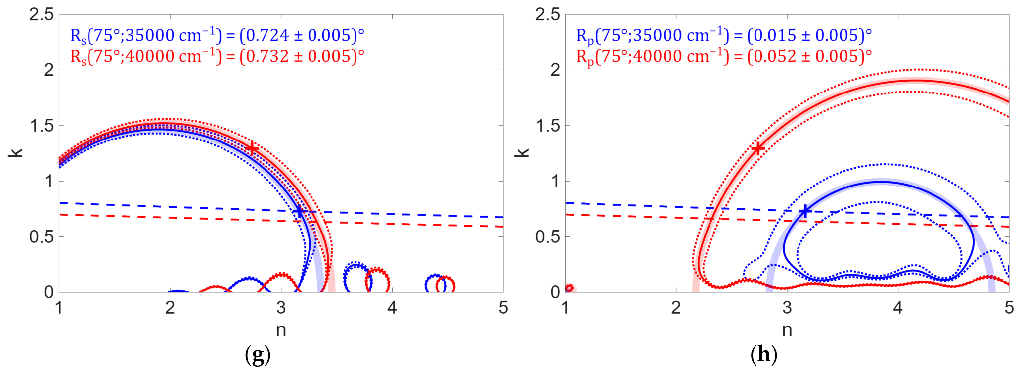
This section presents “iso-observable” plots of the ellipsometry parameters (Figure 9) and the reflectance for s- and p-polarized light (Figure 10) for nearly perpendicular light incidence (10° angle of incidence) and large angles of incidence (55°, 65°, and 75°) for the single layer coating according to Figure 1. The selected range of large angles of incidence is common for ellipsometry and can also be covered by photometry [59,60,61,62]. The behavior at the onset of the absorption edge (35,000 cm−1) is shown in blue. Here, the transmittance drops below 0.001 (, and interference effects lose significance (Figure 3). Additionally, the impact of the substrate on the reflected signals can be neglected (Figure 4), and the ellipsometric angles are not affected by depolarization (Figure 6). On the other hand, typical commercial polarizers are specified for wavenumbers below 40,000 cm−1 only, while a wavenumber of 40,000 cm−1 corresponds to an for a 200 nm Nb2O5 layer. Despite the already mentioned reference wavenumber of 35,000 cm−1, the wavenumber of 40,000 cm−1 was therefore selected as the second reference wavenumber; the corresponding dependencies are shown in red. The underlying optical constants of Nb2O5 are represented by crosses colored accordingly. Numerical values of the optical constants at these wavenumbers and assumed thicknesses for the single layer coating according to Figure 1 are summarized in Table 1.
Figure 9.
“Iso-observables” (solid lines) for ellipsometric values (left) and (right) of a single layer coating according to Table 1 at different angles of incidence: (a) at 10°; (b) at 10°; (c) at 55°; (d) at 55°; (e) at 65°; (f) at 65°; (g) at 75°; (h) at 75°) for the reference wavenumbers (blue: 35,000 cm−1, red: 40,000 cm−1). Error sensitivity for and (dotted lines), iso-transmittance for at normal incidence (dashed lines), corresponding “iso-observables” of a Nb2O5-air-interface (thick, semi-transparent lines), and optical constants of the layer (cross) are additionally indicated.
Figure 10.
Iso-reflectance’s (solid lines) for (left) and (right) of a single layer coating according to Table 1 at different angles of incidence: (a) at 10°; (b) at 10°; (c) at 55°; (d) at 55°; (e) at 65°; (f) at 65°; (g) at 75°; (h) at 75°) for the reference wavenumbers (blue: 35,000 cm−1, red: 40,000 cm−1). Error sensitivity for (dotted lines), iso-transmittance for at normal incidence (dashed lines), corresponding iso-reflectance’s of a Nb2O5-air-interface (thick, semi-transparent lines), and optical constants of the layer (cross) are additionally indicated.
Table 1.
Optical constants and thicknesses for the single layer coating according to Figure 1.
The solid lines correspond to the “iso-observable” plots for the exact theoretical value of the respective observable, calculated in terms of Equations (3)–(6). The dotted lines provide information about the error sensitivity. They indicate deviations in optical constants, when tolerances in the measured quantities are assumed. In the graphs, an uncertainty of 0.5° was assumed for and an uncertainty of 2° for . Thus, the relative uncertainties related to the possible range of values are the same for both quantities. Clearly, these uncertainties are larger than reported values [63], but more illustrative for the graphical representation. A measurement uncertainty of 0.005 was assumed for the reflectance for both polarizations. Furthermore, iso-transmittance curves corresponding to T= 0.001 are indicated as dashed lines. The respective plots for the discussed simplified model of an infinitely thick Nb2O5 layer—i.e., a single interface in measurements from the front side—are represented by thick, semi-transparent lines in the respective color.
Qualitatively, the graphs shown look different from those published in [20]. When comparing with [20], it should be taken into account that [20] addresses the characterization of thin metals films, with thicknesses considerably smaller than the wavelength. Our study is on the analysis of semiconductor films near the absorption edge, with optical thicknesses on the order of the wavelength, which is the basic difference from the systems discussed in [20].
3.2. Merged Discrepancy Functions
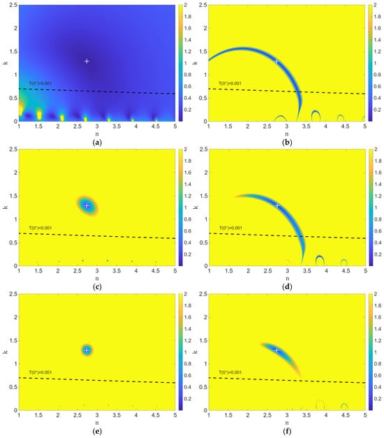
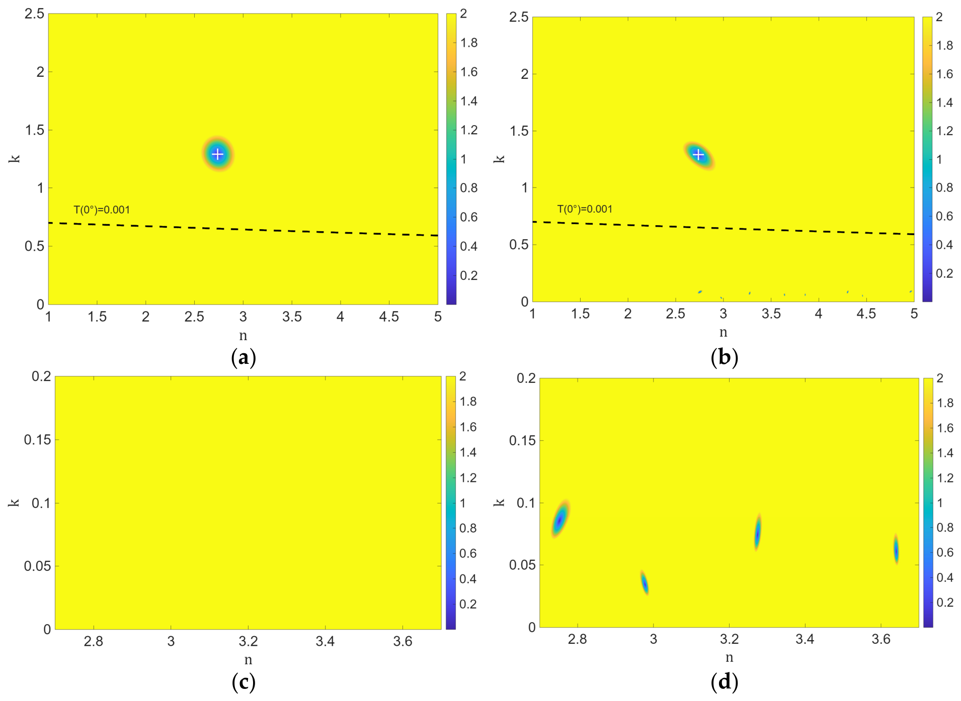
Figure 11 shows the discrepancy function () for the ellipsometry parameters and for the reflectances and at the specified angles of incidence. For , the widely used average root mean square deviation is used [7]. Therefore, a number of observables can be considered, while the deviation from the corresponding target value is weighted according to the tolerance :
Figure 11.
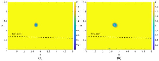
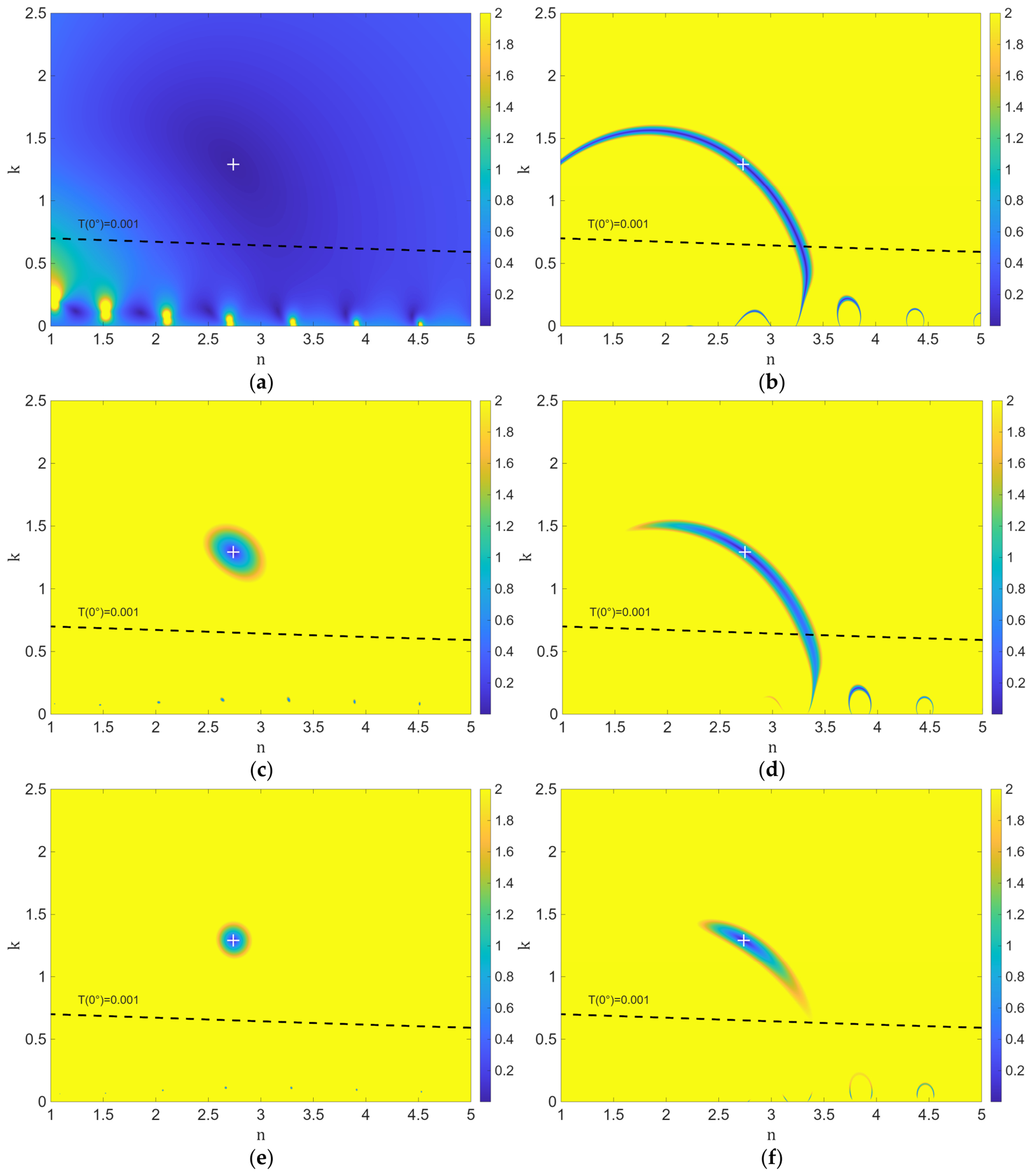
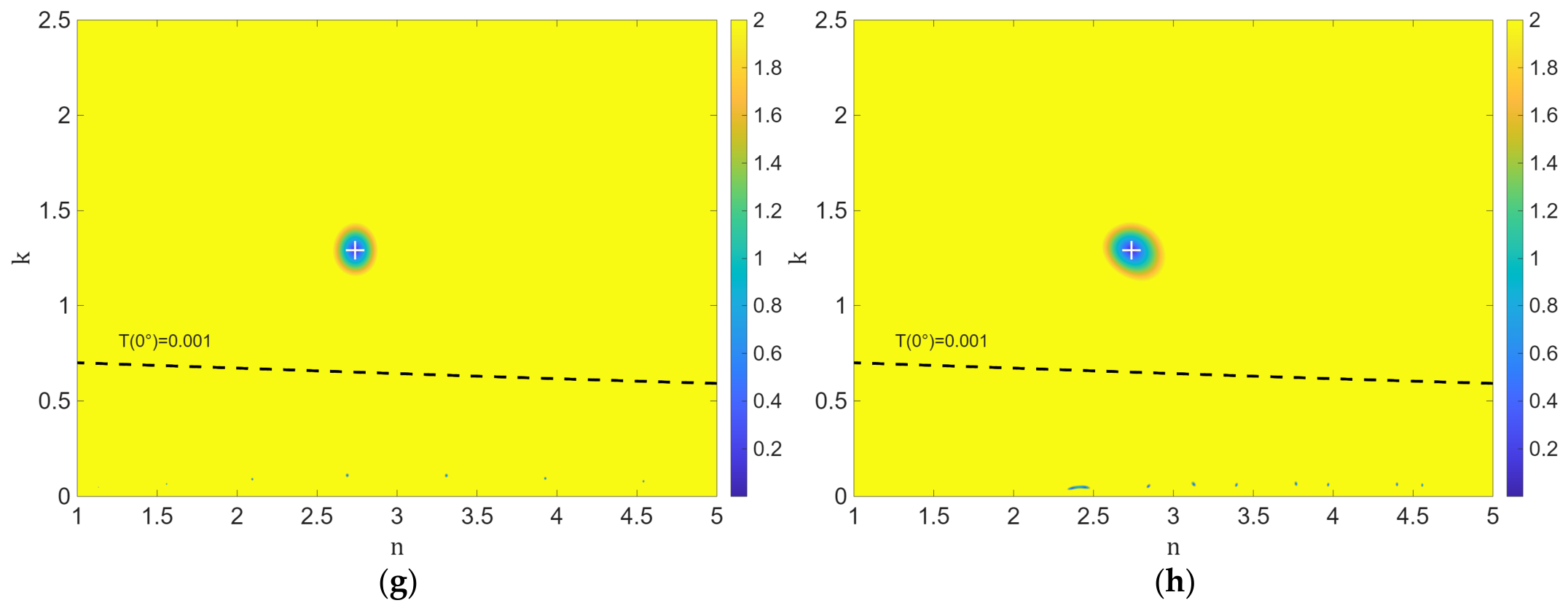
Combined at 40,000 cm−1 (according to the color code defined on the right ordinate) of a single layer coating according to Table 1 for ellipsometric angles ((left): , , , ) and polarization-dependent reflectance ((right): , , , ) at different angles of incidence. (a) combined for ellipsometric angles at 10°; (b) combined for polarization-dependent reflectance at 10°; (c) combined for ellipsometric angles at 55°; (d) for polarization-dependent reflectance at 55°; (e) combined for ellipsometric angles at 65°; (f) for polarization-dependent reflectance at 65°; (g) combined for ellipsometric angles at 75°; (h) for polarization-dependent reflectance at 75°). Optical constants of the layer are indicated by a white cross and iso-transmittance for T = 0.001 at normal incidence by a black dashed line.
In this description, mathematical solutions of the reverse search (finding and from measured data) are represented by local minima in the . When light is incident nearly perpendicularly, the impact of polarization is small, and ellipsometry parameters naturally do not make a significant contribution to finding the correct solution, although the “iso-observable” plots of and intersect nearly orthogonally (Figure 9). The reason is that the corresponding local minimum (Figure 11a) is very shallow, thus reducing the efficiency of local minimum search algorithms. In combination with other measurements performed at different angles of incidence, they may be helpful for eliminating unphysical multiple solutions observed in the small extinction region. This has a rather transparent physical background. Multiple minima of the may be caused by interference effects, the latter being strongly dependent on the incidence angle. However, a transmission measurement is clearly superior for ruling out incorrect solutions, since all local minima with k < 0.5 can be excluded with a transmission threshold of 0.001 (black dashed line).
The local minimum remaining in the ellipsometry parameters coincides with the global minimum in the discussed range of optical constants and, at large angles of incidence, is well-defined by an elliptical region (Figure 11c,e,g). This is advantageous for local optimization methods. The situation is different for the reflectance (Figure 11b,d,e). Here, the contours are more crescent-shaped, and many nearly equivalent minima of correspond to significantly different optical constants. Only at large angles of incidence does the valley in the come close to an elliptic shape (Figure 11h).
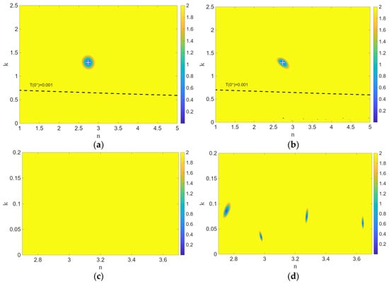
When multiple angles of incidence are combined (Figure 12a), combining the angles of incidence 55°, 65° and 75° results in only a slight improvement in the ellipsometry parameters (on the left), but eliminates local minima in the region of low extinction coefficients (Figure 12c).
Figure 12.
Combined at 40,000 cm−1 (according to the color code defined on the right ordinate) of a single layer coating according to Table 1 for ellipsometric angles and at 55°, 65° and 75° (left) and for at 10° and 75° (right). (a) combined for ellipsometric angles; (b) combined for ; (c) Magnified plot of (a); (d) Magnified plot of (b). Tolerances are identical to the similar values used in Figure 10 and Figure 11. Optical constants of the layer are indicated by a white cross and iso-transmittance for T = 0.001 at normal incidence by a black dashed line. Magnified plots (bottom) are provided for a region of low extinction coefficients, which potentially contains multiple local minima.
Similarly, a single reflectance measurement at a small incidence angle, combined with a reflectance measurement at an angle of incidence of 75° and p-polarization, can effectively narrow the range of possible solutions (Figure 12b). Here, we have numerous local minima in the region of low extinction coefficients (Figure 12b,d), which can be most efficiently eliminated by performing a transmission measurement with normal light incidence.
4. Discussion
4.1. Numerical Criterion for Measurement Choice
The “iso-observable” curves presented in Section 3.1 provide some guidance for a proper selection of combinations of ellipsometry and photometric quantities for a reliable characterization of single layer coatings at the absorption edge. The application of a combined (Section 3.2) already demonstrates that the combination of ellipsometry quantities at angle of incidence above 55° results in a well-defined, elliptically shaped local minimum at the correct solution. In the case of polarization-dependent reflectance, this could only be observed for 75° angle of incidence, in agreement with what has been found in [20,31] for thin metal films. Otherwise, a large, crescent-shaped area is observed, which cannot sufficiently narrow the range of mathematical solutions.
Clearly, the combination of many different measurements can solve this problem [21,64,65,66,67,68] and is essential when more complicated coating models (including multilayer coatings [69,70,71], inhomogeneities [72,73,74,75], anisotropy [76,77], interface roughness [78], photochromic [79] and photoluminescence coatings [80]) are considered. However, in characterization practice, the number of available measurements may be limited by both available measurement time and equipment. When restricted to a combination of two measurements, an identification of the intersection point of the corresponding iso-observable curves will be strongly facilitated when the curves intersect perpendicularly. For two observables and , this requirement may be quantified in terms of the following condition:
where represents the correct - pair (usually indicated by a cross in the graphs).
The following tables summarize calculated values for different choices of the observables in application to the selected Nb2O5 model system. Note that a proper selection of observables (reasonable accuracy in and determination) should result in a rather small value of . On the contrary, when becomes large, is still determined with good accuracy, while the error in is expected to be very large. The opposite case, namely an accurate determination of with a large error in , corresponds to a value close to 1.
In Table 2 is shown for combinations of ellipsometry quantities and . In general, combinations of and at the same angle of incidence result in a vanishing and thus represent a very good choice of measurements (green cells). This is nothing new, but it confirms the validity of the criterion from Equation (8). Additionally, the combination of and for 10° and 75° also provides a small value of . However, the combination of an ellipsometry parameter recorded at φB2 with a parameter recorded at a different angle did not yield any systematic improvement in the parameter . Only the combination of both quantities recorded at the second Brewster’s angle is useful, because of the obvious orthogonality of the iso-observable plots near the crosses (compare Figure 13). This remains essentially true even if the layer thickness is different, provided it is sufficiently large in comparison to the penetration depth of the light.
Table 2.
Numerical values at 40,000 cm−1 of according to Equation (8) for pairs of ellipsometric angles and as observables for the single layer coating according to Table 1. The highlighted combination are a suitable choice for determination of and (green), only (red) and only (yellow).
Figure 13.
Iso--plots (a) and Iso--plots (b) at the second Brewster angle for a single layer coating according to Figure 1 at 40,000 cm−1 for different layer thicknesses: 100 nm (blue), 200 nm (red) and 400 nm (green). Optical constants of the single layer coating are indicated by a black cross.
Additionally, some combinations appear to be a good choice for either (red cell) or (yellow cell) determination. Thus becomes large when is recorded at an angle of incidence close to second Brewster angle [38] (here 72.0°). At this angle, has a minimum, which has direct consequences on the behavior of the ellipsometry parameters (compare (2)). Contrarily, the combination of Ψ values recorded at 55° and 65° results in a closest to one, indicating highest accuracy in determination.
In the case of combining and , we get quite different results for the impact of the angle of incidence (Table 3). Now, the variations in are rather small. Very large values () are not observed, and values for the best choices are still larger than zero. For good accuracy, the inclusion of at 75° angle of incidence is obviously essential (green fields in Table 3), again in agreement with the situation reported for thin metal films [20,31]. When looking at Figure 10, this becomes instantly clear, because only at a 75° angle of incidence shows a significantly different shape in the iso-reflectance plot compared to the corresponding shapes at other angles of incidence. This is clearly related to the key role of the pseudo-Brewster angle [36,37] (here 71.4°). According to Equation (A3), the center position of the circle depends on the ratio and has its minimum at the pseudo-Brewster angle for p-polarization.
Table 3.
Numerical values at 40,000 cm−1 of according to Equation (8) for pairs of and as observables for the single layer coating according to Table 1. The green highlighted combinations are a suitable choice for determination of and .
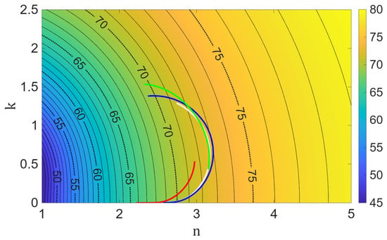
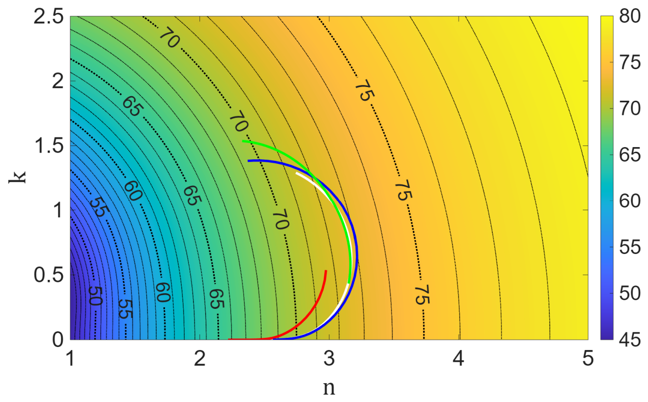
The importance of at 75° also persists for other relevant high-refractive-index materials. Iso- plots (Figure 14, dotted lines) clearly show that this quantity varies only marginally (~70°…73°) in the vicinity of the absorption edge (Figure 14, solid lines).
Figure 14.
Iso- plot (dotted black lines) and optical constants of Nb2O5 [21] (white solid line), Ta2O5 [48] (red solid line), TiO2 [81] (blue solid line) and ZrO2 [82] (green solid line) in the spectral range 25,000 cm−1–40,000 cm−1.
Among the angles investigated in Table 3, it is only the angle of incidence of 75° that exceeds the pseudo-Brewster angle.
Note that, according to Table 3, the combinations of observables favored in Figure 11 ( and at 75°) as well as in Figure 12 ( at 10° and 75°) clearly belong to the combinations favored in terms of Equation (8).
When combining ellipsometry values and polarization-dependent reflectance (Table 4), the best combination is provided by and if both are recorded at 55° angle of incidence. From a practical point of view, these kinds of combinations are not a good choice because commonly and are measured together and should be therefore both used for characterization. For this reason, a generalized approach for at least three quantities should be applied instead. Note, in this context, that the discussion of iso-observable plots may easily be extended to more than two observables.
Table 4.
Numerical values at 40,000 cm−1 of according to Equation (8) for mixed pairs of observables for the single layer coating according to Table 1. The highlighted combination are a suitable choice for determination of and (green), only (red) and only (yellow).
4.2. Physical Interpretation
We now turn to a discussion of the results highlighted in Section 4.1. First of all, let us note that, in s-polarization, the electric field strength vector in the incident light wave is always tangential to the interface, regardless of the incidence angle. Therefore, the electric field strength is always continuous at the interface, and combining reflectance measurements in s-polarization at different angles of incidence is not expected to provide additional information. This is consistent with Table 3, where neither of the combinations provides prominent values.
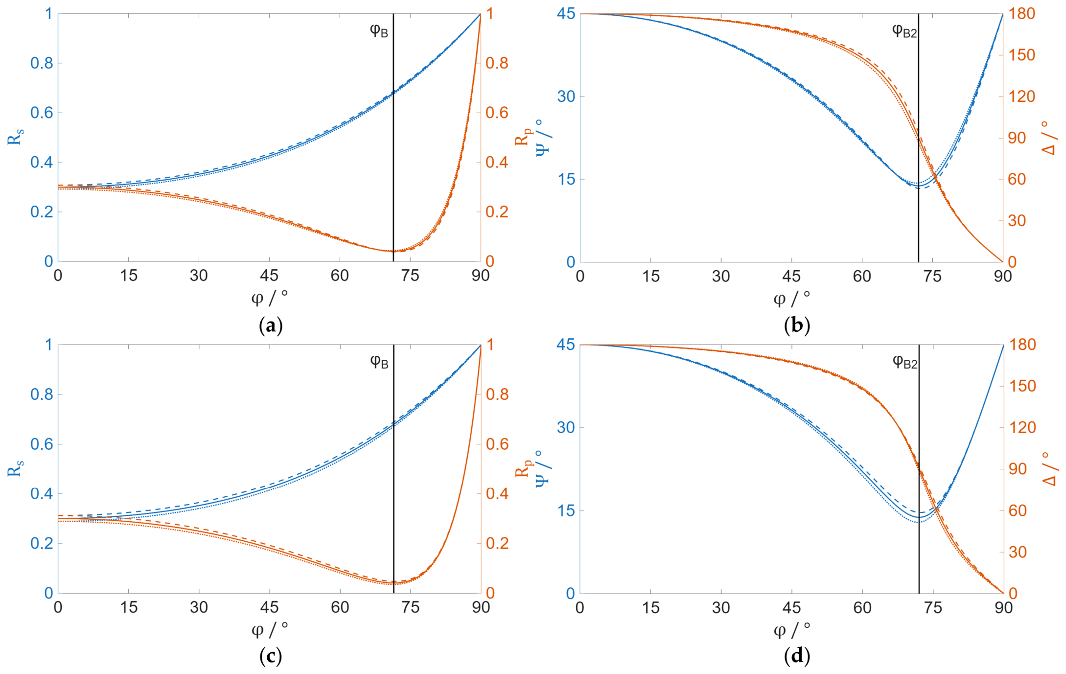
Figure 15 provides calculations of angular scans for , , and at an interface between air and Nb2O5, assuming the optical constants from Table 1 at 40,000 cm−1. The angular scans of do not show any prominent features when or is changed.
Figure 15.
Angular scans for (blue, left axes) and (orange, right axes) in (a,c); (blue, left axes) and (orange, right axes) in (b,d) for an interface of an absorbing material to air. (a) and for 1.293 † and different : 2.638 (dashed), 2.738 † (solid) and 2.838 (dotted). (b) and for 1.293 † and different : 2.638 (dashed), 2.738 † (solid) and 2.838 (dotted). (c) and for 2.738 † and different : 1.193 (dashed), 1.293 † (solid) and 1.393 (dotted). (d) and for 2.738 † and different : 1.193 (dashed), 1.293 † (solid) and 1.393 (dotted). † data for Nb2O5 at 40,000 cm−1 according to Table 1.
The situation is different for . Depending on the angle of incidence, the electric field strength in the incident wave may be decomposed into a tangential (continuous at the interface) and vertical (discontinuous at the interface) contribution. A change in the incident angle changes the relative weight of these contributions, such that combining different angles of incidence provides additional information on the optical constants of the media.
When now looking at Equation (8), we recognize that →0 corresponds to
Hence one of the partial derivatives in Equation (9) must necessarily differ in sign from the other three; otherwise Equation (8) cannot be fulfilled. We now see from Figure 15 that, close to , the sign of does change. Similarly, close to , the signs in and are changing. This provides a vehicle for understanding the role of and in optical characterization, because it might be favorable to combine measurements recorded at angles smaller than the corresponding pseudo-Brewster’s angle with measurements recorded at an angle exceeding the corresponding pseudo-Brewster’s angle. Table 5 summarizes the signs of the corresponding derivatives for prominent green-marked fields in the tables from Section 4.1:
Table 5.
Analysis of favored measurement combinations.
Obviously, criterion Equation (8) is consistent with the signs in the corresponding derivatives as they follow from Figure 15.
Note that at 65°, according to Figure 15d, is insensitive to . This favors rather large values of (see Table 2), corresponding to a bad accuracy in . Contrarily, at 65°, appears to be insensitive to (Figure 15b). Correspondingly, comes close to 1 (compare Table 2 and Table 4).
Hence, criterion Equation (8) appears to be useful for identifying possible combinations of measurements for the reliable determination of and from absorbing thin solid films. The essence of the idea behind Equation (8) is to guarantee a rather symmetrical shape of the minimum of the (Equation (7)). Note that Equation (8) does not provide information on the steepness of the minimum. This is evident from Table 2, where the combination of ellipsometry parameters at 10° clearly minimizes Equation (8), although it is clear from the top left of Figure 11 that the minimum, although symmetric, is too shallow for reliable - determination. An exclusion of shallow minima indeed requires a detailed discussion of the , for example a numerical mapping, as exemplified in Section 2. Alternatively, information on the curvature radii of the DF nearby a local minimum might be included into (8), making use of the second derivatives of the observables. Qualitative physical discussions of the impact of different polarization directions in the given illumination geometry may be helpful, too.
In the version discussed in the present study, Equation (8) therefore has to be regarded as a necessary condition for a proper choice of measurements, but it is not sufficient. After having got a first characterization result from an arbitrarily chosen measurement, Equation (8) may be useful in practice for excluding measurements that are improper for enhancing the accuracy in a refined - determination procedure.
5. Conclusions
In this study, we addressed the choice of measurements applicable for unambiguous determination of the optical constants and of a strongly absorbing thin solid film in a rather limited spectral range. We explicitly addressed the case when the optical film thickness is comparable to or even larger than the wavelength of the incident light. Because of the very small transmittance even in the case of a transparent substrate, emphasis was placed on combining ellipsometry with reflectance measurements at different angles of incidence. Clearly, the choice of the substrate has only a minor impact on these signals when determining optical constants in the absorption edge, and the findings are also relevant for alternative substrates. In order to reduce measurement time and effort, the focus was on the combination of two measurements, although a generalization of the applied strategy to more than two measurements is possible.
Similarly to what has been reported earlier for ultrathin metal films [20], the method of iso-observable plots in the - plane provides an illustrative insight into the arrangement of multiple solutions of the - determination in a practical characterization task. For the particular case of two measurements, we provided a necessary (not sufficient) criterion for the choice of measurements favored for an unambiguous - determination. The criterion makes use of the parameter as defined in Equation (8) and is related to the shape of the minimum in in the - plane as summarized in Table 6:
Table 6.
Important values of .
Depending on the required information, different , and correspondingly different combinations of measurements, may be favored.
Practical simulations concerned the model system of a 200 nm thick Nb2O5 film in the region of the fundamental absorption edge. The simulations reproduced the well-known result that ellipsometry provides a reliable tool for and determination of thin solid films (green fields in the diagonal of Table 2). Nevertheless, alternative suitable combinations of measurements could be identified, too. Among them we note the combination of near-normal incidence reflectance with the reflectance of p-polarized light at a 75° incidence angle. We also have to state that from the simulations performed in this study (Table 1, Table 2 and Table 3), no simple rule of thumb for a proper combination of observables and incidence angles could be identified. It is our point of view that this enhances the value of the criterion from Equation (8), which can easily be applied to any combination of measurement set-ups available in the corresponding lab.
In all situations, the inclusion of a transmittance signal (particularly when it is very small) may nevertheless be useful for excluding multiple solutions corresponding to small extinction values.
Author Contributions
Conceptualization, S.W. and O.S.; methodology, S.W. and O.S.; software, S.W.; validation, S.W. and O.S.; formal analysis, S.W. and O.S.; investigation, S.W. and O.S.; resources, S.W. and O.S.; data curation, S.W. and O.S.; writing—original draft preparation, S.W. and O.S.; writing—review and editing, O.S. and S.W.; visualization, S.W. and O.S.; supervision, S.W. and O.S.; project administration, S.W.; funding acquisition, S.W. and O.S. All authors have read and agreed to the published version of the manuscript.
Funding
This research was funded by Fraunhofer Gesellschaft, grant number 601001.
Data Availability Statement
Data are contained within the article.
Acknowledgments
The authors would like to thank the reviewers for their suggestions regarding the expansion of the Appendix.
Conflicts of Interest
The authors declare no conflicts of interest.
Appendix A
Here we provide simplified equations for iso-reflectance curves for a system like shown in Figure 1 in the case of strong film (material 2 in Figure 1) absorption. When assuming , the front side reflectance may be approximated by that of a single interface between a transparent medium with refractive index and an absorbing medium with refractive index and extinction coefficient , where the complex refractive index is given by the relationship .
The normal incidence front side reflectance is then
By simple transformation, the equation can be converted into the following form:
describing a circle in the - plane [36,83]. Equation (A2) has the meaning that the combinations of and values that correspond to a certain normal incidence reflectance of a strongly absorbing film are represented by circles in the - plane, which is centered at :
In the case of oblique incidence, the concept of effective optical constants [84] must be applied and the angular-dependent (angle of incidence ) quantities for s-polarization and for p-polarization must be used instead for all materials:
Clearly, and are still real values, while and remain complex values. Therefore, Equation (A2) can be easily extended to this case, while for the center position of the circle remains valid.
For reflection from the front side, must be set in Equation (A2), whereas for measurement from the back side, the substrate refractive index is relevant and applies (here a non-absorbing substrate is assumed). However, the interface of the substrate to air needs to be considered as well. When using in Equation (3) and expressions for the Fresnel coefficients in Equations (4) and (6), finally the following equation can be deduced for normal incidence:
Again, this results in the equation of a circle in the - plane:
In order to generalize the treatment to weakly absorbing substrates, Equation (3) for can be first solved to obtain reflectance
which only depends on , the damping term , and the Fresnel coefficients at the boundary between the substrate and the ambient. This equation can be further simplified for the case of a weakly absorbing substrate (compare to [85]). Next, Equation (A2) can be used, but must be replaced by , and should replace . The result is that a circular shape of the iso-reflectance curve would still persist in the case of a weakly absorbing substrate.
Note that the expression in the round bracket in Equation (A6) is identical on both sides of this equation. The same can be achieved for Equation (A2) when the terms on the right side are rearranged:
References
- Stenzel, O.; Wilbrandt, S.; Kaiser, N.; Vinnichenko, M.; Munnik, F.; Kolitsch, A.; Chuvilin, A.; Kaiser, U.; Ebert, J.; Jakobs, S.; et al. The correlation between mechanical stress, thermal shift and refractive index in HfO2, Nb2O5, Ta2O5 and SiO2 layers and its relation to the layer porosity. Thin Solid Films 2009, 517, 6058–6068. [Google Scholar] [CrossRef] [Scilit]
- Targove, J.D.; Macleod, H.A. Verification of momentum transfer as the dominant densifying mechanism in ion-assisted deposition. Appl. Opt. 1988, 27, 3779–3781. [Google Scholar] [CrossRef] [Scilit]
- Davis, C.A. A simple model for the formation of compressive stress in thin films by ion bombardment. Thin Solid Film. 1993, 226, 30–34. [Google Scholar] [CrossRef] [Scilit]
- Ehlers, H.; Becker, K.-J.; Beckmann, R.; Beermann, N.; Brauneck, U.; Fuhrberg, P.; Gaebler, D.; Jakobs, S.; Kaiser, N.; Kennedy, M.; et al. Ion-assisted deposition processes: Industrial network IntIon. In Proceedings of the SPIE 5250, Advances in Optical Thin Films; SPIE: Bellingham, DC, USA, 2004. [Google Scholar] [CrossRef] [Scilit]
- Harhausen, J.; Foest, R.; Stenzel, O.; Wilbrandt, S.; Franke, C.; Brinkmann, R. Concepts for in situ characterization and control of plasma ion assisted deposition processes. Thin Solid Films 2019, 673, 94–103. [Google Scholar] [CrossRef] [Scilit]
- Pulker, H.K. Characterization of optical thin films. Appl. Opt. 1979, 18, 1969–1977. [Google Scholar] [CrossRef] [Scilit] [PubMed]
- Dobrowolski, J.A.; Ho, F.C.; Waldorf, A. Determination of optical constants of thin film coating materials based on inverse synthesis. Appl. Opt. 1983, 22, 3191. [Google Scholar] [CrossRef] [Scilit] [PubMed]
- Tikhonravov, A.V. Design and reverse engineering of optical coatings. In Technical Digest Series Proceeding of the Optical Interference Coatings, Tucson, AZ, USA, 7–12 June 1998; Optica Publishing Group: Washington, DC, USA, 1998; p. WF.1. [Google Scholar] [CrossRef] [Scilit]
- Woollam, J.A.; Hilfiker, J.N.; Synowicki, R.A. Ellipsometry, variable angle spectroscopic. In Wiley Encyclopedia of Electrical and Electronics Engineering; Webster, J., Ed.; Wiley: Hoboken, NJ, USA, 2000. [Google Scholar] [CrossRef] [Scilit]
- Tikhonravov, A.; Trubetskov, M.; Amotchkina, T.; Tikhonravov, A.; Ristau, D.; Günster, S. Reliable determination of wavelength dependence of thin film refractive index. In SPIE International Society for Optics and Photonics; SPIE: Bellingham, DC, USA, 2003; pp. 331–342. [Google Scholar] [CrossRef] [Scilit]
- Tikhonravov, A.V.; Amotchkina, T.V.; Trubetskov, M.K.; Francis, R.J.; Janicki, V.; Sancho-Parramon, J.; Zorc, H.; Pervak, V. Optical characterization and reverse engineering based on multiangle spectroscopy. Appl. Opt. 2012, 51, 245–254. [Google Scholar] [CrossRef] [Scilit]
- Gao, L.; Lemarchand, F.; Lequime, M. Exploitation of multiple incidences spectrometric measurements for thin film reverse engineering. Opt. Express 2012, 20, 15734–15751. [Google Scholar] [CrossRef] [Scilit]
- Kozlova, N.S.; Levashov, E.A.; Kiryukhantsev-Korneev, P.V.; Sytchenko, A.D.; Zabelina, E.V. The possibilities of multi-angle spectrophotometry for determining the parameters of films on single-layer structures. Mater. Electron. Eng. 2022, 25, 154–163. [Google Scholar] [CrossRef] [Scilit]
- Larruquert, J.I.; Aznárez, J.A.; Méndez, J.A.; Malvezzi, A.M.; Poletto, L.; Covini, S. Optical properties of scandium films in the far and the extreme ultraviolet. Appl. Opt. 2004, 43, 3271–3278. [Google Scholar] [CrossRef] [Scilit]
- Rey-Bayle, M.; Bendoula, R.; Caillol, N.; Roger, J.-M. Multiangle near infrared spectroscopy associated with common components and specific weights analysis for in line monitoring. J. Near Infrared Spectrosc. 2019, 27, 134–146. [Google Scholar] [CrossRef] [Scilit]
- Wagner, T.; Hilfiker, J.; Tiwald, T.; Bungay, C.; Zollner, S. Materials Characterization in the Vacuum Ultraviolet with Variable Angle Spectroscopic Ellipsometry. Phys. Status Solidi (A) 2001, 188, 1553–1562. [Google Scholar] [CrossRef] [Scilit]
- Born, M.; Wolf, E. Principles of Optics; Pergamon Press: Oxford, UK; London, UK; Edinburgh, UK; New York, NY, USA; Paris, France; Frankfurt, Germany, 1968. [Google Scholar]
- Amotchkina, T.V.; Trubetskov, M.K.; Tikhonravov, A.V.; Janicki, V.; Sancho-Parramon, J.; Zorc, H. Comparison of two techniques for reliable characterization of thin metal–dielectric films. Appl. Opt. 2011, 50, 6189–6197. [Google Scholar] [CrossRef] [Scilit] [PubMed]
- Stenzel, O. The Physics of Thin Film Optical Spectra: An Introduction; Springer International Publishing: Cham, Switzerland, 2024. [Google Scholar]
- Nestell, J.E.; Christy, R.W. Derivation of Optical Constants of Metals from Thin-Film Measurements at Oblique Incidence. Appl. Opt. 1972, 11, 643–651. [Google Scholar] [CrossRef] [Scilit]
- Franta, D.; Hroncová, B.; Dvořák, J.; Vohánka, J.; Franta, P.; Ohlídal, I.; Pekař, V.; Škoda, D. Wide spectral range optical characterization of niobium pentoxide (Nb2O5) films by universal dispersion model. Opt. Mater. 2024, 157, 116133. [Google Scholar] [CrossRef] [Scilit]
- Larruquert, J.I. Characterization of the optical constants of materials from the visible to the soft x-rays. In SPIE International Society for Optics and Photonics; SPIE: Bellingham, DC, USA, 2008; p. 71010W. [Google Scholar]
- Arndt, D.P.; Azzam, R.M.A.; Bennett, J.M.; Borgogno, J.P.; Carniglia, C.K.; Case, W.E.; Dobrowolski, J.A.; Gibson, U.J.; Hart, T.T.; Ho, F.C.; et al. Multiple determination of the optical constants of thin-film coating materials. Appl. Opt. 1984, 23, 3571–3596. [Google Scholar] [CrossRef] [Scilit]
- Elizalde, E.; Rueda, F. On the determination of the optical constants n(λ) and α(λ) of thin supported films. Thin Solid Films 1984, 122, 45–57. [Google Scholar] [CrossRef] [Scilit]
- Elizalde, E.; Frigerio, J.M.; Rivory, J. Determination of thickness and optical constants of thin films from photometric and ellipsometric measurements. Appl. Opt. 1986, 25, 4557–4561. [Google Scholar] [CrossRef] [Scilit] [PubMed]
- Ohlídal, I.; Navrátil, K. Simple method of spectroscopic reflectometry for the complete optical analysis of weakly absorbing thin films: Application to silicon films. Thin Solid Films 1988, 156, 181–190. [Google Scholar] [CrossRef] [Scilit]
- Kozlova, N.S.; Shayapov, V.R.; Zabelina, E.V.; Kozlova, A.P.; Zhukov, R.N.; Kiselev, D.A.; Malinkovich, M.D.; Voronova, M.I. Spectrophotometric determination of optical parameters of lithium niobate films. Mod. Electron. Mater. 2017, 3, 122–126. [Google Scholar] [CrossRef] [Scilit]
- Gushterova, P.; Sharlandjiev, P. Determination of optical constants (n, k, d) of very thin films deposited on absorbing substrate. Vacuum 2004, 76, 185–189. [Google Scholar] [CrossRef] [Scilit]
- Gallardo, J.; Durán, A.; Di Martino, D.; Almeida, R. Structure of inorganic and hybrid SiO2 sol–gel coatings studied by variable incidence infrared spectroscopy. J. Non-Cryst. Solids 2002, 298, 219–225. [Google Scholar] [CrossRef] [Scilit]
- Gaballah, A.; Nicolosi, P.; Ahmed, N.; Jimenez, K.; Pettinari, G.; Gerardino, A.; Zuppella, P. Vacuum ultraviolet quarter wave plates based on SnTe/Al bilayer: Design, fabrication, optical and ellipsometric characterization. Appl. Surf. Sci. 2019, 463, 75–81. [Google Scholar] [CrossRef] [Scilit]
- Babeva, T.; Kitova, S. Reflectance methods for determining the optical constants of highly absorbing films: Comparative analysis of the accuracy. J. Opt. A Pure Appl. Opt. 2007, 9, 145–151. [Google Scholar] [CrossRef] [Scilit]
- Nozières, P.; Pines, D. Electron Interaction in Solids. Characteristic Energy Loss Spectrum. Phys. Rev. 1959, 113, 1254–1267. [Google Scholar] [CrossRef] [Scilit]
- Lucarini, V.; Bassani, F.; Peiponen, K.E.; Saarinen, J.J. Dispersion theory and sum rules in linear and nonlinear optics. Riv. Nuovo C. 2003, 26, 1–120. [Google Scholar] [CrossRef] [Scilit]
- Franta, D.; Nečas, D.; Zajíčková, L.; Ohlídal, I.; Stuchlík, J.; Chvostová, D. Application of sum rule to the dispersion model of hydrogenated amorphous silicon. Thin Solid Films 2013, 539, 233–244. [Google Scholar] [CrossRef] [Scilit]
- Bosch, S.; Monzonis, F. General inversion method for single-wavelength ellipsometry of samples with an arbitrary number of layers. J. Opt. Soc. Am. A 1995, 12, 1375–1379. [Google Scholar] [CrossRef] [Scilit]
- Azzam, R.M.A.; Ugbo, E.E. Contours of constant pseudo-Brewster angle in the complex ∊ plane and an analytical method for the determination of optical constants. Appl. Opt. 1989, 28, 5222–5228. [Google Scholar] [CrossRef] [Scilit]
- Kim, S.Y.; Vedam, K. Analytic solution of the pseudo-Brewster angle. J. Opt. Soc. Am. A 1986, 3, 1772–1773. [Google Scholar] [CrossRef] [Scilit]
- Azzam, R.M.A. Explicit equations for the second Brewster angle of an interface between a transparent and an absorbing medium. J. Opt. Soc. Am. 1983, 73, 1211–1212. [Google Scholar] [CrossRef] [Scilit]
- Alsamman, A.; Azzam, R.M.A. Difference between the second-Brewster and pseudo-Brewster angles when polarized light is reflected at a dielectric–conductor interface. J. Opt. Soc. Am. A 2010, 27, 1156–1161. [Google Scholar] [CrossRef] [Scilit]
- Potter, P. Reflectometer for pseudo-Brewster angle spectrometry (BAIRS). In Proceeding of the SPIE 4103, Optical Diagnostic Methods for Inorganic Materials II; SPIE: Bellingham, DC, USA, 2000; pp. 85–89. [Google Scholar] [CrossRef] [Scilit]
- Ogusu, K.; Suzuki, K.; Nishio, H. Simple and accurate measurement of the absorption coefficient of an absorbing plate by use of the Brewster angle. Opt. Lett. 2006, 31, 909–911. [Google Scholar] [CrossRef] [Scilit]
- Regalado, L.E.; Machorro, R.; Leyva-Lucero, M.; Garcia-Llamas, R. Angle scanning reflectometry: Study of two characteristic isoreflectance angles. J. Phys. D Appl. Phys. 1992, 25, 1365–1370. [Google Scholar] [CrossRef]
- Humphreys-Owen, S.P.F. Comparison of Reflection Methods for Measuring Optical Constants without Polarimetric Analysis, and Proposal for New Methods based on the Brewster Angle. Proc. Phys. Soc. 1961, 77, 949. [Google Scholar] [CrossRef] [Scilit]
- Bhattacharyya, S.; Gayen, R.; Paul, R.; Pal, A. Determination of optical constants of thin films from transmittance trace. Thin Solid Films 2009, 517, 5530–5536. [Google Scholar] [CrossRef] [Scilit]
- Swanepoel, R. Determination of the thickness and optical constants of amorphous silicon. J. Phys. E Sci. Instrum. 1983, 16, 1214–1222. [Google Scholar] [CrossRef] [Scilit]
- Edmund Optics. Understanding Neutral Density Filters. Available online: https://www.edmundoptics.com/knowledge-center/application-notes/optics/understanding-neutral-density-filters (accessed on 31 March 2026).
- Padera, F. High Absorbance Scanning with LAMBDA 850+ and 1050+ Spectrophotometers. Available online: https://www.perkinelmer.com/library/app-high-absorbance-scanning-with-lambda-850-and-1050-spectrophotometers.html (accessed on 31 March 2026).
- Franta, D.; Vohánka, J.; Dvořák, J.; Franta, P.; Ohlídal, I.; Klapetek, P.; Březina, J.; Škoda, D. Wide spectral range optical characterization of tantalum pentoxide (Ta2O5) films by the universal dispersion model. Opt. Mater. Express 2025, 15, 903–919. [Google Scholar] [CrossRef] [Scilit]
- Franta, D.; Nečas, D.; Ohlídal, I.; Giglia, A. Optical characterization of SiO2 thin films using universal dispersion model over wide spectral range. In SPIE International Society for Optics and Photonics; SPIE: Bellingham, DC, USA, 2016; p. 989014. [Google Scholar]
- Franta, D.; Dubroka, A.; Wang, C.; Giglia, A.; Vohánka, J.; Franta, P.; Ohlídal, I. Temperature-dependent dispersion model of float zone crystalline silicon. Appl. Surf. Sci. 2017, 421, 405–419. [Google Scholar] [CrossRef] [Scilit]
- Stenzel, O.; Wilbrandt, S. Some Basic Considerations on the Reflectance of Smooth Metal Surfaces: Fresnel’s Formula and More. Coatings 2026, 16, 236. [Google Scholar] [CrossRef] [Scilit]
- Fujiwara, H. Spectroscopic Ellipsometry: Principles and Applications; John Wiley & Sons: Hoboken, NJ, USA, 2007. [Google Scholar]
- Franta, D.; Mureșan, M.-G.; Ondračka, P.; Hroncová, B.; Vižďa, F. Wide spectral range optical characterization of terbium gallium garnet (TGG) single crystal by universal dispersion model. Opt. Laser Technol. 2025, 181, 111916. [Google Scholar] [CrossRef] [Scilit]
- Macleod, A. Phase Matters. SPIE’s OE Magazine, June/July 2005, 31 May 2005. pp. 29–31.
- Azzam, R.M.A.; Zaghloul, A.-R.M. Principal angle, principal azimuth, and principal-angle ellipsometry of film-substrate systems. J. Opt. Soc. Am. 1977, 67, 1058–1065. [Google Scholar] [CrossRef] [Scilit]
- Cojocaru, E. Contours of the constant third Brewster angle in the complex plane of a dielectric constant. Appl. Opt. 1995, 34, 7864–7869. [Google Scholar] [CrossRef] [Scilit] [PubMed]
- Zaghloul, A.-R.M.; Azzam, R.M.A. Constant-psi constant-delta contour maps: Applications to ellipsometry and to reflection-type optical devices. Appl. Opt. 1982, 21, 739–743. [Google Scholar] [CrossRef] [Scilit]
- Ohlídal, I.; Franta, D.; Ohlídal, M.; Navrátil, K. Optical characterization of nonabsorbing and weakly absorbing thin films with the wavelengths related to extrema in spectral reflectances. Appl. Opt. 2001, 40, 5711–5717. [Google Scholar] [CrossRef] [Scilit]
- van Nijnatten, P. Optical analysis of coatings by variable angle spectrophotometry. Thin Solid Films 2008, 516, 4553–4557. [Google Scholar] [CrossRef] [Scilit]
- van Nijnatten, P. An automated directional reflectance/transmittance analyser for coating analysis. Thin Solid Films 2003, 442, 74–79. [Google Scholar] [CrossRef] [Scilit]
- Burt, T.C.; Comerford, J.; Bricker, C.; Hind, A.; Death, D.L. Automated multi-point analysis with multi-angle photometric spectroscopy. In SPIE International Society for Optics and Photonics; SPIE: Bellingham, DC, USA, 2014; p. 89920H. [Google Scholar]
- Nevas, S.; Manoocheri, F.; Ikonen, E.; Tikhonravov, A.V.; Kokarev, M.A.; Trubetskov, M.K. Optical metrology of thin films using high-accuracy spectrophotometric measurements with oblique angles of incidence. In SPIE International Society for Optics and Photonics; SPIE: Bellingham, DC, USA, 2004; pp. 234–242. [Google Scholar]
- Kostruba, A.M.; Vlokh, O.G. Accuracy of traditional ellipsometry and complex ellipsometry-transmission photometry techniques for absorptive-film/transparent-substrate systems. In SPIE International Society for Optics and Photonics; SPIE: Bellingham, DC, USA, 1997; pp. 266–271. [Google Scholar]
- Lamminpää, A.; Nevas, S.; Manoocheri, F.; Ikonen, E. Characterization of thin films based on reflectance and transmittance measurements at oblique angles of incidence. Appl. Opt. 2006, 45, 1392–1396. [Google Scholar] [CrossRef] [Scilit]
- Xie, A.; Nian, S.; Zheng, Y.; Liu, S.; Dai, B.; Lu, Q.; Jin, Y.; Shao, J. High-precision film thickness detection method based on multi-angle spectroscopy and LSTM. In SPIE International Society for Optics and Photonics; SPIE: Bellingham, DC, USA, 2025; p. 137201K. [Google Scholar]
- Tyson, J.J.; Rahman, T.; Boden, S.A. Angle-Resolved Spectrophotometry for the Optical Characterization of Material Surfaces. IEEE Trans. Instrum. Meas. 2022, 71, 6001208. [Google Scholar] [CrossRef] [Scilit]
- Shaaban, E.; El-Hagary, M.; Emam-Ismail, M.; Abd Elnaeim, A.; Moustafa, S.; Adel, A. Optical characterization of polycrystalline ZnSe1−xTex thin films using variable angle spectroscopic ellipsometry and spectrophotmetery techniques. Mater. Sci. Semicond. Process. 2015, 39, 735–741. [Google Scholar] [CrossRef] [Scilit]
- Franta, D.; Necas, D.; Ohlidal, I.; Hrdlicka, M.; Pavlista, M.; Frumar, M.; Ohlidal, M. Combined method of spectroscopic ellipsometry and photometry as an efficient tool for the optical characterisation of chalcogenide thin films. J. Optoelectron. Adv. Mater. 2009, 11, 1891–1898. [Google Scholar]
- Gao, L.; Lemarchand, F.; Lequime, M. Refractive index determination of SiO2 layer in the UV/Vis/NIR range: Spectrophotometric reverse engineering on single and bi-layer designs. J. Eur. Opt. Soc.-Rapid Publ. 2013, 8, 13010. [Google Scholar] [CrossRef] [Scilit]
- Law, A.M.; Isherwood, P.J.M.; Walls, J.M.; Tyson, J.J.; Cao, C.; Boden, S.A. Variable Angle Reflectance Measurements of Anti-Reflection Coatings on Glass. In 2024 IEEE 52nd Photovoltaic Specialist Conference (PVSC); IEEE: New York, NY, USA, 2024; pp. 1056–1060. [Google Scholar]
- Likhachev, D. Efficient thin-film stack characterization using parametric sensitivity analysis for spectroscopic ellipsometry in semiconductor device fabrication. Thin Solid Films 2015, 589, 258–263. [Google Scholar] [CrossRef] [Scilit]
- Sotsky, A.B.; Krivetskii, K.N.; Parashkov, S.O.; Sotskaya, L.I. Lorentz-Lorenz Model for the Inverse Problem of Inhomogeneous Layer Spectrometry. J. Appl. Spectrosc. 2016, 83, 845–853. [Google Scholar] [CrossRef] [Scilit]
- Anisimov, A.V.; Sh Khasanov, I. Algorithm for optical characterization of dielectric gradient index nanofilm by surface plasmon resonance spectroscopy. J. Phys. Conf. Ser. 2021, 2091, 012067. [Google Scholar] [CrossRef] [Scilit]
- Russev, S.C.; Tsutsumanova, G.G.; Stefanov, I.L.; Hadjichristov, G.B. Ellipsometrical characterization of complex refractive index depth profile of 50 keV silicon ion implanted PMMA. Vacuum 2013, 94, 19–25. [Google Scholar] [CrossRef] [Scilit]
- Dvořák, J.; Vohánka, J.; Buršíková, V.; Franta, D.; Ohlídal, I. Optical Characterization of Inhomogeneous Thin Films Deposited onto Non-Absorbing Substrates. Coatings 2023, 13, 873. [Google Scholar] [CrossRef] [Scilit]
- Pettersson, L.; Johansson, T.; Carlsson, F.; Arwin, H.; Inganäs, O. Anisotropic optical properties of doped poly(3,4-ethylenedioxythiophene). Synth. Met. 1999, 101, 198–199. [Google Scholar] [CrossRef] [Scilit]
- Franta, D.; Nečas, D.; Ohlídal, I. Anisotropy-enhanced depolarization on transparent film/substrate system. Thin Solid Film. 2011, 519, 2637–2640. [Google Scholar] [CrossRef] [Scilit]
- Franta, D.; Ohlídal, I.; Nečas, D.; Vižd’a, F.; Caha, O.; Hasoň, M.; Pokorný, P. Optical characterization of HfO2 thin films. Thin Solid Films 2011, 519, 6085–6091. [Google Scholar] [CrossRef] [Scilit]
- Montero, J.; Karazhanov, S.Z. Spectroscopic Ellipsometry and Microstructure Characterization of Photochromic Oxygen-Containing Yttrium Hydride Thin Films. Phys. Status Solidi (A) 2018, 215, 1701039. [Google Scholar] [CrossRef] [Scilit]
- Horcholle, B. Growth and study of Tb3+ doped Nb2O5 thin films by radiofrequency magnetron sputtering: Photoluminescence properties. Appl. Surf. Sci. 2022, 597, 153711. [Google Scholar] [CrossRef] [Scilit]
- Franta, D.; Nečas, D.; Ohlídal, I.; Giglia, A. Dispersion Model for Optical Thin Films Applicable in Wide Spectral Range; SPIE International Society for Optics and Photonics: Bellingham, WA, USA, 2015; p. 96281U. [Google Scholar] [CrossRef] [Scilit]
- Synowicki, R.; Tiwald, T.E. Optical properties of bulk c-ZrO2, c-MgO and a-As2S3 determined by variable angle spectroscopic ellipsometry. Thin Solid Films 2004, 455, 248–255. [Google Scholar] [CrossRef] [Scilit]
- Holl, H.B. Specular Reflection and Characteristics of Reflected Light. J. Opt. Soc. Am. 1967, 57, 683–690. [Google Scholar] [CrossRef] [Scilit]
- Thelen, A. Design of Optical Interference Coatings; McGraw-Hill Book Company: New York, NY, USA, 1989. [Google Scholar]
- Nichelatti, E. Complex refractive index of a slab from reflectance and transmittance: Analytical solution. J. Opt. A Pure Appl. Opt. 2002, 4, 400–403. [Google Scholar] [CrossRef] [Scilit]

Disclaimer/Publisher’s Note: The statements, opinions and data contained in all publications are solely those of the individual author(s) and contributor(s) and not of MDPI and/or the editor(s). MDPI and/or the editor(s) disclaim responsibility for any injury to people or property resulting from any ideas, methods, instructions or products referred to in the content. |
© 2026 by the authors. Licensee MDPI, Basel, Switzerland. This article is an open access article distributed under the terms and conditions of the Creative Commons Attribution (CC BY) license.