Optimum Fleet Selection Using Machine Learning Algorithms—Case Study: Zenouz Kaolin Mine

Abstract

This paper presents the machine learning (ML) method, a novel approach that could be a profitable idea to optimize fleet management and achieve a sufficient output to reduce operational costs, by diminishing trucks’ queuing time and excavators’ idle time, based on the best selection of the fleet. The performance of this method was studied at the Zenouz kaolin mine to optimize the type of loader and the number of trucks used to supply the processing plant’s ore demands. Accordingly, five years’ data, such as dates, weather conditions, number of trucks, routes, loader types, and daily hauled ore, were collected, adapted, and processed to train the following five practical algorithms: linear regression, decision tree, K-nearest neighbour, random forest, and gradient boosting algorithm. By comparing the results of the algorithms, the gradient boosting decision tree algorithm was determined to be the best fit and predicted test data values with 85% accuracy. Subsequently, 11,322 data were imported into the machine as various scenarios and daily hauled minerals as output results were predicted for each working zone individually. Finally, the data which had the minimum variation from the selected required scheduled value, and its related data concerning loader type and the number of demanded trucks, were indicated for each day of the working year.

1. Introduction

In recent years, interest in artificial intelligence (AI) has dramatically increased among researchers and practitioners from all fields, with successful real-world applications in consumer products, like digital assistants or content recommendation, as well as in manufacturing environments, like autonomous machinery and robotics. One aspect of AI that has attracted the most interest and enthusiasm in recent years is machine learning (ML), which is the foundation for many successful real-world AI applications. ML techniques are a group of algorithms that can find intricate patterns in data and use them to forecast future events in a variety of industries. To illustrate, in 2021, Zhao et al. [1] presented and proposed a novel method for ground fissure identification and exploration by infrared remote sensing onboard an unmanned aerial vehicle (UAV). Using this method, a region of interest (ROI) that includes ground fissures directly above the middle of a long wall face, No. 12401 in the Shangwan coal mine was identified. In the same year, Zheng et al. [2] proposed a Multi-class Oil Palm Detection approach (MOPAD) to reap both accurate detection of oil palm trees and accurate monitoring of their growing status. Based on a faster region-based convolutional neural network (faster R-CNN), MOPAD combines a refined pyramid feature (RPF) module and a hybrid class-balanced loss module to achieve a satisfying observation of the growing status for individual oil palms. In addition, Puniach et al. [3] proposed a workflow for automatically determining the field of horizontal displacements caused by underground mining using ultra-high resolution orthomosaics. The study included a comparison of the effectiveness of image registration algorithms for matching of multi-temporal orthomosaics.

On the other hand, fleet management and scheduling are the most significant components of operations in the mining cycle. So, hauling costs, accounting for 60% of operating costs, play a crucial role in mining economics and can influence production costs and final product price [4]. So, this paper aimed to make a correct prediction and selection of the fleet using the ML method and real data from the work environment. In open-pit mining, the complexity of operations, coupled with an uncertain and dynamic environment, limits the certainty of predictions. Consequently, to achieve production targets and decrease operational costs, the best accuracy in predictions with a minimum of opportunity lost in fleet management should be reflected by considering all the factors, no matter however small, which are related to each other. Accordingly, for many years, various methods have been performed and accomplished by many scientists and industrial companies to optimize fleet management by analyzing multiple situations. Lizotte and Bonates [5] proposed a method to minimize shovel idle time, maximizing immediate truck use and allotting trucks to shovels to meet specific production purposes. However, in this study, all situations were considered stable. Hashemi and Sattarvand [6] presented a dispatching simulation model in ARENA simulation software with the objective function of minimizing truck waiting times for trucks having a developed hauling cycle and obtained a 7.8% improvement by applying a flexible assignment of the trucks for the loaders, compared to the fixed assignment system. Temeng and Otuonye [7] used the goal-programming-based dispatching model to maximize production rate and maintain ore quality compared to linear programming. Rodrigo et al. [8] performed a novel system productivity simulation and optimization modeling framework. In their model, equipment availability was a variable in the expected productivity function of the system. The framework was used for allocating trucks by route. according to their operating performances, in a truck–shovel system of an open-pit mine so as to maximize the overall productivity of the fleet. In these three studies, only productivity was considered the main goal and idle time was neglected. In 2010, Topal and Ramazan [9] presented a mixed-integer programming model (MIP). Their model provides substantial cost savings for equipment scheduling by optimizing truck usage. However, this study focused on decreasing the maintenance cost of mining. Gu et al. [10] presented a dynamic management system of ore blending in an open-pit mine based on GIS/GPS/GPRS using technologies from space, wireless location, wireless communication, and computers to control ore quality and ensure the stability of ore grade. They just focused on ore grade control instead of fleet management. Cox et al. [11] used a genetic algorithm to develop cyclic automata for dispatching trucks in mines, but, they should have focused on the real-time evolution of schedules and generalized the problem to include blending constraints. Ahangaran et al. [12] discussed the changing trend of programming and dispatching control algorithms and automation conditions. Finally, a real-time dispatching model, compatible with the requirement of trucks with different capacities, was developed using flow-networks techniques and integer programming (IP). Additionally, the use of innovative methods in recent years has improved the performance of the transport systems in mines. This model was presented for blending purposes, too. Upadhyay and Askari-Nasab [13] presented a framework using a discrete event simulation model (DES) of mine operations, which interacts with a goal programming (GP)-based mine operational optimization tool to develop an uncertainty-based short-term schedule. This framework allows the planner to make proactive decisions to achieve the mine’s operational and long-term objectives. Baek and Choi [14] proposed a deep neural network (DNN)-based method for predicting ore production by truck-haulage systems in open-pit mines, which assisted comprehension of truck-haulage-system characteristics along with discrete haulage-operation sequences and supported the prediction of ore production through training of DNN-based deep learning models without the need to develop additional algorithms. This method needs to determine the optimum period for collecting training data. Moradi-Afrapoli et al. [15] presented a new mixed-integer linear programming model (MILP) to solve the truck dispatching problem in surface mines. They showed that the fuzzy linear programming (FLP) model improved the ore production and truck wait time in the queues by more than 15%. However, further study by considering mixed truck sizes was needed. In 2021, Mohtasham et al. [16] presented a multi-objective optimization model based upon a mixed-integer linear goal programming (MILGP) model, which determines the optimal production plan of the shovels and allocation plan of the trucks and shovels in order to maximize production, to meet desired head grade and tonnage at the ore destinations, and to minimize fuel consumption of trucks. Yeganejoo et al. [17] developed, implemented, and validated an integrated simulation and optimization tool capable of predicting truck fleet productivity and determining optimal fleet size based on historical data collected from the active mine. Mohtasham et al. [18] proposed new strategies based on mixed-integer non-linear programming (MINLP) models for the equipment sizing (ES) problem to verify the overall efficiency of the fleet. The developed models estimate the optimal size of trucks concerning the match factor value with two different strategies. The first strategy deals with each loader type, and the second strategy is applied simultaneously with all types of loaders. These studies did not integrate sources of uncertainty, including uncertainties related to crushers’ capacity, truck cycle times, shovel’s output, equipment failures, and ore quality into their proposed models. Upadhyay et al. [19] presented a simulation-based fleet productivity estimation and fleet size determination algorithm developed to be used in open-pit mines to estimate fleet productivity and predict the required fleet size to meet production schedules in the presence of technical uncertainties. Their results showed that the developed simulation-based algorithm could predict fleet productivity with more than 20% higher accuracy and had lower dependency on haulage distances.

The mentioned studies have individual problems, including disregarding past expertise in mining operations, limited flexibility for change in the production process, and ignoring actual working situations in mines.

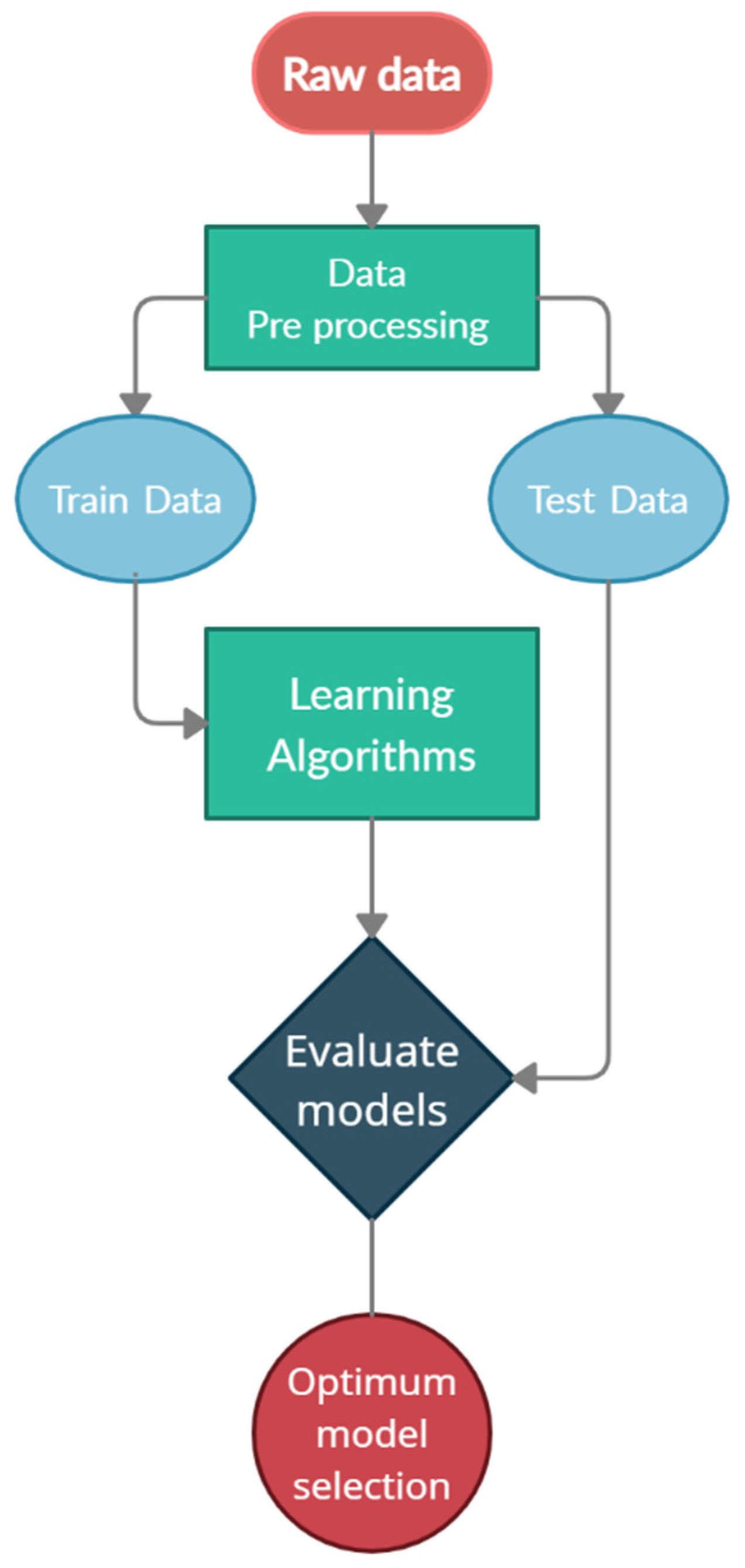
This paper uses machine ML, a novel approach known as a subfield of AI methods, which can be a beneficial approach to best fit environmental conditions and work situations to optimize fleet management and attain an adequate output. While fleet management is related to several factors and procedures, ML methods consider work situations, like routes, types of machinery, time, and weather conditions. Furthermore, these methods also help planners to make reliable and accurate predictions. Considering that this method uses historical data, one can be assured that the results of the method can be updated. On the other hand, with the progression of time and the adding of more data, the accuracy of the algorithms increases. Also, in this method, in contrast to other initiatives, the planning can be updated by considering various situations, even the difference in plant demand in a short time that does not require any costs for the mining department. In addition, this method can be used to predict machinery in the short and long terms.

2. Machine Learning (ML)

ML has become one of the most critical topics within development organizations looking for innovative ideas to leverage data assets to help the business gain a new level of understanding. ML is a form of AI that enables a system to learn from data, rather than through explicit programming. Resurging interest in ML is due to the growing volumes and varieties of available data, and the fact that ML’s computational processing is cheaper and more powerful, and provides affordable data storage. Machines that learn can more quickly highlight or find patterns in data that human beings would have otherwise missed. Consequently, ML techniques can be used to enhance humans’ abilities to solve problems and make informed inferences on a wide range of problems. ML techniques are divided into three sections, each of which has individual performance: supervised learning, unsupervised learning, and reinforcement learning. ML uses various algorithms that iteratively learn from data to improve and describe data, and predict outcomes. As the algorithms ingest training data, it is possible to produce more precise models based on that data. An ML model is the output generated when a machine learns by a learning algorithm with data. Then, when the predictive model is provided with data, it predicts based on the data that trained the model [20]. In this paper, five regression techniques from supervised learning are employed.

Figure 1 illustrates the flowchart of the optimum model selection operation using the ML algorithms. As shown in Figure 1, all collected data was firstly sorted and standardized. based on needs, so that machine learning algorithms could read and understand it. Then these datasets were divided into two parts, including training and evaluation data. After this division, the training data was entered as inputs to different algorithms to train the machine. After training, the values predicted by the algorithm and the actual outputs of the evaluation section were compared, and the accuracy of the algorithm was estimated. Finally, the algorithm with the highest accuracy level was selected as the optimal algorithm to continue the process.

3. Studied Site

Zenouz kaolin mine is located near Zenouz city, approximately 15 km North of Marand city of East Azerbaijan, Iran. Given that the Zenouz kaolin mine is one of the biggest in the area, it contributes significantly to the local economy. The key factor in the amount of revenue is transportation costs. In addition, kaolin is one of the important components of the ceramic, insulation, and tile industries and has a crucial impact on the entire production process. Therefore, the success and longevity of this mine is important ensure the survival of client enterprises.

The mainstay of innovation today are research and development operations using advanced technology that raise the added value of an industry sector. This study’s goal was to provide industries, that have primary costs of raw material production which are tied to transportation expenses, with a rapid, effective, persuasive, and useful technique.

Zenouz kaolin mine is the largest kaolin mine in the Middle East, producing approximately 1,700,000 tonnes of raw kaolin and supplying nearly 70% of the kaolin in the region. This mine includes five working zones. Each zone has its own individual characteristics and processing plant demands. The mining method in this mine is open-pit mining, and kaolin is extracted by blasting, loaded by various types of excavators, and hauled by trucks to the processing plant and low-grade stockpiles.

Figure 2 shows the location of different zones and stockpiles.

Data Collecting:

By collecting five years of records, from May 2017 to May 2021, in seven different divisions, the 1975 data were regarded as machine learning input data. The data were converted into numerical data to transform descriptive data into something understandable and agreeable to machines. These seven categories and their related numerical forms are presented as follows:

3.1. Month

This information was taken into account because the amount of minerals hauled varied by month. Therefore, numbers 1 to 12 were allocated to the data for January to November, as shown in

Table 1. Months and their related numerical values.

Month	Encoded Data	Month	Encoded Data	Month	Encoded Data
January	1	May	5	September	9
February	2	August	6	October	10
March	3	June	7	November	11
April	4	July	8	December	12

. On the other hand, due to the fact that months are cyclic variables, the values were encoded by transforming the data into two dimensions using a sine and cosine transformation.

3.2. Weather Condition

Weather conditions influence the operation of the hauling systems because operators and equipment perform differently in various weather conditions. Since weather conditions affect the amount of ore haulage, related data on this factor were collected and divided into five situations, shown in

Table 2. Weather conditions and related encoded data.

Weather Condition	Encoded
Cloudy	(1,0,0,0,0)
Foggy	(0,1,0,0,0)
Rainy	(0,0,1,0,0)
Snowy	(0,0,0,1,0)
Sunny	(0,0,0,0,1)

.

3.3. Season

According to experimental observations, the amount of mineral transportation varied in different seasons. Hence, this parameter was also analyzed for better consideration as training data and is presented in

Table 3. Seasons and related encoded data.

Season	Encoded
Spring	(1,0,0,0)
Summer	(0,1,0,0)
Fall	(0,0,1,0)
Winter	(0,0,0,1)

.

3.4. Weekday

Due to several spatial and temporal constraints, truck drivers’ weekend driving behavior is expected to differ considerably from their weekday driving style. Thus, the weekdays were also considered and evaluated in

Table 4. Weekdays and related encoded data.

Weekday	Encoded
Monday	0
Tuesday	1
Wednesday	2
Thursdays	3
Friday	4
Saturday	5
Sunday	6

.

3.5. Number of Trucks

In Zenouz kaolin mine, two models of trucks, Sahand-WD615 and Mercedes-Benz-OM335, are used, and the carrying capacity of each is 26 tons on average. The number of trucks that haul minerals from different zones to stockpiles was also considered as analyzable data for machine learning.

3.6. Routes

Zenouz mine complex includes six loading spots and two delivery points (see Figure 2). Regarding the distances of these zones from the stockpiles, and considering the production plan, this parameter was separated into nine divisions, shown in

Table 5. Routes and related abbreviations and encoded data.

Route	Abbreviation of Routes	Encoded
LG-stockpile to plant	LGP	(1,0,0,0,0,0,0,0,0)
Mine 1 to plant	M1P	(0,1,0,0,0,0,0,0,0)
Mine 1 to LG-stockpile	M1LG	(0,0,1,0,0,0,0,0,0)
Mine 2 to plant	M2P	(0,0,0,1,0,0,0,0,0)
Mine 2 to LG-stockpile	M2LG	(0,0,0,0,1,0,0,0,0)
Mine 3 to plant	M3P	(0,0,0,0,0,1,0,0,0)
Mine 4 to plant	M4P	(0,0,0,0,0,0,1,0,0)
Mine 4 to LG-stockpile	M4L	(0,0,0,0,0,0,0,1,0)
Super Mine1 to plant	SP	(0,0,0,0,0,0,0,0,1)

.

3.7. Loader Types

Since different types of excavator load trucks are utilized, the efficiency of these machines was investigated. Four types of excavators were used as loaders at the studied site, which were taken into account as part of the input data.

Table 6. Types of excavators and their related encoded data.

Loader Type	Encoded
Hyundai 250	(1,0,0,0)
Hyundai 320	(0,1,0,0)
Komatsu 200	(0,0,1,0)
Komatsu 220	(0,0,0,1)

displays these loaders, as well as the numerical data associated with them.

Table 7. Sample of collected data.

Row	Month	Weather Condition	Season	Weekday	No. of Tucks	Routes	Loader	Hauled Ore (tonne)
50	5	Sunny	Summer	Monday	6	M1 to plant	Hyundai 320	382.800
51	5	Sunny	Summer	Thursday	12	M1 to plant	Hyundai 320	1131.310
52	5	Sunny	Summer	Friday	18	M1 to plant	Hyundai 320	2129.650
53	5	Sunny	Summer	Saturday	18	M1 to plant	Hyundai 320	2277.940
54	5	Sunny	Summer	Wednesday	14	M4 to plant	Hyundai 320	2036.88

shows examples of the collected data and

Table 8. Encoded value of the data presented in Table 7.

Row	Month	Weather Condition	Season	Weekday	No. of Tucks	Routes	Loader	Hauled Ore (tonne)
50	5	4	2	1	6	1	1	382.800
51	5	4	2	4	12	1	1	1131.310
52	5	4	2	0	18	1	1	2129.650
53	5	4	2	2	18	6	1	2277.940
54	5	4	2	6	14	1	1	2036.88

illustrates final table after converting the data to numerical data.

4. Data Pre-Processing

4.1. Important Data

Weekdays had insignificant impacts on model learning and creation basis and had low impact rates on the learning process (see Figure 3) and this, along with the unpredictability of the weather in the long term, meant the inclusion of weekdays in the continuation of modeling was omitted. Five parameters were used as input data: season, month, number of trucks, routes, and loader types. The data was processed and validated through efficient techniques to train the machine properly.

4.2. Time Series Validator

K-fold cross-validation effectively partitions the data into K chunks, K-1 of which formed the training set R, and the last chunk served as the validation set V. Cross-validation was iterated through all combinations of assignments of chunks to R and V. This procedure was repeated for all K choices for the validation set and the performance of the model from the K runs was averaged in [21]. However, this method chose data randomly and neglect the sequence of time. So, in this paper, another effective method, namely the time series splitter, was used to split both training and validation data. Figure 4 shows how this method ran.

4.3. R² Score

The R² coefficient (Equation (1)) represents the proportion of variation in the model’s predicted result, based on its features and real data [22].

$${{\mathrm{R}}^2}_{(\mathrm{ytrue},\mathrm{ypred})}=1-\frac{\sum {\left(\mathrm{ytrue}-\mathrm{ypred}\right)}^2}{\sum {\left(\mathrm{ytrue}-\overline{\mathrm{y}}\right)}^2}=\frac{RSS}{TSS}$$

(1)

In which R² is the coefficient of determination, RSS is the sum of squares of residuals, and TSS is the total sum of squares.

5. Modeling

After collecting data, excluding insufficient data, and processing the data, 1580 and 395 data points were imported into the machine as training and test data, respectively. In ML, dozens of unique algorithms perform specialized purposes, including, regression, clustering, and classification. The amount of hauled ore was continuous data; therefore, regression methods that deliver a continuous type of data was selected in this paper. The following sections describe the validation of the five algorithms.

5.1. Linear Regression (LR)

LR is a linear approach for modelling the relationship between scalar response and one or more explanatory variables. In LR, the relationships are modeled using linear predictor functions, the unknown model parameters of which are estimated from the data [21]. By running the algorithm on the processed input data, a model with 74% accuracy was achieved. Figure 5 shows the data’s real and predicted values from numbers 50 to 150. The algorithm parameters for this method were fit intercept = True, normalize = deprecated, copy_X = True, n_jobs = None.

5.2. Decision Tree Regression (DTR)

Decision tree learning algorithms are based on heuristics, such as a greedy approach, where the tree is constructed gradually, and locally optimal decisions are made at the construction of each node [21]. By attempting this algorithm, predicted data were fitted to real data with 72% accuracy. Figure 6 compares real data, and decision tree regression algorithm predicted data. Parameters used for this algorithm were splitter = ‘best’, max_depth = 3, min_samples_split = 2, min_samples_leaf = 1.

5.3. K-Nearest Neighbors Algorithm (KNN)

K nearest neighbour algorithm is a supervised learning technique used to classify or predict new data points, based on the relationship to nearby data points [23]. Actual and predicted values using the KNN algorithm are shown in Figure 7. The accuracy of the KNN prediction was 78%. Also, the parameters of learning the algorithm to be modified were: n_neighbors = 5, weights = ‘uniform’, algorithm = ‘auto’, leaf_size = 30, n_neighbour = 7.

5.4. Random Forests (RF)

RF is a regressor consisting of a collection of decision trees. The prediction of the RF is obtained by a majority vote over the predictions of the individual trees, and, also, RF generally outperformed decision trees’ performance [21] with the implementation of this algorithm. Figure 8 shows the difference between the actual and predicted values by random forest regression algorithm for the obtained accuracy of 83%.

5.5. Gradient Boosting Decision Tree

Rather than selecting combinations of binary questions at random (like RF), gradient boosting selects binary questions that improve prediction accuracy for each new tree. This works because mistakes incurred with the training data are recorded and then applied to the next round of training data. At each iteration, weights are added to the training data, based on the results of the previous iteration. A higher weighting is applied to instances incorrectly predicted from the training data, and those correctly predicted receive less weighting. The training and test data are then compared, and errors are again logged in order to inform weighting at each subsequent round [23]. Figure 9 shows that the gradient boosting algorithm could predict the data with 85% accuracy and the parameters were learning_rate = 0.19, max_depth = 3, n_estimators = 35.

6. Model Selection

The gradient boosting algorithm was chosen as the best among the investigated algorithms. With 85% accuracy, this algorithm was used for the rest of the study after measuring the implemented algorithms to achieve an optimal model using the R² score formula. Each algorithm’s efficiency is depicted in Figure 10.

7. Ore Transport Schedule

A Mine Planning team calculates the required monthly ore production from each mine based on the processing plant’s required monthly feed.

Table 9. Ore annual haulage scheduling (ktonne).

Month	SUP. to P	M1 to P	M2 to P	M3 to P	M4 to P	M1 to LG	M2 to LG	M4 to LG	LG to P	Total Ore to the Plant
1	0	60	15	0	0	15	0	0	0	75
2	12	65	17	0	0	20	0	0	0	94
3	15	65	17	14	0	20	0	0	0	111
4	15	65	17	14	25	20	10	5	0	136
5	15	65	17	0	33	30	0	5	0	130
6	15	65	17	0	33	30	0	5	0	130
7	10	65	17	0	33	30	10	5	0	125
8	8	65	17	0	33	30	0	5	0	123
9	0	65	17	0	33	25	0	5	0	115
10	0	65	17	0	33	25	8	3	0	115
11	0	65	17	0	20	25	0	3	0	102
12	0	60	15	0	0	16	0	3	10	85
Annual ore to the plant										1341

shows the calculated monthly amount of ore from different zones.

While there are some limitations, simultaneous loading in more than three working zones is not possible. As a result, working days for different zones were planned according to Figure 11.

Table 10. Daily ore production schedule.

Month	SUP. to P	M1 to P	M2 to P	M3 to P	M4 to P	M1 to LG	M2 to LG	M4 to LG	LG to P
1	0	2000	1500	0	0	2143	0	0	0
2	1200	2097	1700	0	0	2000	0	0	0
3	1500	2097	1700	2000	0	2000	0	0	0
4	1500	2097	1700	2000	1667	2000	2000	1667	0
5	1500	2097	1700	0	2200	2000	0	1667	0
6	1500	2097	1700	0	2200	2000	0	1667	0
7	1429	2167	1700	0	2200	2000	2000	1667	0
8	1600	2167	1700	0	2200	2000	0	1667	0
9	0	2167	1700	0	2200	1667	0	1667	0
10	0	2167	1700	0	2200	1667	2000	1000	0
11	0	2167	1700	0	1333	1667	0	1000	0
12	0	2000	1500	0	0	1067	0	1000	2000

shows the required daily ore quantity to cover the processing plant’s annual demand depending on this plan.

The algorithm used 1258 individual scenarios after measuring the daily required ore amount. As a result, the minimum difference between the predicted and required data values was calculated, and the optimal fleet was selected, based on related items to this data. According to Figure 12, the machine anticipated a Hyundai 320 excavator and 19 trucks as the ideal fleet in April to transport ore from Mine 1 to the plant’s stockpiles.

The most suitable fleet was selected using 11.322 scenarios as input data for five loading points and two mineral discharge stockpiles.

Table 11. Optimum fleet to supply processing plant demands.

	Sup. to Plant		Mine1 to Plant		Mine2 to Plant		Mine3 to Plant		Mine4 to Plant		Mine1 to LG		Mine2 to LG		Mine4 to LG		LG to Plant
Month	Loader	No. of Trucks	Loader	No. of Trucks	Loader	No. of Trucks	Loader	No. of Trucks	Loader	No. of Trucks	Loader	No. of Trucks	Loader	No. of Trucks	Loader	No. of Trucks	Loader	No. of Trucks
1			H250	17	H320	10					H250	11
2	H320	9	H250	18	H320	11					H250	11
3	H320	11	H320	19	H250	11	K200	12			K220	12
4	K200	12	H320	19	H320	11	K200	12	K200	10	K220	12	K220	11	K200	11
5	K200	12	H320	19	H250	11			H320	13	K220	12			H320	12
6	K200	12	H320	19	H250	11			H320	13	K220	12			H320	12
7	H320	11	H320	19	H250	11			K200	13	H250	11	K200	11	H320	12
8	K220	10	H320	19	H250	11			K200	13	H250	11			H320	12
9			K220	21	K200	12			K200	13	H250	10			H320	12
10			H250	19	H320	11			H320	13	K220	10	K220	11	K220	9
11			K220	18	H320	11			K200	10	H250	10			K200	8
12			H320	16	K200	10			K200	6	H250	9			K200	8	H320	17

shows the best loader and number of trucks that different zones should use over the 12 months.

8. Conclusions

According to estimations, mineral transportation costs cover a large share of the operating costs and are becoming a challenge in mining management. So, implementing optimization in this operation can minimize the loss of capital costs, reduce the final price of the mineral, and increase profitability. In this paper, the ML method was used as an innovative approach to simulate operations, and was executed in the Zenouz kaolin mine to optimize fleet selection. Consequently, the Gradient Boosting Regressor, an excellent algorithm, was chosen and taught by various operational and conditional data to fit and predict the most beneficial fleet. Finally, the best daily required fleet to supply ore transportation to stockpiles was obtained by matching the processing plant ore demands and predicted values and finding the minimum difference between these values. As a result, the suggested fleet reduced truck queuing and excavators’ idle times, which account for a considerable portion of energy consumption and capital wasting.

References

1. Zhao, Y.; Sun, B.; Liu, S.; Zhang, C.; He, X.; Xu, D.; Tang, W. Identification of mining induced ground fissures using UAV and infrared thermal imager: Temperature variation and fissure evolution. ISPRS J. Photogramm. Remote Sens. 2021, 180, 45–64. [Google Scholar] [CrossRef]
2. Zheng, J.; Fu, H.; Li, W.; Wu, W.; Yu, L.; Yuan, S.; Kanniah, K.D. Growing status observation for oil palm trees using Unmanned Aerial Vehicle (UAV) images. ISPRS J. Photogramm. Remote Sens. 2021, 173, 95–121. [Google Scholar] [CrossRef]
3. Puniach, E.; Gruszczyński, W.; Ćwiąkała, P.; Matwij, W. Application of UAV-based orthomosaics for determination of horizontal displacement caused by underground mining. ISPRS J. Photogramm. Remote Sens. 2021, 174, 282–303. [Google Scholar] [CrossRef]
4. Li, Z. A methodology for the optimum control of shovel and truck operations in open-pit mining. Min. Sci. Technol. 1990, 10, 337–340. [Google Scholar] [CrossRef]
5. Lizotte, Y.; Bonates, E. Truck and shovel dispatching rules assessment using simulation. Min. Sci. Technol. 1987, 5, 45–58. [Google Scholar] [CrossRef]
6. Hashemi, S.; Sattarvand, J. Application of ARENA Simulation Software for Evaluation of Open Pit Mining Transportation Systems—A Case Study. In Proceedings of the 12th International Symposium Continuous Surface Mining—Aachen 2014, Aachen, Germany, 1 October 2014; Springer: Cham, Germany, 2015; pp. 213–224. [Google Scholar] [CrossRef]
7. Temeng, V.A.; Otuonye, F.O.; Frendewey, J.O. A Nonpreemptive Goal Programming Approach to Truck Dispatching in Open Pit Mines. Miner. Resour. Eng. 1998, 7, 59–67. [Google Scholar] [CrossRef]
8. Mena, R.; Zio, E.; Kristjanpoller, F.; Arata, A. Availability-based simulation and optimization modeling framework for open-pit mine truck allocation under dynamic constraints. Int. J. Min. Sci. Technol. 2013, 23, 113–119. [Google Scholar] [CrossRef]
9. Topal, E.; Ramazan, S. A new MIP model for mine equipment scheduling by minimizing maintenance cost. Eur. J. Oper. Res. 2010, 207, 1065–1107. [Google Scholar] [CrossRef]
10. Gu, Q.; Lu, C.; Guo, J.; Jing, S. Dynamic management system of ore blending in an open pit mine based on GIS/GPS/GPRS. Min. Sci. Technol. 2010, 20, 132–137. [Google Scholar] [CrossRef]
11. Cox, W.; French, T.; Reynolds, M.; While, L. A Genetic Algorithm for Truck Dispatching in Mining. EPiC Ser. Comput. 2018, 50, 78–93. [Google Scholar] [CrossRef]
12. Ahangaran, D.K.; Yasrebi, A.B.; Wetherelt, A.; Foster, P. Real-time dispatching modelling for trucks with different capacities in open pit mines. Arch. Min. Sci. 2012, 57, 39–52. [Google Scholar] [CrossRef]
13. Upadhyay, S.P.; Askari-Nasab, H. Simulation and optimization approach for uncertainty-based short-term planning in open pit mines. Int. J. Min. Sci. Technol. 2018, 28, 153–166. [Google Scholar] [CrossRef]
14. Baek, J.; Choi, Y. Deep neural network for predicting ore production by truck-haulage systems in open-pit mines. Appl. Sci. 2020, 10, 1657. [Google Scholar] [CrossRef] [Green Version]
15. Moradi-Afrapoli, A.; Upadhyay, S.; Askari-Nasab, H. Truck dispatching in surface mines—Application of fuzzy linear programming. J. S. Afr. Inst. Min. Metall. 2021, 121, 1–8. [Google Scholar] [CrossRef]
16. Mohtasham, M.; Mirzaei-Nasirabad, H.; Askari-Nasab, H.; Alizadeh, B. A multi-objective model for fleet allocation schedule in open-pit mines considering the impact of prioritising objectives on transportation system performance. Int. J. Min. Reclam. Environ. 2021, 35, 709–727. [Google Scholar] [CrossRef]
17. Yeganejou, M.; Badiozamani, M.; Moradi-Afrapoli, A.; Askari-Nasab, H. Integration of simulation and dispatch modelling to predict fleet productivity: An open-pit mining case. Min. Technol. Trans. Inst. Min. Metall. 2021, 131, 67–79. [Google Scholar] [CrossRef]
18. Mohtasham, M.; Mirzaei-Nasirabad, H.; Askari-Nasab, H.; Alizadeh, B. Truck fleet size selection in open-pit mines based on the match factor using a MINLP model. Min. Technol. Trans. Inst. Min. Metall. 2021, 130, 159–175. [Google Scholar] [CrossRef]
19. Upadhyay, S.P.; Tabesh, M.; Badiozamani, M.M.; Moradi Afrapoli, A.; Askari-Nasab, H. A simulation-based algorithm for solving surface mines’ equipment selection and sizing problem under uncertainty. CIM J. 2021, 12, 36–46. [Google Scholar] [CrossRef]
20. Judith Hurwitz, D.K. Machine Learning for Dummies; For Dummies: New York, NY, USA, 2018. [Google Scholar]
21. Shalev-Shwartz, S.; Ben-David, S. Understanding Machine Learning: From Theory to Algorithms; Cambridge University Press: Cambridge, UK, 2013; Volume 9781107057. [Google Scholar]
22. Raschka, S.; Mirjalili, V. Python Machine Learning; Packt Publishing: Birmingham, UK, 2019; Volume 69. [Google Scholar]
23. Theobald, O. Machine Learning for Absolute Beginners; Scatterplot Press: London, UK, 2017. [Google Scholar]
Figure 1. Optimum model selection flowchart.
Mining 02 00028 g001
Figure 2. Working zones, low-grade stockpile and processing plant stockpile locations.
Mining 02 00028 g002
Figure 3. Impact rate of each parameter on the hauled ore.
Mining 02 00028 g003
Figure 4. Time series validator performance.
Mining 02 00028 g004
Figure 5. Comparison between real data and prediction of linear regression algorithm.
Mining 02 00028 g005
Figure 6. Comparison between real data and prediction of decision tree regression algorithm.
Mining 02 00028 g006
Figure 7. Comparison between real data and prediction of K nearest neighbour algorithm.
Mining 02 00028 g007
Figure 8. Comparison between real data and prediction of the random forest regression algorithm.
Mining 02 00028 g008
Figure 9. Comparison between real data and prediction of gradient boosting regression algorithm.
Mining 02 00028 g009
Figure 10. Implemented algorithms accuracy in percent.
Mining 02 00028 g010
Figure 11. Working zones daily ore hauling schedule plan.
Mining 02 00028 g011
Figure 12. Optimum loader type and number of trucks selection.
Mining 02 00028 g012