1. Introduction
A mining operation contains several factors that affect its efficient extraction of resources. One such factor is fragmentation size, a key parameter across almost all of the stages of production from mine (drill, blasting, haulage, etc.) to mill (mineral processing). Several studies have explored the effect of fragmentation size on other factors such as drilling and blasting cost [
1] and the performance of crushing and grinding circuits [
2,
3]. Therefore, it can be considered that it is vital for companies to continuously monitor fragmentation size and make necessary changes to mine planning and execution to keep the fragmentation size that is most beneficial to the operation as a whole. Traditionally, methods such as manual sieving, boulder counting, and visual estimation have been used for fragmentation size measurement. However, due to the generally large amount of material being mined and its innately heterogeneous nature, difficulties arise from using traditional methods. In addition, limitations on sampling as well as bias make these methods relatively inefficient [
4]. As such, there exists a need for a quick and accessible method of rock fragmentation size distribution determination that can surmount the limitations of physical sampling and laboratory analysis. A currently used digital solution to this problem is to employ image-based particle size analysis software. Commercial products such as WipFrag [
5,
6] and Split Desktop [
7,
8] use images of muckpiles or orthomosaics to measure fragmentation size distribution, where the conventional studies use 2D information and the 3D size estimation accuracy is relatively low.
A 3-Dimensional Fragmentation Measurement (3DFM) system was developed that uses 3D photogrammetry to measure fragmentation size distribution at accuracies greater than that of conventional methods [
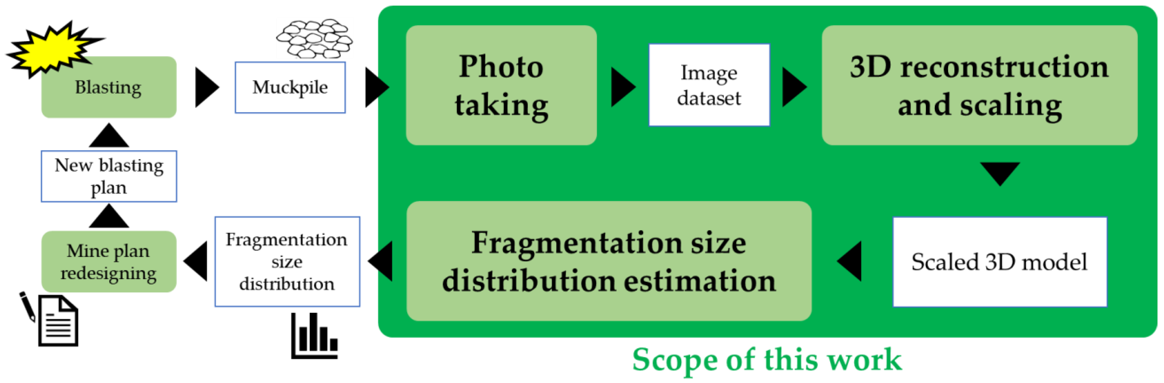
9]. The 3DFM extracts the fragmentation sizes from a 3D muckpile model, which facilitates accurate fragmentation size distribution measurement without scale objects and eliminates the need for excessive manual editing. Furthermore, a representative fragmentation of an entire blasting shot can easily be analyzed by generating a 3D model of an entire blasted muckpile. A workflow for this system when applied to a mining operation, and scope of this work, is shown in
Figure 1.
The developed system is divided into stages, utilizing multiple computational techniques in order to achieve its purpose. In a hypothetical application of the system, pictures of the muckpiles from the products of blasting are taken. The sizes of muckpiles vary considerably depending on the specifications of the hauling equipment as well as the mine plan that the operation employs. In situations where the muckpiles are too large or have parts inaccessible to photo-taking, the system can reconstruct only a representative slice of the muckpiles. The images are then processed in a high-power computer by a sequence of 3D imaging techniques that will ultimately output a scaled 3D model of the muckpiles in the form of a point cloud. The dimensional data can be used to compute the fragment size distribution of the muckpiles. Using this information, the blasting product can be judged if it is up to the expected specification. Adjustments are then made to the blasting design, such as the amount and type of explosive and blasting patterns to achieve the required distribution.
Scaling is a critical component of fragmentation size distribution measurement using photogrammetry as it will directly determine the accuracy of the size estimation. In creating a 3D model, extrinsic data such as ground truths are needed to create a properly-scaled reconstruction of the scene. Several methods are used to resolve scale in photogrammetry. Most of these methods have the same basic idea in that once the exact distance between at least two different points in a scene as a ground truth is known, a scale factor can be applied to the 3D model. One way to do this is to include an object of known length, such as scale bars, in the scene. In larger applications such as aerial mapping, GCPs (Ground Control Points) are used, marked points of known absolute or relative coordinates.
A previous work by authors [
10] proposed a method using GNSS (Global Navigation Satellite System, such as GPS) to get absolute (but rough) camera positions for scaling muckpile fragmentation. The authors showed the potential of the fragmentation size distribution estimation method using rocks similar to muckpiles in the previous work, but the verification test with actual muckpiles and fragmentation size distribution estimation remained an issue.
This paper validates the method’s effectiveness through practical experiments using actual muckpiles generated in a quarry site, and show that the method can be applied to fragmentation size distribution measurement.
2. Muckpile Scaling by GNSS-Aided Photogrammetry
2.1. Structure-from-Motion-Multi-View-Stereo (SfM-MVS)
Structure from Motion (SfM) has been collectively defined as the photogrammetric technique [
11], the process [
12], as well as the tools [
13] used to generate 3D models from 2D images taken at different angles. It has been developed since the 1980s, resulting in various applications such as photogrammetric surveys, virtual reality model reconstruction, determination of camera motion [
14], and odometrical scale estimation [
15]. Compared to traditional photogrammetry, where the calculation is more direct, SfM uses repeating algorithms to identify matching features in a set of overlapping images, and use these matched features to calculate camera location and orientation [
13]. SfM can be computed in several ways, depending on numerous factors such as camera type, image ordering, capture format, and more.
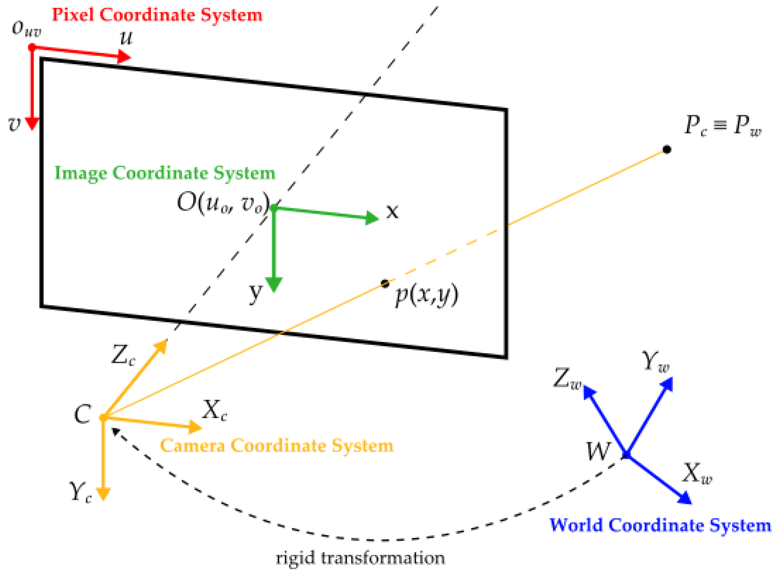
Mathematically, SfM can be described as the conversion of four coordinate systems, illustrated in
Figure 2:
- i.
Image pixel coordinate system, which concerns the pixels on the 2D image.
- ii.
Imaging plane coordinate system, which lies on the same plane of the previous system, but whose origin is the plane’s intersection with the camera’s optical axis.
- iii.
Camera coordinate system, which concerns a pinhole camera’s point of view of the image.
- iv.
World coordinate system, which is a reference system to describe the position of the camera and the objects being taken pictures of.
The conversion of these four coordinates systems can be described by Equation (1). The
and
describe the axes in the imaging planes. The
and
are the coordinates of the origins of the imaging plane in the pixel coordinate system. The
and
represent the physical size of each pixel in the image in the imaging plane (zoom ratio). The
describe the focal length, which is the distance from the optical center of the camera to the pixel plane. The
and
describes the rotational and translational vectors that relate the camera and the world coordinate systems. The
,
, and
are the actual coordinates of a point in the world coordinate system.
Equation (1) represents the fact that in order to estimate the position of a point in the real world, the external parameter matrix of the camera (i.e., and ) needs to be measured first. Once is known, the relative position of the object in the world coordinate system can be estimated, and once t is known, the absolute position can also be acquired. Basic SfM can relatively estimate and .
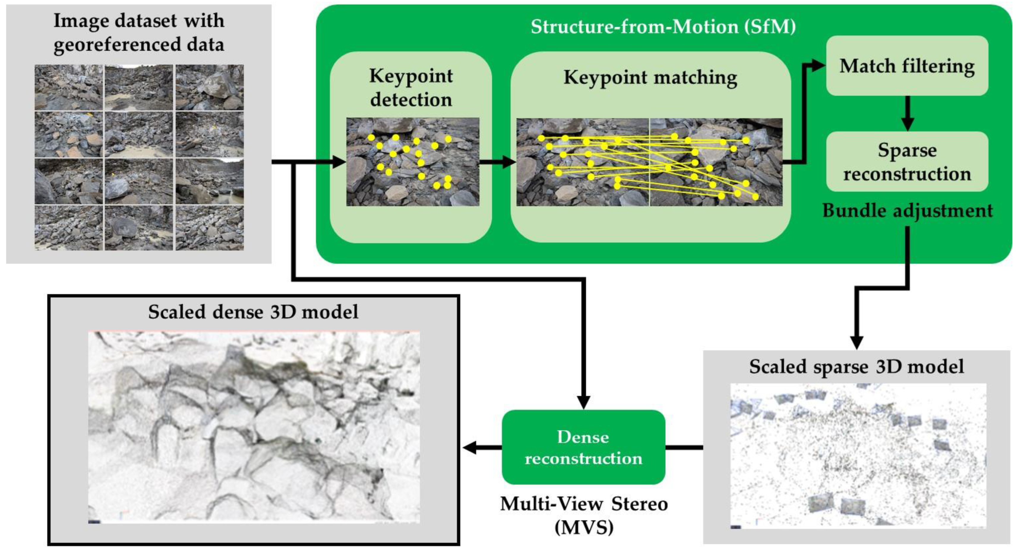
It can be inferred that there is no single correct workflow or process in the conversion of 2D images into models. However, key processes are present in almost all applications of the method, as shown in
Figure 3. Firstly, an image dataset must be taken by cameras with a GNSS receiver. As many images as possible from various viewpoints should be taken because the number of images and variation of viewpoints effect the accuracy of the result of 3D reconstruction. SfM process is composed of keypoint detection, keypoint matching, matched filtering (filtering valid corresponding points), and sparse reconstruction (bundle adjustment for 3D model with point cloud). In the bundle adjustment step, a scaled sparce 3D model is generated using the georeferenced data in the input. By combining texture information and the scaled sparse 3D model through SfM and MVS processes, the scaled and dense 3D model can be obtained.
2.2. GNSS-Aided Scaling
The study proposes a method that makes use of GNSS (Global Navigation Satellite System) data to create scaled 3D models without the need for post-reconstruction rescaling. GNSS positional data and its sub-systems such as GPS, Beidou [
16], GLONASS (GLObal NAvigation Satellite System) [
17], and QZSS (Quasi-Zenith Satellite System) [
18] can be utilized. A previous study was performed with regards to using GPS in reconstruction, but mostly in the context of UAV (Unmanned Aerial Vehicle) Mapping [
19]. This study aimed to develop a system without needing ground truth data such as GCPs to create a properly scaled 3D model of muckpiles. This would aid greatly in the fragmentation size distribution measurement of muckpiles using photogrammetry.
It is a known fact that an inherent error exists within GNSS and its subsets, and even high-end geodetic GNSS receivers have errors in the centimeter range [
20]. For this study, a smartphone is used as a GNSS receiver for the digital camera. This decision is due to the end goal of this research which is to be able use both image data and GNSS data from a smartphone, as this practicality can be important in a mining operation environment. This comes at a drawback to the GNSS accuracy, as recreational-grade GNSS chips like those found in smartphones typically have errors in the meter range [
21]. To overcome this error, the study proposes to make use of an increasing number of georeferenced images to statistically decrease the scaling error of the constructed 3D model.
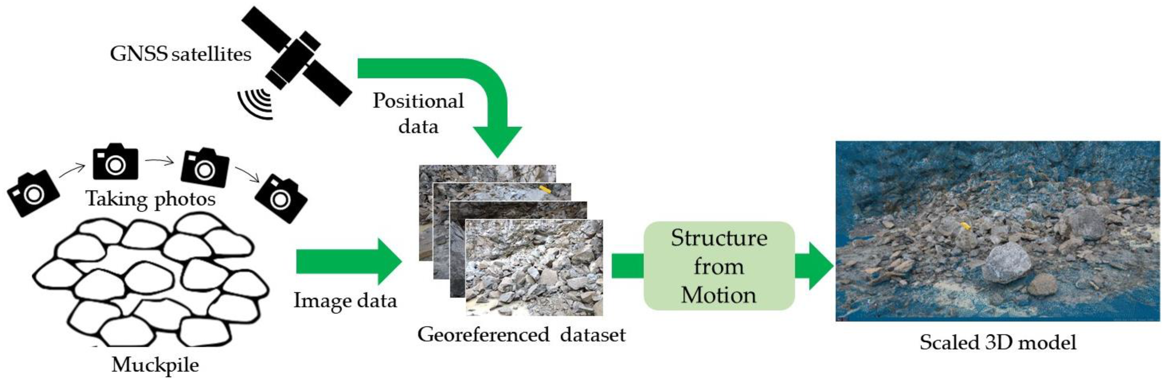
Figure 4 shows a general overview of the proposed system for this study. Utilizing a smartphone’s built-in GNSS receiver, GNSS data can be logged and sent to a camera. At the moment an image is taken, GNSS data can be embedded into the image’s metadata.
Bundle adjustment is an essential process of SfM. In the bundle adjustment phase, the previous and imperfect solutions regarding camera positions and 3D features of the scene are refined [
22]. More specifically, bundle adjustment is a nonlinear minimization procedure that jointly optimizes camera parameters and point position by minimizing the reprojection error between the image locations of observed and predicted image points. This minimization is done using nonlinear least squares algorithms [
23]. Numerous studies have been done since its inception in the 90′s regarding bundle adjustment, with most of the research going into reducing its computational burden and accelerating the problem-solving process [
24]. One such proposition is the fusion of positional data and bundle adjustment, with GNSS data being used as constraints for solving reprojection errors [
25]. This concept is what this research aims to use to produce accurately-scaled 3D reconstructions of muckpiles. GNSS data are used to provide position and covariance estimates for the bundle adjustment process. The nominal form of these solutions is:
where
is the position of the GNSS receiver,
denotes the camera position, and
is the rotational matrix that aligns camera and mapping space axes, and
is the difference between the GNSS receiver and camera position. The
and
denote bias and drift terms and are included to account for data inconsistencies and the inherent errors that exist within GNSS. A previous study [
26] applied GNSS-assisted terrestrial photogrammetry to model coastal areas without the use of GCPs. With bundle adjustment being an error minimization problem with multiple factors, weights can be assigned to them, as is the case in the study’s SfM workflow.
3. Evaluation Experiment in a Real Mine Site
For this experiment, actual muckpiles found in an active mining (quarry) site are recreated in 3D space. The aim of this experiment is to assess the performance of GNSS-aided photogrammetry in a practical application in an open mining environment.
The figures in this section are labeled “CGI” (Computer Generated Image) or “Photo” (real photo) in the lower left corner of each figure.
3.1. Experimental Site
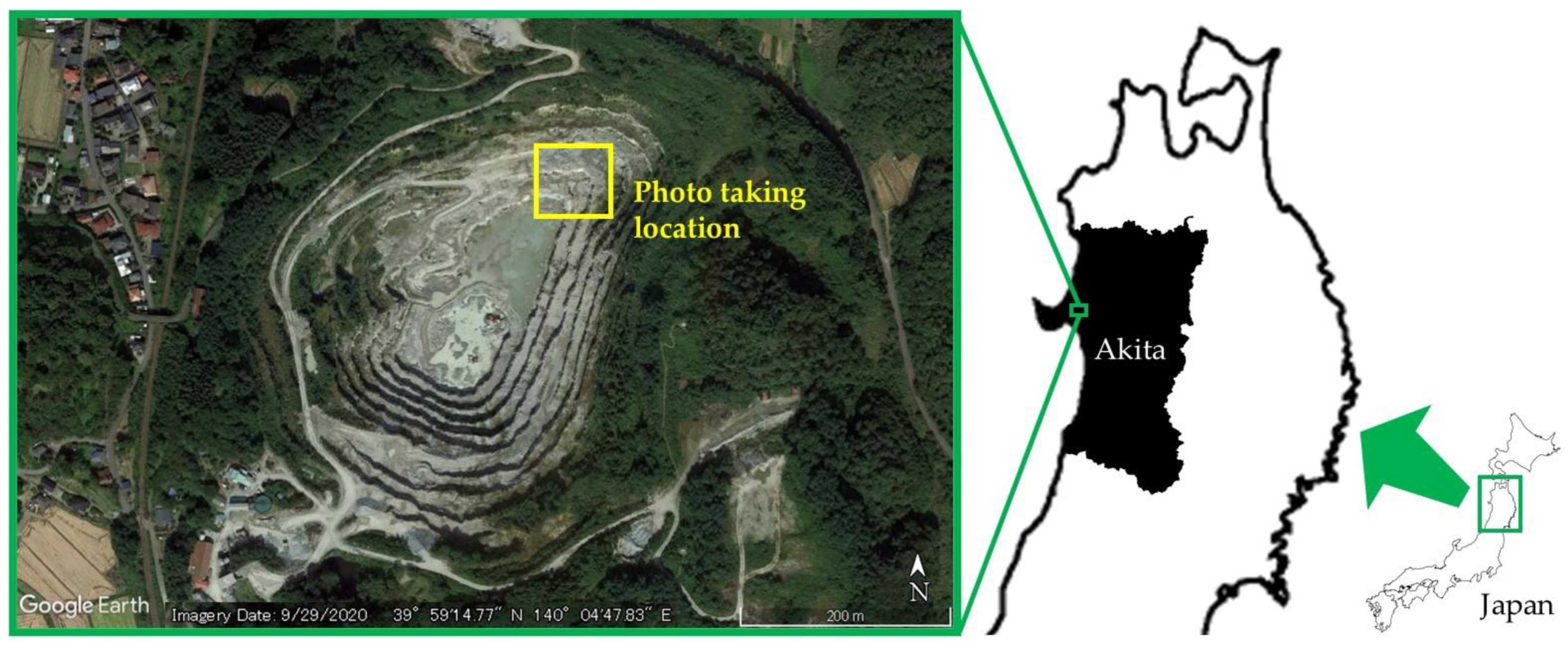
The site chosen for this experiment was the Mikurahana Quarry Site of TOSEKI MATERIAL Inc.
https://www.materiaru.jp/ (accessed on 12 June 2022), found in Hachirogata-town in Akita Prefecture, Japan, and the experiment was performed on 15 November 2021. The muckpiles were composed mainly of limestone and fragments that were generally large, with fragments as large as 2 m wide in its largest dimension. Satellite imagery is shown in
Figure 5 to provide locational context for the quarry and the muckpiles in question.
3.2. Experiment with Real Muckpiles
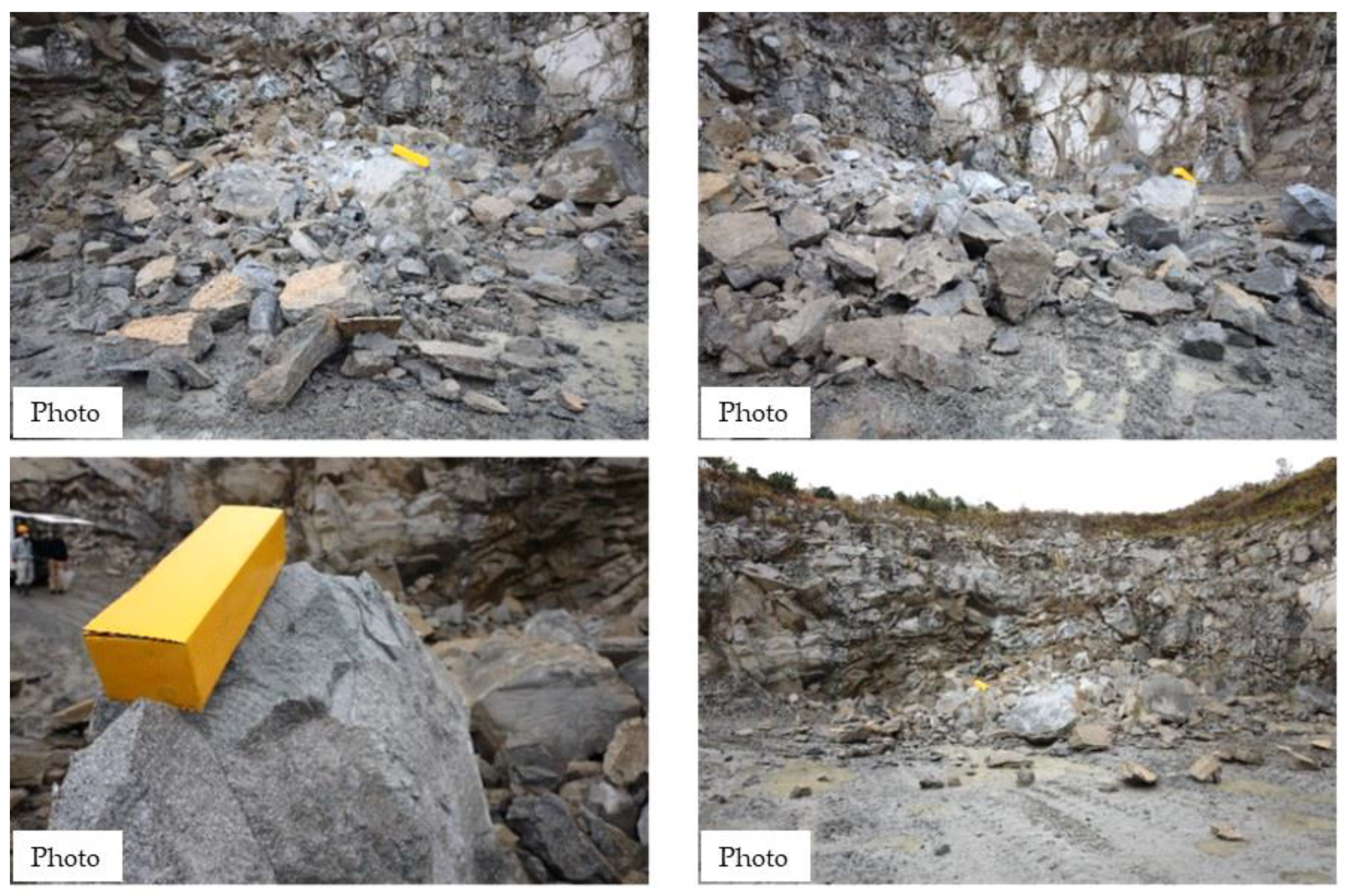
A total of 400 images of the muckpiles were taken from varying angles facing the muckpiles using a smartphone (Xiaomi Mi 9T Pro) with a GNSS receiver on. Each image size is 4464
2976 pixels. Sample images are shown in
Figure 6, which also feature the yellow cardboard box that was used as an absolute reference for scaling error. The box measures 15 cm
15 cm
cm, with the 60 cm-long side used for measuring scaling error.
3.3. Results of 3D Reconstruction and Scaling
Using 3DF Zephyr (version 6.010) [
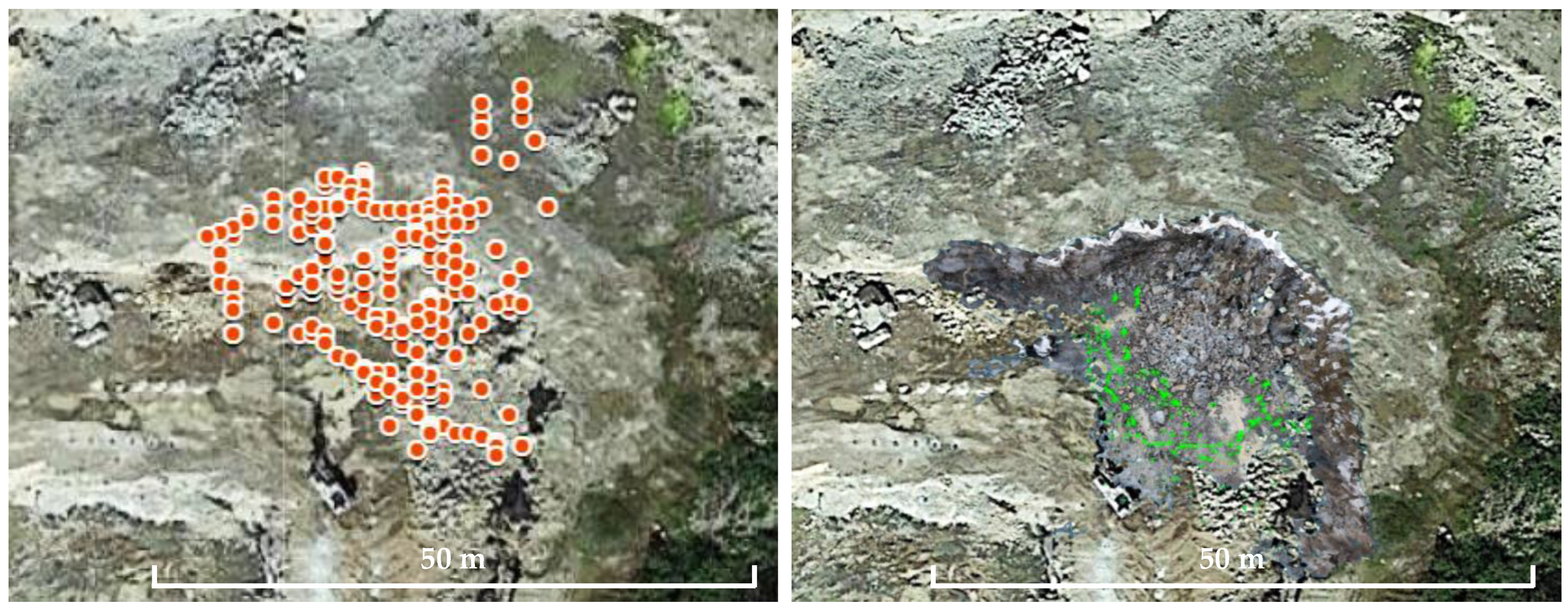
27], a 3D photogrammetry software, the images are used to create 3D models at different image numbers, namely 50, 100, 200, and 400 images. The camera positions, measured by GNSS and by SfM, are shown in
Figure 7. The red dots in the left figure represent photo-taking positions obtained using GNSS, and green objects in the right represent actual photo-taking positions measured by SfM. The figure on the right was created by manually superimposing an orthorectified image on a satellite image. The orthorectified image was generated by a 3D model obtained by SfM. We tried to take as many images as we could from various viewpoints, as
Figure 7 shows.
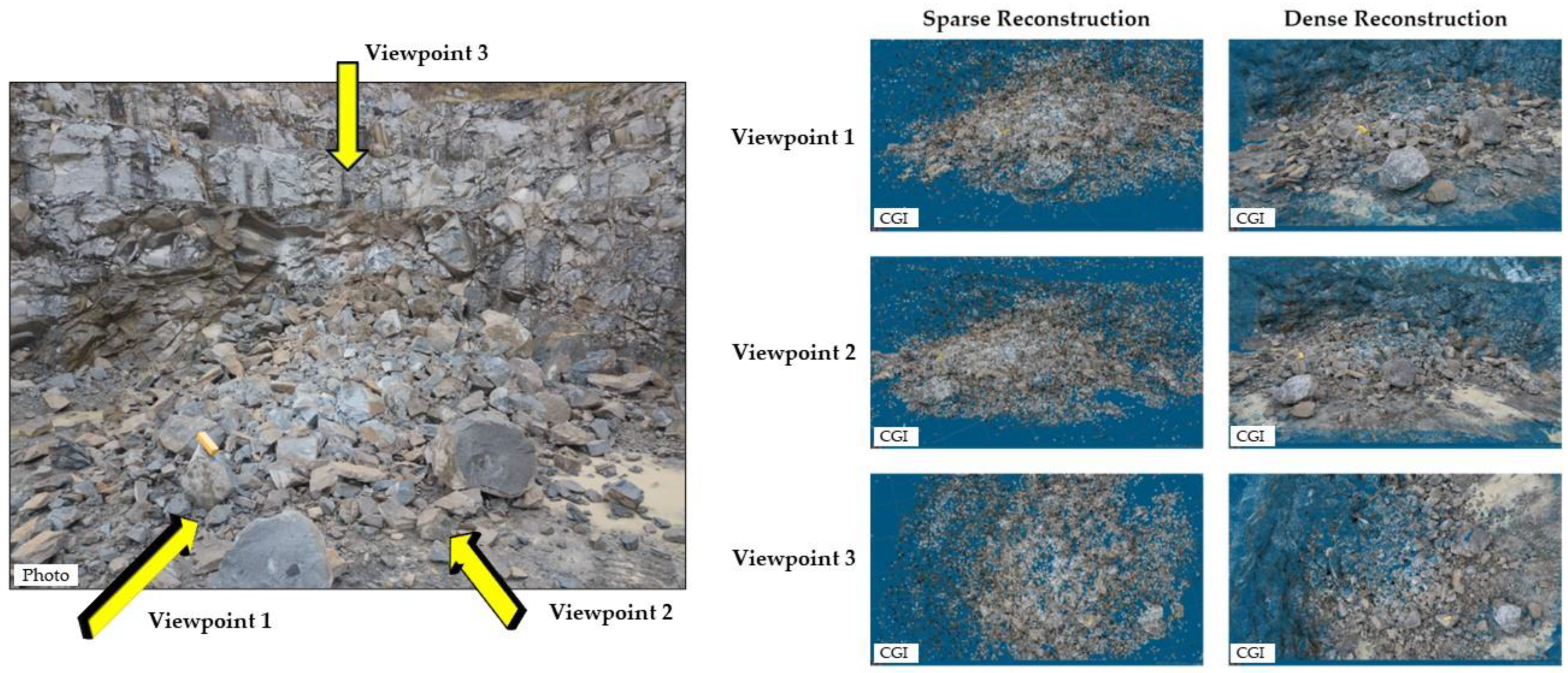
The scaling error of each model with respect to the yellow box is measured and plotted in a graph to observe the relationship between scaling error and image number. The sparse and dense reconstruction of the muckpiles at 400 images is shown in
Figure 8 at different angles for reference. A mesh reconstruction featuring measurement of the yellow box in 3DF zephyr is also shown in
Figure 9.
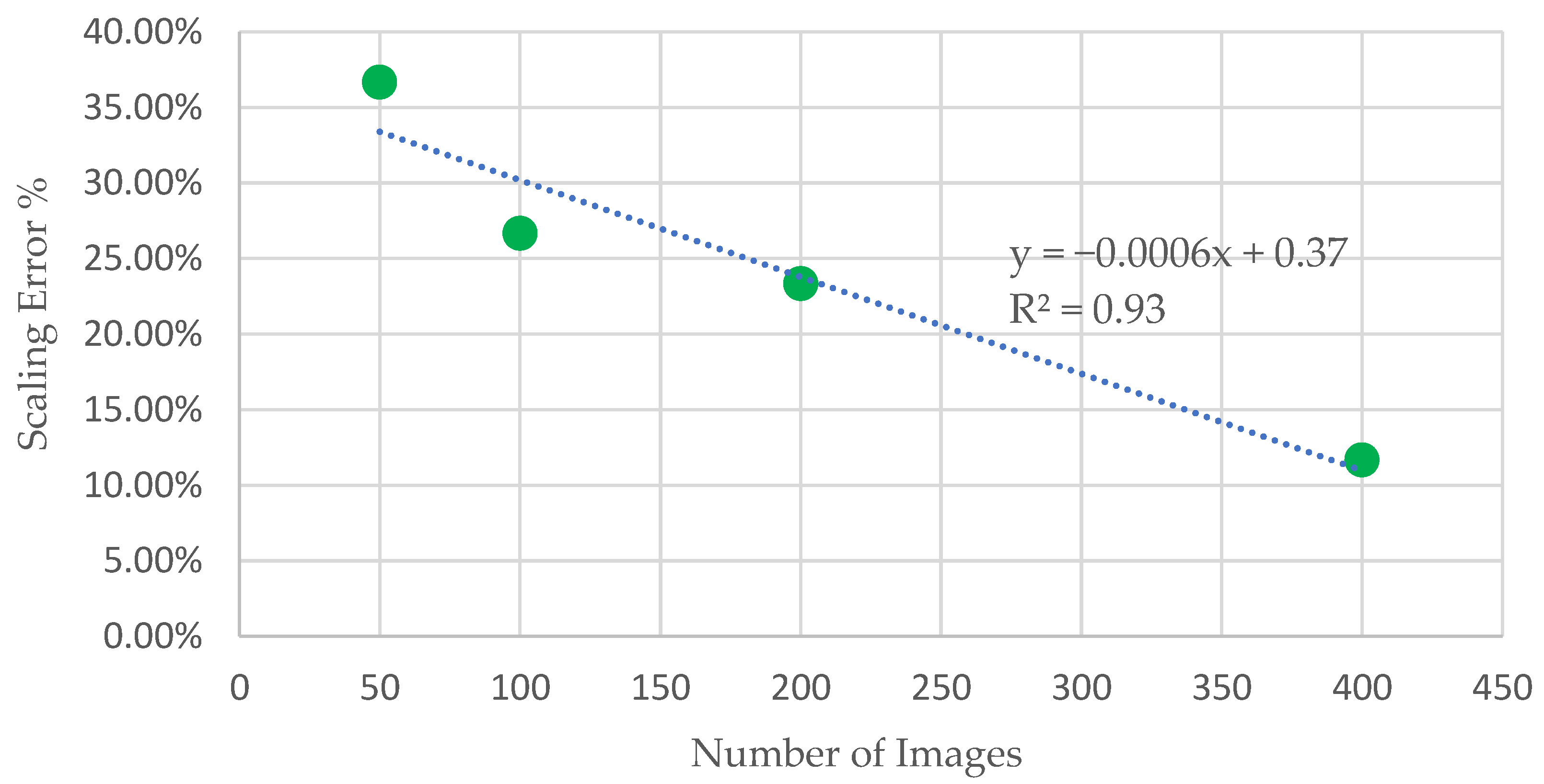
As shown in
Table 1 and
Figure 10, there is a trend that at an increasing number of images used in reconstruction, the difference from the real measurement decreases. This result, as with the previous experiments, lends more credence to the hypothesis that using more images for reconstruction has the tendency to lessen scale error in 3D models, with a relatively linear relationship between image number and scaling error as shown by the trendline with an R-value of 0.93. It is noted, however, that the improvement in scaling error by increasing the number of images is lessened, as the scaling error at using only 50 images is already 36.67%, which is much higher than when using 50 images in the other experiments. The study hypothesizes that this is due to the lack of vegetation in the area, which improved the GNSS accuracy. The study achieved 11.7% scaling error at 400 images, which is close to the extrapolated 10% scaling error at 400 images in the previous experiment on monuments [
10]. The error is comparable or more accurate than WipFrag [
5,
6].
3.4. Muckpile Fragmentation Size Distribution Estimation
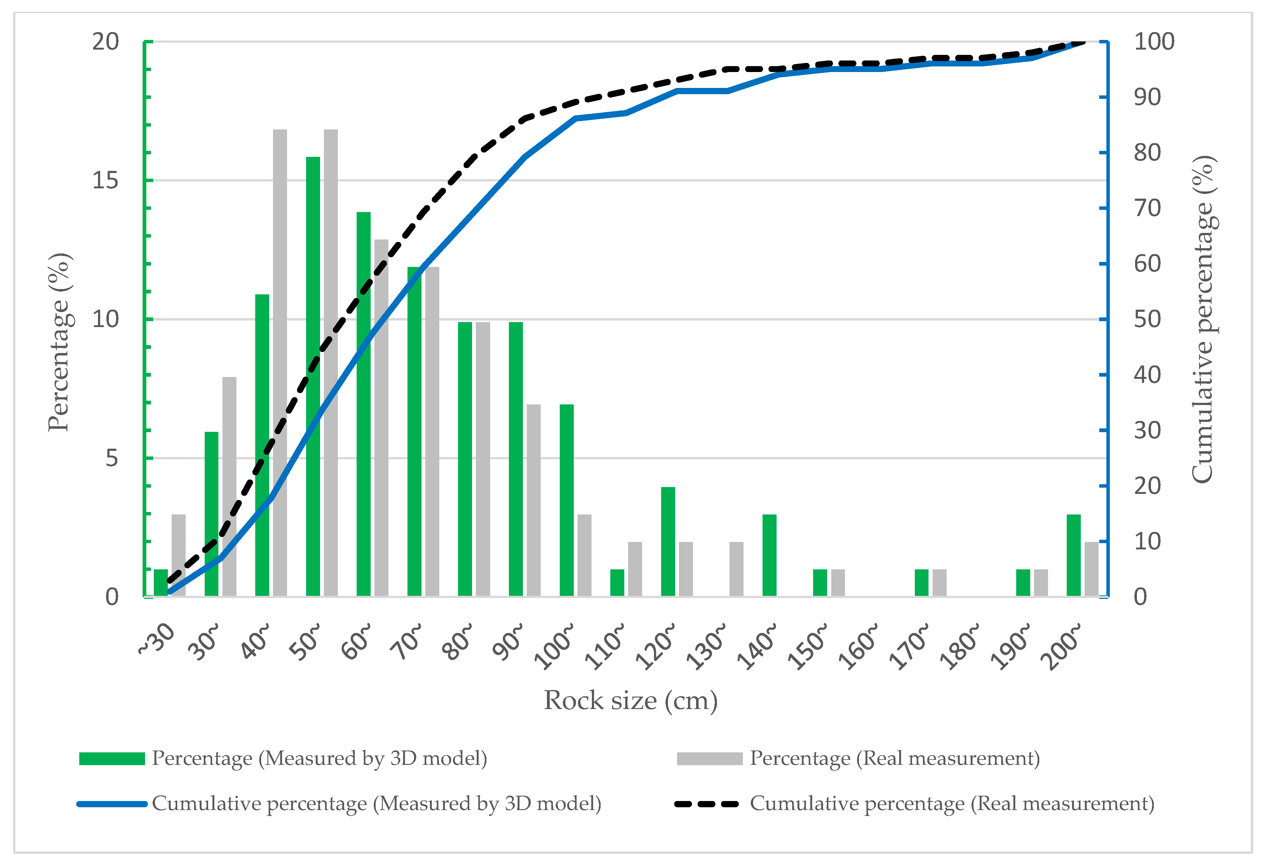
In the previous chapters, it was confirmed that scaling by GNSS-aided 3D photogrammetry is effective for actual muckpiles. In this chapter, based on the scaling results, we measured the muckpile size distribution of actual muckpiles. The results of manually measuring the muckpile size distribution of the generated 3D model of muckpiles are shown in
Figure 11. Green bars represent the percentage of each rock size measured by the 3D model, and the gray bars represent that measured by real measurements. The blue line represents the cumulative percentage of rock size measured by the 3D model, and the black dotted line represents that measured by real measurements.
Figure 11 shows that the proposed method achieved a close result to the real measurements. Referring to the result, we concluded that it is possible to measure the muckpile fragmentation size distribution in an actual quarry.
Although it is difficult to count rocks that are hidden from view by other rocks, it is possible to count all large rocks that require heavy machines to transport. Scaling of very small rocks (a few centimeters) is also difficult due to the resolution of the camera, but this is expected to improve as camera performance improves. Many and various viewpoints of photos should be taken for improving the accuracy. It is hard to achieve by handheld cameras, but it can be easier with videos by drone. An end-to-end fragmentation size distribution estimation system using drones is one of the ultimate goals of this study.
4. Conclusions
This paper showed that the method of creating an accurately scaled 3D model by constraining camera positions through georeferenced images as input for SfM can be applied to real muckpiles and can be used to measure the fragmentation size distribution. Monitoring fragmentation size is an important procedure in optimizing mining operations that perform blasting. In recent years, a new method that involves using 3D photogrammetry to measure fragment sizes has been developed that has the potential to surpass traditional techniques. For this particular process to be accurate, a method for properly scaling 3D models with georeferenced images using GNSS was investigated. An experiment was performed on actual muckpiles in the Mikurahana quarry to test the system’s accuracy in a practical application. Three-dimensional reconstructions were created at image numbers of 50, 100, 200, and 400 limestone muckpiles, and the scaling error was measured and graphed against the image number. It also showed a linear pattern with an R-squared value of 0.93. The scaling error decreases with increasing image number, albeit at a lower ratio than has been hypothesized due to the lack of interference from vegetation and buildings.
Two observations can be drawn from the experimental result: (1) increasing the number of georeferenced images in SfM will incrementally improve the scaling error of the reconstruction. These observations can help improve scale accuracy in GNSS-aided 3D fragmentation measurement; and (2) the proposed method can be applied to actual muckpiles at real mine sites. These results show examples of improving the scaling aspect of 3D fragmentation measurement systems without the use of GCPs or manual scales, specifically in surface mines where GNSS data are generally readily available. This shows that monitoring the fragmentation distribution can potentially be performed using just a camera and GNSS-enabled devices, such as smartphones or drones.
Author Contributions
Conceptualization, H.T., Z.P.L.T. and H.D.J.; methodology, H.T. and Z.P.L.T.; software, H.T. and Z.P.L.T.; validation, H.T., H.I. and Z.P.L.T.; formal analysis, N.O.; investigation, H.T. and N.O.; resources, N.O.; data curation, H.T. and Z.P.L.T.; writing—original draft preparation, H.T., Z.P.L.T. and H.I.; writing—review and editing, H.I. and Y.K.; visualization, H.T. and Z.P.L.T.; supervision, H.D.J., I.K., T.A. and Y.K.; project administration, Y.K.; funding acquisition, Y.K. All authors have read and agreed to the published version of the manuscript.
Funding
This research received no external funding.
Data Availability Statement
Not applicable.
Acknowledgments
The dataset was taken in the Mikurahana Quarry Site of TOSEKI MATERIAL Inc.
https://www.materiaru.jp/ (accessed on 12 June 2022).
Conflicts of Interest
The authors declare no conflict of interest.
References
- Afum, B.O.; Temeng, V.A. Reducing Drill and Blast Cost through Blast Optimisation—A Case Study. Ghana Min. J. 2015, 15, 50–57. [Google Scholar]
- Kanchibotla, S.S.; Valery, W.; Morrell, S. Modelling Fines in Blast Fragmentation and Its Impact on Crushing and Grinding. In Proceedings of the Explo ’99—A Conference on Rock Breaking, Kalgoorlie, Australia, 7–11 November 1999; The Australasian Institute of Mining and Metallurgy: Kalgoorlie, Australia, 1999; pp. 137–144. [Google Scholar]
- Valery, W.; Morrell, S.; Kojovic, T.; Kanchibotla, S.S.; Thornton, D.M. Modelling and Simulation Techniques Applied for Optimisation of Mine to Mill Operations and Case Studies. In Proceedings of the VI Southern Hemisphere Meeting on Mineral Technology, Rio de Janeiro, Brazil, 27 May–1 June 2001. [Google Scholar]
- Nefis, M.; Talhi, K. A Model Study to Measure Fragmentation by Blasting. Min. Sci. 2016, 23, 91–104. [Google Scholar]
- Palangio, T.C.; Franklin, J.A.; Maerz, N.H. WipFrag—A Breakthrough in Fragmentation Measurement. In Proceedings of the 6th High-Tech Seminar on State of the Art Blasting Technology, Instrumentation, and Explosives Applications, Boston, MA, USA; 1995; p. 943. Available online: https://scholarsmine.mst.edu/geosci_geo_peteng_facwork/1261/ (accessed on 12 June 2022).
- Maerz, N.H.; Palangio, T.C.; Franklin, J.A. WipFrag Image Based Granulometry System. In Measurement of Blast Fragmentation; Routledge: Abingdon, UK, 1996. [Google Scholar]
- Kemeny, J.M. Practical Technique for Determining the Size Distribution of Blasted Benches, Waste Dumps and Heap Leach Sites. Min. Eng. 1994, 46, 1281–1284. [Google Scholar]
- Kemeny, J.; Mofya, E.; Kaunda, R.; Lever, P. Improvements in Blast Fragmentation Models Using Digital Image Processing. Fragblast 2002, 6, 311–320. [Google Scholar] [CrossRef][Green Version]
- Jang, H.; Kitahara, I.; Kawamura, Y.; Endo, Y.; Topal, E.; Degawa, R.; Mazara, S. Development of 3D Rock Fragmentation Measurement System Using Photogrammetry. Int. J. Min. Reclam. Environ. 2020, 34, 294–305. [Google Scholar] [CrossRef]
- Tungol, Z.P.L.; Toriya, H.; Owada, N.; Kitahara, I.; Inagaki, F.; Saadat, M.; Jang, H.D.; Kawamura, Y. Model Scaling in Smartphone GNSS-Aided Photogrammetry for Fragmentation Size Distribution Estimation. Minerals 2021, 11, 1301. [Google Scholar] [CrossRef]
- Westoby, M.J.; Brasington, J.; Glasser, N.F.; Hambrey, M.J.; Reynolds, J.M. ‘Structure-from-Motion’Photogrammetry: A Low-Cost, Effective Tool for Geoscience Applications. Geomorphology 2012, 179, 300–314. [Google Scholar] [CrossRef]
- Schonberger, J.L.; Frahm, J.-M. Structure-from-Motion Revisited. In Proceedings of the IEEE Conference on Computer Vision and Pattern Recognition, Las Vegas, NV, USA, 26 June–1 July 2016; pp. 4104–4113. [Google Scholar]
- Carrivick, J.L.; Smith, M.W.; Quincey, D.J. Structure from Motion in the Geosciences; John Wiley & Sons: Hoboken, NJ, USA, 2016; ISBN 9781118895832. [Google Scholar]
- Cipolla, R.; Robertson, D.P. Chapter 13: Structure from Motion. In Practical Image Processing and Computer Vision; John Wiley and Sons Ltd.: New York, NY, USA, 2009. [Google Scholar]
- Grater, J.; Schwarze, T.; Lauer, M. Robust Scale Estimation for Monocular Visual Odometry Using Structure from Motion and Vanishing Points. In Proceedings of the 2015 IEEE Intelligent Vehicles Symposium (IV), Seoul, Korea, 28 June–1 July 2015. [Google Scholar]
- Han, C.; Yang, Y.; Cai, Z. BeiDou Navigation Satellite System and Its Time Scales. Metrologia 2011, 48, S213. [Google Scholar] [CrossRef]
- Revnivykh, S.; Bolkunov, A.; Serdyukov, A.; Montenbruck, O. GLONASS. In Springer Handbook of Global Navigation Satellite Systems; Teunissen, P.J.G., Montenbruck, O., Eds.; Springer International Publishing: Cham, Switzerland, 2017; pp. 219–245. ISBN 9783319429281. [Google Scholar]
- Hauschild, A.; Steigenberger, P.; Rodriguez-Solano, C. Signal, Orbit and Attitude Analysis of Japan’s First QZSS Satellite Michibiki. GPS Solut. 2012, 16, 127–133. [Google Scholar] [CrossRef]
- Fonstad, M.A.; Dietrich, J.T.; Courville, B.C.; Jensen, J.L.; Carbonneau, P.E. Topographic Structure from Motion: A New Development in Photogrammetric Measurement. Earth Surf. Process. Landf. 2013, 38, 421–430. [Google Scholar] [CrossRef]
- Khomsin; Anjasmara, I.M.; Pratomo, D.G.; Ristanto, W. Accuracy Analysis of GNSS (GPS, GLONASS and BEIDOU) Obsevation For Positioning. E3S Web Conf. 2019, 94, 01019. [Google Scholar] [CrossRef]
- Merry, K.; Bettinger, P. Smartphone GPS Accuracy Study in an Urban Environment. PLoS ONE 2019, 14, e0219890. [Google Scholar] [CrossRef] [PubMed]
- Zhang, J.; Boutin, M.; Aliaga, D.G. Robust Bundle Adjustment for Structure from Motion. In Proceedings of the 2006 International Conference on Image Processing, Atlanta, GA, USA, 8–11 October 2006; pp. 2185–2188. [Google Scholar]
- Lourakis, M.I.A.; Argyros, A.A. SBA: A Software Package for Generic Sparse Bundle Adjustment. ACM Trans. Math. Softw. 2009, 36, 1–30. [Google Scholar] [CrossRef]
- Triggs, B.; McLauchlan, P.F.; Hartley, R.I.; Fitzgibbon, A.W. Bundle Adjustment—A Modern Synthesis. In Vision Algorithms: Theory and Practice; Lecture Notes in Computer Science; Springer: Berlin/Heidelberg, Germany, 2000; pp. 298–372. ISBN 9783540679738. [Google Scholar]
- Kume, H.; Taketomi, T.; Sato, T.; Yokoya, N. Extrinsic Camera Parameter Estimation Using Video Images and GPS Considering GPS Positioning Accuracy. In Proceedings of the 2010 20th International Conference on Pattern Recognition, Istanbul, Turkey, 23–26 August 2010; pp. 3923–3926. [Google Scholar]
- Jaud, M.; Bertin, S.; Beauverger, M.; Augereau, E.; Delacourt, C. RTK GNSS-Assisted Terrestrial SfM Photogrammetry without GCP: Application to Coastal Morphodynamics Monitoring. Remote Sens. 2020, 12, 1889. [Google Scholar] [CrossRef]
- 3DF Zephyr—Photogrammetry Software—3D Models from Photos. Available online: https://www.3dflow.net/3df-zephyr-photogrammetry-software/ (accessed on 13 April 2022).
Figure 1.
Application of a 3D fragmentation measurement system.
Figure 1.
Application of a 3D fragmentation measurement system.
Figure 2.
An illustration of the coordinate systems. Described is the conversion of world point Pw to camera point Pc, to imaging plane coordinates (x, y), and finally pixel coordinates (u, v).
Figure 2.
An illustration of the coordinate systems. Described is the conversion of world point Pw to camera point Pc, to imaging plane coordinates (x, y), and finally pixel coordinates (u, v).
Figure 3.
SfM-MVS pipeline. Through SfM and MVS processes, a scaled dense 3D model can be obtained using a georeferenced image dataset.
Figure 3.
SfM-MVS pipeline. Through SfM and MVS processes, a scaled dense 3D model can be obtained using a georeferenced image dataset.
Figure 4.
GNSS-aided photogrammetry workflow. Captured images with georeferenced data are used for 3D reconstruction, and finally a scaled 3D model is obtained.
Figure 4.
GNSS-aided photogrammetry workflow. Captured images with georeferenced data are used for 3D reconstruction, and finally a scaled 3D model is obtained.
Figure 5.
Satellite view of the Mikurahana quarry site in Hachirogata-town, Akita-prefecture, Japan.
Figure 5.
Satellite view of the Mikurahana quarry site in Hachirogata-town, Akita-prefecture, Japan.
Figure 6.
Sample images from the dataset. The yellow box is used as an absolute reference.
Figure 6.
Sample images from the dataset. The yellow box is used as an absolute reference.
Figure 7.
Camera positions measured by GNSS and by SfM. The red dots in the left figure represent photo-taking positions obtained using GNSS, and the green objects in the right figure represent actual photo-taking positions measured by SfM. The figure on the right was created by manually superimposing an orthorectified image on a satellite image. The orthorectified image was generated by a 3D model obtained by SfM.
Figure 8.
Sparse and dense reconstruction of limestone muckpiles using 400 images, shown at different angles.
Figure 8.
Sparse and dense reconstruction of limestone muckpiles using 400 images, shown at different angles.
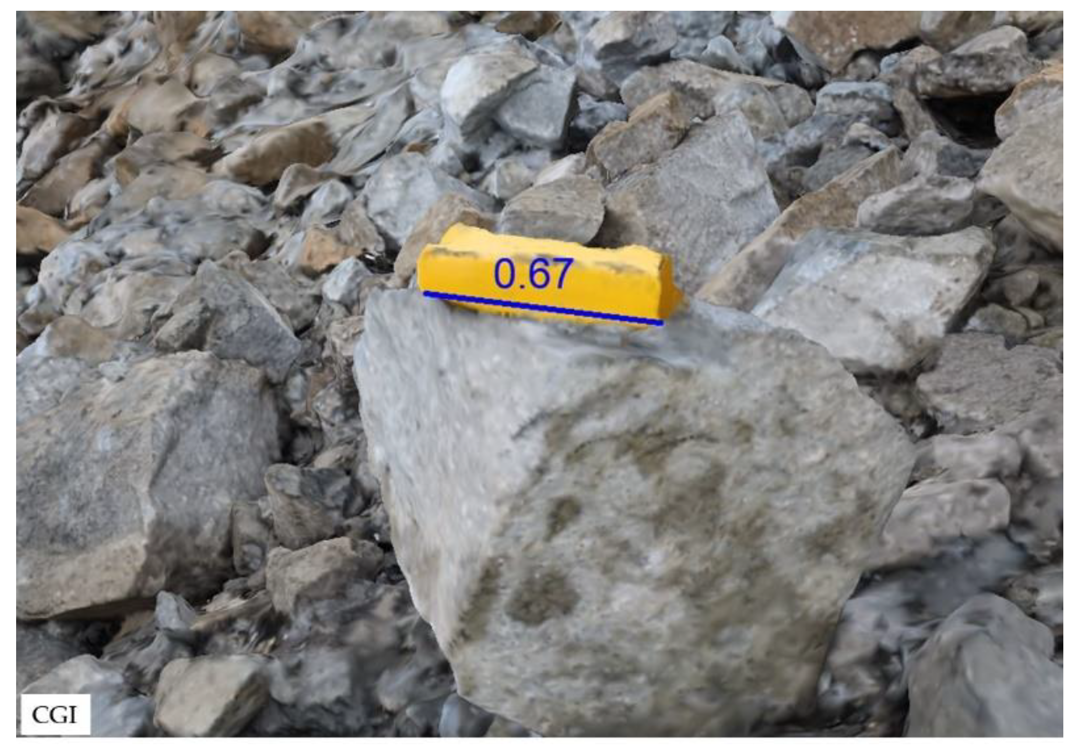
Figure 9.
Close-up of mesh reconstruction, featuring the reference yellow box and the dimension of its longest side as measured.
Figure 9.
Close-up of mesh reconstruction, featuring the reference yellow box and the dimension of its longest side as measured.
Figure 10.
Graph detailing the results of the Mikurahana experiment.
Figure 10.
Graph detailing the results of the Mikurahana experiment.
Figure 11.
Measured fragmentation size distribution in the experimental site. The green bars represent the percentage of each rock size measured by the 3D model, and the gray bars represent that measured by real measurements. The blue line represents the cumulative percentage of rock size measured by the 3D model, and the black dotted line represents that measured by real measurements.
Table 1.
Results of the experiment on the Mikurahana quarry muckpiles.
Table 1.
Results of the experiment on the Mikurahana quarry muckpiles.
Number of
Images | Measured (m) | Real Measurement
(m) | Difference from
Real Measurement (m) | Error (%) |
|---|
| 50 | 0.82 | 0.60 | 0.22 | 36.7 |
| 100 | 0.76 | 0.60 | 0.16 | 26.7 |
| 200 | 0.74 | 0.60 | 0.14 | 23.3 |
| 400 | 0.67 | 0.60 | 0.07 | 11.7 |
| Publisher’s Note: MDPI stays neutral with regard to jurisdictional claims in published maps and institutional affiliations. |
© 2022 by the authors. Licensee MDPI, Basel, Switzerland. This article is an open access article distributed under the terms and conditions of the Creative Commons Attribution (CC BY) license (https://creativecommons.org/licenses/by/4.0/).


 ,
, 


