Preliminary Assessment of Measurement Frequency and Replication Effects on Season-Long Greenhouse Gas Emissions and Global Warming Potential Estimation Consistency Among Various Ecosystems

Abstract

For soil processes that are known to be temporally dynamic, such as soil respiration, methanogenesis, and nitrification–denitrification, it is challenging to capture temporal variations with field-portable greenhouse gas (GHG) analyzers to provide the most accurate estimates of season-long GHG emissions and global warming potentials (GWPs). The objective of this field study was to evaluate the effects of measurement frequency (i.e., weekly, every other week, and every third week), replication (i.e., three, four, or five), and their interaction on the consistency of season-long carbon dioxide (CO₂), methane (CH₄), and nitrous oxide (N₂O) emissions and GWP estimates across multiple ecosystems. Results are based on direct, in-field measurements with a field-portable gas analyzer. Field research was conducted throughout the 2024 growing season in a minimally grazed pasture, tallgrass prairie, soybean under conventional and conservation management practices, and cotton under conservation management in Arkansas, USA. Season-long CO₂ emissions and GWP from the tallgrass prairie were 1.1 times (12%) greater from the weekly and every-other-week (16.9 and 17.0 Mg ha⁻¹, respectively), which did not differ, than the every-third-week (14.2 and 14.2 Mg ha⁻¹, respectively) measurement frequencies. Season-long CH₄ emissions from the minimally grazed pasture and conservation-tilled soybean system were ≥7.5 times greater with four and five replications, which did not differ, than with three replications. Global warming potential in the conservation-tilled soybean (13.9 Mg ha⁻¹) and conservation-tilled cotton (21.1 Mg ha⁻¹) systems were ≥1.1 times (13%) greater with the every-third-week than with the weekly data set. Though this study was somewhat limited due the data sub-setting approach used, even using current, state-of-the-art, field-portable GHG analyzers, an appropriate in-field measurement frequency and number of spatial replications should be considered to reliably quantify whole-field, season-long GHG emissions and GWP estimates.

1. Introduction

Soil is a significant contributor to atmospheric greenhouse gas (GHG) concentrations [1,2], where the documented increase in atmospheric GHG concentrations in the last half century or so [3] is leading to global climate change, particularly via global atmospheric warming, shifting weather patterns, and increasing frequency of extreme weather events [4,5,6].

The processes that produce carbon dioxide (CO₂), methane (CH₄), and nitrous oxide (N₂O) in the soil have been shown to be affected by many factors. Root and microbial respiration produces CO₂, which is generally greater in magnitude from aerobic than anaerobic soil conditions [7,8,9], and is influenced by dynamic environmental characteristics and soil properties, particularly soil moisture and the amount of organic carbon (C) substrate present [i.e., labile organic material and/or the soil C and soil organic matter (SOM) concentration] [10,11,12]. Soil water content fluctuations, in turn, affect the soil oxidation–reduction potential (i.e., Eh), which dictates the transfer of energy (i.e., electrons) between specific soil compounds. Soil Eh is controlled by the soil’s oxygen (O₂) concentration and is strongly correlated with GHG production [13,14,15].

Whereas soil respiration generally dominates under aerobic soil conditions [16,17], when the soil is saturated for an extended period of time, typically requiring several weeks [18], the O₂ concentration decreases to the point where once-aerobic conditions convert to anaerobic conditions, greatly reducing the soil respiration rate. Once the soil becomes anaerobic, reducing conditions can develop, where CO₂ is typically reduced to CH₄ by methanogens via methanogenesis [14,19,20]. However, on a molecule-by-molecule basis, methane’s radiative forcing in the atmosphere is currently recognized as 28 times more powerful than CO₂ [2,21].

Intermediate to the soil conditions that favor CO₂ and CH₄ production, N₂O production generally requires a source of nitrate-nitrogen (N), often as a product of microbial-facilitated SOM decomposition, which is processed by bacteria via denitrification [22,23]. If complete, denitrification produces dinitrogen gas (N₂), which is a major component of the atmosphere, but is not a GHG and thus is not harmful in the atmosphere [24]. However, if incomplete, denitrification can produce N₂O [22,25], which is currently recognized as having an atmospheric radiative forcing 265 times more powerful than CO₂ on a molecule-by-molecule basis [2].

The temporal variability of soil respiration, methanogenesis, and denitrification, all of which are affected by various dynamic environmental conditions and soil physical and chemical properties [26,27], make it challenging to generate accurate estimates of season-long GHG emissions [1,28,29], which, in turn, are critical for accurate and reliable estimates of global warming potential (GWP) from various ecosystems or field treatments. Consequently, designing field studies with statistically sound and valid experimental designs that lead to the generation of high-quality, replicated data representative of field-scale conditions are essential components of GHG emissions and GWP assessments. The appropriate measurement frequency and/or number of spatial replications to include need to be identified and carefully considered to effectively address study objectives. Time commitments for travel to and from research sites, potentially located in geographically widespread locations, and for in-field measurements may require a reduced number of research locations, reduced measurement frequencies, and/or reduced spatial replications. Even when current, state-of-the-art, field-portable, relatively rapid GHG concentration measurement systems are used, the finite time and travel costs available to accomplish the research objectives should play a substantial role in the development of an appropriate experimental design and number of research sites, treatments within a site, measurement frequency, and spatial replications.

In a recent summary of techniques and their advantages and disadvantages, Mumu et al. [26] acknowledged that GHG measurements are technically challenging, often expensive, and laborious, but direct measurements are indispensable for both precision and accuracy of GHG emissions estimates [30]. More specifically, GHG measurements from agricultural soils, which have been identified as globally contributing as much as 25% of all GHG emissions [31], were described as unreliable due to large variability, often associated with choice of sampling or measurement technique [26].

Infrequent (i.e., greater than weekly), temporal measurements may suffice for evaluating relative treatment differences on discrete measurement dates, for soil processes that are known to be temporally dynamic, such as soil respiration, methanogenesis, and nitrification–denitrification. However, it is challenging to capture temporal variations with field-portable, relatively rapid, GHG analyzers to provide the most accurate estimates of true season-long GHG emissions and GWPs [1,28,29,32], particularly when field research sites are geographically separated by long distances that increase travel times [1]. Consequently, compromises may need to be made to reduce the frequency and/or reduce the number of spatial replications of direct, in-field measurements using even state-of-the-art, though field-portable and relatively rapid, GHG analysis systems. However, understanding the sources and magnitudes of uncertainty in GHG emissions estimates is a key component of developing proper measurement protocols, policies, and mitigation strategies and their evaluation [30,32,33,34,35]. Accurate, direct field measurements are also critical for proper up-scaling to whole-field or regional emissions and GWP estimates for most accurate GHG emissions inventorying and budgets [30] and are equally critical for proper GHG model calibration and validation.

The objective of this field study was to evaluate the effects of measurement frequency, replication per ecosystem, and their interaction on season-long GHG emissions and GWP estimates, based on direct, in-field measurements, separately in five diverse ecosystems at different sites using measurements conducted throughout the 2024 growing season in Arkansas, USA. For the current study, it was hypothesized that, in general, season-long GHG emissions and GWP results from less frequent measurements than weekly and/or from fewer than four spatial replications would result in greater uncertainty (i.e., greater variability) than from the most robust data set collected, represented by weekly measurements with four or more spatial replications, due to data reduction. It was also hypothesized that, due to more stable environmental conditions (i.e., soil moisture variations in response to rainfall only), the grassland ecosystems would have fewer differences in season-long GHG emissions and GWP results when measurement frequency and/or replications were reduced than the agroecosystems, as rainfall plus the furrow-irrigated water management in the agroecosystems would create more soil moisture fluctuations in the warmer and wetter climate region where the agroecosystems were located.

The novelty of this field study lies in the multi-ecosystem design that extends beyond previous single-site studies and volume of GHG flux data collected consistently across multiple ecosystems throughout the same summer growing season as the basis to calculate season-long GHG emissions and GWP estimates. In addition, this study addressed both spatial and temporal resolution effects on GHG consistency, whereas most other studies only focus on one of the two aspects of emissions variability, and addressed effects on the simultaneous measurement of CO₂, CH₄, and N₂O as a group, rather than focusing on single-gas responses.

2. Materials and Methods

2.1. Site Descriptions

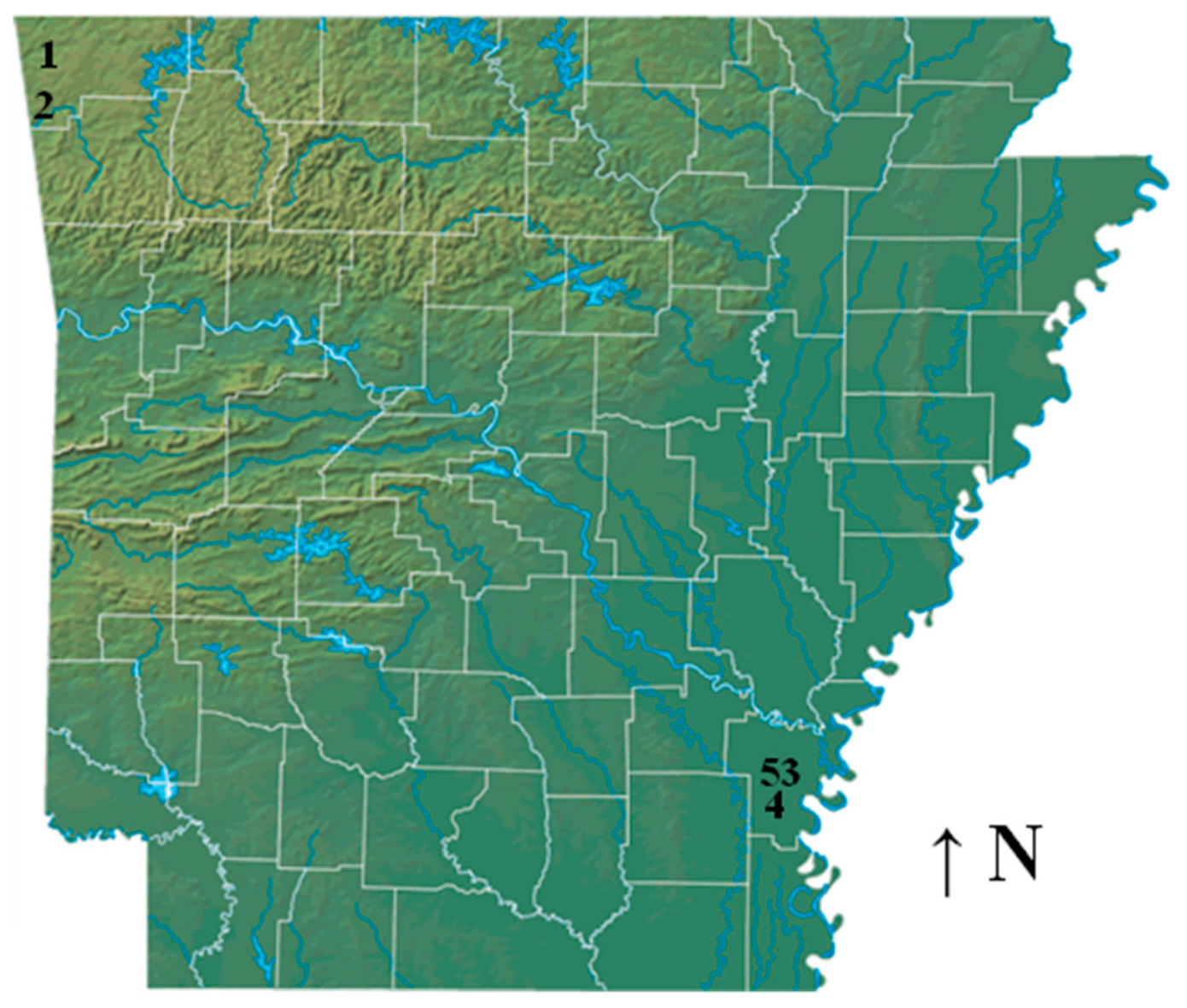
Field research was conducted over the course of the 2024 growing season in five different ecosystems throughout Arkansas (Figure 1;

Table 1. Summary of ecosystems and their characteristics for which season-long greenhouse gas fluxes were measured across Arkansas throughout the 2024 growing season.

Ecosystem	Location	Vegetation Type/Crop	Management Practices/Important Characteristics	Soil Taxonomic Description	Measurement Date Range	Measurement Duration (Days)
Grassland	Northwest Arkansas	Pastureland	Minimally grazed, non- irrigated, udic soil moisture regime	Fine-silty, mixed, active, mesic Typic Paleudalfs	30 May to 30 August	93
		Tallgrass prairie	Native prairie, never plowed, prairie mounds present, udic soil moisture regime	Fine-silty, mixed, active, thermic Oxyaquic Fragiudalfs	16 May to 13 September	121
Agroecosystem	Southeast Arkansas	Soybean	Conventional tillage, furrow-irrigated, aquic soil moisture regime	Fine, smectitic, thermic Typic Albaqualf	7 May to 20 August	106
		Soybean	Reduced/conservation tillage, furrow-irrigated, aquic soil moisture regime	Fine-silty, mixed, active, thermic Aeric Epiaqualfs	8 May to 20 August	105
		Cotton	Conservation tillage, furrow-irrigated, aquic soil moisture regime	Fine-silty, mixed, active, thermic Aeric Epiaqualfs	8 May to 9 September	125

). Two grassland ecosystems in northwest Arkansas (i.e., a minimally grazed pasture [36] and a native tallgrass prairie [37]) were investigated, while three agroecosystems from southeast Arkansas (i.e., a conventionally tilled, furrow-irrigated soybean system without cover crops, representing a conventional production system [38]; a reduced tillage, furrow-irrigated soybean system with cover crops, representing a conservation production system [39]; and a conservation-tilled, furrow-irrigated cotton system without cover crops, representing a conservation production system [40]) were investigated (Figure 1; Table 1). In the agroecosystems, tillage depths were generally 5 to 10 cm, irrigation frequency was generally once per week, and cereal rye (Secale cereale) was the cover crop if present. The grazed pasture system received 60 kg N ha⁻¹ as urea in August 2024 [26]. The conventional soybean system had 56 kg ha⁻¹ of ammonium sulfate applied on 1 June 2024 [38]. The conservation soybean system had 11 kg ha⁻¹ of urea ammonium nitrate (UAN) applied after planting and 56 kg ha⁻¹ of ammonium sulfate were applied on 1 June 2024 [39]. The cotton system had 112 kg ha⁻¹ of diammonium phosphate applied on 10 June and 87 L of UAN applied on 25 June 2024 [40]. All five ecosystems had soils with silt-loam surface textures (

Table 2. Summary of initial soil property means (n = 4 for the cotton system, n = 5 for the other four ecosystems) and their standard errors (SEs) from the beginning of the 2024 growing season in the top 10 cm for the two grasslands and in the top 15 cm in the three agroecosystems.

Ecosystem	Sand (g g−1)	Silt (g g−1)	Clay (g g−1)	BD † (g cm−3)	pH	SOM † (Mg ha−1)	TN † (Mg ha−1)	TC † (Mg ha−1)
Minimally grazed pastureland	0.51 (0.01)	0.43 (<0.01)	0.06 (0.01)	1.29 (0.02)	5.3 (0.05)	45.0 (1.2)	2.4 (0.1)	24.7 (0.7)
Tallgrass prairie	0.28 (<0.01)	0.67 (<0.01)	0.05 (<0.01)	0.91 (0.02)	4.9 (0.05)	49.4 (1.6)	2.4 (0.1)	28.6 (1.0)
Conventionally tilled soybean	0.22 (<0.01)	0.67 (<0.01)	0.10 (<0.01)	1.29 (0.1)	7.48 (0.1)	41.3 (1.1)	1.8 (0.1)	21.1 (1.0)
Conservation-tilled soybean	0.28 (<0.01)	0.65 (<0.01)	0.07 (<0.01)	1.18 (0.03)	6.8 (0.03)	34.3 (0.9)	1.5 (<0.1)	17.9 (0.2)
Conservation-tilled cotton	0.15 (<0.01)	0.79 (<0.01)	0.06 (<0.01)	1.27 (<0.1)	6.8 (<0.1)	45.2 (2.9)	2.3 (0.2)	25.9 (2.3)

^† BD, bulk density; SOM, soil organic matter; TN, total nitrogen; TC, total carbon.

). The two northwest Arkansas locations were mapped in a udic, while the three southeast Arkansas locations were mapped in an aquic soil moisture regime, but all soils evaluated were mapped as Alfisols with argillic sub-surface horizons. Greenhouse gas concentration measurements within the ecosystems took place over different date ranges, at different times of the day, and different durations among ecosystems, but generally occurred between mid-May and mid-September 2024, representing between 93 and 125 days of the major portion of each ecosystem’s summer growing season (Table 1). However, within each individual ecosystem, GHG measurements occurred during the same temporal window and followed a constant protocol for the whole growing season.

Table 3. Summary of mean monthly and growing season air temperature and rainfall for 2024 and 30-year (i.e., 1991–2020) average monthly and growing season air temperature and rainfall for the pastureland and tallgrass prairie ecosystems in northwest Arkansas and agroecosystems in southeast Arkansas.

Ecosystem/ Climate Metric	April	May	June	July	August	September	Growing Season
Pastureland †
Air temperature (°C)	16.0	21.0	25.4	26.3	26.9	-	23.1
30-year mean (°C)	14.6	19.1	23.8	26.4	25.9	-	22.0
Rainfall (mm)	105	170	59	83	77	-	494
30-year mean (mm)	126	150	109	106	85	-	577
Tallgrass prairie ‡
Air temperature (°C)	-	21.1	25.3	26.4	26.7	22.5	24.4
30-year mean (°C)	-	20.3	24.8	27.2	26.7	22.4	24.3
Rainfall (mm)	-	190	58	74	57	1	380
30-year mean (mm)	-	161	115	106	91	110	583
Agroecosystems #
Air temperature (°C)	18.4	23.5	26.9	27.5	28.3	24.3	24.9
30-year mean (°C)	18.1	22.6	26.4	27.7	27.2	24.0	24.3
Rainfall (mm)	95	193	63	96	48	25	520
30-year mean (mm)	141	125	84	86	74	72	582

^† Monthly air temperature and rainfall from NOAA-NESDI [41,42] and 30-year averages from NOAA-NCEI [43]. ^‡ Monthly air temperature and rainfall from NOAA-NESDI [41,42] and 30-year averages from NOAA-NCEI [43]. ^# Monthly air temperature and rainfall from SRCC [44] and 30-year averages from NOAA-NCEI [43].

summarizes the mean monthly and growing season air temperature and rainfall for 2024 and the 30-year (i.e., 1991–2020) average monthly and growing season air temperature and rainfall for the three locations that include all five ecosystems included in this study. The pastureland and tallgrass prairie in northwest Arkansas had similar 2024 growing-season mean air temperatures, but substantially lower growing-season rainfall compared to the 30-year averages (Table 3). The agroecosystems in southeast Arkansas also had similar 2024 growing-season mean air temperatures and lower growing-season rainfall compared to the 30-year averages (Table 3), but all three agroecosystems were furrow-irrigated to supply adequate moisture.

2.2. Treatments and Experimental Design

Measurement frequency and number of replications were the two formal factors evaluated in this study, where data sets for both factors were derived from the same original data set consisting of weekly GHG measurements with four or five replications, which was considered the most robustly gathered data set. Weekly measurements were the most practically achievable frequency given that three of the five study locations were located ~370 km one-way away from the home campus. Five replications were based on a power analysis (1 − β > 0.90) from several preliminary GHG measurements conducted prior to the first formal measurement date included in the data sets, thus the preliminary measurements were not included in the formal data sets analyzed in this study. The measurement frequencies evaluated included gas-flux data from measurements conducted weekly, every other week, and every third week. As weekly measurements were the original data set generated, to create the every-other-week and every-third-week data sets, the first measurement date was always retained, then subsequent data from only every other week and only every third week were retained from the original weekly data set, while all other data were deleted.

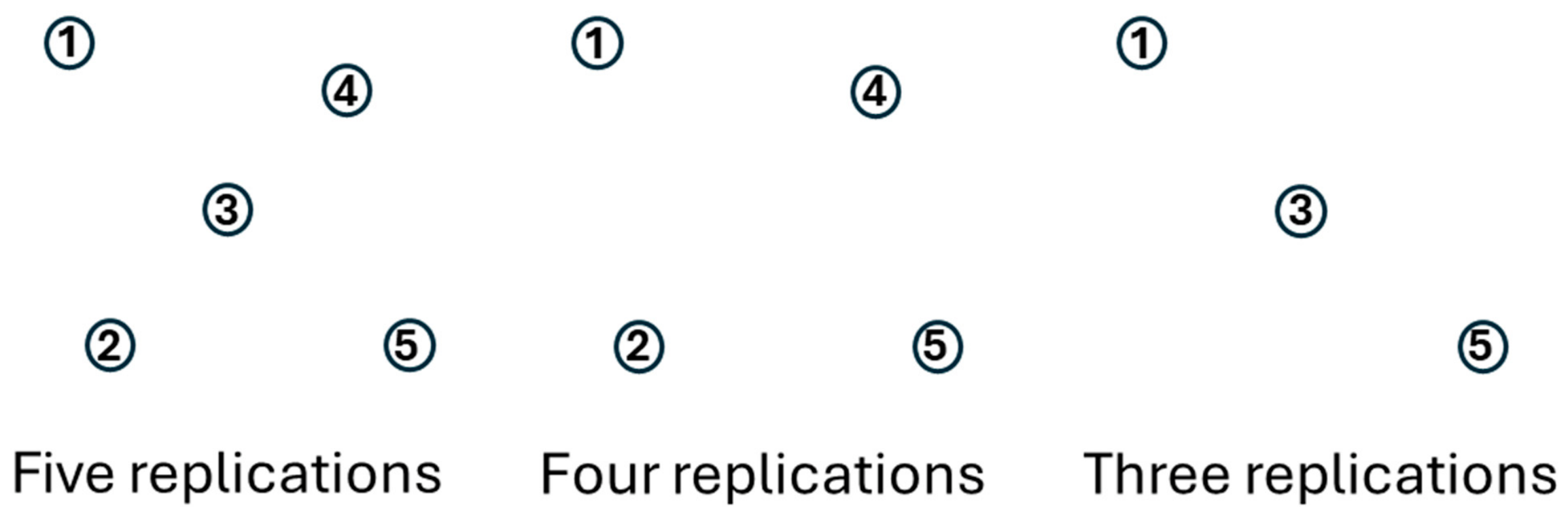
The number of spatial replications evaluated were three, four, and five for all ecosystems, except the cotton system, for which only three and four replications were evaluated. For four of the five ecosystems, excluding the cotton system, the same replications were systematically deleted from the original five-replication data set for each ecosystem, thus not all possible combinations of deleted replications were evaluated, but all four ecosystems had the same replicate data deleted to create the three- and four-replication data sets (Figure 2). Eliminating the center replicate was justified to create the four-replicate data set (Figure 2), as the center replicate likely represented intermediate GHG fluxes among the four remaining replicates. Eliminating two different replicates to create the three-replication data set left replicates in the same horizontal plane, resulting in a 3-point transect, which would be a logical arrangement choice for only three replications (Figure 2). It is possible that the results may differ had a different combination of spatial replicates been removed. However, assessing all combinations of possible replicate removals was beyond the scope of this study, as the approach used in this study represented reasonably logical choices for designing a similar field experiment if resources or time required limiting the number of measurement replications. Other possible replicate combinations would result in an impractical arrangement of replicates.

For the cotton system, only four replications were measured originally, thus, to create the three-replication data set, the fourth replication was simply deleted. Though replications within each ecosystem were established in a spatially discrete arrangement, a completely random experimental design was assumed for data analyses for all ecosystems. Due to differences in growing season lengths and ecosystem characteristics (Table 1), the effects of measurement frequency, replication, and their interaction were evaluated separately by ecosystem, thus no formal comparisons among ecosystems were made.

2.3. Gas Concentration Measurements

At each location, five base collars were installed in a consistent, spatially discrete arrangement. Base collars consisted of thick-walled, 20 cm diameter, 11.5 cm tall, polyvinyl chloride (PVC), beveled to the outside at the bottom to facilitate installation, which were manually tapped into the soil to a depth of ~9 cm using a rubber mallet and a wooden board and leveled with a bubble level. Greenhouse gas measurements occurred weekly throughout the growing season at each of the five locations (Table 1). Measurements in the three agroecosystems were conducted between 0700 and 1000 h (i.e., 7 and 10 am) or between 1700 and 2000 h (i.e., 5 and 8 pm), which corresponded to when the average daily air temperature occurred for when GHG measurements are recommended [45], while measurements in the two grasslands were conducted between 1000 and 1400 h (i.e., 10 am and 2 pm) due to travel logistics.

A field-portable, Li-Cor trace gas measurement system (Li-Cor Inc., Lincoln, NE, USA) was used for all in-field GHG measurements, which consisted of a smart chamber (LI-8200-01S), a combined CO₂ and CH₄ analyzer (LI-7810), and a N₂O analyzer (LI-7820). The chamber has a volume of ~5158 cm³. The analyzers have detection ranges of 0–100 ppm for CH₄ and N₂O and 0–100,000 ppm for CO₂ [46]. For each base collar measurement, the chamber was placed atop the uncovered base collar in the open position. Via a wi-fi-connected smart device (i.e., a phone or tablet), the measurement sequence was activated remotely, which closed the chamber to create an air-tight, closed-loop system. The measurement sequence, which circulated the chamber’s headspace air through the analyzers, lasted 320 s. Optical feedback-cavity enhanced absorption spectroscopy (OF-CEAS) [46] quantified the gas concentrations every 1 s the chamber was closed. Once a single measurement was completed, the smart chamber opened and air was force-circulated through the tubing and analyzers for 45 s to flush the system. Base collars remained in the same position for the entire growing season and experienced the same environmental conditions as outside the base collars (i.e., shade, soil water content, relative humidity, and physical, chemical, and biological properties), as only 9 cm of the base collar was above the soil surface.

After all measurements at a location ceased, data were downloaded from the gas analyzers and smart chamber and imported into Li-Cor’s Soil Flux Pro software (version 5.3.1) before leaving the field location to check for data quality. In Soil Flux Pro, the first 45 s of each set of measured gas concentrations were excluded from subsequent calculations as a dead-band period of instability with the measured gas concentrations early in the measurement sequence. Thus, the actual sampling period for data analyses was 75 and 275 s for CO₂/CH₄ and N₂O, respectively, so that a linear regression model could be fit to the concentration-over-time data to determine each gas’ dry flux, which was represented by the slope of the linear regression equation and was reported as the change in gas concentration per unit area per unit time (i.e., μmol m⁻² s⁻¹). Following procedures outlined by Parkin and Venterea [45], if the original regression slope was negative, the negative flux was reassigned to a value of 1.0 × 10⁻⁶, such that all fluxes were positive for statistical analysis purposes. Numerous recent studies [47,48] have considered only positive gas fluxes, as the true mechanism responsible for a negative measured flux is not well-understood yet, thus results reflect soil effluxes rather than net ecosystem exchange.

Over the course of the 2024 growing, there were a total of 14, 18, 16, 16, and 19 weekly measurement dates in the minimally grazed pasture, tallgrass prairie, conventionally tilled soybean, conservation-tilled soybean, and conservation-tilled cotton systems, respectively. Greenhouse gas data for the grazed pasture and conventionally tilled soybean system were extracted from Buchanan et al. [36] and Gwaltney et al. [38], respectively.

2.4. Soil Sample Collection, Processing, and Analyses

To characterize initial near-surface soil properties, after base collars were first installed in late April to mid-May 2024, soil samples were collected with a 4.8 cm diameter, stainless-steel core chamber and slide hammer from within 0.3 m of each base collar from the top 10 cm in the two grassland ecosystems and from the top 15 cm in the three agroecosystems. Different sample depths reflected established recommendations for assessing in soil fertility requirements in the different ecosystems. Samples were collected from the top and middle of the raised beds in the three agroecosystems.

Samples were oven-dried in a forced-draft oven at 70 °C for at least 48 h, weighed for bulk density determination, ground, and sieved through a 2 mm mesh screen for select soil physical and chemical property assessments. Sand, silt, and clay concentrations were measured using a modified 12 h hydrometer method [49]. Soil pH was measured potentiometrically with an electrode in a 1:2 soil mass:water volume suspension [50]. High-temperature combustion was used to measure total C (TC) and total N (TN) concentrations on a VarioMax CN analyzer (Elementar Americas Inc., Mt. Laurel, NJ, USA) [51,52]. Since no effervescence occurred when soil was treated with dilute hydrochloric acid, all measured TC was assumed to be organic [51]. Weight-loss-on-ignition was used to measure SOM concentration after 2 h of combustion at 360 °C [53]. On a collar-by-collar basis, measured SOM, TC, and TN concentrations (%) were converted to contents (Mg ha⁻¹) by multiplying by the measured bulk density and multiplying by the appropriate sample depth (i.e., 10 or 15 cm). Soil property data were extracted from Buchanan et al. [36] for the grazed pasture system, Dockery [37] for the native prairie, Gwaltney et al. [38] for the conventionally tilled soybean system, Brye [39] for the conservation managed soybean system, and Seuferling et al. [40] for the conventionally managed cotton system. Initial soil property means for all five systems are summarized in Table 2.

2.5. Season-Long Emissions and Global Warming Potential Determinations

Following recent procedures, on a collar-by-collar basis, each original hourly gas flux was converted to a daily flux using the appropriate air temperature, atmospheric pressure, and chamber volume. Daily gas fluxes were then linearly interpolated between consecutive measurement dates, which were subsequently summed to estimate season-long emissions following procedures of numerous recent studies [48,54].

On a collar-to-collar basis, three-gas GWP was calculated as the sum of CO₂ equivalents (eq) for CO₂, CH₄, and N₂O, with 100-year conversion factors of 1, 28, and 265 for CO₂, CH₄, and N₂O, respectively [2]. Due to CO₂’s substantially larger emissions magnitudes compared to CH₄ and N₂O in terms of molar mass, a two-gas, reduced GWP (GWP*) was also calculated in the same manner as GWP on a collar-to-collar basis, but with only CH₄ and N₂O included and CO₂ excluded, as the inclusion of CO₂ in the GWP calculation can potentially mask treatment differences [47,48].

Original hourly gas-flux data were previously reported, where temporal trends and field treatments were formally evaluated [36,37,38,39,40]. Consequently, descriptions of the original hourly flux data and temporal and field treatment effects were not repeated in the current study, rather the 2024 season-long GHG emissions were evaluated in a manner that had not previously been conducted. Furthermore, being summed across all weekly measurement dates, thus representing a cumulative response for a 3- to 4-month-long period rather than discrete, 5 min responses from week to week, season-long GHG emissions convey substantially greater climate-change implications than GHG fluxes. In addition to being the foundation of GWP estimations, sustainability metrics and climate-change policies associated with various crops and cropping systems are based on longer-term, cumulative emissions rather than short-term fluxes.

2.6. Statistical Analyses

Due to logistical and practical limitations that precluded fully independent treatments associated with a study location, the different measurement frequencies and replication levels were created as sub-sets of the original complete data sets at each location. Thus, based on prior observations from northwest Arkansas, it was reasonably assumed that the within-field variability would have been similar to the between-field variability had multiple fields been able to be included in this study for each study location [55]. Therefore, based on a completely random design, a two-factor analysis of variance (ANOVA) was conducted using the PROC GLIMMIX procedure in SAS (version 9.4, SAS Institute Inc., Cary, NC, USA) to evaluate the effects of measurement frequency (i.e., weekly, every other week, and every third week), replications (i.e., three, four, or five), and their interaction on season-long GHG (i.e., CO₂, CH₄, and N₂O) emissions and GWP and GWP* estimates separately among five ecosystems (i.e., minimally grazed pastureland, tallgrass prairie, soybean under conventional and conservation management practices, and cotton under conventional management). The five ecosystems were not formally compared to one another and analyzed separately due to the variations in environmental conditions (i.e., air temperature and rainfall) experienced, differences in treatments evaluated, and differences in growing season durations among the ecosystems. Consequently, consistencies in results across the five ecosystems were the intended focus of this study. Measurement frequency and replication were the evaluated fixed effects, while the random effect was the three, four, of five actual observations that made up the replication fixed effect. All response variables were analyzed with a gamma distribution. Since the closest distance between any two GHG base collars was no less than 3 m, all gas-flux data were assumed independent and treated as separate observations for all statistical analyses. Sample independence at a similar distance among replicate observations has been formally evaluated in numerous locations throughout Arkansas and specifically in soils in eastern Arkansas [56,57,58]. Though an increased rate of false positive responses may occur, due to the combination of large, expected variability among spatial replications from prior direct field measurements and low number of observations [59], significance was judged at p ≤ 0.1 for all response variables. Means were separated by least significant difference when appropriate.

Though most often applied when treatment factors are material effects, the ANOVA approach used in this study evaluated non-material effects (i.e., measurement frequency and replication), which allowed for the main effects to be evaluated separately and their interaction to be evaluated. In the current study, the interaction effect tested whether any measurement frequency effect on GHG emissions consistency differed among replications used and vice versa, which was a unique and novel aspect of this study. Furthermore, the ability of ANOVA to handle unbalanced data sets made the current statistical approach robust, replicable, and reliable. However, since the data sets evaluated were a sub-set of an originally collected, complete data set, the data sub-sets are not truly independent and may have affected the variance components. Consequently, results from this study should be considered preliminary, with additional observations and analyses conducted before results are confirmed.

In addition, to address uncertainty, standard error of the mean across treatment combinations and the effect size (η²) across fixed factors were used to assess the level of uncertainty and the practical significance within the ANOVA analysis for each response variable in the various ecosystems. The η² was calculated as the ratio between the sum of square (SS) of a specific fixed effect and the total SS of the model.

3. Results and Discussion

3.1. Season-Long Emissions

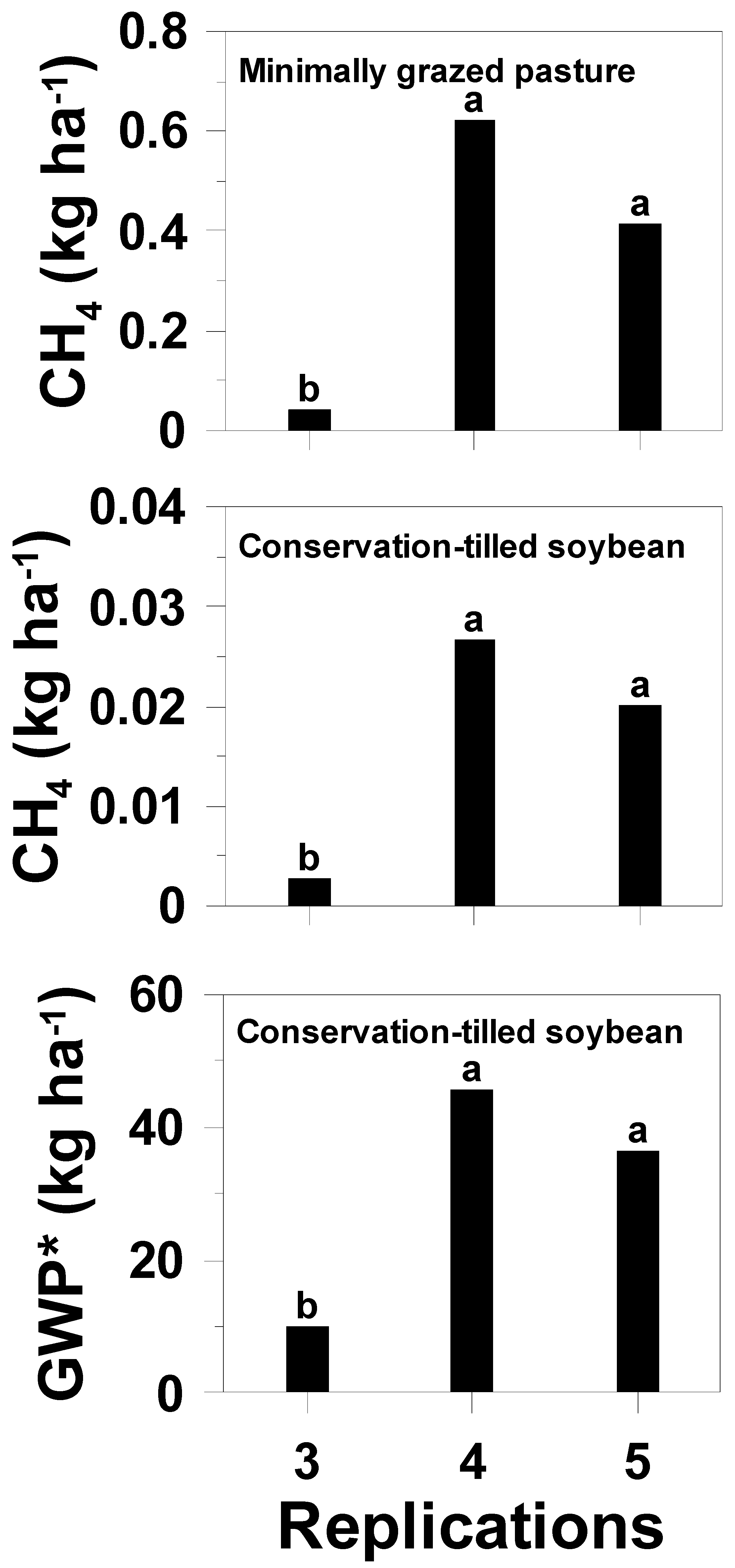
Season-long emissions for at least one GHG were affected (p ≤ 0.1) by measurement frequency or replication in each ecosystem, except for the conventionally tilled soybean system, for which season-long emissions for all three GHGs were unaffected (p > 0.1) by measurement frequency and replication (

Table 4. Analysis of variance summary for the effects of measurement frequency, replication, and their interaction on season-long carbon dioxide (CO₂), methane (CH4), nitrous oxide (N₂O), three-gas global warming potential (GWP), and reduced GWP (GWP*) excluding CO₂ within several different ecosystems across Arkansas during 2024.

Ecosystem	Response Variable	Frequency	Replication	Frequency × Replication
		________________________ p ________________________
Minimally grazed pastureland	CO2	0.43	0.18	0.99
	CH4	0.64	<0.01	0.73
	N2O	0.94	0.31	1.0
	GWP	0.46	0.18	0.99
	GWP*	0.95	0.27	1.0
Tallgrass prairie	CO2	<0.01 †	0.47	1.0
	CH4	- ‡	-	-
	N2O	0.75	0.79	1.0
	GWP	<0.01	0.49	1.0
	GWP*	0.75	0.79	1.0
Conventionally tilled soybean	CO2	0.62	0.65	1.0
	CH4	0.96	0.97	1.0
	N2O	0.20	0.55	0.99
	GWP	0.64	0.68	1.0
	GWP*	0.78	0.91	1.0
Conservation-tilled soybean	CO2	0.05	0.58	1.0
	CH4	0.39	<0.01	0.95
	N2O	0.42	0.14	0.70
	GWP	0.05	0.58	1.0
	GWP*	0.50	0.06	0.75
Conservation-tilled cotton	CO2	<0.01	0.22	0.75
	CH4	-	-	-
	N2O	0.36	0.42	1.0
	GWP	<0.01	0.20	0.75
	GWP*	0.37	0.42	1.0

^† Bolded values are significant at p ≤ 0.1. ^‡ Cells with dashes (-) did not have sufficient data to complete the formal statistical analyses.

). From the minimally managed grazed pasture, season-long CO₂, CH₄, and N₂O emissions were unaffected (p > 0.1) by measurement frequency and season-long CO₂ and N₂O emissions were unaffected (p > 0.1) by replication (Table 4). In contrast, season-long CH₄ emissions were at least 10 times greater with four and five replications, which did not differ, than with three replications in the minimally grazed pasture (Figure 1).

Similar to the minimally grazed pasture, season-long N₂O emissions were unaffected (p > 0.1) by measurement frequency and season-long CO₂ and N₂O emissions were unaffected (p > 0.1) by replication in the tallgrass prairie (Table 4). There were insufficient data (i.e., no significantly positive measured fluxes for any replicate on any of the 15 measurement dates) to formally test season-long CH₄ emissions in the tallgrass prairie due to the lack of extended periods of soil saturation. However, season-long CO₂ emissions from the tallgrass prairie were at least 1.1 times (12%) greater from the weekly and every-other-week measurement frequencies, which did not differ, than the every-third-week measurement frequencies (

Table 5. Summary of the effect of measurement frequency, averaged across replications, on season-long carbon dioxide (CO₂), methane (CH₄), nitrous oxide (N₂O), three-gas global warming potential (GWP), and reduced GWP (GWP*) excluding CO₂ within several different ecosystems across Arkansas during 2024.

Ecosystem	Measurement Frequency	Season-Long Emissions			GWP (Mg ha−1)	GWP* (kg ha−1)
		CO2 (Mg ha−1)	CH4 (kg ha−1)	N2O (kg ha−1)
Minimally grazed pastureland	Every week	17.8 a	0.16 a	0.37 a	17.9 a	102.3 a
	Every other week	17.9 a	0.25 a	0.43 a	18.0 a	118.2 a
	Every third week	18.9 a	0.27 a	0.41 a	19.1 a	112.4 a
Tallgrass prairie	Every week	17.6 a †	-	0.41 a	17.7 a	107.5 a
	Every other week	16.1 a	-	0.46 a	16.3 a	122.0 a
	Every third week	14.2 b	-	0.36 a	14.3 b	95.9 a
Conventionally tilled soybean	Every week	17.3 a	12.5 a	0.49 a	17.8 a	479.8 a
	Every other week	17.2 a	14.2 a	0.80 a	17. a	612.2 a
	Every third week	18.2 a	17.0 a	0.53 a	18.8 a	620.9 a
Conservation-tilled soybean	Every week	12.3 b	0.008 a	0.10 a	12.3 b	21.3 a
	Every other week	12.8 ab	0.009 a	0.18 a	12.9 ab	39.0 a
	Every third week	13.9 a	0.019 a	0.09 a	13.9 a	20.3 a
Conservation-tilled cotton	Every week	17.9 b	-	0.56 a	18.0 b	147.9 a
	Every other week	20.7 a	-	0.62 a	20.9 a	164.8 a
	Every third week	20.9 a	-	0.83 a	21.1 a	220.9 a

^† Means in a column within an ecosystem with different lower-case letters are different at p < 0.1.

).

Similar to the minimally grazed pasture, but unlike the tallgrass prairie, season-long CO₂, CH₄, and N₂O emissions were similar among the weekly, every-other-week, and every-third-week measurement frequencies and were similar among three, four, or five replications from the conventionally tilled soybean system in southeast Arkansas (Table 4 and Table 5). The lack of treatment effects on GHG emissions in the conventionally tilled soybean system suggests that both the temporal and spatial variability were minimal in the conventionally tilled soybean system. Similar to the conventionally tilled soybean system, season-long CH₄ and N₂O emissions were unaffected (p > 0.1) by measurement frequency and season-long CO₂ and N₂O emissions were unaffected (p > 0.1) by replication from the conservation-tilled soybean system (Table 4). However, in contrast to the conventionally tilled soybean system, season-long CO₂ emissions from the conservation-tilled soybean system were 1.1 times (13%) greater for the every-third-week than weekly measurement frequency, while season-long CO₂ emissions for the every-other-week measurement frequency were intermediate and similar to that from both the every-third-week and weekly measurement frequencies (Table 4 and Table 5). Similar to CH₄ from the minimally grazed pasture, season-long CH₄ emissions from the conservation-tilled soybean system were at least 7.5 times greater with four and five replications, which did not differ, than with three replications (Figure 1).

Similar to the conservation-tilled soybean system, season-long N₂O emissions were unaffected (p > 0.1) by measurement frequency and replication, while season-long CO₂ emissions were 1.2 times (16%) greater for the every-other-week and every-third-week, which did not differ, than the weekly measurement frequency from the conservation-tilled cotton system (Table 4). Like the tallgrass prairie, there were insufficient data (i.e., only one of four replications of the unamended control treatment had one or more significantly positive measured fluxes for the whole growing season) to formally test season-long CH₄ emissions from the conventionally tilled cotton system due to the lack of an extended period of soil saturation (Table 4). However, for both the tallgrass prairie and conservation-tilled cotton systems, since season-long CH₄ emissions were zero, season-long CH₄ emissions were not included in the GWP estimates. Season-long N₂O emissions were unaffected (p > 0.1) by measurement frequency and replication in each of the five ecosystems evaluated (Table 4).

Compared to the weekly measurement frequency with five spatial replications, which was the most robust data set collected among all five ecosystems, averaged across number of replications, season-long CH₄ and N₂O emissions for the every-other-week and every-third-week data sets for each of the five ecosystems evaluated did not differ from the weekly data set (Table 4 and Table 5). Thus, despite CH₄ and N₂O having greater impacts, on a molecule-by-molecule basis, on atmospheric heat absorption than CO₂, it appears that a reduction in measurement frequency from weekly may be a reasonable time and/or resource compromise to make, if necessary. Furthermore, this recommendation is particularly justified considering the three to more than five orders of magnitude lower CH₄ and N₂O emissions compared to the magnitude of season-long CO₂ emissions (Table 5).

Similar to CH₄ and N₂O, season-long CO₂ emissions for the minimally grazed pasture and conventionally tilled soybean systems from the every-other-week and every-third-week data sets did not differ from the weekly data set (Table 5). However, in contrast to CH₄ and N₂O, season-long CO₂ emissions were significantly lower from the every-third-week data set in the tallgrass prairie, greater from the every-third-week data set in the conservation-tilled soybean, and greater from both the every-other-week and every-third-week data sets in the conservation-tilled cotton system (Table 5). Consequently, despite weekly measurements requiring greater time and resource commitment to achieve, reducing the measurement frequency from weekly significantly over- or under-estimated season-long CO₂ emissions in one grassland and two agroecosystems among the five total ecosystems evaluated in this study. With the orders of magnitude greater season-long CO₂ compared to CH₄ and N₂O emissions, which accounted for >97% of all GWP estimates across all five ecosystems and measurement frequencies (Table 5), over- or under-estimating season-long CO₂ emissions could introduce substantial numeric inaccuracies for GWP estimates.

Regarding N₂O specifically in the absence of simultaneous CO₂ and CH₄ measurements, Lammirato et al. [35] reported that the largest variation in the accuracy of N₂O emissions estimates occurred when the measuring frequency was reduced from daily or sub-daily or increased to every second or third day. Thus, considering N₂O emissions estimates alone, weekly measurements, as were used as the most frequent GHG measurement frequency in the current study, may have already been too low of a measurement frequency if trying to assess effects of only N₂O emissions estimates. However, the current study purposefully examined effects on simultaneous CO₂, CH₄, and N₂O measurements as a group, rather than examine effects on single-gas responses. Furthermore, Parkin and Venterea [45] indicated that weekly sampling to measure GHGs represents an ideal frequency during the growing season in an agricultural setting.

Similar to measurement frequency, compared to weekly measurements with five spatial replications, averaged across measurement frequency, season-long CO₂ and N₂O emissions from the three-replication data set for each of the five ecosystems evaluated did not differ from the four- or five-replication data set (Table 4). Similarly, season-long CH₄ emissions from the three-replication data set for the conventionally tilled soybean system did not differ from the four- or five-replication data set (Table 4 and Table 5). However, the three-replication data set significantly under-estimated season-long CH₄ emissions for the minimally grazed pasture and conservation-tilled soybean systems, for which the four- and five-replication data sets were similar (Table 4; Figure 3).

It appears that reducing the number of spatial replications, at least for season-long CH₄ emissions estimations in one grassland and one agroecosystem among the five total ecosystems evaluated in this study, created compromised results. Consequently, though reducing the number of spatial replications out of necessity may be sufficient for assessing relative differences among ecosystems or field treatments, it may not be advisable to reduce the number of spatial replications to only three for all measurement dates when planning for season-long GHG emissions estimates. However, in this study, positive CH₄ concentrations (i.e., measured CH₄ efflux) were sporadic across the growing season in all five ecosystems evaluated. Soil water contents rarely achieved the requisite level and duration to stimulate methanogenesis, resulting in many weeks where CH₄ fluxes were either zero or negative, in which the negative fluxes were reassigned to a small positive value. Thus, creating a resulting data set used in the current study with little variation, but with a few spatially and temporally random, but highly influential fluxes likely skewed statistical analyses some. In a climatically wetter growing season and/or in an environment where soil water contents were at or near saturation for extended durations (i.e., in a flooded rice field), CH₄ emissions may be more stable in time and space and less sensitive to reduced replication. Despite the semi-frequent furrow-irrigation management among all three agroecosystems, the magnitude of N₂O emissions was relatively small and was consistently unaffected by measurement frequency and replication (Table 5), which was somewhat contrary to what was expected.

Few studies have formally evaluated the potential effects of the number of spatial replications on response variables, particularly GHG emissions. However, using a suite of 20 near-surface soil properties, the degree of potential observation (i.e., replication) reduction that could maintain the ability to identify significant differences was evaluated at 15-m intervals along a 60-m line transect in multiple prairie ecosystems with silt-loam soils in the Ozark Highlands of northwest Arkansas and in the Grand Prairie region of east-central Arkansas [58]. The ability to identify significant treatment differences was generally maintained when reducing the number of spatially independent observations from five to four [58]. However, three or fewer observations resulted in a non-significant treatment effect for more than 25% of the soil properties, including SOM, total C, and total N, when the original five-observation data set identified a significant treatment effect [48]. Thus, consistent with results of the current study, three spatially independent replications appear to be marginal to achieve accurate results and may result in compromised interpretations and inferences.

3.2. Global Warming Potentials

Similar to season-long GHG emissions, at least one of the two GWP estimates were affected (p ≤ 0.1) by measurement frequency or replication in three of five ecosystems, except for the conventionally tilled soybean system and the minimally grazed pasture, for which both GWP estimates were unaffected (p > 0.1) by measurement frequency and replication (Table 4). In the tallgrass prairie, two-gas GWP* was unaffected (p > 0.1) by measurement frequency and both GWP estimates were unaffected (p > 0.1) by replication (Table 4). However, in the tallgrass prairie, three-gas GWP was at least 1.1 times (12%) greater with the weekly and every-other-week data sets, which did not differ, than with the every-third-week data set (Table 5).

Similar to the tallgrass prairie, GWP* quantification was unaffected (p > 0.1) by measurement frequency and GWP quantification was unaffected (p > 0.1) by replication in the conservation-tilled soybean system (Table 4). However, in contrast to the tallgrass prairie, GWP in the conservation-tilled soybean system was 1.1 times (13%) greater with the every-third-week than with the weekly data set, while GWP with the every-other-week data set was intermediate and similar to that from both the weekly and every-third-week measurement frequencies (Table 4 and Table 5). Similar to season-long CH₄ emissions from the minimally grazed pasture and conservation-tilled soybean systems, GWP* in the conservation-tilled soybean was at least 3.6 times greater with four and five replications, which did not differ, than with three replications (Figure 3).

Similar to the tallgrass prairie, GWP* in the conservation-tilled cotton system was unaffected (p > 0.1) by measurement frequency and both GWP estimates were unaffected (p > 0.1) by replication (Table 4). However, somewhat similar to the conservation-tilled soybean system, GWP was at least 1.2 times (16%) greater with the every-other-week and every-third-week data sets, which did not differ, than with the weekly data set in the conservation-tilled cotton system (Table 5). In contrast to the other three ecosystems, both GWP estimates were similar among the weekly, every-other-week, and every-third-week measurement frequencies and were similar among three, four, or five replications in the minimally grazed pasture and conventionally tilled soybean systems (Table 4 and Table 5). The reduced GWP estimate (GWP*) was unaffected (p > 0.1) by measurement frequency in all five ecosystems evaluated (Table 4).

Similar to season-long CH₄ and N₂O emissions, the reduced, two-gas GWP* estimate, excluding CO₂, for the every-other-week and every-third-week data sets did not differ from the weekly data set for each of the five ecosystems evaluated (Table 4 and Table 5). This result makes sense considering the large magnitude of season-long CO₂ emissions compared to that of CH₄ and N₂O, whereas CO₂ accounted for 94 to 99.9% of the three-gas GWP estimate across all five ecosystems evaluated in this study. Large proportions of the estimated GWP attributed to CO₂ are corroborated by previous work in Arkansas, where, in a production-scale, furrow-irrigated rice (Oryza sativa) field in east-central Arkansas on a silt-loam soil (Typic Albaqualfs), Della Lunga et al. [48] documented that, averaged across site positions, CO₂ comprised 55 to 85% and 71 to 83% of the three-gas GWP from conventional tillage (CT) and no-tillage (NT), respectively, based on the static-chamber method for GHG concentration determination. Furthermore, Della Lunga et al. [48] documented that, averaged across tillage treatments, CO₂ comprised 69 to 92%, 68 to 97%, and 65 to 87% of the three-gas GWP from the up-, middle-, and down-slope regions, respectively, of a production-scale, furrow-irrigated rice field.

Similar to season-long CO₂ emissions, the three-gas GWP estimate for the minimally grazed pasture and conventionally tilled soybean systems from the every-other-week and every-third-week did not differ from the weekly data set (Table 5). However, consistent with season-long CO₂ emissions as a result of the overwhelmingly large contribution of CO₂, the three-gas GWP estimate was significantly lower from the every-third-week data set in the tallgrass prairie, greater from the every-third-week data set in the conservation-tilled soybean, and greater from both the every-other-week and every-third-week data sets in the conservation-tilled cotton systems (Table 5). Consequently, relative to the most robust GHG emissions data sets collected (i.e., weekly measurements with five spatial replications), GWP estimates were compromised with inconsistency for one grassland and two agroecosystems among the five total ecosystems evaluated in this study.

Similar to season-long CO₂ and N₂O emissions, averaged across measurement frequency, the three-gas GWP estimate from the three-replication data set for each of the five ecosystems evaluated did not differ from the four- or five-replication data set (Table 4). Similarly, two-gas GWP* estimates from the three-replication data set for the minimally grazed pasture, tallgrass prairie, and conventionally tilled soybean, and conservation-tilled cotton systems did not differ from the four- or five-replication data set (Table 4). However, similar to season-long CH₄ emissions and despite CH₄ accounting for between 0 and 100% of the two-gas GWP* estimates across all five ecosystems, the three-replication data set significantly under-estimated the two-gas GWP* estimate for the conservation-tilled soybean system, for which the four- and five-replication data sets were similar (Table 4; Figure 3). It should be noted that there were no CH₄ emissions measured from 1, 5, 0, 0, and 3 and no N₂O emissions measured in 0, 0, 0, 1, and 0 of the four or five spatial replications for the minimally grazed pasture, tallgrass prairie, conventionally tilled soybean, and conservation-tilled soybean and cotton systems, respectively, potentially skewing the results for the effect of replication on GWP*. Similar to results of the current study, Della Lunga et al. [48] also reported large ranges for CH₄ and N₂O proportions of the three-gas GWP, where, averaged across site positions, CH₄ comprised <1 to 62% and <1 to 13% and N₂O comprised 13 to 43% and 16 to 32% of the three-gas GWP from CT and NT, respectively, of a production-scale, furrow-irrigated rice field. Furthermore, averaged across tillage treatments, CH₄ comprised 1 to 4%, <1 to 3%, and 2 to 31% and N₂O comprised 5 to 29%, 2 to 30%, and 4 to 13% of the three-gas GWP from the up-, middle-, and down-slope regions, respectively [48].

With the exception of GWP* for the conservation-tilled soybean system, the three-replication data set provided statistically similar results as the four- and five-replication data sets for the three-gas GWP in all five ecosystems evaluated and for GWP* in the other four ecosystems (Table 4). Consequently, despite season-long CO₂ emissions in both grassland and agroecosystems differing among measurement frequencies, the integration of season-long CO₂, CH₄, and N₂O emissions to calculate the single GWP or GWP* metric did not appear to be systematically affected by measurement frequency or replication to greatly compromise the consistency of GPW or GWP* estimates.

Similar to that hypothesized, among the five ecosystems evaluated, the furrow-irrigated agroecosystems had more significant effects of measurement frequency and/or replication than did the grasslands, though some differences occurred in the grasslands and some non-significant effects also occurred in the agroecosystems. It is likely that the generally more stable environmental conditions, specifically soil moisture, in the two grassland ecosystems contributed to fewer significant effects and less sensitivity to measurement-frequency reduction, as the grasslands in northwest Arkansas have permanent ground cover to reduce soil moisture variations and, on average, experience a slightly cooler and drier climate than do the agroecosystems in southeast Arkansas. Conversely, the periodic furrow-irrigation in the three agroecosystems contributed to greater soil moisture fluctuations, in which climatic conditions (i.e., warmer than the grasslands) promoted large soil moisture variations due to evaporation, as the soil surface is only partially covered with vegetation. Previous studies have demonstrated stimulation of soil respiration and denitrification by soil moisture fluctuations in the greenhouse [60] and in the field [47].

Though results of this study were purposefully not formally compared among the five ecosystems evaluated, it is possible that variations in initial soil properties (Table 2), which were also purposefully not formally compared among the ecosystems, may have played a role in how measurement frequency and/or replication affected GHG emissions and/or GWP estimates. For example, few differences occurred in the two soybean systems, which also had the numerically lowest SOM and TC contents and numerically large soil pHs (Table 2) among the five ecosystems. The combination of SOM and soil pH in the two soybean systems may have been less conducive for microbial activity to produce and release GHGs than in the other ecosystems. The tallgrass prairie had the numerically largest initial SOM and TC contents among the five ecosystems, but, though not directly compared, the resulting season-long CO₂ emissions and GWP estimates were numerically intermediate among the other ecosystems (Table 5) with lower initial SOM and TC contents (Table 2). The near-surface distribution of sand, silt, and clay, and resulting silt-loam soil texture were all similar among the five ecosystems (Table 2), yet magnitudes of season-long GHG emissions and GWP estimates, though not formally compared among one another, numerically varied widely among the five ecosystems (Table 5), demonstrating the substantial impacts landuse can have on GHG metrics. Though beyond the scope of the present study, investigating the effects of soil property variations on GHG production and release is warranted.

The reassignment of originally negative gas-flux estimates to a small, positive value to represent gas efflux rather than net ecosystem exchange could have affected season-long GHG emissions and GWP estimate results, particularly in ecosystems where significantly positive CH₄ and N₂O fluxes are relatively rare. Season-long GHG emissions and GWP estimates could be over-estimated when negative CH₄ and N₂O fluxes are not accounted for. While important, assessing effects of measurement frequency and spatial replications on net GHG emissions were beyond the scope of this current study. However, using the same instrumentation and measurement procedures and in similarly textured alluvial soils, a recent study in soybean [61] in southeast Arkansas demonstrated no differences in season-long CO₂ and CH₄ emissions and GWP estimates between inclusion of negative fluxes or reassigning negative fluxes with linear or exponential regression equations, with minor differences for N₂O. Furthermore, using the same instrumentation and measurement procedures and in similarly textured alluvial soils, a recent study in cotton [40] in southeast Arkansas demonstrated no differences in season-long CO₂ and N₂O emissions and GWP estimates between inclusion of negative fluxes or reassigning negative fluxes with linear or exponential regression equations, with minor differences for CH₄. Thus, reassigning originally negative fluxes to a small, positive value does not appear to have a consistent nor substantial effect on season-long GHG emissions or GWP estimates across multiple row crops.

Throughout the growing season, gas measurements on a given measurement date were also conducted at different times of the day among the five ecosystems, which was another reason why ecosystem results were not directly compared to one another. Air temperature variations that lead to soil temperature variations occur throughout the day that can affect soil moisture and microbial activity, potentially leading to systematic bias towards greater or lower gas fluxes solely due to the time of day that measurements were conducted. However, as often as possible, gas measurements were conducted during a period of each day when the mean daily air temperature occurred, which is the recommended protocol when possible [45], to minimize the potential effects of time of day on resulting gas fluxes.

Furthermore, though significance was judged at p ≤ 0.1 based on expected variability from prior direct field measurements, of the nine significant response variables, only one response variable (p = 0.06; Table 4) would have had a different statistical interpretation had a threshold of p ≤ 0.05 been used to judge significance. Consequently, significant results identified at p ≤ 0.1 and presented essentially did not change had significance been judged at p ≤ 0.05, justifying the original procedures.

3.3. Uncertainty Analyses

To evaluate uncertainty, standard errors (SEs) of the mean were calculated for GHG emissions and GWPs, averaged across replications, due to the greater effects of measurement frequency than replication from the statistical analyses (Table 4). While SEs of the mean and effect size were not formally compared among measurement frequency or across ecosystems, trends and magnitude determined for weekly, every-other-week, and every-third-week frequencies for season-long emissions and GWPs provided essential information to determine how the precision and consistency of the statistical models changed across the various levels of the fixed factor (i.e., measurement frequency;

Table 6. Summary of the standard errors of the mean for measurement frequency, averaged across replications, for season-long carbon dioxide (CO₂), methane (CH₄), nitrous oxide (N₂O) emissions, three-gas global warming potential (GWP), and reduced GWP (GWP*).

Ecosystem	Measurement Frequency	Season-Long Emissions (kg ha−1)			GWP (Mg ha−1)	GWP* (kg ha−1)
		CO2 (Mg ha−1)	CH4 (kg ha−1)	N2O (kg ha−1)
Minimally grazed pastureland	Every week	0.67	0.06	0.11	0.70	32.2
	Every other week	0.68	0.11	0.13	0.71	37.1
	Every third week	0.72	0.16	0.13	0.75	35.3
Tallgrass prairie	Every week	0.52	-	0.09	0.54	24.0
	Every other week	0.59	-	0.10	0.61	27.0
	Every third week	0.52	-	0.08	0.54	21.2
Conventionally tilled soybean	Every week	0.76	9.11	0.09	1.0	139.5
	Every other week	0.76	10.35	0.16	0.84	177.9
	Every third week	0.80	12.41	0.11	0.74	180.5
Conservation-tilled soybean	Every week	0.41	<0.01	0.04	0.41	9.2
	Every other week	0.43	<0.01	0.07	0.43	16.9
	Every third week	0.47	<0.01	0.04	0.47	8.7
Conservation-tilled cotton	Every week	0.32	-	0.11	0.32	29.6
	Every other week	0.37	-	0.12	0.37	33.0
	Every third week	0.37	-	0.17	0.38	44.3

). Assessment of the effect size across fixed factors helped to determine if statistical differences carried practical significance (

Table 7. Summary of the effect size (η²) of measurement frequency, replication, and their interaction from the ANOVA models for season-long carbon dioxide (CO₂), methane (CH₄), nitrous oxide (N₂O) emissions, three-gas global warming potential (GWP), and reduced GWP (GWP*) excluding CO₂ within several different ecosystems across Arkansas during 2024.

Ecosystem	Source of Variation	Effect size (η2)
		CO2	CH4	N2O	GWP	GWP*
Minimally grazed pastureland	Frequency	0.04	0.01	0.01	0.04	0.01
	Replication	0.08	0.06	0.05	0.08	0.05
	Frequency × Replication	0.01	0.01	0.01	0.01	0.01
Tallgrass prairie	Frequency	0.19	-	0.01	0.19	0.01
	Replication	0.03	-	0.01	0.03	0.01
	Frequency × Replication	0.01	-	0.01	0.01	0.01
Conventionally tilled soybean	Frequency	0.03	0.01	0.12	0.02	0.01
	Replication	0.02	0.01	0.05	0.02	0.01
	Frequency × Replication	0.01	0.01	0.01	0.01	0.01
Conservation-tilled soybean	Frequency	0.15	0.01	0.05	0.15	0.04
	Replication	0.02	0.06	0.13	0.03	0.13
	Frequency × Replication	0.01	0.01	0.02	0.01	0.02
Conservation-tilled cotton	Frequency	0.67	-	0.11	0.67	0.11
	Replication	0.02	-	0.03	0.03	0.03
	Frequency × Replication	0.01	-	0.01	0.01	0.01

).

A numeric increase in SE for CO₂ emissions occurred in all ecosystems when the measurement frequency was reduced from weekly to every-other-week and from every-other-week to every-third-week, except in the tallgrass prairie where the SE for every-third-week was numerically identical to that for weekly frequency (Table 6). Reducing the measurement frequency from weekly to every-other-week resulted in a numeric SE increase of 1, 14, 1, 5, and 16% in the minimally grazed pastureland, tallgrass prairie, conventionally tilled soybean, conservation-tilled soybean, and conservation-tilled cotton, respectively (Table 6). A numeric SE increase of 7, 14, 5, 13, and 17% also occurred in the minimally grazed pastureland, tallgrass prairie, conventionally tilled soybean, conservation-tilled soybean, and conservation-tilled cotton, respectively, when measurement frequency was reduced from weekly to every-third-week (Table 6). The SE trends for season-long CO₂ emissions (Table 6) aligned with the statistical differences reported in the current study (Table 5) and suggested that the loss of precision in the assessment of CO₂ emissions when measurement frequency was reduced can misrepresent soil respiration fluctuations. When linear interpolation is applied to longer time intervals between measurements (i.e., reduced measurement frequency), the variance of the data set is redistributed across the interpolated trend [62]. In such scenarios, soil respiration processes characterized by peaks and troughs that can only partially be captured with a reduced measurement frequency can lead to a greater divergence from the real population mean [62].

Standard errors for season-long CH₄ emissions followed a similar trend to that for CO₂ emissions, although a greater magnitude of difference occurred when measurement frequency was reduced (Table 6). A numeric SE increase of 83 and 36% occurred when measurement frequency was reduced from weekly to every-other-week and a numeric SE increase of 160 and 36% occurred between weekly and every-third-week frequency in the minimally grazed pastureland and the conventionally tilled soybean ecosystems, respectively (Table 6). The mainly aerobic conditions of the ecosystems likely limited methanogenic activities to temporally and spatially isolated events. The sporadic nature of CH₄ production substantially impacted the consistency of CH₄ emissions estimates when measurement frequency occurred on a frequency less than weekly (Table 6), although the practical significance of CH₄ emissions from upland cropping systems is low when measurement protocols are aimed to capture the true population mean across fixed factors due to the often lacking requisite conditions for methanogenesis.

Compared to CO₂ and CH₄, SEs for N₂O emissions showed a more complex and dynamic trend across ecosystems (Table 6). The SE for the every-third-week frequency was numerically identical or lower than the SE for the every-other-week frequency in all ecosystems, except for the conservation-tilled cotton system (Table 6). Additionally, in the tallgrass prairie, minimally grazed pastureland, and conservation-tilled soybean systems, the SE for the every-third-week frequency was numerically identical or lower than the SE for the weekly frequency (Table 6). Nitrification and denitrification processes have often been associated with the phenomenon of hot spots, where rapid N₂O production and release can occur in small, spatially isolated portions of the near-surface soil profile or across a field, resulting in a N₂O burst that temporally can appear to be random and potentially uncorrelated with long-term trends [63]. Assessment of N₂O emissions SEs suggests that the measurement frequency should be tailored to the specific conditions of an ecosystem and indicates that linear interpolation between temporal segments should be as short as possible [35] to avoid under-estimations of the true population mean (Table 6). The SE trends for GWP and GWP* were similar to results for CO₂ and N₂O emissions, respectively, due to the predominant role of CO₂ and N₂O emissions in the GWP and GWP* calculations, respectively (Table 6).

The evaluation of effect size within the ANOVA models was conducted using the numeric range of values between 0.01 and 0.13, between 0.13 and 0.25, and >0.26 to represent a small, medium, and strong effect, respectively [64]. The effect size for the interaction term (i.e., frequency × replication) had a small effect across all ecosystems (Table 7). A medium effect size occurred for measurement frequency for CO₂ emissions and GWP in the tallgrass prairie and conservation-tilled soybean ecosystems and occurred for replication for N₂O emissions and GWP* in the conservation-tilled soybean system (Table 7). The only strong effect size occurred for measurement frequency for CO₂ emissions and GWP in the conservation-tilled cotton system (Table 7). Consequently, the effect-size analysis across the fixed factors suggested that the levels of measurement frequency considered in the current study played a minor role in the data variability, reinforcing the validity of the procedures used in the current study.

The predominance of small effect sizes across ecosystems, sources of variation, and response variables (Table 7) contradicts several statistically significant results (Table 4), which reinforce that some significant differences carry little practice significance. However, significant differences that were identified with small effect sizes should not be discounted and suggest that, with a greater number of observations perhaps, the practical importance may increase through the effect-size analysis, which gives researchers and practitioners more information to use to make well-informed decisions.

3.4. Implications

Based on season-long GHG emissions and GWP estimations, agriculture’s contributions to regional and global climate change have been reported to be substantial [21,31,65,66]. However, assessments of agriculture’s impact on climate change require accurate field measurements of GHG concentrations [28,30] followed by sound GHG flux-determination methods [28] before scaling to whole-field and season-long GHG emissions and GWP estimations. If reductions in measurement frequency and/or spatial replication are made, whether out of necessity due to time constraints [1] and/or other resources or due to convenience, agriculture’s true contributions to and effects on climate change may be mis-represented, potentially in either direction (i.e., greater or lower than the true value) [29], and lead to invalid GHG inventories and/or mis-leading benefits of mitigation strategies [34,35].

Results of the current study, where effects of simultaneous CO₂, CH₄, and N₂O measurements were examined, rather than examining effects on single-gas measurements, clearly demonstrated that reducing the in-field measurement frequency from weekly to every-other-week or every-third-week affected season-long CO₂ emissions (Table 4 and Table 5) and three-gas GWP estimates. However, the current study was partially limited by not examining all possible combinations of replication reduction, such that results may have differed if a different combination of replicates were chosen for elimination from the evaluated data sets. Replication reduction not only changes the estimate of the mean, but also changes the uncertainty associated with the mean, but may not always result in greater uncertainty depending on which replicates were removed from the data set, as sometimes uncertainty could actually decrease. Furthermore, though reduced-frequency data sets were generated by systematically removing measurement dates from the original weekly data sets, it was possible that short-term gas-flux peaks from rainfall, irrigation, and/or field management (i.e., fertilizer-N addition) events may have been excluded. However, no major rainfall or fertilizer application event that would have been expected to potentially influence season-long gas emissions results occurred immediately prior to gas measurements in this study that were subsequently removed to create the frequency-reduced data sets. Regardless, caution needs to be applied when considering an appropriate in-field measurement frequency and number of spatial replications to quantify GHG emissions and GWP using current, state-of-the-art, field-portable GHG analyzers [35].

The current preliminary study conducted direct, in-field measurements across five diverse ecosystems to address potential effects of measurement frequency and spatial replication on GHG metrics. McGinn [30] reported that direct, in-field measurements are indispensable for proper GHG emissions inventories and uncertainty assessments. Furthermore, understanding the sources of uncertainty are critical to guiding policy and developing and evaluating climate-change mitigation strategies [30,32,33,34,35].

The ecosystems included in this study were not formally compared due to differences in measurement time of day and growing season duration, which could have introduced systematic basis. Summing daily gas emissions over a longer period of time for longer growing seasons would clearly numerically increase season-long emissions and GWP estimates compared to growing seasons with shorter durations, thus adding complications when trying to formally compare GHG metrics across contrasting ecosystems unless the monitoring period is controlled. Furthermore, less frequent measurements may be impacted by evolving crop growth stages over the course of a growing season, particularly for the agroecosystems. Brye et al. [61] evaluated the impacts of gas-flux-determination method on GHG emissions among soybean growth stages and reported that CO₂ and CH₄ emissions and GWP estimates varied among soybean growth stages, averaged across gas-flux-determination method, in southeast Arkansas. However, the frequency of consistent similar responses across ecosystems were identified and presented as evidence of the effects of temporal measurement frequencies and spatial replication on GHG emissions and GWP estimates. Additional observations and analyses need to be conducted in subsequent steps beyond this study’s preliminary assessment to confirm results.

4. Conclusions

To address potential inaccuracies in results from a reduction in measurement frequency and/or a reduction in the number of spatial replications, the objective of this field study was to evaluate the effects of measurement frequency (i.e., weekly, every other week, and every third week), replication (i.e., three, four, or five), and their interaction on the consistency of season-long CO₂, CH₄, and N₂O emissions and GWP estimates, based on direct, in-field measurements, separately within five diverse ecosystems (i.e., minimally grazed pasture, tallgrass prairie, soybean under conventional and conservation management practices, and cotton under conservation management) using measurements conducted with current, state-of-the-art, field-portable, relatively rapid, GHG analyzers throughout the 2024 growing season in Arkansas. However, for a variety of reasons, this study had several limitations, namely (i) the lack of inclusion of multiple independent fields associated with each study location, such that the different frequencies and replication levels evaluated were derived from sub-sets of the original data set at each location, (ii) not all possible sub-set combinations of replications were evaluated, (iii) variations in measurement times among ecosystems occurred, and (iv) the reassignment of negative estimated fluxes to a small, positive value for statistical analysis purposes. Regardless, though preliminary with additional steps needed to confirm results, results from this study were unique and novel in that season-long GHG emissions and GWP estimates, from the simultaneous measurement of CO₂, CH₄, and N₂O, for the same growing for multiple ecosystems were included and evaluated.

As was hypothesized, season-long CO₂ emissions from less frequent measurements than weekly differed from weekly measurements, resulting in data inaccuracies in three of five ecosystems evaluated. However, in contrast to the initial hypothesis, season-long CH₄ and N₂O emissions from every-other-week and every-third-week measurements did not differ from weekly measurements in all five ecosystems evaluated. In contrast to that hypothesized, reducing the number of replications from four or five to three did not affect the majority of response variables across the five ecosystems evaluated. Similar to that hypothesized, when significant differences were identified, the furrow-irrigated agroecosystems had more significant effects of measurement frequency and/or replication than did the grasslands. Results indicate that, for CO₂ emissions and three-gas GWP estimates, weekly field measurements with at least four replications, while, for CH₄ and N₂O emissions, excluding CO₂, an every-other-week or every-third-week measurement frequency with four replications is reasonably adequate to achieve consistent results. Despite several study limitations, it is clear that, even using current, state-of-the-art, field-portable, relatively rapid GHG analyzers, an appropriate in-field measurement frequency and number of spatial replications need to be considered to simultaneously quantify whole-field, season-long CO₂, CH₄, and N₂O emissions and GWP estimates.

References

1. Smith, K.; Dobbie, K. The impact of sampling frequency and sampling times on chamber-based measurements of N2O emissions from fertilized soils. Glob. Change Biol. 2001, 7, 933–945. [Google Scholar] [CrossRef]
2. Intergovernmental Panel on Climate Change (IPCC). Global carbon and other biogeochemical cycles and feedbacks. In Climate Change 2021: The Physical Science Basis. Contribution of Working Group I to the Sixth Assessment Report of the Intergovernmental Panel on Climate Change; Canadell, J.G., Monteiro, P.M.S., Costa, M.H., Cotrim da Cunha, L., Cox, P.M., Eliseev, A.V., Henson, S., Ishii, M., Jaccard, S., Koven, C., et al., Eds.; Cambridge University Press: Cambridge, UK; New York, NY, USA, 2021. [Google Scholar]
3. Canadell, J.G.; Monteiro, P.M.S.; Costa, M.H.; Cotrim da Cunha, L.; Cox, P.M.; Eliseev, A.V.; Henson, S.; Ishii, M.; Jaccard, S.; Koven, C.; et al. Global carbon and other biogeochemical cycles and feedbacks. In Climate Change 2021: The Physical Science Basis. Contribution of Working Group I to the Sixth Assessment Report of the Intergovernmental Panel on Climate Change; Masson-Delmotte, V., Zhai, P., Pirani, A., Connors, S.L., Péan, C., Berger, S., Caud, N., Chen, Y., Goldfarb, L., Gomis, M.I., et al., Eds.; Cambridge University Press: Cambridge, UK; New York, NY, USA, 2021; pp. 673–816. [Google Scholar]
4. Myhre, G.; Shindell, D.; Bréon, F.-M.; Collins, W.; Fuglestvedt, J.; Huang, J.; Koch, D.; Lamarque, J.-F.; Lee, D.; Mendoza, B.; et al. Anthropogenic and natural radiative forcing. In Climate Change 2013: The Physical Science Basis. Contribution of Working Group I to the Fifth Assessment Report of the Intergovernmental Panel on Climate Change; Stocker, T.F., Qin, D., Plattner, G.-K., Tignor, M., Allen, S.K., Boschung, J., Nauels, A., Xia, Y., Bex, V., Midgley, P.M., Eds.; Cambridge University Press: Cambridge, UK, 2013; pp. 659–740. [Google Scholar]
5. Abbass, K.; Qasim, M.Z.; Song, H.; Murshed, M.; Mahmood, H.; Younis, I. A review of the global climate change impacts, adaptation, and sustainable mitigation measures. Environ. Sci. Pollut. Res. 2022, 29, 42539–42559. [Google Scholar] [CrossRef]
6. National Oceanic and Atmospheric Administration (NOAA). Basics of the Carbon Cycle and the Greenhouse Effect. 2024. Available online: https://gml.noaa.gov/outreach/carbon_toolkit/ (accessed on 1 July 2026).
7. Subke, J.-A.; Iglima, I.; Cotrufo, F. Trends and methodological impacts in soil CO2 efflux partitioning: A meta-analytical review. Glob. Change Biol. 2006, 12, 921–943. [Google Scholar] [CrossRef]
8. Kallenbach, C.M.; Rolston, D.E.; Howarth, W.R. Cover cropping affects soil N2O and CO2 emissions differently depending on type of irrigation. Agric. Ecosyst. Environ. 2010, 137, 251–260. [Google Scholar] [CrossRef]
9. Gupta, K.; Kumar, R.; Baruah, K.K.; Hazarika, S.; Karmakar, S.; Bordoloi, N. Greenhouse gas emission from rice fields: A review from Indian context. Environ. Sci. Pollut. Res. 2021, 28, 30551–30572. [Google Scholar] [CrossRef]
10. Li, H.J.; Yan, J.X.; Yue, X.F.; Wang, M.B. Significance of soil temperature and moisture for soil respiration in a Chinese mountain area. Agric. For. Meteorol. 2008, 148, 490–503. [Google Scholar] [CrossRef]
11. Wei, S.; Zhang, X.; McLaughlin, N.B.; Liang, A.; Jia, S. Effect of soil temperature and soil moisture on CO2 flux from eroded landscape positions on black soil in Northeast China. Soil Tillage Res. 2014, 144, 119–125. [Google Scholar] [CrossRef]
12. Hossain, B.; Rahman, M.; Biswas, J.C.; Miah, M.U.; Akhter, S.; Maniruzzaman, M.; Choudhury, A.K.; Ahmed, F.; Shiragi, H.K.; Kalra, N. Carbon mineralization and carbon dioxide emission from organic matter added soil under different temperature regimes. Int. J. Recycl. Org. Waste Agric. 2017, 6, 311–319. [Google Scholar] [CrossRef]
13. Patrick, W.H.; Delaune, R. Chemical and biological redox systems affecting nutrient availability in the coastal wetlands. Geosci. Man 1977, 18, 131–137. [Google Scholar]
14. Wang, Z.P.; DeLaune, R.D.; Patrick, W.H., Jr.; Masscheleyn, P.H. Soil redox and pH effects on methane production in a flooded rice soil. Soil Sci. Soc. Am. J. 1993, 57, 382–385. [Google Scholar] [CrossRef]
15. Reddy, K.R.; DeLaune, R.D. Biogeochemistry of Wetlands: Science and Applications; CRC Press: Boca Raton, FL, USA; Taylor and Francis Group: Boca Raton, FL, USA, 2008; 774p. [Google Scholar]
16. DeBusk, W.F.; White, J.R.; Reddy, K.R. Carbon and nitrogen dynamics in wetland soils. In Modeling Carbon and Nitrogen Dynamics for Soil Management; Shaffer, M.A., Ma, L., Hansen, S., Eds.; CRC Press: Boca Raton, FL, USA, 2001; pp. 27–53. [Google Scholar]
17. Shaffer, M.J.; Ma, L. Carbon and nitrogen dynamics in upland soils. In Modeling Carbon and Nitrogen Dynamics for Soil Management; Shaffer, M.J., Ma, L., Hansen, S., Eds.; CRC Press: Boca Raton, FL, USA, 2001; pp. 11–26. [Google Scholar]
18. Rogers, C.W.; Brye, K.R.; Norman, R.J.; Gbur, E.E.; Mattice, J.D.; Parkin, T.B.; Roberts, T.L. Methane emissions from drill-seeded, delayed-flood rice production on a silt-loam soil in Arkansas. J. Environ. Qual. 2013, 42, 1059–1069. [Google Scholar] [CrossRef] [PubMed]
19. Le Mer, J.; Roger, P. Production, oxidation, emission and consumption of methane by soils: A review. Eur. J. Soil Biol. 2001, 37, 25–50. [Google Scholar] [CrossRef]
20. Ferry, J.G. The chemical biology of methanogenesis. Planet. Space Sci. 2010, 58, 1775–1783. [Google Scholar] [CrossRef]
21. United States Environmental Protection Agency (USEPA). Draft Inventory of U.S. Greenhouse Gas Emissions and Sinks: 1990–2022. 2024. Available online: https://www.epa.gov/system/files/documents/2024-02/us-ghg-inventory-2024-main-text.pdf (accessed on 1 July 2026).
22. Hayatsu, M.; Tago, K.; Saito, M. Various players in the nitrogen cycle: Diversity and functions of the microorganisms involved in nitrification and denitrification. Soil Sci. Plant Nutr. 2008, 54, 33–45. [Google Scholar] [CrossRef]
23. Ward, B.B. Nitrification. In Encyclopedia of Ecology, 2nd ed.; Fath, B., Ed.; Elsevier: Amsterdam, The Netherlands, 2013; pp. 351–358. [Google Scholar]
24. Galloway, J.N.; Dentener, F.J.; Capone, D.G.; Boyer, E.W.; Howarth, R.W.; Seitzinger, S.P.; Asner, G.P.; Cleveland, C.C.; Green, P.A.; Hollard, E.A.; et al. Nitrogen cycles: Past, present, and future. Biogeochemistry 2004, 70, 153–226. [Google Scholar] [CrossRef]
25. van Groenigen, J.W.; Huygens, D.; Boeckx, P.; Kuyper Th, W.; Lubbers, I.M.; Rütting, T.; Groffman, P.M. The soil N cycle: New insights and key challenges. Soil 2015, 1, 235–256. [Google Scholar] [CrossRef]
26. Mumu, N.J.; Ferdous, J.; Müller, C.; Ding, W.; Zaman, M.; Jahangir, M.M.R. Methodological progress in the measurement of agricultural greenhouse gases. Carbon Manag. 2024, 15, 2366527. [Google Scholar] [CrossRef]
27. Rautakoski, H.; Korkiakoski, M.; Mäkelä, J.; Koskinen, M.; Minkkinen, K.; Aurela, M.; Ojanen, P.; Lohila, A. Exploring temporal and spatial variation of nitrous oxide flux using several years of peatland forest automatic chamber data. Biogeosciences 2024, 21, 1867–1886. [Google Scholar] [CrossRef]
28. Parkin, T.B. Effect of sampling frequency on estimates of cumulative nitrous oxide emissions. J. Environ. Qual. 2008, 37, 1390–1395. [Google Scholar] [CrossRef] [PubMed]
29. Barton, L.; Wolf, B.; Rowlings, D.; Scheer, C.; Kiese, R.; Grace, P.; Stefanova, K.; Butterbach-Bahl, K. Sampling frequency affects estimates of annual nitrous oxide fluxes. Sci. Rep. 2015, 5, 15912. [Google Scholar] [CrossRef] [PubMed]
30. McGinn, S.M. Measuring greenhouse gas emissions from point sources in agriculture. Can. J. Soil Sci. 2006, 86, 355–371. [Google Scholar] [CrossRef]
31. Hong, C.; Burney, J.A.; Pongratz, J.; Nabel, J.E.M.S.; Mueller, N.D.; Jackson, R.B.; Davis, S.J. Global and regional drivers of land-use emissions in 1961–2017. Nature 2021, 589, 554–561. [Google Scholar] [CrossRef] [PubMed]
32. Minamikawa, K.; Yagi, K.; Tokida, T.; Sander, B.O.; Wassmann, R. Appropriate frequency and time of day to measure methane emissions from an irrigated rice paddy in Japan using the manual closed chamber method. Greenh. Gas Meas. Manag. 2012, 2, 118–128. [Google Scholar] [CrossRef]
33. Intergovernmental Panel on Climate Change (IPCC). Good Practice Guidance and Uncertainty Management in National Greenhouse Gas Inventories; Institute for Global Environmental Strategies (IGES): Hayama, Japan, 2000; Available online: https://www.ipcc.ch/publication/good-practice-guidance-and-uncertainty-management-in-national-greenhouse-gas-inventories/ (accessed on 1 July 2026).
34. Jonas, M.; Bun, R.; Nahorski, Z.; Marland, G.; Gusti, M.; Danylo, O. Quantifying greenhouse gas emissions. Mitig. Adapt. Strateg. Glob. Change 2019, 24, 839–852. [Google Scholar] [CrossRef]
35. Lammirato, C.; Wallman, M.; Weslien, P.; Klemedtsson, L.; Rütting, T. Measuring frequency and accuracy of annual nitrous oxide emission estimates. Agric. For. Meteorol. 2021, 310, 108624. [Google Scholar] [CrossRef]
36. Buchanan, T.; Brye, K.; Della Lunga, D.; Dockery, W.; Daniels, M.; Robinson, S.; Finch, B. Grazed pasture effects on greenhouse gas emissions and global warming potential estimates in the Ozark Highlands, USA. Climate 2026, 14, 131. [Google Scholar] [CrossRef]
37. Dockery, T.W. Soil Moisture Regime Effects on Greenhouse Gas Emissions in a Native Tallgrass Prairie in the Ozark Highlands. Master’s Thesis, University of Arkansas, Fayetteville, NC, USA, 2026. [Google Scholar]
38. Gwaltney, L.; Brye, K.R.; Della Lunga, D.; Brye, J.B.; Roberts, T.L.; Fernandes, S.B.; Daniels, M.B. Short-term tillage effects on greenhouse gas emissions and global warming potential from soybean in southeast Arkansas. Agrosystems Geosci. Environ. 2025, 8, e70274. [Google Scholar] [CrossRef]
39. Brye, J.B. Conservation Agriculture Effects on Greenhouse Gas Emissions from Cotton, Soybean, and Corn in Southeast Arkansas. Master’s Thesis, University of Arkansas, Fayetteville, NC, USA, 2026. [Google Scholar]
40. Seuferling, C.; Brye, K.; Della Lunga, D.; Brye, J.B.; Daniels, M.; Wood, L.; Greub, K. Evaluation of greenhouse gas-flux-determination models and calculation in southeast Arkansas cotton production. AgriEngineering 2025, 7, 213. [Google Scholar] [CrossRef]
41. National Oceanic and Atmospheric Administration (NOAA); National Environmental, Satellite, Data, and Information Service (NESDI). Global Historical Climatology Network—Daily (GHCN-Daily), Version 3, [GHCN: SW00053955]. 2024. Available online: https://www.ncei.noaa.gov/metadata/geoportal/rest/metadata/item/gov.noaa.ncdc:C00861/html# (accessed on 1 July 2026).
42. National Oceanic and Atmospheric Administration (NOAA); National Environmental, Satellite, Data, and Information Service (NESDI). Global Historical Climatology Network—Daily (GHCN-Daily), Version 3, [GHCN: US1ARBT0069]. 2024. Available online: https://www.ncei.noaa.gov/metadata/geoportal/rest/metadata/item/gov.noaa.ncdc:C00861/html# (accessed on 1 July 2026).
43. National Oceanic and Atmospheric Administration (NOAA); National Centers for Environmental Information (NCEI). U.S. Climate Normals Quick Access. 2024. Available online: https://www.ncei.noaa.gov/access/us-climate-normals/#dataset=normals-monthly&timeframe=30&location=AR&station=USC00032148 (accessed on 1 July 2026).
44. Southern Region Climate Center (SRCC). Climate Station, Station Name: ROHWER 2 NNE. 2025. Available online: https://www.srcc.tamu.edu/station_search/ (accessed on 1 July 2026).
45. Parkin, T.; Venterea, R. Chamber-Based Trace Gas Flux Measurements. 2010. Available online: http://www.ars.usda.gov/SP2UserFiles/Program/212/Chapter%203.%20GRACEnet%20Trace%20Gas%20Sampling%20Protocols.pdf (accessed on 1 July 2026).
46. Li-Cor, Inc. Trace Gas Analyzers. 2024. Available online: https://www.licor.com/products/trace-gas (accessed on 1 July 2026).
47. Della Lunga, D.; Brye, K.R.; Slayden, J.M.; Henry, C.G.; Wood, L.S. Relationships among soil factors and greenhouse gas emissions from furrow-irrigated rice in the mid-southern, USA. Geoderma 2021, 24, e00365. [Google Scholar] [CrossRef]
48. Della Lunga, D.; Brye, K.R.; Slayden, J.M.; Henry, C.G. Evaluation of site position and tillage effects on global warming potential from furrow-irrigated rice in the mid-southern USA. Geoderma Reg. 2023, 32, e00625. [Google Scholar] [CrossRef]
49. Gee, G.W.; Or, D. Particle-size analysis. In Methods of Soil Analysis. Part 4: Physical Methods; Dane, J.H., Topp, G.C., Eds.; Soil Science Society of America: Madison, WI, USA, 2002. [Google Scholar]
50. Sikora, F.J.; Kissel, D.E. Soil pH. In Soil Test Methods from the Southeastern United States; Southern Cooperative Series Bulletin No. 419; Sikora, F.J., Moore, K.P., Eds.; USDA-SERA-IEG-6: Athens, GA, USA, 2014; Available online: https://aesl.ces.uga.edu/sera6/MethodsManualFinalSERA6.pdf (accessed on 1 July 2026).
51. Provin, T. Total carbon and nitrogen and organic carbon via thermal combustion analyses. In Soil Test Methods from the Southeastern United States; Southern Cooperative Series Bulletin No. 419; Sikora, F.J., Moore, K.P., Eds.; USDA-SERA-IEG-6: Athens, GA, USA, 2014; Available online: https://aesl.ces.uga.edu/sera6/MethodsManualFinalSERA6.pdf (accessed on 1 July 2026).
52. Nelson, D.W.; Sommers, L.E. Total carbon, organic carbon, and organic matter. In Methods of Soil Analysis. Part 3: Chemical Analysis; Sparks, D.L., Page, A.L., Helmke, P.A., Loeppert, R.H., Soltanpour, P.N., Tabatabai, M.A., Johnston, C.T., Sumner, M.E., Eds.; Soil Science Society of America: Madison, WI, USA, 1996; pp. 961–1010. [Google Scholar]
53. Zhang, H.; Wang, J.J. Loss on ignition. In Soil Test Methods from the Southeastern United States; Southern Cooperative Series Bulletin No. 419; Sikora, F.J., Moore, K.P., Eds.; USDA-SERA-IEG-6: Athens, GA, USA, 2014; Available online: https://aesl.ces.uga.edu/sera6/MethodsManualFinalSERA6.pdf (accessed on 1 July 2026).
54. Humphreys, J.; Brye, K.R.; Rector, C.; Gbur, E.E.; Hardke, J.T. Water management and cultivar effects on methane emissions from direct-seeded, delayed-flood rice production in Arkansas. J. Rice Res. Dev. 2018, 1, 14–24. [Google Scholar] [CrossRef]
55. Brye, K.R.; Riley, T.L. Soil and plant property differences across a chronosequence of humid-temperate tallgrass prairie restorations. Soil Sci. 2009, 174, 346–357. [Google Scholar] [CrossRef]
56. Harper, T.W.; Brye, K.R.; Daniel, T.C.; Slaton, N.A.; Haggard, B.E. Land use effects on runoff and water quality on an eastern Arkansas soil under simulated rainfall. J. Sustain. Agric. 2008, 32, 231–253. [Google Scholar] [CrossRef]
57. Brye, K.R.; Riley, T.L.; Gbur, E.E. Prairie restoration effects on soil properties in the Ozark Highlands. J. Integr. Biosci. 2008, 6, 87–104. [Google Scholar]
58. Brye, K.R. Potential observation reduction for characterizing a suite of soil surface properties in native prairies in the Mid-Southern United States. Soil Sci. 2009, 174, 516–522. [Google Scholar] [CrossRef]
59. Rector, C.; Brye, K.R.; Humphreys, J.; Norman, R.J.; Gbur, E.E.; Harke, J.T.; Willet, C.; Evans-White, M.A. N2O emissions and global warming potential as affected by water management and rice cultivar on an Alfisol in Arkansas, USA. Geoderma Reg. 2018, 14, e00170. [Google Scholar] [CrossRef]
60. Della Lunga, D.; Brye, K.R.; Roberts, T.L.; Lebeau, S.G. Water management effects on trace gas emissions under greenhouse conditions from direct-seeded hybrid rice in a silt-loam soil. J. Rice Res. Dev. 2020, 3, 95–102. [Google Scholar] [CrossRef]
61. Brye, J.B.; Della Lunga, D.; Brye, K.R. Gas-flux-determination-method effects on greenhouse gas emissions and global warming potential from soybean in southeast Arkansas. All Earth 2025, 37, 2569153. [Google Scholar] [CrossRef]
62. Dezhbakhsh, H.; Levy, D. Interpolation and shock persistence of prewar U.S. macroeconomic time series: A reconsideration. Econ. Lett. 2022, 213, 110386. [Google Scholar] [CrossRef]
63. Cui, X.; Zhou, F.; Ciais, P.; Davidson, E.A.; Tubiello, F.N.; Niu, X.; Ju, X.; Canadell, J.G.; Bouwman, A.F.; Jackson, R.B.; et al. Global mapping of crop-specific emissions factors highlights hotspots of nitrous oxide mitigation. Nat. Food 2021, 2, 886–893. [Google Scholar] [CrossRef] [PubMed]
64. Bakeman, R. Recommended effect size statistics for repeated measures design. Behav. Res. Methods 2005, 37, 379–384. [Google Scholar] [CrossRef] [PubMed]
65. Jia, G.; Shevliakova, E.; Artaxo, P.; De Noblet-Ducoudré, N.; Houghton, R.; House, J.; Kitajima, K.; Lennard, C.; Popp, A.; Sirin, A.; et al. Land–climate interactions. In Climate Change and Land: An IPCC Special Report on Climate Change, Desertification, Land Degradation, Sustainable Land Management, Food Security, and Greenhouse Gas Fluxes in Terrestrial Ecosystems; Shukla, P.R., Skea, J., Calvo Buendia, E., Masson-Delmotte, V., Pörtner, H.-O., Roberts, D.C., Zhai, P., Slade, R., Connors, S., van Diemen, R., et al., Eds.; Cambridge University Press: Cambridge, UK, 2019. [Google Scholar]
66. United State Environmental Protection Agency (USEPA). U.S. Greenhouse Gas Inventory Report: Draft Inventory of U.S. Greenhouse Gas Emissions and Sink: 1990–2005. 2007. Available online: https://www.epa.gov/ghgemissions/inventory-us-greenhouse-gas-emissions-and-sinks-1990-2005 (accessed on 1 July 2026).
Figure 1. Approximate geographical distribution of the five ecosystems evaluated in this study, including two grassland ecosystems in northwest Arkansas [i.e., a minimally grazed pasture (1) and a native tallgrass prairie (2)] and three agroecosystems from southeast Arkansas [i.e., a conventionally tilled, furrow-irrigated soybean system without cover crops (3), a reduced tillage, furrow-irrigated soybean system with cover crops (4), and a conservation-tilled, furrow-irrigated cotton system without cover crops (5)]. Image modified from Geology.com. Blue color on the map indicates water, while green shades indicate non-water land area. Approximately 2.5 cm (1 in) on the map is equivalent to 80 km (50 miles).
Gases 06 00032 g001
Figure 2. Spatial arrangement of the greenhouse gas measurement replications for the five-, four-, and three-replication data sets created and applied uniformly across the minimally grazed pasture, tallgrass prairie, and conventionally and conservation-tilled soybean ecosystems evaluated in this study. Numbers indicate which of the five replications were used to create the data set.
Gases 06 00032 g002
Figure 3. Summary of the effect of replication, averaged across measurement frequency, on season-long methane (CH4) emissions from the minimally grazed pasture and season-long CH4 emissions and reduced GWP (GWP*), excluding carbon dioxide, from the conservation-tilled soybean agroecosystem in Arkansas during 2024. Bars within a panel with different lower-case letters are different at p ≤ 0.1.
Gases 06 00032 g003