AI-Driven Analysis of Meteorological and Emission Characteristics Influencing Urban Smog: A Foundational Insight into Air Quality

Abstract

In South Asia, smog has become a critical environmental concern that endangers public health, ecosystems, and the regional climate. To determine the primary causes of smog formation in Lahore during peak polluted months (October and November), the current study develops a dual analytical framework that combines cutting-edge machine learning with sector- and pollutant-specific emission analysis. To assess their relationship with Air Quality Index (AQI) and create a high-accuracy predictive model, meteorological factors and emission data from key sectors are used to build Random Forest and extreme gradient boosting (XGBoost) models. The current study evaluates the joint effects of weather and emission loads on AQI variability by integrating atmospheric dynamics with comprehensive emission profiles. The XGBoost model forecasts important pollutants from the transportation, industrial, and agricultural sectors, including carbon dioxide (CO₂), oxides of nitrogen (NO_x), Volatile Organic Compounds (VOCs), and particulate matter, in the second analytical tier. Particulate matter (PM), NO_x, and transport-related pollutants are consistently identified by the models as the primary predictors of AQI, with high prediction performance. Furthermore, a 3-fold split is used for cross-validation, making sure that each fold maintained the data’s chronological order to avoid leakage. The model has modest root mean square error (RMSE) levels (4.32 and 8.14) and high coefficient of determination (R²) values (0.93–0.99). Approximately 90% of Lahore’s annual emissions resulted from the transportation sector. These results offer aid to policymakers to anticipate air quality, identify important emission sources, and execute targeted initiatives to minimize smog and promote a healthier urban environment. The current study also helps in analyzing the causes of atmospheric and sectoral pollution. While the study captures smog dynamics during peak pollution months, its temporal scope is limited, and finer spatial measurements could further improve the generalizability of the results.

1. Introduction

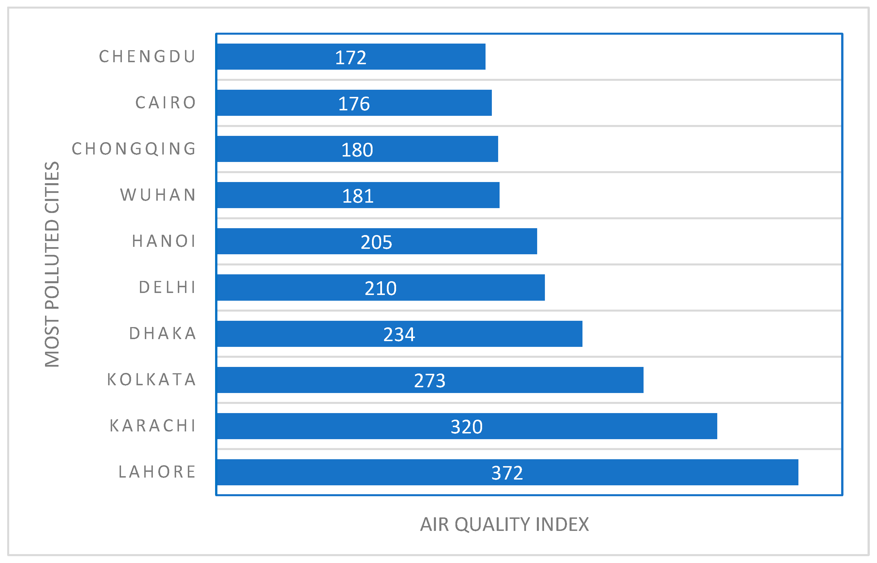
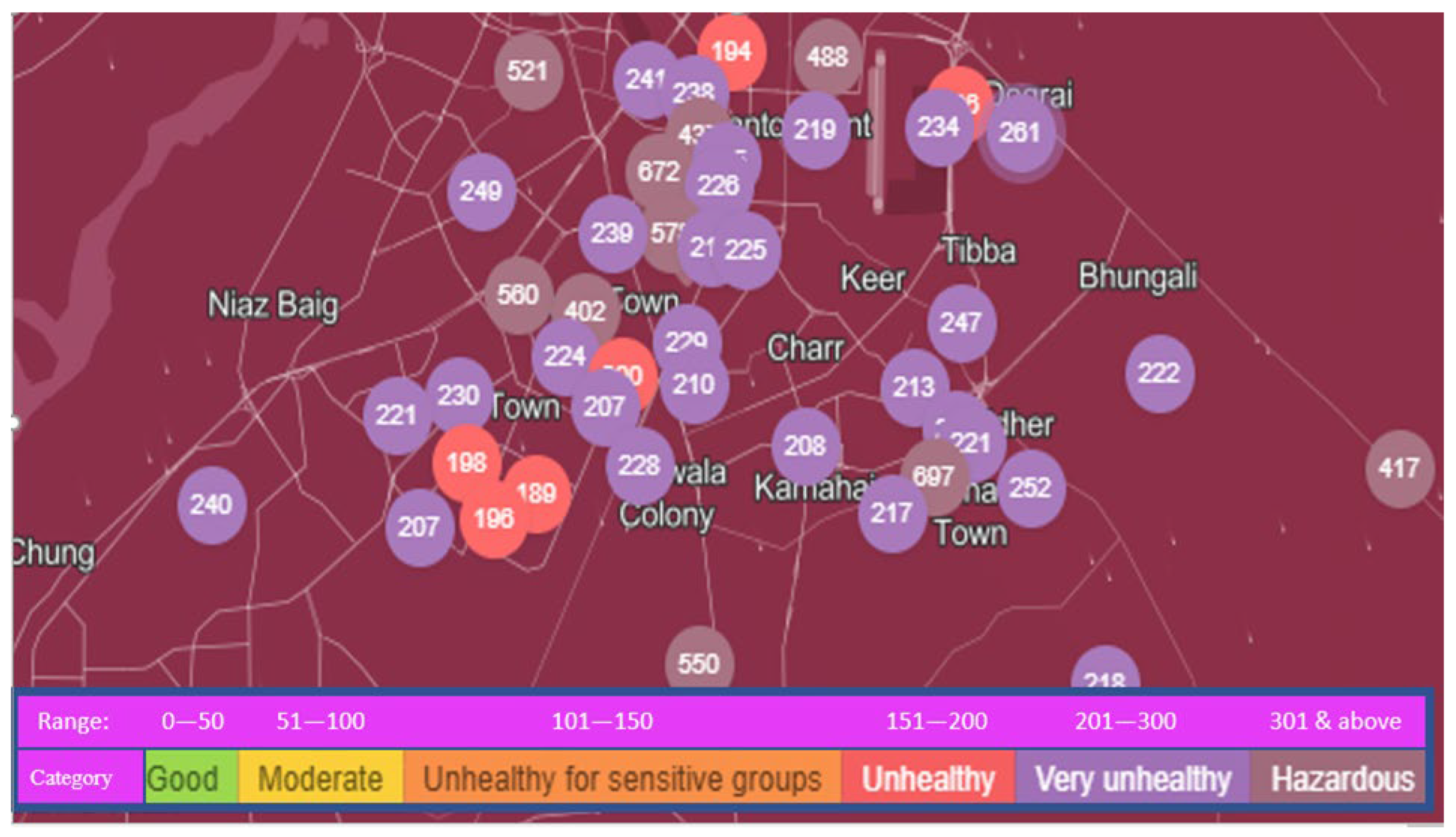
Urban air quality has declined alarmingly in many parts of the world, especially in south Asian cities with high population densities. Lahore, Karachi, Kolkata, Dhaka, Delhi and Hanoi regularly rank at the top of global pollution indices, with particulate matter concentrations frequently exceeding World Health Organization (WHO) guidelines, according to annual assessments from international environmental agencies [1]. Lahore (a city in Pakistan and the capital of the Punjab province) is particularly noteworthy among these as a recurrent hotspot, regularly reporting Air Quality Index (AQI) levels in the dangerous range, especially during winter seasons. These recurrent trends draw attention to both a local environmental catastrophe and the pressing need to comprehend the fundamental reasons that why smog forms in metropolitan areas [2,3]. The world’s highest annual particulate matter concentrations are still found in cities in East Asia, South Asia, and the Middle East; this issue is frequently brought up in international literature. Research from Beijing, Shanghai, and Tehran emphasizes the intricate interaction between anthropogenic emissions and meteorological conditions that propels the development of smog, underscoring the nonlinear character of pollution dynamics [4,5,6]. According to global evaluations, smog is rarely caused by a single source but rather results from a complex interplay between local topography, emission intensities, and climatic conditions. The periodic outbreaks of severe air pollution in south Asia have raised the current study’s scope in the region. During peak pollution months, Lahore has consistently recorded particulate matter (PM_2.5) levels that are 15–20 times higher than the WHO guidelines [7]. Studies from India (Kolkata and Delhi) identify vehicular emissions, industrial activity, biomass burning, and agricultural residue combustion as major contributors [8,9,10]. The air quality findings have been documented for Lahore, where transportation, industrial estates, brick kilns, and crop stubble burning play significant roles in seasonal pollution spikes [11,12]. Furthermore, numerous studies on air transport have shown that the transboundary movement of pollutants across the border between India and Pakistan exacerbates the intensity of smog [13,14]. Figure 1 shows the list of the most polluted cities in the world according to the air quality index [15]. By displaying the AQI measurements recorded in several Lahore locations on 24 November 2025, Figure 2 depicts the regional variations in air quality [16].

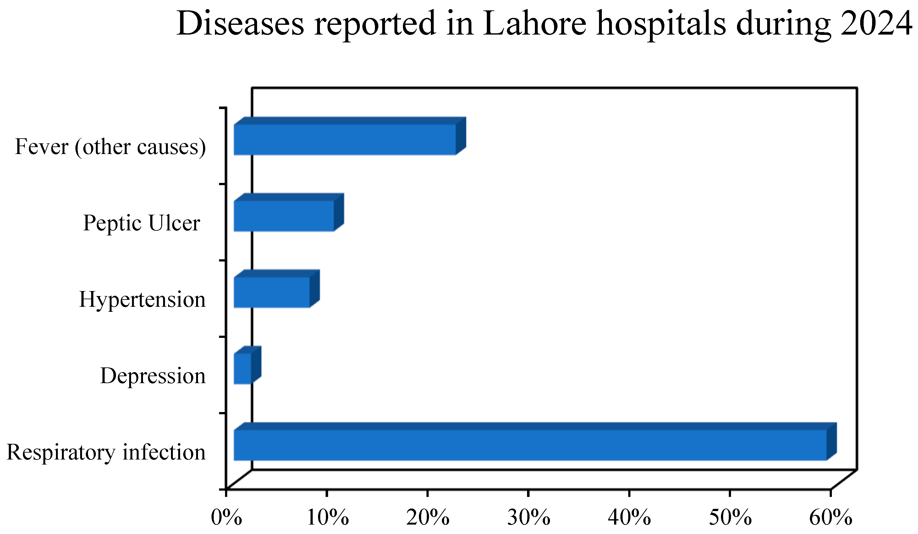
Lahore has been selected as the case study for the current research due to the city’s significant increase in smog severity over the past decade. Extreme pollution episodes now happen every year, posing serious public health concerns. According to recent data, Lahore’s poor air quality causes thousands of premature deaths annually, along with sharp increases in respiratory infections, cardiovascular problems, asthma flare-ups, Chronic obstructive pulmonary disease (COPD) prevalence, and decreased lung function among vulnerable groups like children, the elderly, and outdoor workers [17]. These findings are consistent with epidemiological data from Bangkok, Jakarta, Delhi, and other polluted megacities [18,19]. Smog has detrimental consequences not only on health but also on Lahore’s economy and healthcare system, increasing socioeconomic vulnerability and resulting in lost productivity and long-term medical expenses. Figure 3 shows the illnesses associated with exposure to air pollution in Lahore in 2024. The statistics make it evident that respiratory conditions are the most often reported disease in Lahore [17]. The significant health concerns imposed by deteriorating air quality are highlighted by the fact that chronic illness is either directly linked to or made worse by extended exposure to particulate matter and other airborne contaminants.

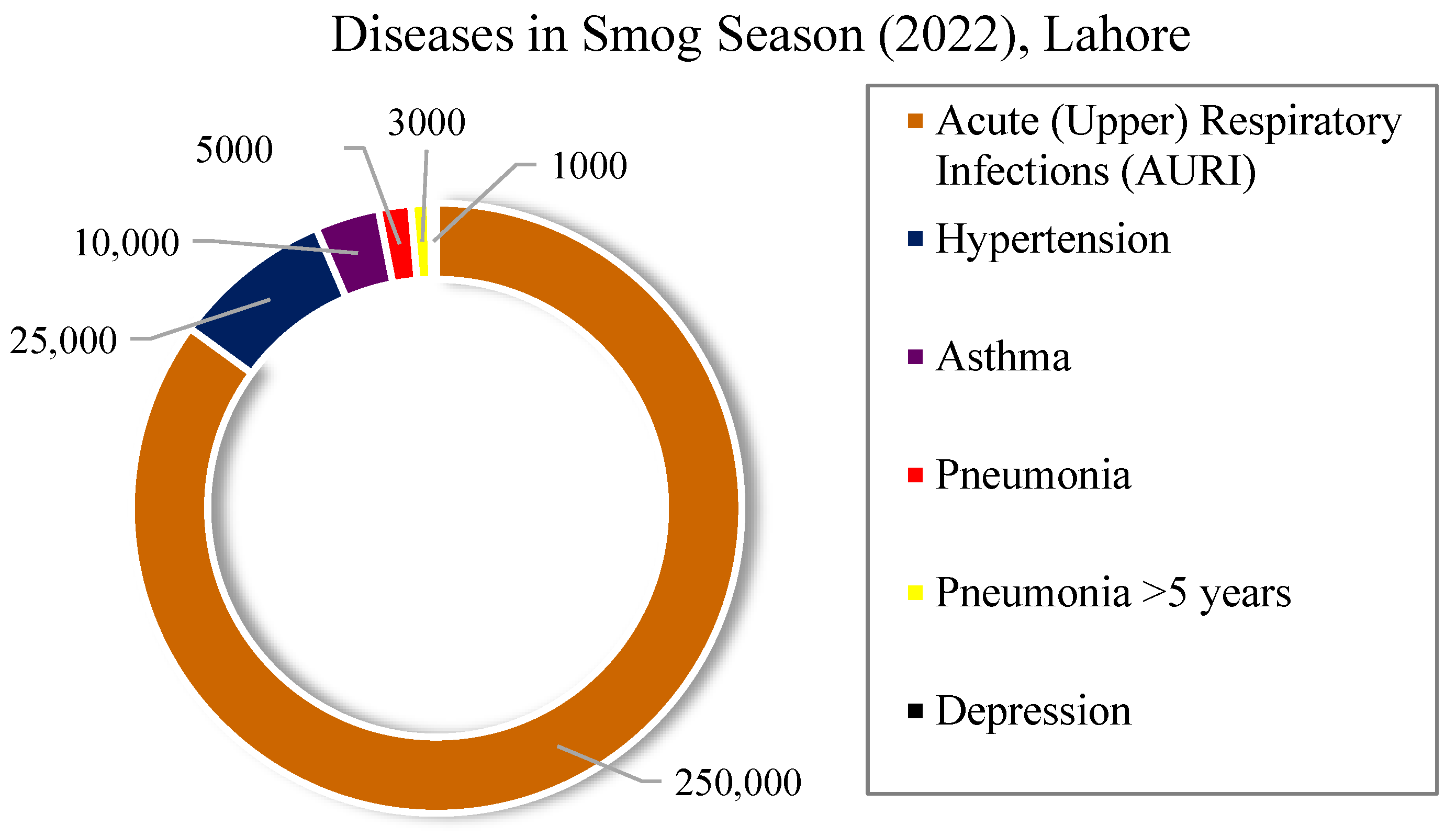
The disease pattern observed in Lahore during the smog season is depicted in Figure 4. According to data from the 2022 smog season, Lahore’s health is significantly impacted by air pollution, with Acute Upper Respiratory Infections (AURI) being the most reported ailment (250,000 cases). Asthma (10,000 instances), pneumonia (5000 cases), and hypertension (25,000 cases) are also prevalent, indicating the close connection between poor air quality and respiratory or cardiovascular stress. Further evidence that smog has an impact on all facets of health comes from additional incidences of depression (1000) and pneumonia in children over five (3000). Overall, the findings verify that respiratory ailments dominate the city’s pollution-related disease patterns [20].

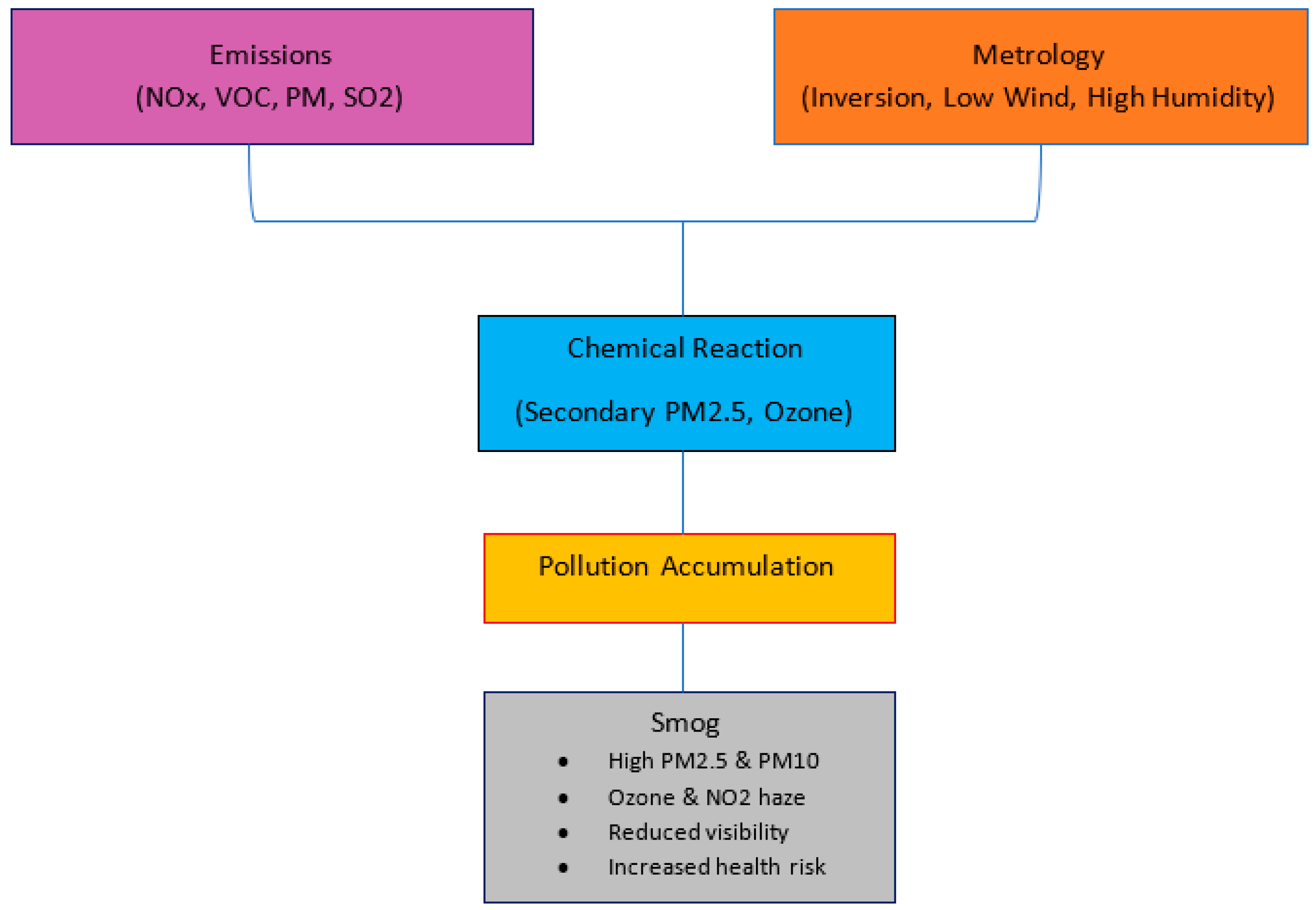
The impact of meteorological conditions on smog entrapment is also extensively studied in the literature. Pollutant dispersion is severely restricted both vertically and horizontally by temperature inversions, low wind speeds, high humidity, and little precipitation. Numerous studies attest to the fact that stable air layers that trap pollutants close to the surface cause particulate matter concentrations to rise sharply during the winter. AQI patterns are shaped by the strong interactions between these climatic phenomena and anthropogenic emissions, including traffic density, industrial fuel combustion, urban congestion, and agricultural burning cycles. The process of smog development caused by emissions and meteorology is depicted in Figure 5. Nevertheless, despite the volume of studies, most studies only look at emission or meteorological aspects separately rather than understanding them as interrelated components of a single atmospheric system.

Table 1. Impact of smog constituents on human health and their control measures.

Smog Constituents	Type	Sources	Impact on Human Health	Mitigation and Control Measures
PM2.5 [21]	Primary	Exhaust emissions, secondary formation from SO2, VOCs, and NOx,	Cardiovascular disease, lung cancer, COPD, and premature death	Stringent emission standards, biofuels, diesel particulate filters, and renewable energy applications
PM10 [22]	Primary	Construction, Agriculture, Mining and Road dust	Bronchitis, respiratory infections, and asthma	Construction regulation, dust suppression, and green buffers
Nitrogen Oxides [23,24]	Primary	High-temperature combustion (Automotives or power plants)	Lung damage, Asthma, and airway inflammation	Selective catalytic reduction and low NOx burners
Carbon Monoxide [25,26]	Primary	Incomplete fuel combustion (Automotives or power plants)	Heart stress, Oxygen deprivation, sudden faint, Headaches, serious poisoning	Effective traffic management and Catalytic converters
Sulphur Dioxide [27,28]	Primary	Smelting, coal combustion, and oil refining	Bronchitis, respiratory infections, and asthma	Low-Sulphur fuels, and Flue-gas desulfurization
Carbon Dioxide [29]	Primary	Fossil fuel combustion, Industrial activities	Cognitive impairment, Cardiovascular Effects, and Mental Health issues	Effective energy management, renewable energy applications, and carbon capture
Ammonia [30,31]	Primary	Livestock, Agriculture, and fertilizers,	Lung and Eye irritation, PM2.5 development	Effective fertilizer management and Stringent emission standards
Volatile Organic Compounds [32,33]	Primary	Automotive exhaust, paints, solvents, and fuel evaporation	Cancer and respiratory irritation	Effective vapor recovery systems and lower concentration VOC products
Ammonium Nitrate/Ammonium Sulphate [34,35]	Secondary	Reaction between ammonia and NOx, SOx	Lung Inflammation and Cardiovascular Effects	Integrated control of NH3, NOx, and SO2
Polycyclic Aromatic Hydrocarbons [36,37]	Primary	Incomplete fuel combustion	Carcinogenic	Cleaner combustion and emission filters
Ground-Level Ozone [38,39]	Secondary	Reaction of VOCs and NOx in sunlight	Asthma and lung damage	NOx and VOC reduction, and emission control
Heavy Metals (Pb, As, Hg, and Cd) [40,41]	Primary	Industrial exhaust and waste incineration	Neurological damage, cancer, and kidney issues	Effective industrial emission control and waste management

reports the constituents of smog affecting human health and their control measures. PM_2.5 [21] is a primary constituent of smog originating from exhaust emissions, secondary formation from SO₂, VOCs, and NO_x. It results in cardiovascular disease, lung cancer, COPD, and premature death. The stringent emission standards, biofuels, diesel particulate filters, and renewable energy applications can play their role in the reduction of PM_2.5 from the atmosphere. The primary constituents of smog, like NO_x, SO_x, CO_x, and ammonia, are directly emitted into the environment mainly due to automotive and industrial effluents. They are responsible for asthma, neurological disorders, cancer, lung diseases, cognitive impairment, cardiovascular diseases, and premature mortality. However, the secondary smog constituents like ozone and ammonium sulphate/nitrate are produced from the chemical reaction between primary pollutants in the presence of sunlight. They are mainly responsible for cardiac and lung diseases. The integrated emission control techniques and improved agriculture management can improve air quality.

Machine learning (ML)-based methods for modeling air quality have been increasingly popular in recent years. Because they can capture nonlinear relationships and high-dimensional interactions, techniques like Random Forest and Gradient Boosting have shown greater prediction performance over conventional statistical methods. While some research concentrates on pollutant-specific prediction frameworks, others show the potential of ML for forecasting AQI using meteorological variables. However, a significant drawback is that many of these models are difficult to understand or do not incorporate meteorological and emission parameters collectively. These study gaps are particularly noticeable for Lahore, where there are still few thorough, data-driven pollution evaluations. Studies that combine meteorological and emission parameters, use high-accuracy machine learning models, and incorporate interpretability are desperately needed to identify the main sources of pollution. Closing these gaps is essential for establishing focused and successful mitigation plans. Driven by these limitations as well as increasing health and environmental problems in Lahore, the current work intends to develop prediction tools to assist evidence-based policymaking while analyzing, modeling, and comprehending the fundamental causes of smog generation. Smog, PM_2.5, PM₁₀, NO_x, oxides of sulphur (SO₂), ozone, carbon monoxide (CO), and volatile organic compounds (VOCs) are caused by a variety of emission sources, including burning of agricultural residue, industrial activities, domestic fuel usage, and vehicle activity. Temperature, humidity, wind speed, pressure, and precipitation all influence the atmospheric behavior. Therefore, the combination of climatic conditions and emission inventories is necessary for a thorough assessment. Additionally, this research contributes to Sustainable Development Goals (SDGs 3), named as Good Health and Well-Being and SDG 11, named as Sustainable Cities and Communities, which are worldwide priorities for environmental sustainability and public well-being. It aims to assist resilient urban planning and enhance data-driven decision-making by providing analytical tools and prediction models.

Table 2. Recent analysis on air pollutants and smog through machine learning models.

Reference	Location	Scope	ML Model Used	Findings
[42]	Delhi, India	Air quality monitoring using temp, humidity, wind for PM only	Random forest (RF) and Adaboost Models	Accuracy for Adaboost reaches 98.24% which is highest among all the models
[43]	Lahore, Pakistan	Analyze pollutants to determine main cause for respiratory diseases	RF, XGBoost, Logistic Regression Models	The models had been identified to be very accurate, F1-score, and area under the receiver operating characteristic curve (ROC-AUC) measures. PM2.5 and PM10 are found to be the main cause of respiratory and other health problems
[44]	Lahore, Pakistan	Predictive model to forecast PM2.5 and PM10	Artificial Neural Network (ANN) Model	Model’s high accuracy (>90%) in predicting air quality indices and identifying critical thresholds for smog
[45]	Delhi, India	Predictive model for PM2.5 forecast	RF, ANN, Supervised machine learning (SVM) Models	RF gave the best results for both training and testing. Testing accuracy (coefficient of determination (R2) = 0.842, root mean square error (RMSE) = 0.06, and mean absolute error (MAE) = 0.045)
[46]	Delhi, India	Predictive method to examine and measure how stubble burning affects air pollution	Gradient Boosting Regression Model	AQI change per 1% fire count increase varies between 0.08% and 0.38%, showing a consistent but varying impact.
[47]	Hong Kong	Develop machine learning-based models for predicting hourly street-level PM2.5 and NOx concentrations	RF, boosted regression tree (BRT), SVM, XGBoost, Generalized additive model (GAM), and Cubist Models	RF outperformed other machine learning algorithms (MLAs) with ten-fold cross-validation (CV) R2 values higher than 0.81 and 0.62 for PM2.5 and NOx predictions, respectively.
[48]	Macau	Develop a dependable air pollution prediction model for Macau	RF, support vector regression (SVR), ANN, Recurrent Neural Networks (RNN), Long Short-Term Memory (LSTM), Gated recurrent units (GRU) Models	The RF model best predicted PM10, PM2.5, NO2, and CO concentrations with the highest Pearson Correlation Coefficient (PCC) and Kendall’s Tau Coefficient (KTC) in a daily air pollution prediction
[49]	Eastern China	Predictive model for daily NO2 concentrations	XGBoost Model	R2 of 0.75 and root-mean-square error (RMSE) of 9.11 μg/m3
[50]	Lahore, Pakistan	Predictive model for Aerosol optical depth (AOD) used to estimate the extent of air pollution	SVR and SVR-Grey Wolf Optimisation (GWO) Models	SVR-GWO model (RMSE = 0.07, MAE = 0.06, R2 = 0.6) performed better than others
[51]	Dhaka, Bangladesh	Prediction model for the ground-level PM2.5 concentrations	Regression Tree (RT), Additive Regression (AR), Reduced Error Pruning Tree (REPT), Random Subspace (RSS) Models	The RSS model is the most suitable model for PM2.5 prediction, as shown by the lower MAE and RMSE values and a higher R2 value
[52]	Almaty, Kazakhstan	Prediction model for the ground-level PM2.5 concentrations	RNN, LSTM Models	LSTM is better at forecasting for 90 days (MAE = 2.0, mean absolute percentage error (MAPE) = 11.57, RMSE = 2.18)
[53]	Visakhapatnam, India,	Prediction model for AQI	RF, Catboost, Adaboost, and XGBoost Models	Catboost and RF models performed best, showing maximum correlations of 0.9998 and 0.9936

compares the analysis conducted in previous studies on air pollutants and smog.

Recent research that has thoroughly examined the application of machine learning (ML) models for forecasting air quality and determining the main causes of pollution is compiled in Table 2. Models like Random Forest (RF), AdaBoost, Gradient Boosting Regression (GBR), and Artificial Neural Networks (ANN) have been used in India to predict particulate matter (PM_2.5 and PM₁₀) and evaluate the effects of stubble burning. AdaBoost achieved the highest accuracy of 98.24%, while RF performed better in PM_2.5 prediction [42,45,46,53]. Studies conducted in Pakistan using RF, XGBoost, Logistic Regression, and ANN models to assess pollutants and forecast air quality indices have found that PM_2.5 and PM₁₀ are major causes of respiratory diseases, with prediction accuracy surpassing 90% [43,44,50]. Like this, ensembles of machine learning models, such as RF, Boosted Regression Trees (BRT), SVM, XGBoost, GAM, Cubist, and recurrent neural networks like RNN, LSTM, and GRU, have been used for daily and street-level air pollutant forecasting in Hong Kong, Kazakhstan, and Macau. Based on cross-validation metrics and correlation coefficients, RF consistently outperforms other models [47,48,52]. Furthermore, the research in Dhaka showed that Random Subspace (RSS) models are very successful for PM_2.5 forecasting, while XGBoost and SVR variations have been successfully employed in Eastern China and Lahore for NO₂ and Aerosol Optical Depth (AOD) prediction [49,50,51]. Overall, these investigations demonstrate the adaptability and strong predictive power of both conventional and deep machine learning models in identifying non-linear connections, temporal patterns, and pollutant-specific impacts in air quality datasets from various geographical locations. All things considered, ensemble models like RF and XGBoost frequently outperformed other machine learning and deep learning techniques in predicting air quality indices and pollutant concentrations, consistently demonstrating higher predictive accuracy across numerous experiments. These models were chosen for the current investigation primarily for this reason.

Despite substantial research on air quality, a critical gap remains in integrating emissions and meteorological factors as interdependent components of the atmospheric system. As summarized in Table 2, most previous studies focus on either pollutants or meteorological parameters in isolation. For instance, Pervaiz et al. [43] analyzed multiple pollutants in Lahore to identify PM_2.5 and PM₁₀ as the main contributors to respiratory diseases, but the interactions with meteorological conditions were not fully considered. Similarly, Komal et al. [50] predicted Aerosol Optical Depth using SVR and SVR-GWO, incorporating some atmospheric parameters but without jointly modeling pollutant dynamics. Similar trends can be observed in the studies reported in India [42,45,46,53], Hong Kong [47], and Punjab [44], using machine learning approaches to predict meteorological factors or individual pollutants, with very few studies portraying their integrated impacts. Although these studies offer insightful information, there is still a dearth of Lahore-specific research. This emphasizes the need for further targeted research to fully explain the production of smog, pinpoint important causes, and guide practical mitigation techniques. By integrating emissions and meteorological variables into a single machine learning framework for Lahore, our study closes this gap and offers more precise, useful insights into the dynamics of urban haze.

Smog is a complicated atmospheric phenomenon that results from the interaction of many emission sources and the current weather. Particulate matter (PM), which includes fine solid or liquid particles like PM_2.5 (≤2.5 µm) and PM₁₀ (≤10 µm), is one of its main components. These particles cause smog, respiratory issues, and reduced visibility. Nitrogen oxides (NO_x) are mostly released by industrial processes, power plants, and automobile traffic. Equation (1) shows the formation of NO because of the reaction between nitrogen and oxygen. The resulting NO on further reaction with oxygen forms NO₂ (see Equation (2)).

$$N_2+O_2\to 2NO$$

(1)

$$2NO+O_2\to 2N{O}_2$$

(2)

When exposed to sunlight, NO_x combines with volatile organic compounds (VOCs) to produce secondary particulate matter (see Equation (3)) and ozone (see Equation (4)).

$${NO}_2+h\upsilon \left(light\right)\to NO+O$$

(3)

$$O+O_2\to O_3$$

(4)

VOCs, which originate from biogenic sources, industrial solvents, and fuel burning, are essential to the development of photochemical smog. While ozone (O₃) develops as a secondary pollutant from the photochemical interaction of NO_x and VOCs and frequently dominates the composition of photochemical smog, sulphur dioxide (SO₂), which is mostly generated from the combustion of coal and oil, creates secondary sulphates that contribute to acid smog. The bloodstream’s ability to carry oxygen is hampered by carbon monoxide (CO), a byproduct of incomplete combustion. Other trace gases, including CO₂, methane, and ammonia, also influence atmospheric chemistry (see Equation (5)).

$$2C+O_2\to 2CO$$

(5)

Smog is traditionally divided into two categories: photochemical (Los Angeles-type) smog, which is dominated by NO_x, VOCs, and ozone in warm, sunny areas with heavy traffic, and classical (London-type) smog, which is defined by elevated sulphur compounds and PM under cold, humid conditions with coal or industrial emissions. Smog episodes in Lahore are usually a hybrid situation where the main contributors to winter pollution occurrences are PM, NO_x, and ozone. A meteorological phenomenon known as temperature inversion occurs when a layer of warm air covers cooler air close to the surface, preventing the typical vertical drop in temperature with altitude that promotes the dispersal of pollutants. Cooler air is trapped beneath the warmer layer during an inversion, which prevents vertical mixing and causes pollutants from burning biomass, industrial activities, and vehicle traffic to build up close to the ground. Due to increased levels of particulate matter (PM), nitrogen oxides (NO_x), carbon monoxide (CO), and other smog constituents, the Air Quality Index (AQI) rises noticeably. Long-lasting inversions, which often occur during winter mornings and nights, intensify smog sections, resulting in notable reductions in visibility and heightened risks to public health. Between October and November, when calm breezes, high emissions, and low nighttime temperatures all combine to produce persistent, dense smog, these inversions are particularly evident in Lahore. These dynamics demonstrate the critical role that meteorological factors, such as wind speed, temperature, and humidity, play as significant predictors in machine learning models for AQI, as confirmed by the current study’s findings. To accurately predict AQI and quantify the relative contribution of each factor to smog formation, this study aims to develop a dual analytical framework that: (i) integrates meteorological and emission factors using machine learning models (Random Forest and XGBoost); and (ii) identifies the key sectors responsible for major pollutant emissions, providing interpretable insights to support evidence-based policymaking and targeted smog mitigation strategies in Lahore.

The current study introduces methodological novelty through the development of a unified and interpretable machine-learning framework that jointly addresses AQI prediction, systematic model-based attribution, and sector-level impact analysis for Lahore, which is one of the most severely smog-affected megacities globally. Most of the existing studies primarily focus on optimizing predictive accuracy in isolation. The current study suggests a methodology that explicitly combines forecasting performance with an organized assessment of the relative contributions of meteorological conditions and emission-related variables within a single, transparent, location-specific analytical pipeline. The framework provides strong, city-specific insights into key AQI-associated factors for Lahore, a context that is still relatively understudied in the existing literature, by fusing prediction with interpretable attribution and sector-oriented analysis. As a result, the current work moves beyond standalone prediction into a coherent, interpretable, and policy-relevant analytical framework, advancing the use of machine-learning techniques in air-quality research.

2. Materials and Methods

The current study is conducted in two stages to ascertain the causes of smog development in Lahore, Pakistan, during the winter months of October and November, which have traditionally been linked to significant declines in the region’s air quality. The impact of aggregated emission sources and meteorological factors on AQI variation is investigated in the first phase. To identify the sector-wise pollutants that most significantly contribute to the creation of smog, the second phase concentrated on the chemical makeup of emissions, specifically CO₂, NO_x, VOC, and particle matter. Machine learning methods are used for all studies to guarantee interpretability and forecast accuracy. Daily readings of AQI, temperature, wind speed, and total emissions mostly attributable to automobiles and industrial activity were included in the dataset. These observations are gathered from a variety of official repositories and reliable internet sources [16,20,54]. Incomplete entries are eliminated, units are confirmed, and variables are aligned to a consistent daily period to clean up the dataset. Correlation matrices and scatter plots are used in feature exploration to find initial connections between AQI and explanatory variables. The nonlinear and multidimensional association between the environmental parameters and AQI is modeled using two machine learning models: Random Forest Regressor and XGBoost Regressor. RMSE and R² are used to assess the model’s performance after the dataset was divided into training (80%) and testing (20%) subsets. The relative contributions of climatic variables and emission sources on smog intensity are ranked using feature relevance ratings and regression coefficients. The model’s generalization and reliability are assessed using residual diagnostics and actual-versus-predicted graphs. Data is examined for smog elements at the next stage. Vehicle emissions, industry emissions, and agriculture emissions are the top three sources of emissions that were examined. For every source, calculations are made for particulate matter (PM), nitrogen oxides (NO_x), carbon dioxide (CO₂), and volatile organic compounds (VOCs).

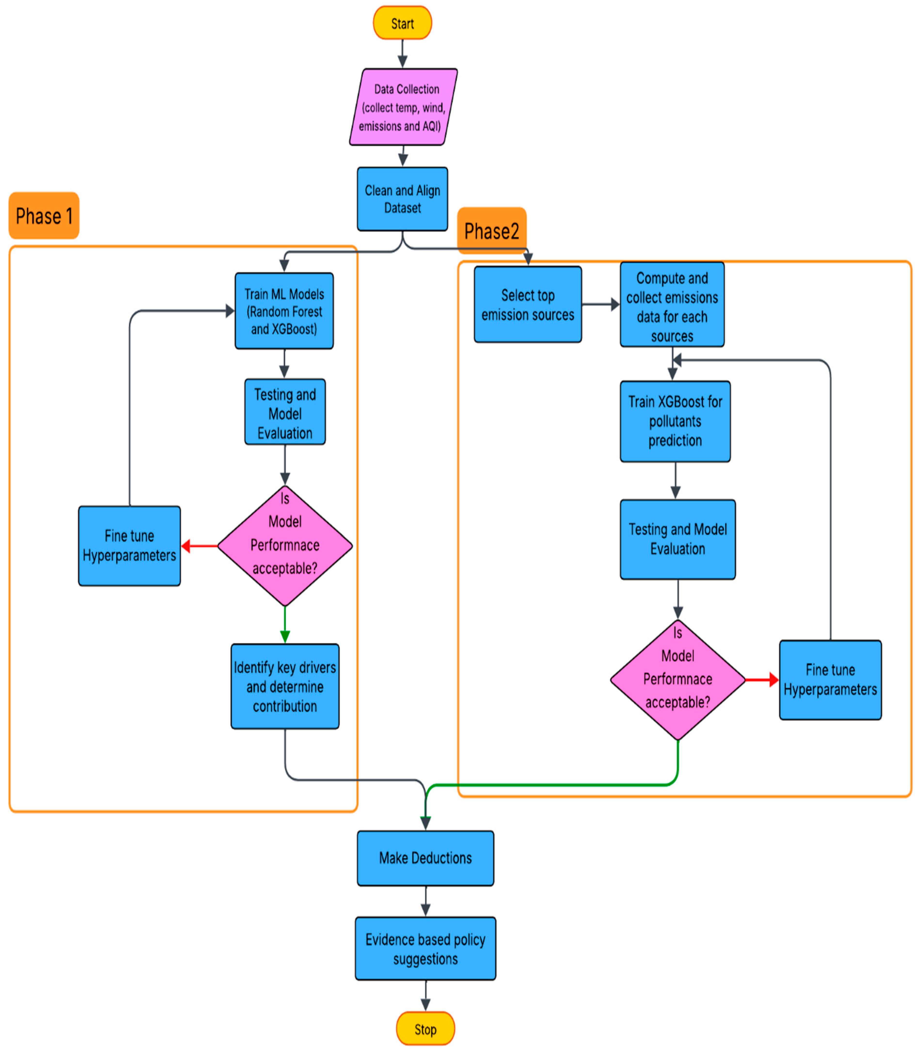
Non-linear correlations in the data are precisely predicted and captured by the XGBoost model. Model performance is further evaluated using a 3-fold cross-validation for a more realistic assessment, making sure that each fold maintains the temporal order of the data to avoid leaking. The model’s performance is evaluated and compared using RMSE and R² metrics. Google Colab is used to do all analyses in Python 3.10. Scikit-learn (v1.3.2), XGBoost (v2.0), Pandas (v2.1), NumPy (v1.26), Seaborn (v0.13), and Matplotlib (v3.8) were among the libraries. This two-tiered analytical technique not only predicts AQI with high accuracy but also sheds light on the relative contributions of chemical contaminants, emission sources, and meteorological factors to AQI fluctuation in Lahore. The current study provides an organized framework for examining patterns of smog generation and guiding evidence-based conversations about possible mitigating measures. Figure 6 illustrates the flowchart of the methodology adopted in this study.

2.1. Experimental Set-Up

Two different datasets representing smog drivers in Lahore in October and November are used in the study: (i) meteorological parameters combined with total emissions from vehicles and industry, and (ii) chemical composition of vehicular, industrial, and agricultural emissions, including CO₂, NO_x, VOC, and particulate matter (PM). Weather information, emission inventories, and official air quality monitoring stations are the data sources. When necessary, features are standardized, especially for the machine learning models, and all datasets are pre-processed to eliminate missing or unusual values. Correlation matrices, scatter plots, and pairwise distributions are used in exploratory data analysis to find early correlations and possible multicollinearity among variables.

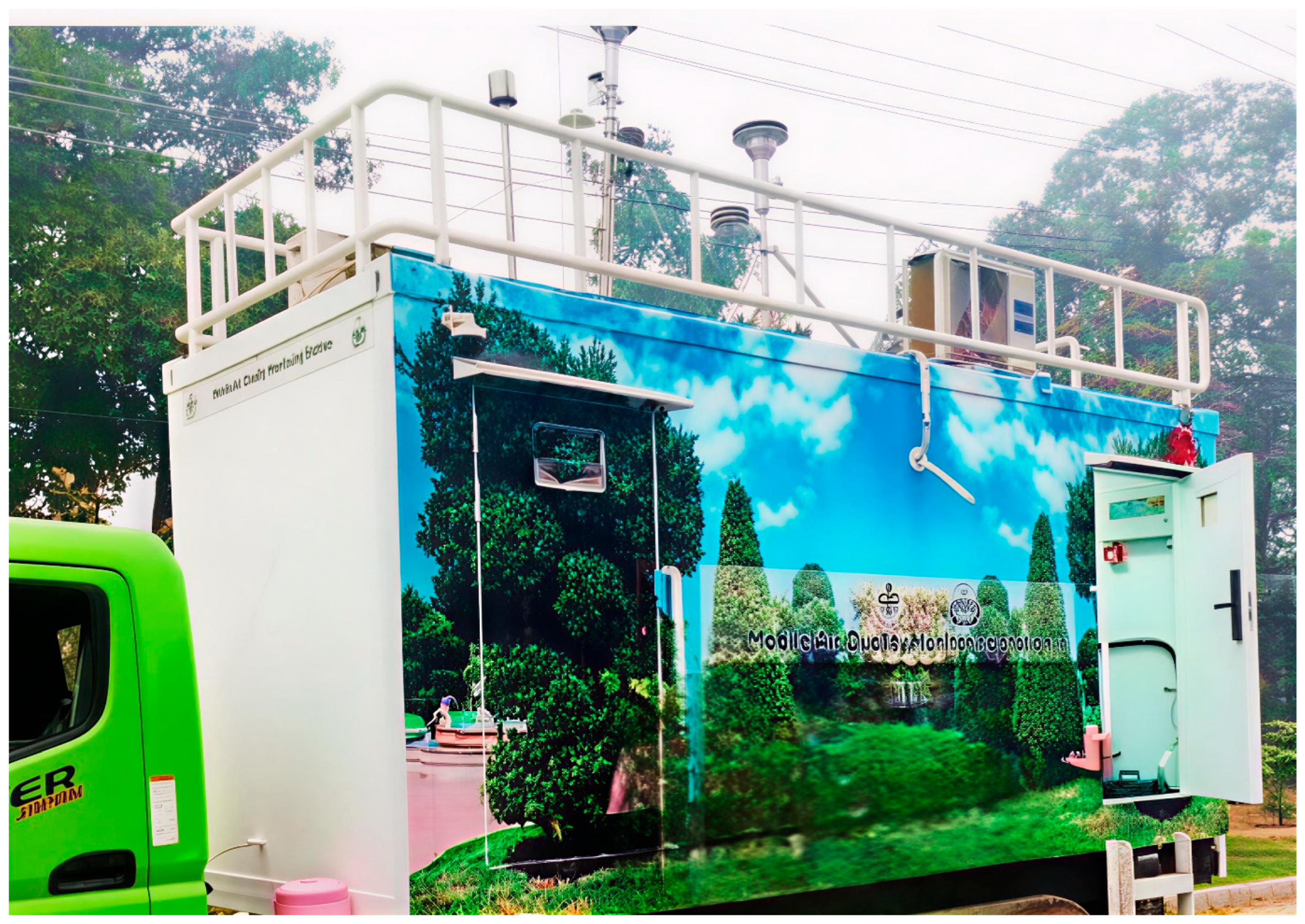
Air quality data for Lahore are obtained from The Urban Unit, Government of Punjab, using 10 monitoring stations, comprising 8 fixed stations and 2 mobile stations, strategically distributed across major urban areas to provide point-based measurements with adequate spatial coverage. The stations recorded hourly concentrations of multiple pollutants, including PM_2.5, PM₁₀, NO_x, CO, and VOCs, along with the Air Quality Index (AQI). To ensure a consistent depiction of overall air quality, hourly data is combined into daily averages at each site and then averaged across all stations to get daily AQI values for the entire city. At least 184 citywide observations were made during the study period, which ran from October to December in 2024 and 2025. The daily AQI for the entire city is calculated by averaging the data from all ten stations. Linear interpolation was used to impute missing data (less than 5% of observations). This dataset offers enough temporal and spatial coverage to assess model performance and analyze citywide AQI changes. A mobile air quality station in Lahore is depicted in Figure 7.

Before being deployed, every sensor is factory-calibrated by the manufacturer to guarantee baseline accuracy. The Urban Unit’s regular quality assurance (QA) and quality control (QC) procedures, which include routine inspections, drift monitoring, and baseline adjustments, were followed while the sensors were in use. The monitoring stations are housed in ventilated enclosures to minimize environmental influences such as direct sunlight and precipitation. Pollutant concentrations are sampled at an hourly frequency throughout the study period. Hourly measurements are first aggregated into daily averages at each station, and the city-wide daily AQI is subsequently computed by averaging across all 10 stations. Daily data are publicly available on the official Urban Unit webpage. The monitoring network employs continuous instruments typical of regulatory AQI systems, including Beta-Attenuation Monitors (BAM) for particulate matter and regulatory-grade gas analyzers for NO_x and CO. A station in Lahore also operates a United States (US)-Environmental Protection Agency (EPA)-certified BAM-1020 for PM_2.5 measurements. Meteorological sensors for temperature and humidity are also included to support AQI computation.

The dataset is divided into training (80%) and testing (20%) subsets for predictive modeling using random sampling and a fixed seed to guarantee reproducibility. Two tree-based modeling techniques are used: XGBoost and Random Forest Regressor. The Random Forest models are set up with 100 decision trees, a random seed of 42, and the default mean squared error threshold for node splitting. To reduce overfitting, XGBoost models are trained with 100 estimators, a learning rate of 0.1, a maximum tree depth of 3, and a subsample fraction of 1. To increase prediction performance while maintaining generalization capabilities, preliminary grid searches are used to adjust the hyperparameters for both models. Furthermore, a 3-fold cross-validation split is used for cross validation, guaranteeing that each fold maintained the chronological order of the data to avoid leakage. Several measures, such as Root Mean Squared Error (RMSE), Mean Absolute Error (MAE), and coefficient of determination (R²), are used to evaluate the model. The proportionate contribution of each parameter to AQI variability for tree-based models is determined by extracting feature importance scores. To evaluate model fit and identify potential biases, residual analysis and actual versus projected plots were created. To provide insights for focused smog mitigation methods, scenario studies are also conducted in which specific pollutants (such as NO_x, CO, VOC, and PM) affected emission type and AQI.

Table 3. Model Configurations and Hyperparameters.

Model	Key Hyperparameters/Architecture	Values/Settings
Random Forest Regressor	Number of Trees (n_estimators)	100
	Minimum Samples per Leaf (min_samples_leaf)	1
	Splitting Criterion	Mean Squared Error
	Random Seed	42
XGBoost Regressor	Number of Trees (n_estimators)	100
	Learning Rate (eta)	0.1
	Maximum Depth (max_depth)	3
	Subsample Fraction (subsample)	1
	Random Seed	42

shows the model configuration and hyperparameters.

2.2. Uncertainty

Model uncertainty is quantified using variability in k-fold cross-validation results. Given the use of 3-fold cross-validation, fold-wise R² and RMSE values were first obtained for each validation fold. The mean (μ) and standard deviation (σ) of these metrics are then computed across folds, where σ captures the dispersion in model performance due to data partitioning. Uncertainty is reported as mean ± standard deviation. Uncertainty is computed using the following formula of mean μ (Equation (6)) and standard deviation σ (Equation (7)).

$$\mu ={\displaystyle \frac{1}{K}}{\sum }_{i=1}^K{M}_i$$

(6)

$$\sigma =\sqrt{{\displaystyle \frac{1}{K-1}}{\sum }_{i=1}^K{(M_i-\mu )}^2}$$

(7)

Additionally, 95% confidence intervals were estimated to assess the robustness of predictive performance (see Equation (8)).

$$CI=\mu \pm t_{\alpha /2,K}\sigma /\surd K$$

(8)

3. Results and Discussion

3.1. Influence of Weather and Emissions on AQI

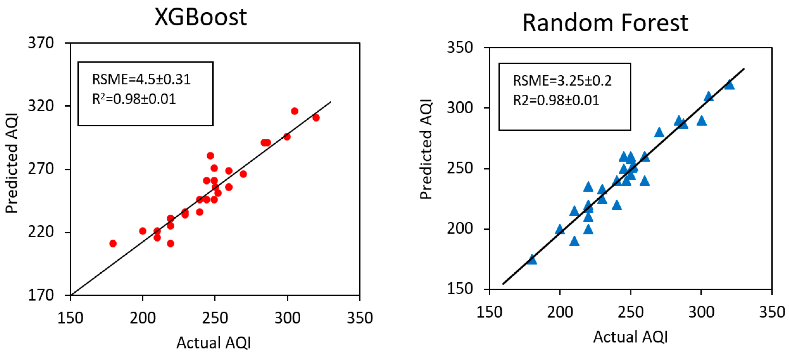
The link between AQI and environmental factors, such as temperature, wind speed, and total emissions from vehicles and industries, is examined in the first phase. The AQI varied significantly between October and November, with daily averages ranging from moderate to extremely hazardous levels, according to descriptive statistics. A comparison of machine learning models for AQI prediction based on emissions and meteorological data is presented in Figure 8. The XGBoost model’s predictive ability for calculating the Air Quality Index (AQI) demonstrates a significant agreement between expected and observed values, as evidenced by the near alignment of data points along the 1:1 line in the scatter plot. The model’s low Root Mean Square Error (RMSE = 4.5) and high coefficient of determination (R² = 0.987) suggest that the model explains roughly 98.7% of the variance in AQI and that projected AQI values deviate very little from actual measurements. The ability of XGBoost to catch intricate nonlinear connections between anthropogenic emissions, including those from industry and automobiles, and meteorological data, like temperature and wind speed, accounts for this high level of precision. While minor deviations from the ideal line indicate localized prediction errors that may arise from temporal fluctuations in emissions or unmodeled environmental conditions, overall, the model provides reliable and robust AQI estimation for the dataset. The Random Forest (RF) model performs similarly to XGBoost with a lower RMSE of 3.3 and a R² of 0.988, indicating a little better fit in terms of variance explanation and smaller total prediction errors. The RF model effectively captures the general patterns in AQI based on meteorological and emission data, demonstrating its suitability for prediction tasks requiring nonlinear and multivariate inputs. However, modest changes in scatter patterns and sensitivity to extreme AQI values may favor XGBoost in situations where accurate capture of variability and rare occurrences is critical. When coupled, both models exhibit high predictive ability, with XGBoost permitting robust modeling of complicated relationships and Random Forest providing a somewhat lower RMSE. This demonstrates the importance of choosing a model based on data attributes and AQI prediction targets.

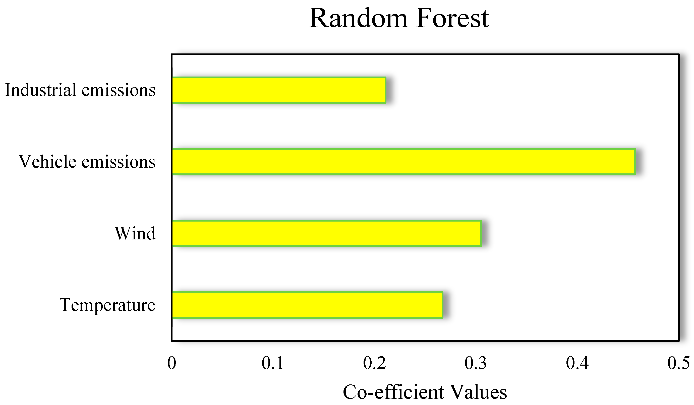
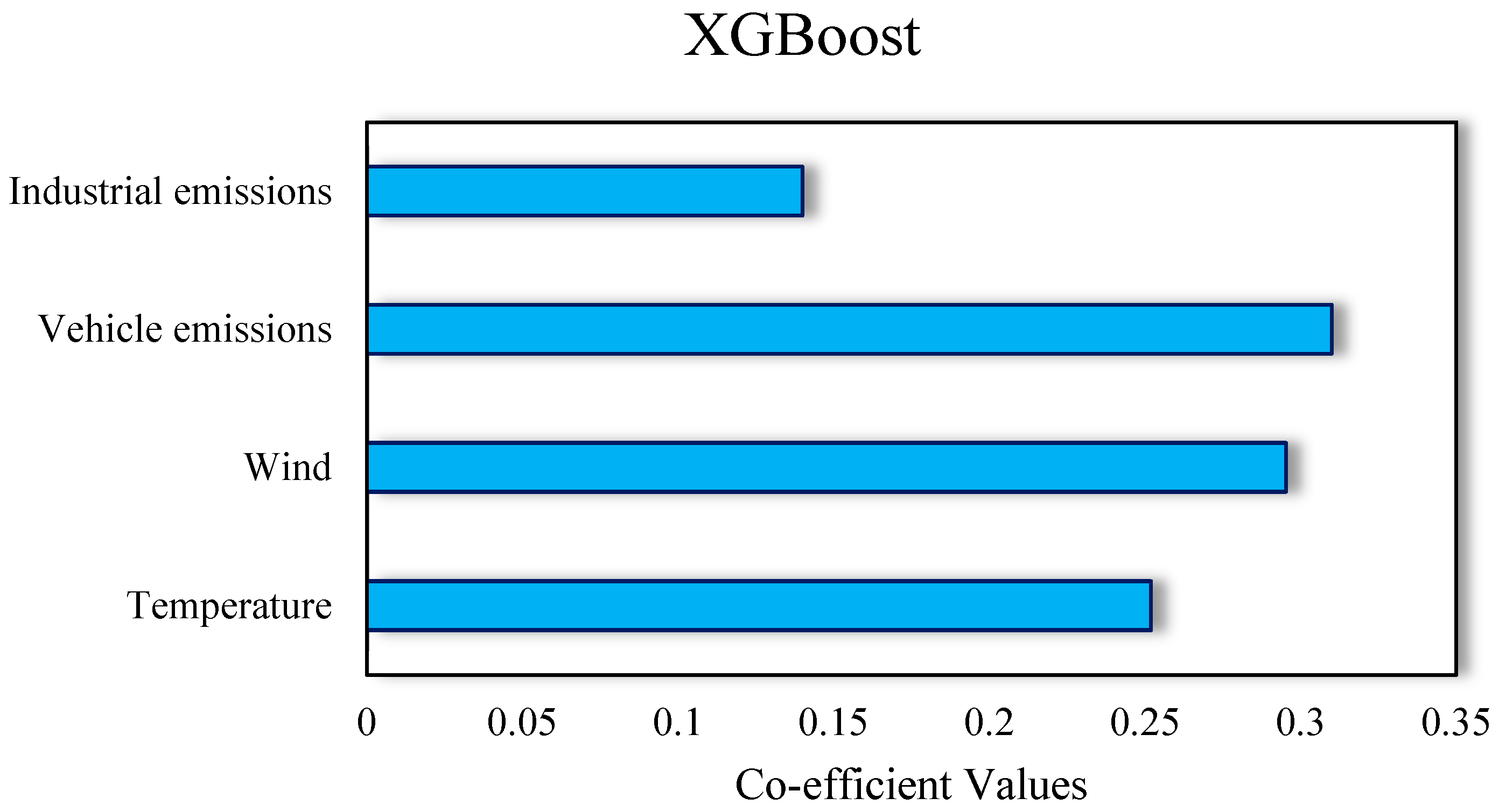
The variations in the relative contributions of meteorological and emission parameters to AQI prediction are revealed by the variable importance analysis of the Random Forest (RF) and XGBoost models. As shown in Figure 9, vehicle emissions had the highest coefficient value (0.46) in the RF model, indicating a significant impact on AQI volatility. Industrial emissions make up the least amount (0.22), followed by wind (0.31) and temperature (0.27). This suggests that the RF model gives direct anthropogenic causes, particularly automobile activity, priority over climatic elements, which have a moderate effect on air quality. In contrast, Figure 10 shows that the XGBoost model has a somewhat different distribution of coefficients. Vehicle emissions continue to be the most important predictor (0.32), but industrial pollutants (0.15) have a considerably smaller impact than in RF, while temperature (0.25) and wind (0.31) contribute more equally. This implies that more intricate interactions between meteorological variables and emissions are captured by XGBoost’s gradient boosting technique, which can represent nonlinear dependencies and inter-variable effects. On the other hand, RF lends more weight to the primary source of pollution (vehicle emissions), while XGBoost distributes impact more evenly among contributing characteristics, demonstrating increased sensitivity to environmental modulators like temperature and wind. Overall, these results demonstrate that while both models recognize vehicle emissions as the main contributor to AQI, XGBoost offers a more comprehensive representation of the combined effects of anthropogenic activities and meteorology, potentially improving prediction accuracy for complex or variable air quality scenarios.

3.2. Effect of Emission Composition

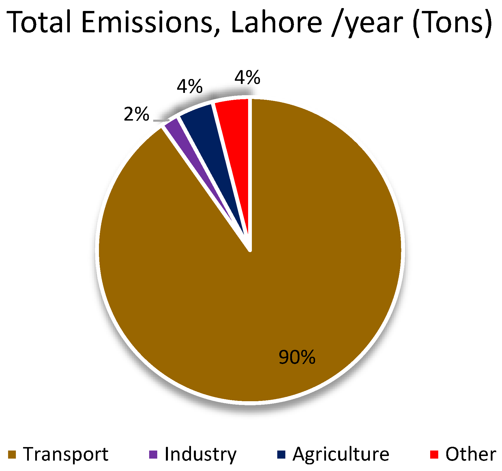
Phase 2 used the XGBoost regression model to examine the impact of individual emission elements on the production of smog. The four main pollutants that contribute to emissions, NO_x, CO, VOC, and PM, are the focus of the analysis. The XG Boost regression model is selected due to the superior predictive ability in structured datasets, and the gradient-boosting mechanism that gradually improves model accuracy, along with the capacity to capture subtle nonlinear pollutant interactions, and improved performance in handling imbalanced or noisy data through built-in regularization, as confirmed by prior research [55,56,57]. The government organization’s disclosed data on real pollutant concentrations made up the dataset [20]. A sector-by-sector breakdown of Lahore’s total annual emissions is shown in Figure 11, which also shows the relative contributions of industry, transportation, agriculture, and other smaller sources. According to the pie chart, transportation emissions account for around 90% of the city’s annual emissions, with the industrial, agricultural, and miscellaneous sectors contributing only 4%, 4%, and 2%, respectively. This unequal distribution highlights the significant role vehicle activity plays in shaping Lahore’s air pollution environment.

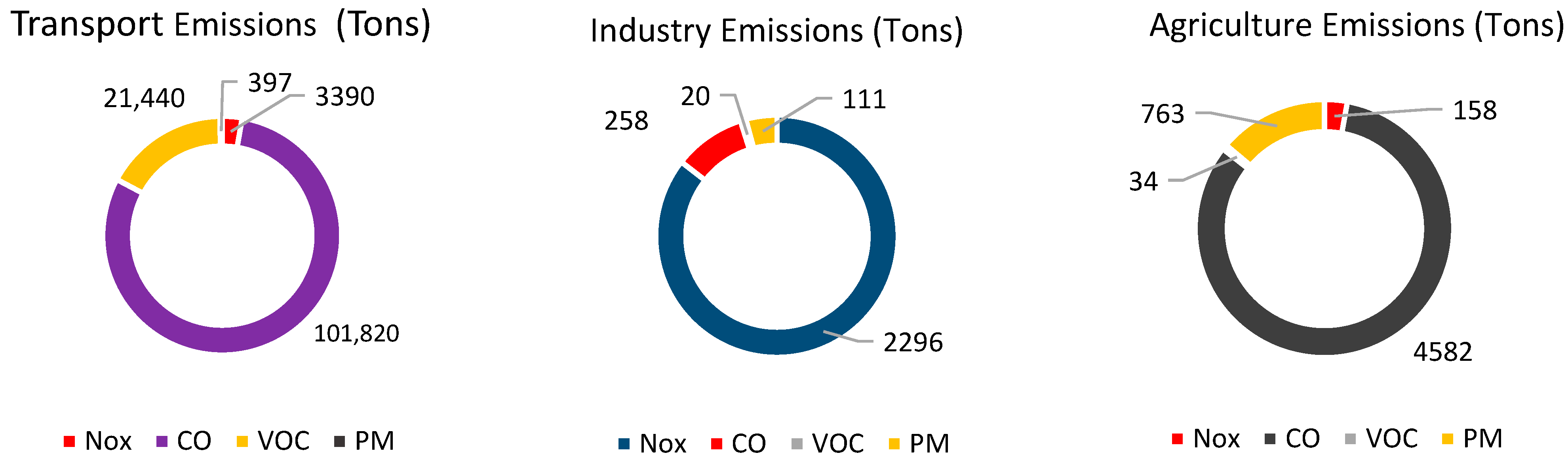
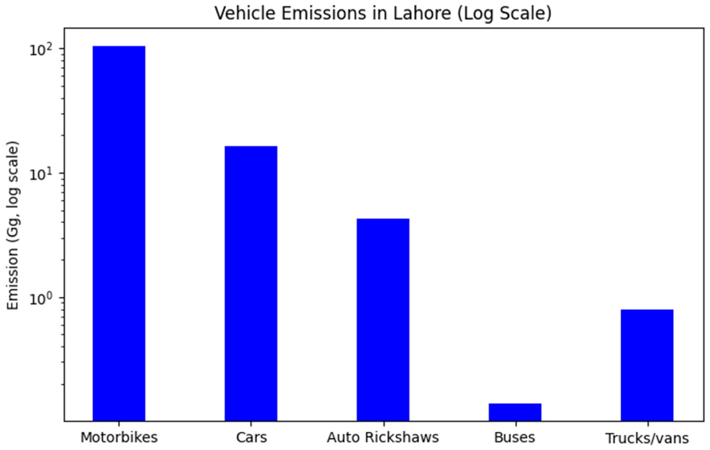
Pie charts in Figure 12 further break down emissions by pollutant type, including NO_x, CO, VOC, and PM, within each sector. Due to the combustion inefficiency of aged cars and two-stroke engines, which are frequently employed in the area, transportation emissions exhibit a clear dominance of PM and CO. The distribution of vehicle-related emissions in Lahore is depicted in Figure 13 in a log-scaled bar chart, which reveals a clear dominance of motorbikes, which significantly contribute the biggest pollution load. Auto-rickshaws, which also have significant emissions because of their frequent use and comparatively inefficient engines, are the second-largest source after cars. Two-wheelers and small personal vehicles are the main sources of emissions in the city’s transportation sector, as the logarithmic scale emphasizes. The larger percentage of NO_x in industrial emissions, as depicted in Figure 11, is indicative of fuel-intensive thermal processes, boiler operations, and manufacturing activities. On the other hand, agricultural emissions exhibit a higher percentage of PM and VOCs, which is consistent with soil-based volatilization processes, residue burning, and open-field biomass combustion. Collectively, this multi-layered representation determines not only the significant contribution of the transport sector but also the pollutant-specific signatures of each emission source, thereby presenting critical insights for designing targeted mitigation strategies.

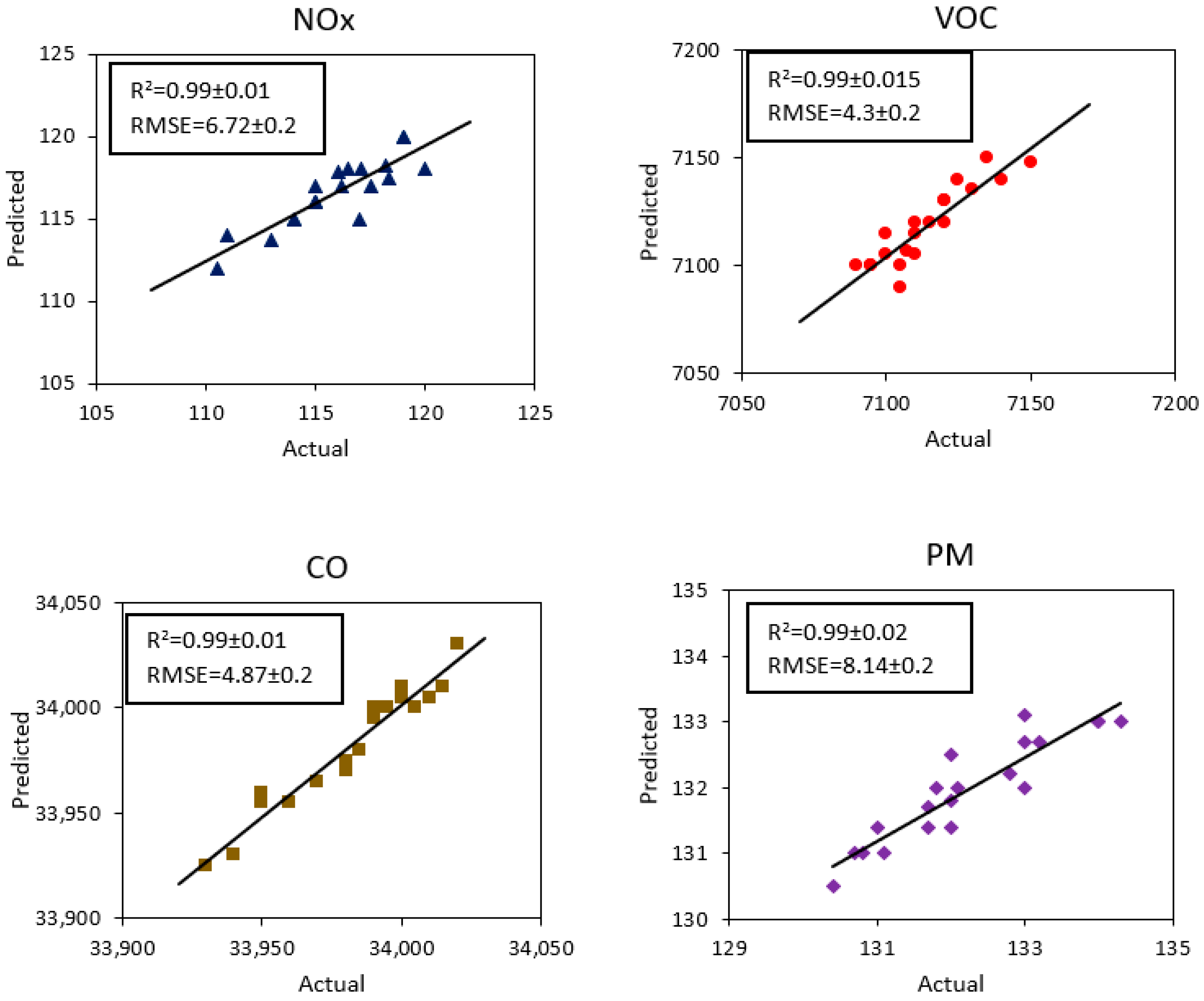
A thorough XGBoost model-performance evaluation for forecasting pollutant concentrations (NO_x, VOCs, CO, and PM) across three key emission sectors, mainly transportation, industry, and agriculture are shown in Figure 14, Figure 15 and Figure 16. Each subplot shows the accuracy and resilience of the used machine learning model by comparing predicted versus real values along with the coefficient of determination (R²) and the Root Mean Square Error (RMSE). For all four pollutants, NO_x, VOCs, CO, and PM, the transport emission results in Figure 14 show extremely dependable forecast performance. Strong agreement between expected and observed values is shown by the scatter plots, which show a close clustering of data points around the 1:1 reference line. The high R² values (0.98–0.99), which verify that the model accounts for nearly all the variability in emissions due to transportation, further support this. The model’s ability to capture the nonlinear features of vehicle emissions is confirmed by the comparably low RMSE values (4.3–8.1), which imply minimal prediction error. These results undervalue the model’s ability to accurately depict fuel combustion patterns, vehicle fleets, and traffic dynamics.

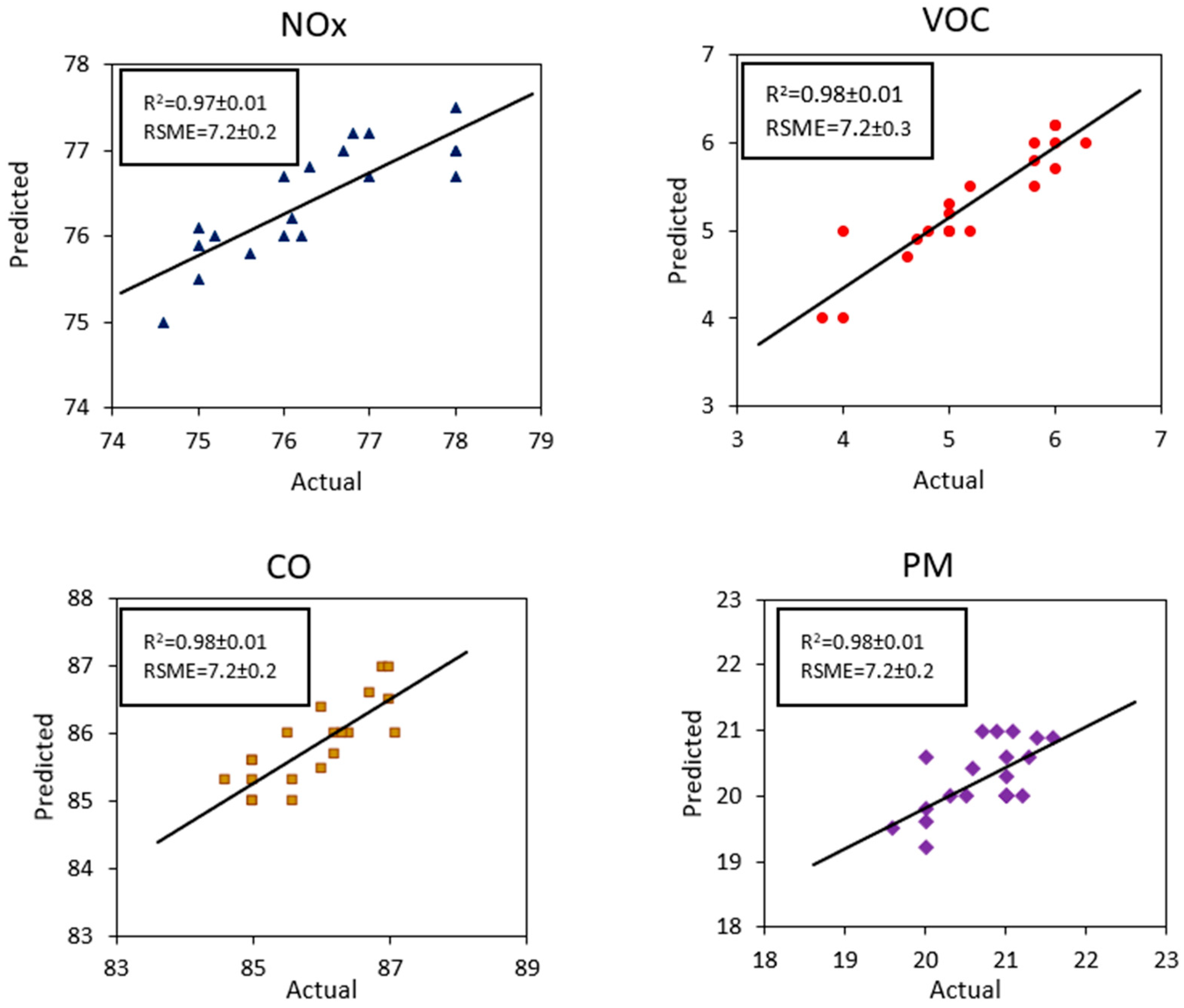
As shown in Figure 15, the model continues to have good predictive performance across NO_x, VOCs, CO, and PM for industrial emissions. The R² values, which have an average of 0.98, demonstrate how effectively the model reflects the emission behavior associated with industrial operations, such as fuel combustion, chemical processing, and manufacturing activities. Despite a slight dispersion when compared to transport emissions, the forecasts are still in good alignment with the 1:1 line, and the RMSE values are still rather low, indicating controlled error margins. This finding demonstrates the model’s ability to control the variability observed in industrial sources, where emission rates routinely vary on operational schedules, process loads, and combustion efficiency. Overall, the results validate the model’s precision in measuring emissions in complex industrial environments.

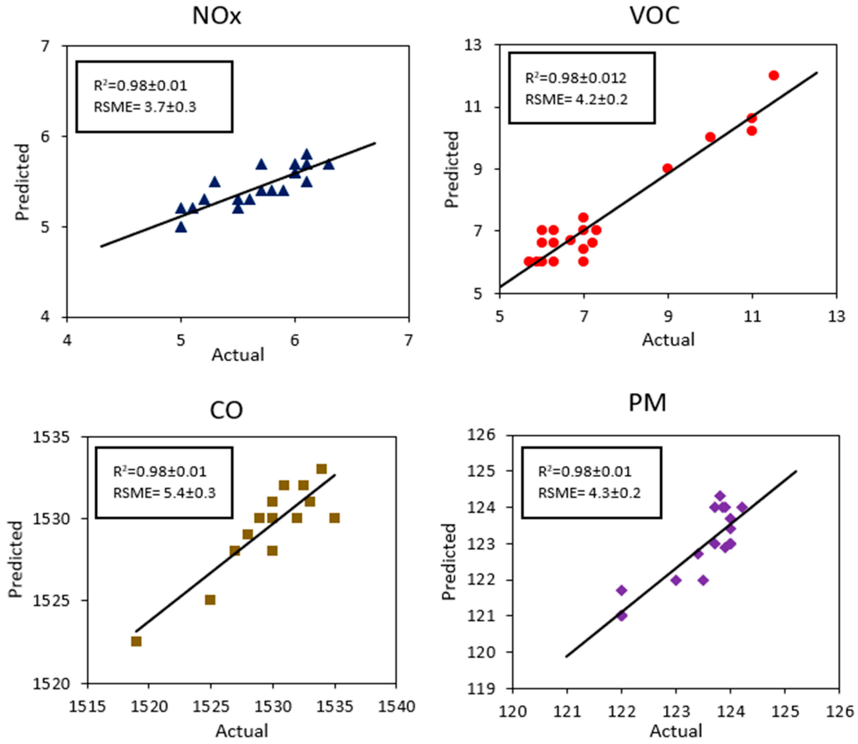
The agricultural emission plots in Figure 16 also exhibit excellent prediction accuracy, with an average R² value of 0.98, demonstrating the strong linear relationship between actual and expected pollution concentrations. The low RMSE values demonstrate how well the model replicates the emission patterns associated with agricultural operations, such as residue burning, soil emissions, and fertilizer-induced volatilization. Despite the seasonal and spatial variability typical of agricultural activities, the model keeps the data points almost perfectly aligned around the ideal prediction line. This consistency demonstrates how well the model accounts for diffuse and intermittent sources of agricultural emissions. Overall, the data suggest that the model is appropriate for accurately calculating the contributions of contaminants resulting from agricultural operations.

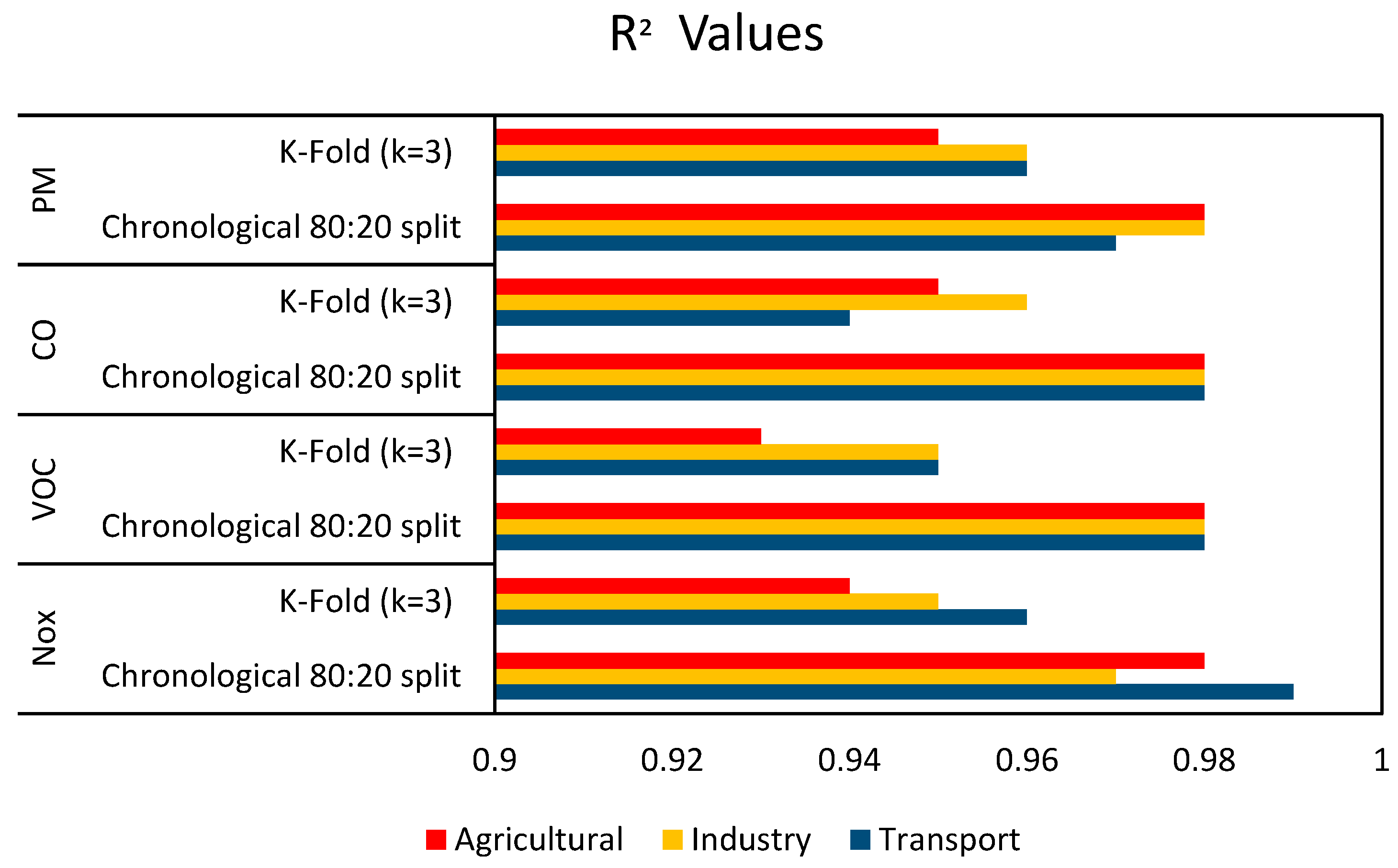
A time-aware validation technique is also used to thoroughly assess predicted performance while maintaining temporal integrity. Time Series k-fold cross-validation (k = 3) is used inside the training set to reduce overfitting issues by iteratively training the model on progressively bigger parts of data and validating it on the following periods. In order to offer reliable estimations of predictive capabilities, the model’s performance is measured using the coefficient of determination (R²) and root mean squared error (RMSE), reporting mean ± standard deviation over folds. This method reduces the possibility of data leakage that comes with traditional random cross-validation and allows an evaluation of model generalizability under practical temporal limitations. The R² value comparison between the chronological split and the k-fold split is displayed in Figure 17, indicating that the k-fold technique is more practical.

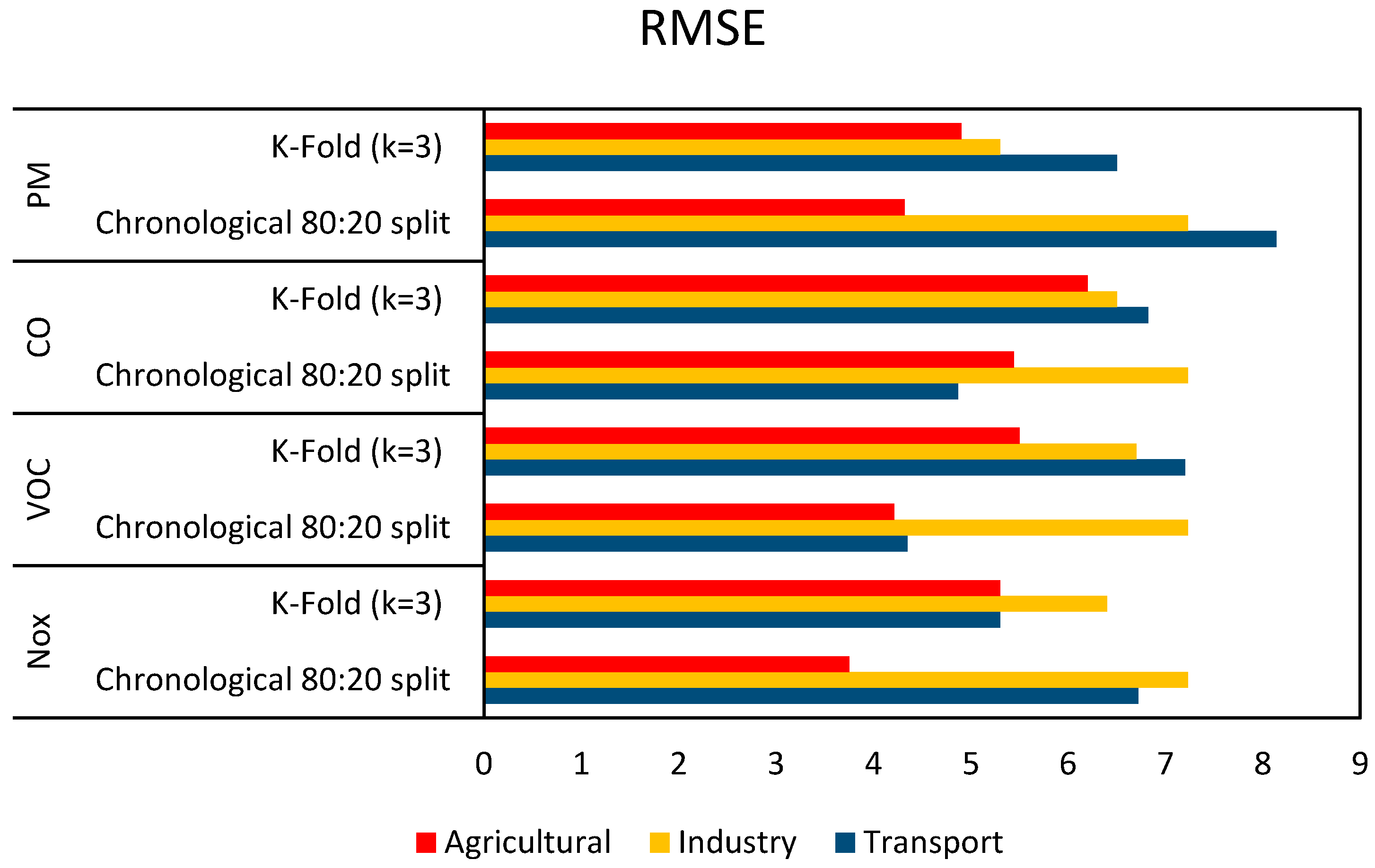
RMSE values for both a chronological split with 80:20 training and test data and k-fold are displayed in Figure 18. Across folds, RMSE values varied from 4.9 to 7.2. This suggests that prediction errors vary somewhat along the folds. The findings show that the machine learning model had moderate prediction accuracy for the 3-month smog dataset and performed consistently across various validation folds.

For both validation procedures, the coefficient of determination (R²) values shows consistently good predictive performance across all three sectors: transportation, industry, and agriculture. When temporal ordering is maintained, R² values for the chronological 80:20 split stay very high, ranging from 0.97 to 0.99 for Transport, 0.97 to 0.98 for Industry, and 0.98 consistently for Agriculture across all model configurations, suggesting outstanding goodness-of-fit. The K-fold (k = 3), on the other hand, produces somewhat lower but still reliable R² values, typically lying between 0.94 and 0.96 for Transport, 0.95 and 0.96 for Industry, and 0.93 and 0.95 for Agriculture. Due to more stringent cross-fold generalization testing, the small decrease shown under K-fold validation is anticipated. Overall, the findings support the models’ strong explanatory power and consistent performance across sectors; chronological validation consistently yields the greatest R² values, indicating the advantage of considering temporal dependencies in the data.

An alternative viewpoint on model accuracy across contaminants and sectors under both validation procedures is provided by the RMSE results. For NO_x, the Transport, Industry, and Agricultural sectors have RMSE values of 6.72, 7.23, and 3.75 for the chronological 80:20 split, respectively, although the K-fold (k = 3) occasionally has equivalent or somewhat larger errors, especially for Agriculture (5.3). RMSE values for VOC under the chronological split range from 4.21 to 7.23, while K-fold validation often yields larger errors (5.5–7.2), showing greater variability when the data are rearranged across folds. For CO, a similar pattern is seen, with chronological RMSE values (4.87–7.23) consistently lower than those derived using K-fold validation (6.2–6.82), indicating improved temporal consistency in forecasts. While K-fold validation produces somewhat lower or equivalent values (4.9–6.5) for some sectors, PM’s RMSE values are still generally higher, with the chronological split yielding errors between 4.32 and 8.14. With very high R² values (≈0.93–0.99) and moderate RMSE levels across all sectors and pollutants, the models show good predictive performance overall, demonstrating significant explanatory power and low prediction error.

4. Mitigation Strategies and Solutions

According to the literature review, industrial and vehicle emissions are the main causes of Lahore’s haze, with particulate matter (PM) and nitrogen oxides (NO_x) being the biggest culprits. The two-phase machine learning framework’s feature importance analysis shows that automobiles are the main source of NO_x and carbon monoxide (CO), while industrial activity significantly raises PM levels. Agricultural activities also have an impact on high PM concentrations, especially in winter when the atmosphere is conducive to pollutant deposition. Strict emission testing, regulatory compliance, and the promotion of cleaner fuels like compressed natural gas (CNG), electric, and hybrid vehicles are examples of targeted automotive interventions. Intelligent traffic signals, dedicated public transportation lanes, odd–even vehicle designs, and traffic management techniques can all help lower emissions. To reduce the dependency on private automobiles, it is advised to expand accessible and efficient public transportation. Cleaner production technologies, such particulate filters and low-NO_x burners, along with strict regulatory compliance and incentive-based emission reduction strategies, can reduce emissions from industrial sources. Pollutant dispersion can be enhanced by urban greening and dust management techniques (road sweeping, water spraying, and construction rules). By planning high-emission activities for windy times, local pollution buildup can be decreased by utilizing natural ventilation. Real-time AQI alerts, the use of masks and interior air purifiers, and citizen education initiatives are all necessary to reduce exposure and encourage behavioral change.

By quantifying sectoral and pollutant-level contributions to AQI, the study’s machine learning methodology makes it possible to prioritize interventions. By addressing nonlinear interactions between emissions and weather, ensemble modeling increases reliability. This methodology emphasizes the broader socioeconomic and health benefits of targeted mitigation by connecting findings to Sustainable Development Goals (SDG 3: Good Health and Well-Being; SDG 11: Sustainable Cities and Communities). To improve policy implementation and refine mitigation strategies, future research should incorporate scenario-based simulations, interactive dashboards, multi-seasonal datasets, high-resolution real-time monitoring, and advanced causal and predictive analyses (e.g., Shapley additive explanation (SHAP), LSTM models). This is because LSTM models are more suited for high-resolution, real-time AQI forecasting since they can learn temporal relationships in sequential data that tree-based models cannot, whereas SHAP captures feature contributions at the individual prediction level. As monitoring infrastructure and datasets become increasingly detailed, it is therefore advised that future projects incorporate these techniques. Although the current study sheds light on the dynamics of smog during the months with the worst pollution, its temporal scope is constrained, and more precise spatial measurements could enhance generalizability. Long-term stability, resilience to distributional changes, and transferability to different areas or longer time horizons are some of the main drawbacks. These factors are recognized as crucial avenues for further investigation to improve the validity and relevance of the results.

5. Conclusions

By combining climatic factors, pollutant profiles, emission inventories, and sophisticated machine learning algorithms, the current study offers a thorough, data-driven evaluation of haze formation in Lahore. Vehicle emissions, industrial activities, and unfavorable weather conditions are the main causes of elevated AQI levels, as demonstrated by the two-phase analytical methodology that assesses total emissions and weather influences before doing pollutant-specific toxicity analysis. Excellent predictive power was demonstrated by both Random Forest and XGBoost models. CO, NO_x, VOCs, and particulate matter were found to be the most important factors influencing the intensity of smog using feature-importance analysis. With R² of 0.93–0.99 and RMSE of 4.3–8.4, XGBoost successfully forecasted all emissions categories. By connecting emission dynamics with public health hazards, declining visibility, and pertinent Sustainable Development Goals (SDG 3 and SDG 11), our validated results show accurate short-term AQI predictions and support practical recommendations for emission reduction measures.

To account for deeper spatial variability in smog dynamics, future work will enhance the suggested framework by extending the analysis to additional cities, even though time-aware cross-validation enabled robust temporal validation in the current study. Evaluation of the model’s generalizability across various urban contexts, emission profiles, and climatic circumstances will be made possible by this development. Key limitations, including long-term stability, robustness to distributional shifts, and transferability across regions and extended time horizons, are therefore identified as important directions for future research, aimed at strengthening the reliability and scalability of the proposed predictive approach.

References

1. IQAir. World Air Quality Report; IQAir: Steinach, Switzerland, 2024. [Google Scholar]
2. Abhranil, B.; Tapoban, B.; Rabin, D.; Abu Md Ashif, I.; Bikash, D.; Waikhom Somraj, S. Assessing AQI of air pollution crisis 2024 in Delhi: Its health risks and nationwide impact. Discov. Atmos. 2025, 3, 13. [Google Scholar] [CrossRef] [Scilit]
3. Abdul, R.; Muhammad Mubashar, Z.; Laviza Tuz, Z.; Fariha, Q.; Fei, Q.; Muhammad Haseeb, U.; Saadia, S.; Ghulam, R.; Xuefei, J. Smog: Lahore needs global attention to fix it. Environ. Chall. 2024, 16, 100999. [Google Scholar] [CrossRef] [Scilit]
4. Ying, Z.; Song Xi, C.; Le, B. Air pollution estimation under air stagnation—A case study of Beijing. Environmetrics 2023, 34, e2819. [Google Scholar] [CrossRef] [Scilit]
5. Zheng, X.; Xuerui, Y.; Hongming, G.; Jialiang, H.; Tongguang, Z.; Jianian, C.; Xukang, P.; Guangli, X.; Wei, Z.; Mingyue, L. Characterization and sources of volatile organic compounds (VOCs) during 2022 summer ozone pollution control in Shanghai, China. Atmos. Environ. 2024, 327, 120464. [Google Scholar] [CrossRef] [Scilit]
6. Amir, G.; Davoud, G. Identifying the Causes of Air Pollution in the Tehran Metropolis-Iran and Policy Recommendations for Sustainability. Aerosol Sci. Eng. 2025, 9, 1–15. [Google Scholar] [CrossRef] [Scilit]
7. Rabia, M.; Muhammad Shehzaib, A.; Muhammad, I.-u.-d.; Suhaib, M.; Muhammad Naveed, A.; Bilal, A.; Muhammad Fahim, K. Solving the mysteries of Lahore smog: The fifth season in the country. Front. Sustain. Cities 2024, 5, 1314426. [Google Scholar] [CrossRef] [Scilit]
8. Prakash Chand, K. Air Pollution in Delhi: Causes and Consequences. In Combating Air Pollution; Springer: Cham, Germany, 2024; pp. 61–75. [Google Scholar] [CrossRef] [Scilit]
9. Kinjal, B.; Vishal, S. Sustainable Solutions for Delhi’s Air Pollution: A Data Driven Approach. In Proceedings of the 1st International Conference on Advanced Materials for Sustainable Innovation, New Delhi, India, 28–30 August 2024; pp. 143–157. [Google Scholar]
10. Ashima, S.; Renu, M. Rising Extreme Event of Smog in Northern India: Problems and Challenges. In Extremes in Atmospheric Processes and Phenomenon: Assessment, Impacts and Mitigation; Springer: Singapore, 2022; pp. 205–236. [Google Scholar] [CrossRef] [Scilit]
11. Muhammad, N.-u.-M.; Masooma, Z.; Muhammad, J. Exploring mitigation strategies for smog crisis in Lahore: A review for environmental health, and policy implications. Environ. Monit. Assess. 2024, 196, 1296. [Google Scholar] [CrossRef] [Scilit] [PubMed]
12. Aiman, F.; Derk, B. Assessment of Brick Kilns’ contribution to the air pollution of Lahore using air quality dispersion modeling. Environ. Monit. Assess. 2025, 197, 318. [Google Scholar] [CrossRef] [Scilit] [PubMed]
13. Uzma, N.; Muhammad, I. Smog diplomacy: Strengthening Pakistan-India cooperation for transboundary air pollution. J. Clim. Community Dev. 2025, 4, 55–65. [Google Scholar]
14. Muhammad, Z. Spatiotemporal analysis of tropospheric nitrogen dioxide hotspot over Lahore Division in Pakistan. Discov. Environ. 2025, 3, 113. [Google Scholar] [CrossRef] [Scilit]
15. IQAir. Live Most Polluted Major City Ranking. Available online: https://www.iqair.com/us/world-air-quality-ranking (accessed on 23 October 2025).
16. Environmental Protection Agency, Government of Punjab, Pakistan; IQAir. Lahore Air Quality Map. Available online: https://www.iqair.com/au/air-quality-map/pakistan/punjab/lahore (accessed on 17 November 2025).
17. District Health Information System. Disease Wise Analytics. Available online: https://dhispb.com/ (accessed on 17 November 2025).
18. Rachna, A.; Girija, J.; Sneh, A.; Marimuthu, P. Assessing Respiratory Morbidity Through Pollution Status and Meteorological Conditions for Delhi. Environ. Monit. Assess. 2006, 114, 489–504. [Google Scholar] [CrossRef] [Scilit] [PubMed]
19. Mario, J.M.; Luisa, T.M. Megacities and Atmospheric Pollution. J. Air Waste Manag. Assoc. 2004, 54, 644–680. [Google Scholar] [CrossRef] [Scilit] [PubMed]
20. The Urban Unit Government Office. The Urban Unit. Available online: https://urbanunit.gov.pk/ (accessed on 17 November 2025).
21. Ghosh, S.; Sinha, D. Indian perspective of PM2.5 attributed human health hazards during 2010–2025. Air Qual. Atmos. Health 2025, 18, 2765–2804. [Google Scholar] [CrossRef] [Scilit]
22. Kumar, P.; Singh, S.; Tyagi, E.; Pathak, V.M.; Gupta, S.; Singh, R. Role of Gases, VOC, PM2.5, and PM10 in Biological Contamination in Indoor Areas. In Airborne Biocontaminants and Their Impact on Human Health; Wiley: Hoboken, NJ, USA, 2024; pp. 89–107, Chapter 5. [Google Scholar]
23. Shazia, I.; Iqra, Q.; Rabia, S.; Muhammad Saleem, P.; Matthias, S.; Elke, H. Impact of Air Pollution and Smog on Human Health in Pakistan: A Systematic Review. Environments 2025, 12, 46. [Google Scholar] [CrossRef] [Scilit]
24. Shima, M. Epidemiological studies on the health impact of air pollution in Japan: Their contribution to the improvement of ambient air quality. Environ. Health Prev. Med. 2025, 30, 30. [Google Scholar] [CrossRef] [Scilit]
25. Emmanuel, O.; Aria, J.; Jose, D.; Diego, C. Environmental Impacts of Airborne Contaminants. 2025. Available online: https://www.researchgate.net/publication/387831501_Environmental_Impacts_of_Airborne_Contaminants (accessed on 17 November 2025).
26. Hussain, A.; Abbas, M.; Kabir, M. Smog Pollution in Lahore, Pakistan: A Review of the Causes, Effects, and Mitigation Strategies. Preprints 2025. [Google Scholar] [CrossRef] [Scilit]
27. Jagathesan, T. Exploring the spatial and inter-temporal spill-over effects of Air Pollution in Chennai City—A Study. Cent. Dev. Econ. Stud. 2022, 9, 32–42. [Google Scholar] [CrossRef] [Scilit]
28. Çelik, M.Ö.; Orhan, O.; Kurt, M.A. Drivers and Impacts of Climate Change: Comprehensive Review of Natural and Anthropogenic Forcing with GCM-Based Projections. Geomat. Environ. Eng. 2025, 19, 71–101. [Google Scholar] [CrossRef] [Scilit]
29. Cheng, S.; Zheng, Y.; Li, G.; Gao, J.; Li, R.; Yue, T. Research progress on phase change absorbents for CO2 capture in industrial flue gas: Principles and application prospects. Sep. Purif. Technol. 2025, 354, 129296. [Google Scholar] [CrossRef] [Scilit]
30. To‘lqinjonovna, A.F. Smog is a Serious Risk to Human Health. Web Med. J. Med. Pract. Nurs. 2025, 3, 157–160. [Google Scholar]
31. Alighiri, D.; Widodo, N.B.; Abdullah, R.A.; Firnanda, I.P.; Drastisianti, A. Risk analysis of air quality for parameters NO2, SO2, NH3, and Ox from the area around fertilizer industries in Indonesia. J. Nat. Sci. Math. Res. 2025, 11, 29–46. [Google Scholar] [CrossRef] [Scilit]
32. Malakan, W.; Kc, S.; Jalearnkittiwut, T.; Samniang, W. Indoor Air Pollution of Volatile Organic Compounds (VOCs) in Hospitals in Thailand: Review of Current Practices, Challenges, and Recommendations. Atmosphere 2025, 16, 1135. [Google Scholar] [CrossRef] [Scilit]
33. Héluain, V.; Molinier, L.; Mazières, J. Air pollution and lung cancer: A comprehensive review. J. Epidemiol. Popul. Health 2025, 73, 203152. [Google Scholar] [CrossRef] [Scilit]
34. Faruqui, N.; Orell, S.; Dondi, C.; Leni, Z.; Kalbermatter, D.M.; Gefors, L.; Rissler, J.; Vasilatou, K.; Mudway, I.S.; Kåredal, M. Differential Cytotoxicity and Inflammatory Responses to Particulate Matter Components in Airway Structural Cells. Int. J. Mol. Sci. 2025, 26, 830. [Google Scholar] [CrossRef] [Scilit] [PubMed]
35. Qiao, S.; Guo, Q.; He, Z.; Feng, G.; Wang, Z.; Li, X. Spatiotemporal Trends and Drivers of PM2. 5 Concentrations in Shandong Province from 2014 to 2023 Under Socioeconomic Transition. Toxics 2025, 13, 978. [Google Scholar] [CrossRef] [Scilit] [PubMed]
36. Okafor, V.N.; Okoye, N.H.; Omokpariola, D.O.; Ume, C.B.; Ujam, O.T. Risk assessments of polycyclic aromatic hydrocarbons in the surface sediments of drinking water sources in Ifite Ogwari, South-East Nigeria. Soil Sediment Contam. Int. J. 2025, 34, 187–206. [Google Scholar] [CrossRef] [Scilit]
37. Arghiropol, D.; Rusu, T.; Moldovan, M.; Paltinean, G.-A.; Silaghi-Dumitrescu, L.; Sarosi, C.; Petean, I. Petroleum Hydrocarbon Pollution and Sustainable Uses of Indigene Absorbents for Spill Removal from the Environment—A Review. Sustainability 2025, 17, 8018. [Google Scholar] [CrossRef] [Scilit]
38. Vongelis, P.; Koulouris, N.G.; Bakakos, P.; Rovina, N. Air Pollution and Effects of Tropospheric Ozone (O3) on Public Health. Int. J. Environ. Res. Public Health 2025, 22, 709. [Google Scholar] [CrossRef] [Scilit]
39. Ioannou, A.; Papadopoulos, E.; Qaderi, M. The Impact of Air Pollution on Chronic Respiratory Diseases. Int. J. Med. Appl. Health Sci. 2025, 1, 14–20. [Google Scholar]
40. Shrivastav, M.; Rabani, M.S.; Pathak, A.; Sharma, J.K.; Gupta, C.; Gupta, M.K. Consequences of Toxic Heavy Metals. In Global Perspectives of Toxic Metals in Bio Environs: Volume 1: Environmental Impact, Ecotoxicology, Health Concerns, and Modelling; Springer: Cham, Germany, 2025; p. 127. [Google Scholar]
41. Jyothi, N.R. Mapping Our Metallic Mess: Advanced Modeling for Heavy Metal Dispersion. In Global Perspectives of Toxic Metals in Bio Environs: Volume 1: Environmental Impact, Ecotoxicology, Health Concerns, and Modelling; Springer: Cham, Germany, 2025; p. 51. [Google Scholar]
42. Siddiqui, S.A.; Neda, F.; Anwar, A. Smart air pollution monitoring system with smog prediction model using machine learning. Int. J. Adv. Comput. Sci. Appl. 2021, 12, 401–409. [Google Scholar] [CrossRef] [Scilit]
43. Pervaiz, Z.; Rehman, S.; Ayesha, K.; Muhammad, R. Predictive Analysis of Smog Exposure and Its Impact on Human Health Outcomes. J. Comput. Biomed. Inform. 2025, 9, 1–10. [Google Scholar]
44. Muhammad Fahad, M.; Muhammad Salman, Q.; Athar, W.; Ubaid, U.; Mardeni, B.R.; Ahmed, S. Predicting Air Quality in Pakistan with a Focus on Smog Formation: A Machine Learning Approach. In Proceedings of the International Conference on Engineering and Emerging Technologies (ICEET), Dubai, United Arab Emirates, 27–28 December 2024. [Google Scholar]
45. Sandhya, S.; Arun, S. Machine learning approach to PM2.5 forecasting and health risk assessment during stubble burning period in Delhi. Aerosol Sci. Technol. 2025, 59, 1385–1404. [Google Scholar] [CrossRef] [Scilit]
46. Akila, R.; Balasakthipriyan, M. Stubble Burning and Its Impact in Delhi’s Air Pollution of india: Predictive Approach Using Machine Learning. Appl. Ecol. Environ. Res. 2025, 23, 7935–7956. [Google Scholar] [CrossRef] [Scilit]
47. Zhiyuan, L.; Steve Hung-Lam, Y.; Kin-Fai, H. High temporal resolution prediction of street-level PM2.5 and NOx concentrations using machine learning approach. J. Clean. Prod. 2020, 268, 121975. [Google Scholar] [CrossRef] [Scilit]
48. Thomas, M.T.L.; Jianxiu, C.; Altaf Hossain, M.; Tonni Agustiono, K.; Steven Soon-Kai, K. Evaluation of Machine Learning Models in Air Pollution Prediction for a Case Study of Macau as an Effort to Comply with UN Sustainable Development Goals. Sustainability 2024, 16, 7477. [Google Scholar] [CrossRef] [Scilit]
49. Yanchuan, S.; Wei, Z.; Riyang, L.; Jianxun, Y.; Miaomiao, L.; Wen, F.; Litiao, H.; Matthew, A.; Jun, B.; Zongwei, M. Estimation of daily NO2 with explainable machine learning model in China, 2007–2020. Atmos. Environ. 2023, 314, 120111. [Google Scholar] [CrossRef] [Scilit]
50. Komal, Z.; Sana, S.; Salman, T. Prediction of aerosol optical depth over Pakistan using novel hybrid machine learning model. Acta Geophys. 2023, 71, 2009–2029. [Google Scholar] [CrossRef] [Scilit]
51. Abu Reza, M.d.; Towfiqul, I.; Mohammed Al, A.; Javed, M.; Subodh Chandra, P.; Rabin, C.; Abdul, F.M.d.; Bonosri, G.; Most Kulsuma Akther, K.; Aminul, I.M.d.; et al. Estimating ground-level PM2.5 using subset regression model and machine learning algorithms in Asian megacity, Dhaka, Bangladesh. Air Qual. Atmos. Health 2023, 16, 1117–1139. [Google Scholar] [CrossRef] [Scilit]
52. Alibek, I.; Nurtugan, R.; Aizhan, A. Predicting particulate matter (PM2.5) air pollution levels in Almaty city using machine learning techniques. Model. Earth Syst. Environ. 2025, 11, 236. [Google Scholar] [CrossRef] [Scilit]
53. Gokulan, R.; Gasim, H.; Karthick, K.; Avinash, A.; Christian, S. Air quality prediction by machine learning models: A predictive study on the indian coastal city of Visakhapatnam. Chemosphere 2023, 338, 139518. [Google Scholar] [CrossRef] [Scilit] [PubMed]
54. AccuWeather, Lahore, Pakistan. Available online: https://www.accuweather.com/en/pk/lahore/260622/weather-forecast/260622 (accessed on 17 November 2025).
55. Sevtap, T. Machine learning-based forecasting of air quality index under long-term environmental patterns: A comparative approach with XGBoost, LightGBM, and SVM. PLoS ONE 2025, 20, e0334252. [Google Scholar] [CrossRef] [Scilit]
56. Rudy, W.; Mauridhi Hery, P.; Wiwik, A. Enhancing Predictive Emissions Monitoring Performance: Data Preprocessing for XGBoost-Based Model Algorithm. In Proceedings of the 17th International Conference on Knowledge and Smart Technology, Bangkok, Thailand, 26 February–1 March 2025. [Google Scholar]
57. Stefan, W.; Marcel, L.; Sebastian, S.; Raphael, F.; Tobias, S. Hourly Particulate Matter (PM10) Concentration Forecast in Germany Using Extreme Gradient Boosting. Atmosphere 2024, 15, 525. [Google Scholar] [CrossRef] [Scilit]
Figure 1. Most polluted cities in terms of AQI as per 10 December 2025 statistics.
Gases 06 00010 g001
Figure 2. AQI levels in different parts of Lahore on 24 November 2025 [16].
Gases 06 00010 g002
Figure 3. Diseases reported in Lahore credited to air pollution [17].
Gases 06 00010 g003
Figure 4. Disease pattern reported in the smog season in Lahore during 2022.
Gases 06 00010 g004
Figure 5. Smog formation process diagram.
Gases 06 00010 g005
Figure 6. Flowchart of the Two-Phase Methodology for analyzing smog formation in Lahore.
Gases 06 00010 g006
Figure 7. Mobile Station deployed in Lahore to monitor air quality.
Gases 06 00010 g007
Figure 8. Comparison of XGBoost and Random Forest Model for predicting AQI.
Gases 06 00010 g008
Figure 9. Variable Importance Coefficients for AQI Prediction Using Random Forest Model.
Gases 06 00010 g009
Figure 10. Variable Importance Coefficients for AQI Prediction Using XGBoost Model.
Gases 06 00010 g010
Figure 11. Sector-wise breakdown of total annual emissions (Tons) in Lahore.
Gases 06 00010 g011
Figure 12. Emissions in Tons within each sector of the four major pollutant types: NOx, CO, VOC and PM.
Gases 06 00010 g012
Figure 13. Vehicle emissions in Lahore are categorized by transport type.
Gases 06 00010 g013
Figure 14. Model predictions for Transport Emissions in Tons.
Gases 06 00010 g014
Figure 15. Model predictions for Industry Emissions in Tons.
Gases 06 00010 g015
Figure 16. Model predictions for Agricultural Emissions in Tons.
Gases 06 00010 g016
Figure 17. R2 values for model evaluation for chronological split versus k-split.
Gases 06 00010 g017
Figure 18. RMSE values model evaluation for chronological split versus k-split.
Gases 06 00010 g018