Solar Irradiance Forecasting in Data-Sparse Tropical Regions Using a Novel Spatial Site-Adapted WRF–LSTM Hybrid Approach

Abstract

Accurate solar irradiance forecasting in data-sparse tropical regions remains challenging due to complex terrain, rapid convective cloud formation, and limited ground-based observations. This study introduces a novel hybrid forecasting framework that integrates the Weather Research and Forecasting (WRF) model (10 km) with station-based Long Short-Term Memory (LSTM) bias correction, complemented by three innovative spatial site-adaptation strategies to produce spatially coherent short-term irradiance fields. The hybrid system leverages hourly Global Horizontal Irradiance (GHI) data from eight BMKG stations (2023) alongside GK2A satellite cloud information to dynamically correct WRF forecast biases, capturing nonlinear cloud–irradiance interactions that standard Numerical Weather Prediction (NWP) models fail to resolve. Results indicate that the hybrid WRF–LSTM system reduces 1–3-day root mean square error (RMSE) by 120–127 W/m² and relative RMSE (rRMSE) by 26%, while lowering relative mean bias error (rMBE) from 31–36% (raw WRF) to 2.5–4.1%, with the largest improvements observed in regions exhibiting initially high WRF errors. Among the spatial adaptation methods, the average-based scheme minimizes RMSE but exhibits weak spatial coherence; the distance-weighted scheme achieves the strongest spatial consistency with regional reanalysis (R² = 0.37) with minimal bias; and the elevation-based scheme ensures full-domain coverage with moderate skill. This study demonstrates that the integration of dynamical NWP modeling with LSTM-based bias correction and tailored spatial transfer strategies provides a robust, scalable approach for short-term solar irradiance forecasting and resource mapping in tropical environments. The proposed framework offers practical implications for PV power forecasting, grid management, and renewable energy planning in regions where observational data are sparse and the terrain is highly heterogeneous.

1. Introduction

Global warming, reflected by a persistent rise in Earth’s surface temperature, remains one of the most critical challenges facing humanity. Since the pre-industrial period (1850–1900), global mean temperatures have increased by approximately 1.1 °C as a direct result of greenhouse gas accumulation in the atmosphere. Furthermore, projections indicate a possible rise of 2–4 °C by the end of the 21st century without significant mitigation strategies to alter current emission trajectories [1]. Despite global initiatives such as the Paris Agreement aiming to cap this temperature increase, the continued burning of fossil fuels continues to drive warming. Consequently, this ongoing shift produces far-reaching consequences for climate systems, ecosystems, and human well-being, including sea-level rise and the increased frequency of extreme weather events [2].

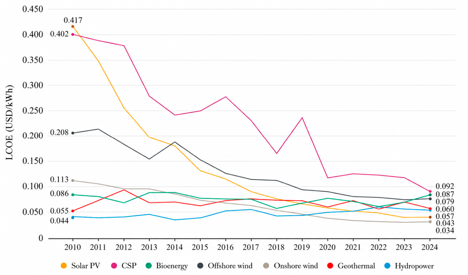
Solar energy has therefore emerged as a key mitigation instrument to reduce global reliance on carbon-intensive power generation. Its natural abundance, long-term sustainability, and rapidly declining manufacturing costs have significantly strengthened the role of solar photovoltaic (PV) systems in the architecture of future low-carbon power grids. Over the past decade, advancements in material science and economies of scale have caused the levelized cost of PV electricity to drop from USD 0.417/kWh in 2010 to roughly USD 0.043/kWh in 2024. Similar reductions have been documented for concentrated solar power technologies as supply chains mature and installation efficiencies improve [3]. These trends underscore the increasingly competitive economics of large- and small-scale PV deployment, as shown in Figure 1.

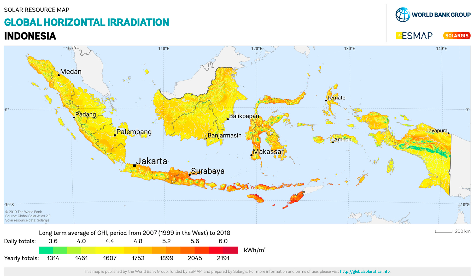
Located along the equator, Indonesia benefits from consistent year-round daylight hours, resulting in a national average solar irradiation of 4.62 kWh/m²/day [4,5]. Regional atmospheric dynamics create distinct localized peaks; for example, southern areas such as the Nusa Tenggara Islands experience fewer monsoonal disruptions and achieve irradiation levels between 5.0 and 5.6 kWh/m²/day (Figure 2) [4,5]. National energy assessments quantify the country’s theoretical solar potential at 3294 GW for broader utility-scale developments [6]. Concurrently, decentralized rooftop PV systems across urban and residential sectors could contribute an additional 194 to 655 GW directly to the grid [7]. However, the practical exploitation of this generation capacity is constrained by severe regional variations in cloud cover, aerosol distribution, and highly dynamic tropical convective weather patterns across the archipelago [8].

West Java represents a critical hub for renewable energy development due to its dense population, rising electricity demand, and underutilized solar assets estimated at a strategic potential of 155.5 GWp [9,10]. Serving roughly 17 million customers—approximately 19% of Indonesia’s national total—the region’s massive load profile underscores the vital importance of optimizing its grid infrastructure [6,11]. Geographically, however, the province is characterized by a complex topographical layout featuring mountainous interiors and extensive coastlines that drive active land–sea atmospheric interactions. These localized terrain features interact with broader regional weather systems to introduce substantial operational uncertainties for photovoltaic (PV) applications. Specifically, rapid transitions in cloud cover, pronounced monsoonal shifts, and convective storm developments sharply reduce surface irradiance, triggering abrupt PV output fluctuations. Consequently, these sudden generation deficits induce severe grid-management challenges, necessitating reliable short-term forecasting solutions to counter weather-driven variability and maintain stable power delivery [12,13,14].

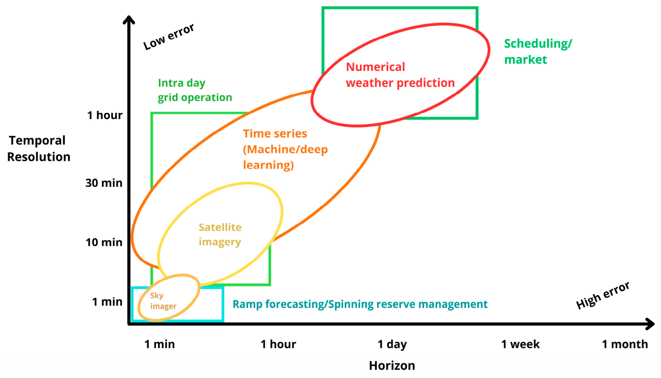
To effectively manage grid stability amidst continuous atmospheric variability, utility operators require highly precise solar irradiance forecasting systems. Currently, in general, there are six primary classifications of forecasting methodologies: time-series statistical models, machine learning (ML) and deep learning (DL) frameworks, numerical weather prediction (NWP) systems, satellite-derived models, ground-based sky imagers, and hybrid architectures that integrate multiple techniques [15]. Each individual category is optimized for specific temporal and spatial operational requirements. For immediate grid balancing, localized sky imagers generate precise minute-scale nowcasts, while satellite observations and time-series algorithms perform optimally for predicting minute-to-hour horizons across broader regional footprints. Conversely, NWP frameworks such as the Weather Research and Forecasting (WRF) model are structurally designed for day-ahead to multi-day scheduling, yet they frequently produce larger uncertainty margins when simulating rapid cloud formation in convective tropical environments [16]. A comprehensive comparative summary of these approaches is presented in Figure 3, adapted from [16], which maps out the distinct temporal resolutions and forecasting horizons that fundamentally motivate the hybrid NWP–DL configuration utilized in this study.

Deep learning models—particularly Long Short-Term Memory (LSTM) networks—are widely utilized for short-term solar irradiance forecasting due to their structural capacity to process temporal dependencies within meteorological time series [17,18]. By utilizing internal gating mechanisms to filter and retain relevant historical data, these algorithms effectively capture non-linear atmospheric patterns without requiring explicit physical equations [17,18]. For example, LSTM approaches have achieved one-day-ahead Root Mean Square Error (RMSE) values of 41–46 W/m² in urban areas of the United States, alongside relative RMSEs of 11–12% across arid regions such as Morocco and parts of Europe [17,18,19]. However, the accuracy of these data-driven models frequently degrades in tropical climates. In these specific environments, highly variable cloud dynamics, rapid convective storm formation, and fluctuating aerosol loading introduce large stochastic components that standard sequential models struggle to resolve [20].

Standalone ML frameworks offer robust temporal pattern recognition but require extensive, high-quality historical observations for training. This data dependency poses a significant hurdle, as comprehensive ground-based meteorological datasets remain scarce across many developing regions. In contrast, NWP systems, such as the WRF model, provide a valuable alternative by delivering spatially continuous, multi-day forecasts that simulate atmospheric dynamics, multi-scale cloud evolution, and complex radiative transfer mechanisms. A primary benefit of these meteorological models is their operational flexibility, which allows them to replicate both present and future climatic conditions across a wide range of spatial and temporal coverages. Furthermore, augmented configurations such as WRF-Solar offer a distinct advantage by generating high-frequency time series of all solar irradiance components, which is particularly critical for modeling photovoltaic power output ramps caused by abrupt changes in surface radiation [21]. Nonetheless, these physical WRF forecasts often struggle in highly dynamic tropical environments, commonly exhibiting substantial sub-daily inaccuracies with RMSE values frequently recorded between 112.45 and 320 W/m² [22,23,24,25,26,27]. These persistent errors are largely due to the inherent limitations of physical parameterization schemes in resolving rapid convective processes, combined with the spatial smoothing effects imposed by coarse operational grid spacing [26,27].

To address the limitations of standalone models, hybrid forecasting systems integrate NWP outputs with machine learning/statistical-based bias correction algorithms. This dual architecture leverages the physical spatial resolution of NWP alongside the temporal pattern recognition capabilities of machine learning to reduce RMSE and systematic bias across diverse climate zones [28,29,30,31,32]. The recent literature demonstrates the efficacy of this hybrid methodology across various geographic and climatic contexts. In arid climates, coupling the WRF model with Gaussian Process Regression reduces RMSE by up to 70.2% compared to standalone numerical predictions [28]. This approach has also been validated in East Asia; integrating high-resolution WRF outputs with a clearness index-based Kalman filter improved clear-sky forecasting accuracy by 42.2% and 26.8% in RMSE across different regional sites [29]. In Toledo, Spain, integrating WRF variables with a Grouping Genetic Algorithm and an Extreme Learning Machine yielded an RMSE of 75.56 W/m² [30]. Furthermore, in tropical island environments, the integration of WRF with LSTM networks proves effective. In Timor-Leste, implementations of these hybrid WRF-LSTM frameworks have maintained relative RMSE (rRMSE) values below 20%, while a comparable spatio-temporal network configuration in Reunion Island yielded an hourly rRMSE of 14.05% [31,32].

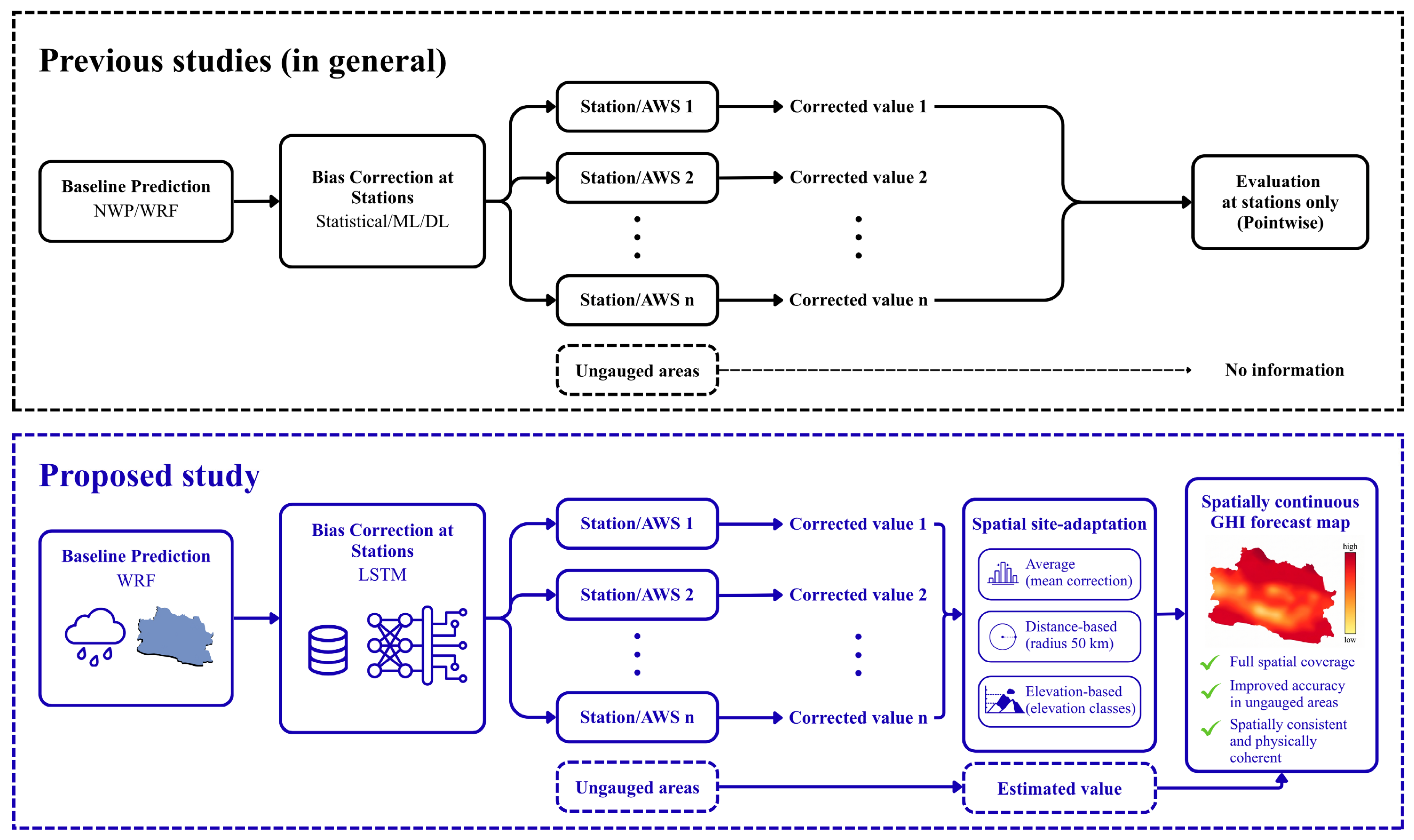
Despite these algorithmic advancements and temporal error reductions, current hybrid architectures remain restricted in their spatial application. The corrections applied by deep learning or statistical filters are anchored to the geographic coordinates of the available ground observation sites. As illustrated in the top panel of Figure 4, these conventional forecasting frameworks, whether standalone or hybrid, evaluate performance exclusively at the point level. This lack of spatial extrapolation leaves the surrounding unmonitored grid cells uncorrected, presenting a barrier to generating accurate, continuous regional solar resource maps in data-sparse environments.

Separately, in the realm of long-term PV resource assessment, researchers frequently incorporate site-adaptation procedures to reconcile modeled or satellite-derived estimations with empirical ground measurements. Frameworks such as SiteAdapt implement regression equations and empirical distribution matching to mitigate random variance and systematic deviations within historical data [33,34]. As detailed in

Table 1. Summary of previous site-adaptation irradiance studies.

Author(s)	Objective	Methods	Data Sources	Forecast Horizon
Polo et al. (2016) [33] & Fernández-Peruchena et al. (2020) [34]	To establish and validate the traditional statistical “SiteAdapt” framework for resource assessment.	Linear Regression & Empirical Quantile Mapping (eQM)	Long-term modeled or satellite irradiance data & point-level ground measurements.	Historical correction (No future forecasting)
Zainali et al. (2024) [35]	To test various machine learning algorithms as a replacement for traditional statistical site adaptation.	9 traditional Machine Learning algorithms (operating strictly pointwise).	Gridded regional irradiance product (STRÅNG) & high-latitude ground stations.	Historical correction
Dhata et al. (2022) [36]	To compare regressive versus distribution matching techniques for correcting satellite data.	Linear Regression, Quantile Mapping, & Empirical Distribution Matching.	Satellite-derived irradiance (COMS Level-1B) & single-station ground data.	Historical correction (2014–2019)
Narvaez et al. (2021) [37]	To utilize machine learning algorithms for site-adaptation of satellite data and deep learning for subsequent solar radiation forecasting.	Random Forest regression for site-adaptation & Encoder-Decoder LSTM/GRU networks	Satellite-derived data (NSRDB) & in situ ground measurements (IDEAM)	Daily (24 h) and weekly (168 h).
Juliansyah et al. (Proposed Study)	To develop a spatially continuous, dual-tier forecasting and mapping framework for data-sparse tropical regions.	Dual-Tier WRF-LSTM Hybrid + 3 Spatial Site-Adaptation Schemes (Average, Distance, Elevation).	NWP (WRF), GK2A satellite, GFS forcing, & 8 AWS ground stations.	Hourly, 1 to 3 days ahead

, subsequent research has diversified the methodological approaches and objectives within this domain. Recent studies evaluate an array of machine learning algorithms to replace traditional statistics [35] or compare complex regression techniques against empirical distribution models to optimize satellite data correction [36]. Further bridging the gap between historical data correction and prediction, advanced frameworks have recently applied machine learning algorithms such as Random Forests for site-adaptation, creating an improved meteorological database that directly trains sequence-to-sequence deep learning forecasting networks [37]. However, despite this methodological evolution and validation across distinct geographic contexts, from high-latitude regions [35] to temperate zones [36], these conventional site-adaptation methodologies operate strictly at the discrete point level. They lack the geospatial mechanisms required to extrapolate localized corrections across unmonitored grid cells. Furthermore, existing frameworks remain restricted to correcting retrospective datasets rather than generating operational forecasts. A comprehensive comparative summary of these site-adaptation studies, highlighting the specific spatial and temporal limitations that necessitate this study’s proposed configuration, is presented in Table 1.

Motivated by these methodological gaps, specifically the restriction of traditional forecasting and site-adaptation to isolated point locations and historical data, this study develops the spatially continuous framework depicted in the bottom panel of Figure 4. This dual-tier architecture integrates a hybrid WRF–LSTM temporal forecasting system with three spatial site-adaptation strategies to extrapolate corrected irradiance estimates across unmonitored areas of West Java. The temporal forecasting component utilizes the LSTM network to learn and mathematically correct the systematic diurnal biases present in the baseline WRF physical outputs. Concurrently, the spatial component evaluates three distinct extrapolation methods—average-based transfer, distance-buffer transfer, and elevation-based correction—to distribute these station-level corrections across the broader regional grid.

The primary objectives of this study are threefold. First, it aims to quantitatively assess the accuracy of the hybrid WRF–LSTM model in reducing 1–3 day irradiance forecast errors across multiple AWS sites by evaluating specific error metrics such as RMSE and mean bias. Second, the study seeks to compare three distinct spatial site-adaptation strategies—average-based, distance-based, and elevation-based transfer methods—to determine the most effective approach for extrapolating these localized, corrected irradiance values across grid cells entirely lacking ground observations. Third, by integrating the temporal forecasting capabilities of the hybrid model with the optimal spatial transfer method, the research develops a practical forecasting and mapping framework. This framework is specifically designed to support operational PV capacity planning and dynamic grid management in data-sparse, topographically complex tropical regions where solar resource uncertainty currently limits large-scale deployment.

2. Materials and Methods

This study integrates multi-source meteorological datasets with a mesoscale NWP model, specifically WRF, and an LSTM network. This combination forms a hybrid temporal forecasting architecture designed to dynamically correct systematic biases inherent in the physical atmospheric simulations. Furthermore, the methodology incorporates a spatial site-adaptation scheme to distribute these point-level machine learning corrections across the broader computational grid. Ultimately, this unified framework operates to generate accurate, spatially coherent solar irradiance forecasts across data-sparse tropical regions.

2.1. Data Sources

2.1.1. AWS Ground Observations

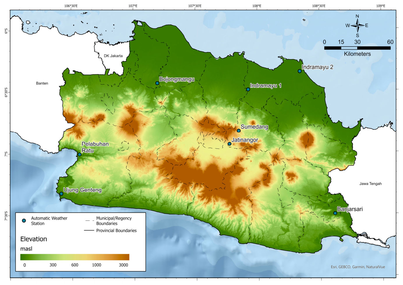
Ground-based meteorological measurements were acquired from a network of eight Automatic Weather Stations (AWS) operated by the Indonesian Agency for Meteorology, Climatology, and Geophysics (BMKG). These operational stations are geographically distributed across West Java Province to capture diverse regional microclimates. The specific locations comprising this monitoring network include Bojongmangu (BJMG), Banjarsari (BJSR), Indramayu 1 (IDMA 1), Indramayu 2 (IDMA 2), Jatinangor (JTNG), Pelabuhan Ratu (PLRT), Sumedang (SMDG), and Ujung Genteng (UJGT). Each AWS records high-frequency atmospheric data at ten-minute intervals, systematically measuring Global Horizontal Irradiance (GHI), air temperature, relative humidity, barometric pressure, wind kinematics, and precipitation. 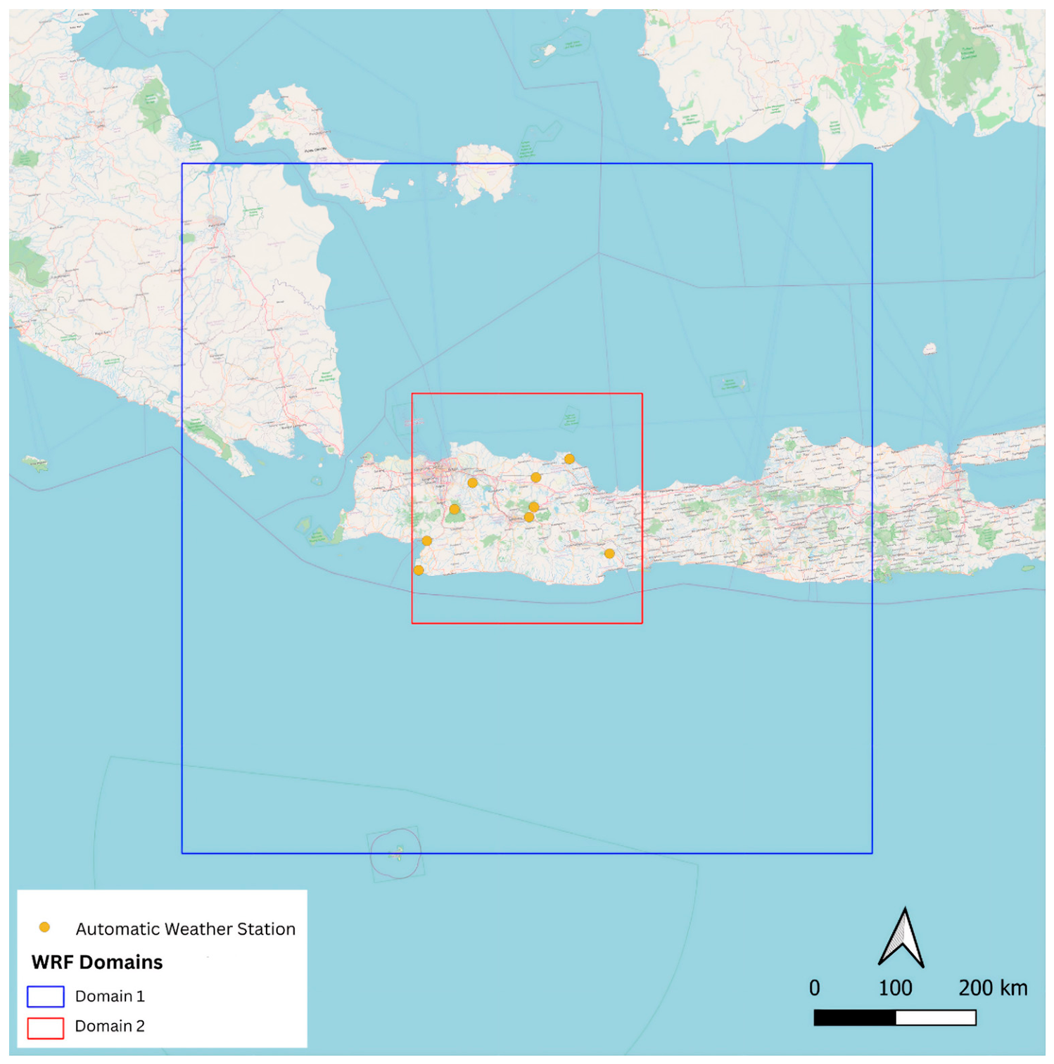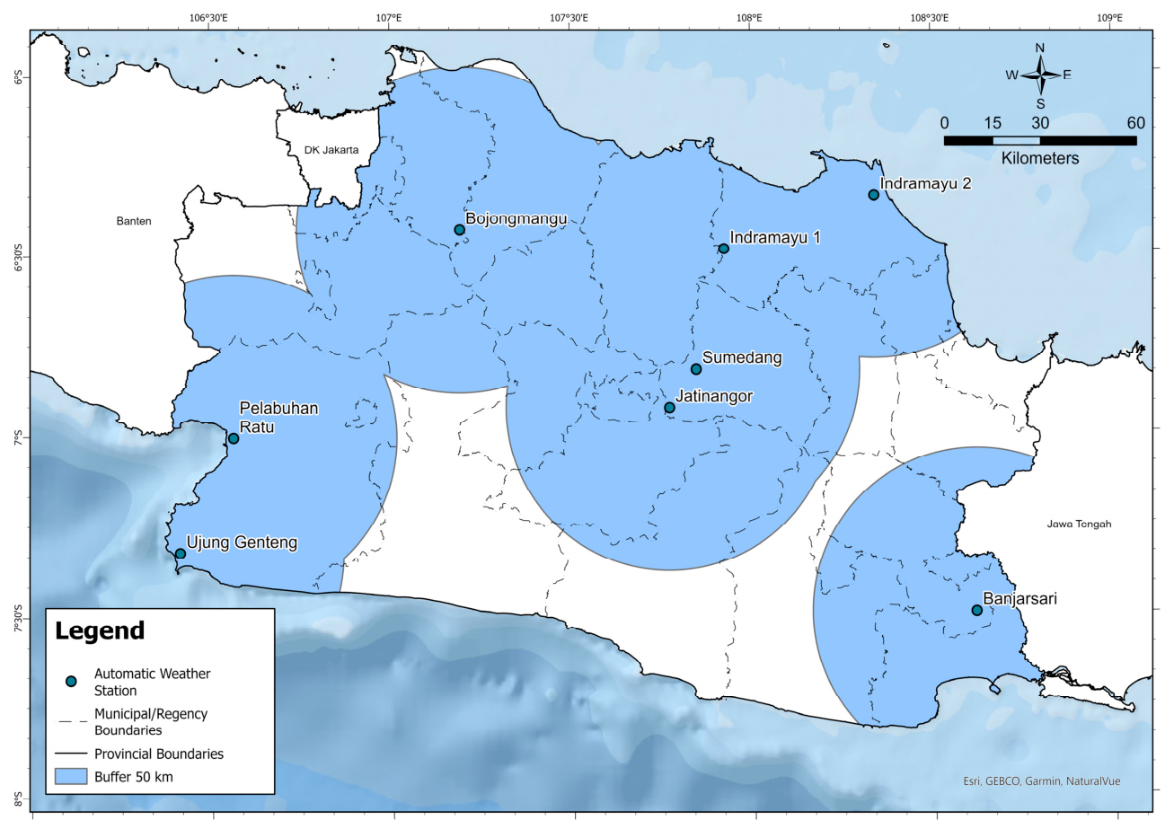Solar Zenith Angle (SZA) was computed using the pysolar Python library (version 0.13), following standard astronomical geometry formulations widely used in radiative transfer modeling [38]. The spatial distribution of AWS is presented in Figure 5.

2.1.2. Satellite Data

Visible band reflectance and atmospheric cloud properties were obtained from the GK2A geostationary satellite operated by the Korea Meteorological Administration (KMA). These continuous satellite observations provide a native spatial resolution of 500 m and a temporal resolution of ten minutes, which were subsequently aggregated to hourly intervals to synchronize with the temporal scale of the numerical models. The specific meteorological variables extracted from this dataset include visible reflectance, cloud index, and derived cloud optical indicators. These parameters are integrated into the predictive LSTM networks because satellite cloud information dynamically quantifies cloud optical thickness and spatial cloud-field evolution, both of which are fundamental for accurately calculating the attenuation of surface solar irradiance. Satellite cloud information is widely used to enhance solar irradiance forecasting because it is sensitive to cloud optical thickness and cloud-field dynamics [14,39,40].

2.1.3. Static Geospatial Data

To parameterize the lower boundary conditions of the WRF simulation, static geospatial layers were retrieved utilizing the GIS4WRF plugin integrated within the QGIS environment. These geographical inputs incorporate essential physical variables, including elevation data derived from the Shuttle Radar Topography Mission (SRTM), land cover classifications, vegetation indices, surface albedo, alongside localized terrain slope and aspect calculations. The foundational datasets supporting these specific surface parameters were aggregated from institutional repositories, including NASA, NCEP, BNU, and the USGS. Integrating data from these diverse repositories ensures that the model’s computation of land-atmosphere fluxes remains consistent with methodologies utilized in terrestrial energy balance studies.

2.1.4. Global Atmospheric Forcing

To establish the synoptic-scale atmospheric conditions for the study region, meteorological fields were extracted from the National Centers for Environmental Prediction (NCEP) Global Forecast System (GFS) ds084.1 archive. This specific dataset provides a three-hourly temporal resolution and a 0.25-degree spatial resolution, uniformly initialized at 00 UTC for each simulation cycle. These global datasets supply critical atmospheric variables, such as vertical temperature profiles, relative humidity, wind vectors, and sea-level pressure, which are fundamentally required to force the WRF model. Consequently, GFS data is widely utilized as the standard for establishing both the initial and dynamic lateral boundary conditions within the WRF framework to conduct rigorous solar irradiance simulations [16,24,25].

2.1.5. Harmonization for LSTM Input

To resolve observational gaps within the AWS time series, missing values were corrected using linear interpolation [41]. Subsequently, all predictive features were normalized via Min–Max scaling prior to model ingestion to ensure balanced gradient convergence during LSTM training. A comprehensive summary of these specific datasets and their corresponding parameters is provided in

Table 2. Summary of data sources and parameters used in this study.

Source	Parameter	Acquisition Date
BMKG	Global Horizontal Irradiance (GHI)	1 January–31 December 2023
	Air Temperature (°C)
	Wind Direction (°)
	Wind Speed (m/s)
	Air Pressure (hPa)
	Relative Humidity (%)
	Precipitation (mm)
	Solar Zenith Angle (SZA)	Computed from station coordinates
KMA (GK2A Satellite)	Visible band reflectance values	1 January–31 December 2023

.

2.2. WRF Model and Preprocessing

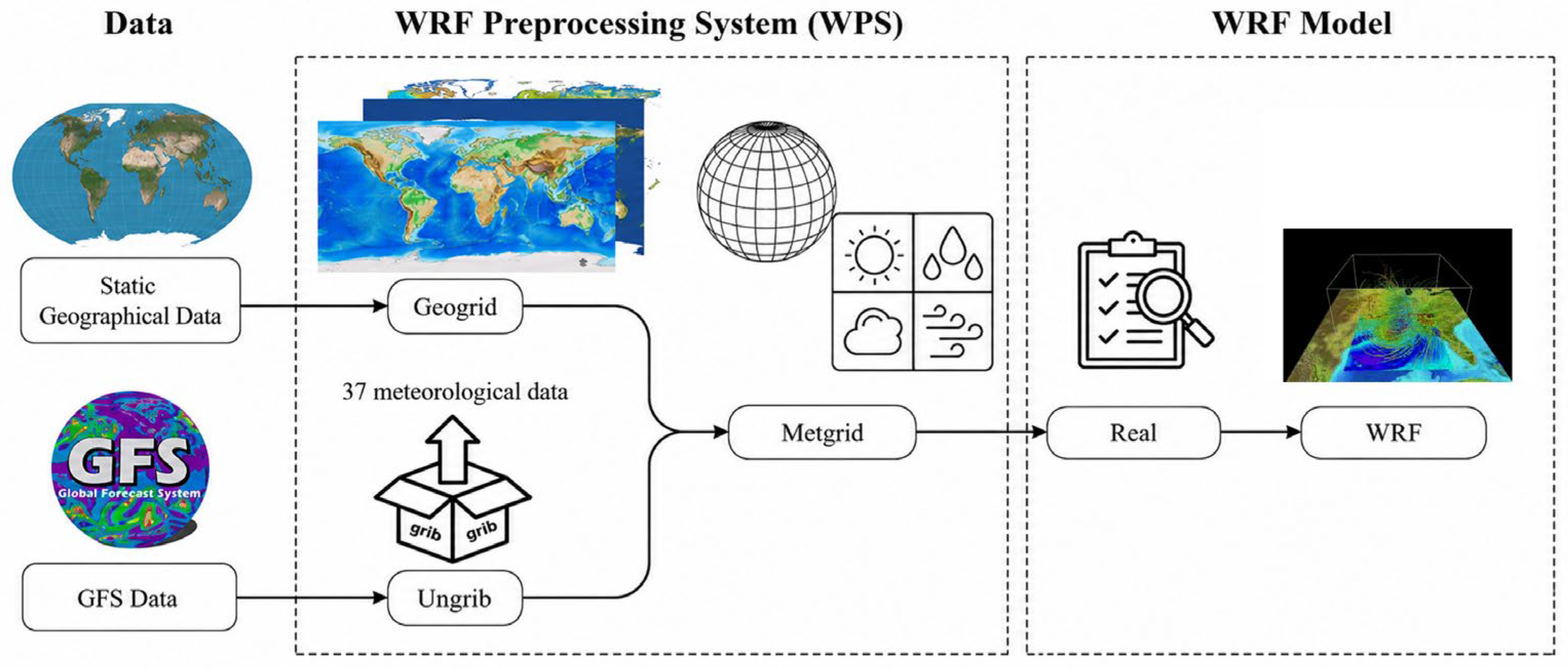
The WRF Preprocessing System (WPS) was used to ingest static geographic data, GFS boundary conditions, and surface variables through three modules. These modules, geogrid, ungrib, and metgrid, each performed distinct preprocessing functions within the workflow. The complete outline of the WPS and WRF model workflow, from static geographical and GFS data ingestion to model-ready inputs for WRF, is illustrated in Figure 6.

The geogrid module established the spatial framework of the simulation domain by calculating specific latitude and longitude coordinates derived from the namelist.wps configuration file. Within this defined boundary, the module interpolated static geographical parameters, such as terrain elevation, soil type, and the USGS 24-category land use dataset, to ensure accurate terrestrial representation across the computational grid. Concurrently, the ungrib module processed GRIB-formatted meteorological fields from the NCEP GFS ds084.1 archive, extracting 37 atmospheric variables across multiple temporal and vertical levels. These extracted variables, which include fundamental drivers such as temperature, pressure, humidity, and wind, were subsequently reformatted into intermediate files specifically compatible with the broader WPS architecture. Finally, the metgrid module integrated these data streams by applying horizontal and vertical interpolation techniques to align the extracted GFS meteorological variables with the precise spatial and pressure configurations of the geogrid-defined domain. Ultimately, this sequential three-module preprocessing pipeline ensured the seamless integration of static geographical inputs with dynamic meteorological boundary conditions prior to WRF model execution.

The WRF domain setup used nested domains with a horizontal grid spacing of 30 km (Domain 1) and 10 km (Domain 2). This provided sufficient resolution to capture mesoscale features that influence irradiance, such as coastal breezes, convective buildup, and mountain–valley circulations [21]. The overall WRF model configuration, including domain nesting and grid resolution, is summarized in Figure 7.

The WRF model was utilized to predict solar irradiance using the GIS4WRF plugin integrated within QGIS version 3.34.11 ‘Prizren’. The simulation used a hierarchical grid configuration with a child-to-parent ratio of 3:1, providing higher resolution for localized meteorological phenomena while maintaining computational efficiency. The simulation employed two domains: Domain 1 (parent domain) and Domain 2 (child domain), with Domain 2 providing finer grid spacing to model meteorological dynamics across West Java with greater precision. Both domains were designed with a 31 × 31-pixel grid. Grid spacing was set to 30 km for Domain 1 and 10 km for Domain 2, balancing computational efficiency with the ability to capture finer-scale atmospheric details. The simulation’s center was located at the BMKG’s AWS in Sumedang (latitude: −6.82349, longitude: 107.81658). This strategic placement ensured comprehensive regional coverage, including the northernmost station at Indramayu 2 (−6.34439, 108.34113), the easternmost station at Banjarsari (−7.49796, 108.61577), and the southwesternmost station at Ujung Genteng (−7.32476, 106.41298).

To achieve a high-resolution vertical profile, the model employed 33 vertical layers, facilitating detailed analysis of atmospheric processes across altitudes. The Thompson microphysics scheme was chosen for its robust performance in simulating convective precipitation, particularly under tropical conditions [42]. Radiative transfer processes, both longwave and shortwave, were parameterized using the RRTMG scheme, known for its precise representation of cloud-aerosol interactions and computational efficiency [43].

Surface-layer dynamics were modeled using the MM5 surface layer scheme, ensuring reliable simulations of momentum and heat exchange under varying atmospheric stability conditions [44]. Land-atmosphere interactions were captured using the Noah Land Surface Model, which provides high fidelity in simulating soil moisture and surface fluxes [45]. The MYNN planetary boundary layer scheme was employed to capture turbulent mixing processes, essential for accurate boundary layer dynamics [46]. Convective processes were parameterized using the Kain-Fritsch scheme, known for its effectiveness in representing updrafts and precipitation development [47]. Additionally, urban heat island effects were incorporated through the Single-layer Urban Canopy Model, enhancing the simulation of energy fluxes within urban environments [48]. WRF provides hourly forecasts of downward shortwave radiation, cloud cover, water vapor, wind components, and other atmospheric profiles relevant for irradiance forecasting. A full overview of the WRF model configuration is provided in

Table 3. Configuration of the WRF model applied in this study.

Configuration	Details
Horizontal grid spacing (for child domain)	10 km
Child-to-parent ratio	3
Center point	Longitude: 107.81658
	Latitude: −6.82349
Grid size	Horizontal: 31
	Vertical: 31
Padding	Top: 10
	Left: 10
	Right: 10
	Bottom: 10
Vertical layers	33
Microphysics	Thompson
Longwave radiation	Rapid Radiative Transfer Model for GCMs (RRTMG)
Shortwave radiation	Rapid Radiative Transfer Model for GCMs (RRTMG)
Surface layer	MM5
Land surface	Noah Land Surface Model
Planetary boundary layer	Mellor-Yamada Nakanishi and Niino with Turbulent Kinetic Energy advection
Cumulus Parameterization	Kain-Fritsch Scheme
Urban physics	Single-layer Urban Canopy Model

.

Following the execution of the WRF simulation, the gridded outputs required spatial refinement exclusively for visualization purposes. The native 10 km grid resolution of the child domain produces pixelated spatial fields that can visually mask subtle meteorological transitions. To mitigate this visual artifact, spatial maps during daylight hours were refined using cubic convolution interpolation; this generated seamless radiation fields and minimized the pixelation that might otherwise hide fine spatial gradients [49]. Crucially, this smoothing technique was applied uniformly across all mapped results—meaning both the baseline WRF outputs and the corrected spatial fields from all site-adaptation schemes were interpolated to ensure visual consistency. However, this interpolation was applied solely for graphical representation; all quantitative and statistical analyses utilized the original 10 km grid data to preserve the numerical integrity of the simulation.

2.3. SZA and AWS Data Processing

SZA was calculated using the Python pysolar library, which allowed for the accurate determination of both SZA and solar azimuth. These calculations were based on the observation date, UTC, the geographic coordinates of each station, and the satellite’s location at the time of data collection. Through the use of the get_altitude and get_azimuth functions, which return the Sun’s elevation and azimuth angles (measured in degrees clockwise from true north), the corresponding SZA and solar azimuth values were derived [50].

The raw data obtained from AWS includes variables such as rainfall, humidity, temperature, air pressure, wind speed, and wind direction. These datasets often contain missing values at certain time intervals, necessitating preprocessing to ensure data completeness and usability. To address this, linear interpolation was applied using MATLAB (R2024b). Linear interpolation estimates missing values by constructing a straight line between two known data points, ensuring smooth continuity within the dataset [41]. Additionally, the raw data, initially recorded at 10 min intervals, were aggregated to hourly intervals to create a consistent temporal framework for analysis and modeling.

2.4. LSTM Calculation and Post-Processing Model

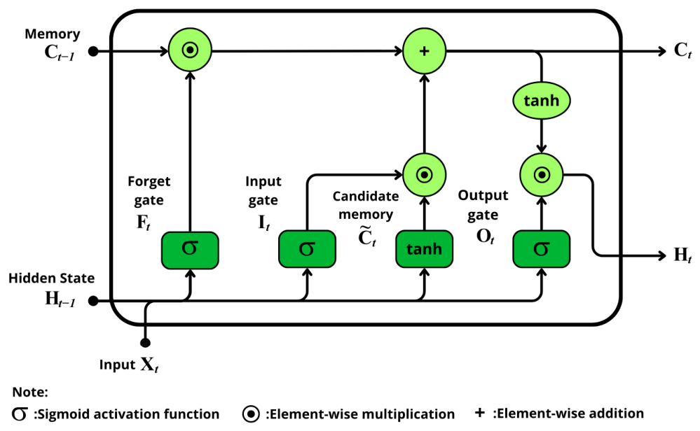
LSTM networks are a specialized form of Recurrent Neural Networks designed to handle long-term dependencies by incorporating a unique structure, including a cell state and multiple gates. These gates—forget gate, input gate, and output gate—regulate the flow of information, enabling the network to retain or discard data as needed [51]. This capability allows LSTMs to effectively model sequential data with temporal dependencies. Figure 8 illustrates the LSTM network’s architecture, showing its gated structure and core components.

Given input ${\mathrm{x}}_{\mathrm{t}}$, the previous hidden state ${\mathrm{h}}_{\mathrm{t}-1}$, and the previous cell state ${\mathrm{C}}_{\mathrm{t}-1}$, the LSTM processes information in four main steps:

The forget gate determines which information from ${\mathrm{C}}_{\mathrm{t}-1}$ to discard. It uses a sigmoid activation function, outputting values between 0 (completely forget) and 1 (fully retain):

$${\mathrm{f}}_{\mathrm{t}}=\mathsf{\sigma }\left({\mathrm{W}}_{\mathrm{f}}\cdot \left[{\mathrm{h}}_{\mathrm{t}-1},{\mathrm{x}}_{\mathrm{t}}\right]+{\mathrm{b}}_{\mathrm{f}}\right)$$

(1)

Here, ${\mathrm{f}}_{\mathrm{t}}$ is the forget gate’s output, ${\mathrm{W}}_{\mathrm{f}}$ and ${\mathrm{b}}_{\mathrm{f}}$ are its weights and biases, and σ is the sigmoid activation function [52].

Input Gate and Candidate Cell State: the input gate identifies which new information to incorporate into the cell state, while the candidate cell state generates potential updates using a hyperbolic tangent (tanh) activation:

$${\mathrm{i}}_{\mathrm{t}}=\mathsf{\sigma }\left({\mathrm{W}}_{\mathrm{i}}\cdot \left[{\mathrm{h}}_{\mathrm{t}-1},{\mathrm{x}}_{\mathrm{t}}\right]+{\mathrm{b}}_{\mathrm{i}}\right)$$

(2)

$$\widetilde{{\mathrm{C}}_{\mathrm{t}}}=\tanh \left({\mathrm{W}}_{\mathrm{C}}\cdot \left[{\mathrm{h}}_{\mathrm{t}-1},{\mathrm{x}}_{\mathrm{t}}\right]+{\mathrm{b}}_{\mathrm{C}}\right)$$

(3)

Here, ${\mathrm{i}}_{\mathrm{t}}$ represents the input gate’s output, $\widetilde{{\mathrm{C}}_{\mathrm{t}}}$ is the candidate cell state, and ${\mathrm{W}}_{\mathrm{i}}$, ${\mathrm{W}}_{\mathrm{C}}$ and ${\mathrm{b}}_{\mathrm{i}}$, ${\mathrm{b}}_{\mathrm{C}}$ are their respective weights and biases [53].

Cell State Update: the cell state is updated by combining information from the forget gate and the input gate:

$${\mathrm{C}}_{\mathrm{t}}={\mathrm{f}}_{\mathrm{t}}\cdot {\mathrm{C}}_{\mathrm{t}-1}+{\mathrm{i}}_{\mathrm{t}}\cdot \widetilde{{\mathrm{C}}_{\mathrm{t}}}$$

(4)

This equation integrates retained information from ${\mathrm{C}}_{\mathrm{t}-1}$ and new information from $\widetilde{{\mathrm{C}}_{\mathrm{t}}}$, ensuring the cell state reflects both past and present relevance [52].

Output Gate and Final Output: The output gate determines which information from the updated cell state ${\mathrm{C}}_{\mathrm{t}}$ contributes to the current output. A sigmoid function regulates the gate, and a tanh function activates the cell state:

$${\mathrm{o}}_{\mathrm{t}}=\mathsf{\sigma }\left({\mathrm{W}}_{\mathrm{o}}\cdot \left[{\mathrm{h}}_{\mathrm{t}-1},{\mathrm{x}}_{\mathrm{t}}\right]+{\mathrm{b}}_{\mathrm{o}}\right)$$

(5)

$${\mathrm{h}}_{\mathrm{t}}={\mathrm{o}}_{\mathrm{t}}\cdot \tanh \left({\mathrm{C}}_{\mathrm{t}}\right)$$

(6)

Here, ${\mathrm{h}}_{\mathrm{t}}$ represents the final output at time $\mathrm{t}$, combining relevant cell state information with output gate decisions [51].

In practice, to prevent look-ahead bias and maintain forecasting integrity, the input vector consists of BMKG AWS meteorological observations (temperature, relative humidity, wind speed, and pressure) utilized strictly as lagged historical inputs via preceding sliding windows, coupled with future WRF physical forecasts. Within this framework, the forget gate discards outdated weather influences from the previous cell state. Concurrently, the input gate and candidate state determine which fresh patterns from these lagged observations and future physical trajectories should update the memory. This combined update retains both past local trends and dynamic synoptic signals in proportion to their relevance. Finally, the output gate filters this enriched internal state to produce the hidden state, which is linearly mapped to predict the localized GHI physical residual at the target time.

LSTM networks effectively capture long-term dependencies in meteorological time series and rectify systematic residual errors in NWP irradiance forecasts [17,18,31,54,55,56]. They enhance temporal precision in areas where WRF falters on tropical convective variability. The architectural framework of the LSTM network includes stacked LSTM layers, each with 12–48 units, along with dropout and recurrent dropout, a fully connected output layer, and the Adam optimizer with early stopping.

Following multimodal deep learning guidelines, input features comprise WRF simulations and GK2A satellite data (cloud index, reflectance) [57,58]. After filling minor BMKG AWS gaps via linear interpolation, the dataset was partitioned chronologically into a 70% training set (1 January–15 September 2023) and a 30% independent test set (16 September–31 December 2023). To strictly prevent look-ahead bias, Min–Max normalization parameters were derived exclusively from the training partition and applied passively to the test set. This chronological splitting eliminates temporal overlap across the sliding windows (24, 48, 72 h), using MAE and RMSE as training loss metrics [59]. The systematic mapping of these variables, highlighting their temporal sources, physical types, and real-time operational availability across the forecast horizons, is detailed in

Table 4. Temporal source mapping and operational availability of LSTM input features across forecast horizons.

Input Variable	Data Source	Feature Type	Temporal Reference for Target Forecast Hour (t)	Operational Availability at Forecast Initialization (T_init)
Downward Shortwave Flux (GHI)	WRF Model	Forecast Quantity	Target forecasting hour (Future)	Fully Available (Simulated in advance by WRF)
GHI (Historical)	BMKG AWS	Observation	24, 48, or 72 h prior to forecast launch	Fully available (Historically recorded prior to forecast start)
Temperature, Relative Humidity, Wind Speed, Air Pressure	BMKG AWS	Observation	24, 48, or 72 h prior to forecast launch	Fully available (Historically recorded prior to forecast start)
Cloud Index	GK2A Satellite	Observation	24, 48, or 72 h prior to forecast launch	Fully available (Historically recorded prior to forecast start)
Visible Reflectance	GK2A Satellite	Observation	24, 48, or 72 h prior to forecast launch	Fully available (Historically recorded prior to forecast start)

.

Adjusting the hyperparameters of the LSTM model is essential for optimizing the performance of the LSTM model.

Table 5. Hyperparameter Search Range.

Hyperparameter	Range
Learning rate	0.0001, 0.001, 0.015, 0.01, 0.1
Optimization solver	Adam, SGD, and RMSprop
Feature scaling	Min-max, standard scaler
Number of layers	1, 3, 5, 7
Hidden nodes	12, 24, 48, 96, 128, 192
Batch size	1, 20, 24, 48, 86
Number of epochs	100, 150, 250, 500, 1000

illustrates that the learning rate, which controls weight updates, was tested in the range of 0.0001 to 0.1. A high learning rate risks overshooting the optimal solution, while a low rate slows convergence [60]. The optimizer is another key parameter, with Adam, SGD, and RMSprop being evaluated. Adam was favored for its adaptive learning rate and fast convergence.

Feature scaling, using min-max or standard scaling, ensured balanced gradients and faster convergence. The number of layers (1–7) and hidden nodes (12–192) were tuned to balance model complexity and the risk of overfitting [61]. Additionally, batch size (1–86) influenced training efficiency, with smaller sizes improving adaptability and larger ones enhancing speed [59]. The number of epochs (100–1000) was adjusted to avoid underfitting or overfitting. Optimal hyperparameters were identified through iterative testing to suit the dataset’s characteristics, achieving a balance between accuracy and efficiency.

2.5. Hybrid WRF–LSTM Forecasting Framework

The proposed hybrid architecture functions in two sequential stages. Initially, the WRF model generates the baseline physical forecasts of GHI derived from synoptic atmospheric parameters. Subsequently, the LSTM network is trained to learn the non-linear residuals between these WRF-predicted GHI values and the empirical AWS observations. Within this framework, the LSTM operates as an adaptive post-processing mechanism, explicitly refining the physical WRF outputs to resolve sub-grid cloud dynamics and align with ground truth. This approach leverages the spatial continuity of numerical modeling alongside the temporal precision of deep learning. Mathematically, the hybrid system corrects the WRF biases using the LSTM-estimated residuals according to the following equation:

GHI_Hybrid = GHI_WRF + f_LSTM(Residual)

(7)

2.6. Spatial Site Adaptation Procedure

Site adaptation refers to the process of using a short period of high-quality ground measurements at a given location to correct or adjust a longer-term modeled or satellite-derived solar irradiance dataset. This adjustment ensures that the resulting time series better represents the local (site-specific) radiation conditions. The core idea is to reduce bias, correct distributional mismatches, and improve the reliability of irradiance inputs for downstream applications (e.g., energy yield estimation, forecasting, and mapping) [33,34].

In many solar-resource studies, site adaptation is applied at individual points where ground measurements exist. Common techniques include linear regression (to reduce bias) followed by empirical quantile mapping to align statistical distributions (e.g., percentiles) between modeled and observed data [34]. Other authors have extended or modified that approach. For example, by exploring different distribution-mapping techniques (e.g., quantile delta mapping, polynomial ECDF fitting) or by hybrid sequential corrections (first regression, then distribution mapping) [36]. Machine-learning-based site adaptation methods have also been proposed, training ML models (e.g., random forests, neural nets) to predict the correction needed based on state variables and model outputs [35].

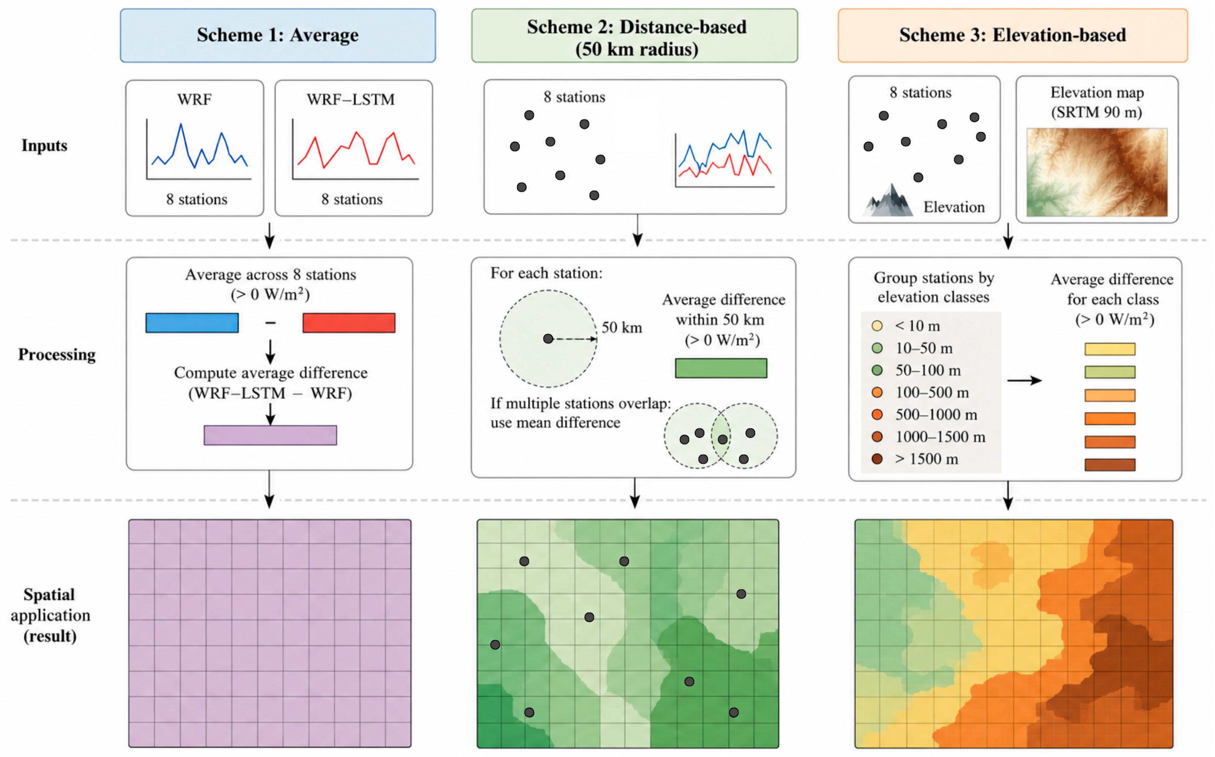
However, traditional and ML-based methods usually operate pointwise, correcting each site individually and focusing on temporal distribution alignment. In contrast, the proposed work applies geospatial transfer of corrections from stations to surrounding grid cells, forming a regional site-adaptation scheme. This approach enables full spatial coverage in data-sparse areas, captures geographic bias patterns (e.g., from elevation or terrain) that pointwise methods overlook and improves irradiance mapping for planning and grid operations. The exact workflow for integrating these three adaptation schemes is visually summarized in Figure 9 and detailed below.

2.6.1. Scheme 1: Average

In Scheme 1, the experiment averages the entire set of WRF–LSTM prediction results from eight stations during hours with solar radiation (i.e., greater than 0 W/m²). The averaged WRF values at corresponding time steps, also limited to periods with radiation greater than zero, are then subtracted from the averaged WRF–LSTM values, yielding a tabular difference. This difference is subsequently applied uniformly to all pixels within the study area. This approach is intended to provide a fair method for implementing site adaptation in areas with limited station coverage.

2.6.2. Scheme 2: Distance-Based

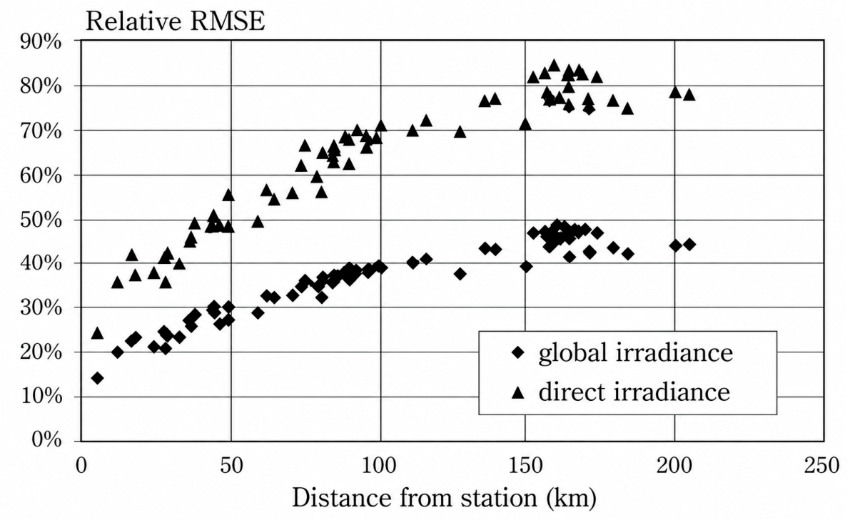
Scheme 2 adapts the 50 km threshold from [39] as a pragmatic mesoscale boundary rather than a statistical bound, given the rapid spatial decorrelation of localized tropical convection. The spatial transfer scheme is illustrated in Figure 10. This radius aligns with West Java’s atmospheric dynamics, where dominant land–sea breezes propagate roughly 60–80 km inland [62]. Restricting the spatial transfer to 50 km prevents corrections from extrapolating into distant, unmonitored territories. Where 50 km buffers intersect across the western and central domains, their WRF–LSTM differences are aggregated into a single averaged value. This approach treats the intersecting zones as a unified regional cluster, providing a smoothed, generalized correction that dampens extreme local anomalies. Conversely, geographically isolated stations apply distinct local corrections. Grid cells outside any buffer retain uncorrected WRF forecasts to ensure spatial continuity, with the scheme applied strictly during daylight hours.

2.6.3. Scheme 3: Elevation-Based

This scheme is based on the elevation of weather stations. First, the elevation of each station is identified and classified into elevation classes with designated intervals. These classes are adapted from [63], consisting of the following ranges: <10, 10–50, 50–100, 100–500, 500–1000, 1000–1500, and >1500 m. Stations falling within the same elevation class are grouped, and the average difference between the WRF and WRF–LSTM predictions is calculated for each group. This average difference is then applied to all pixels within the corresponding elevation class across the study area. Elevation data are obtained from the Shuttle Radar Topography Mission (SRTM) Digital Elevation Data Version 4, which has a spatial resolution of 90 m. As in the previous schemes, averaging is performed only during periods when solar radiation exceeds 0 W/m².

2.7. Comparison with Existing Irradiance Data

To ensure the validity of these site-adaptation results across various schemes and to identify the most effective approach, a comparison was conducted with another widely recognized solar radiation forecasting model. For this purpose, the ERA5-Land dataset was used as a reference for hourly solar radiation estimates at approximately 11.1 km spatial resolution. To align it with the WRF model’s spatial resolution (10 km), resampling techniques were applied. All schemes were conducted using the 1-day-ahead (1DA) forecast horizon, as ERA5-Land is also based on estimates [64]. Therefore, the 1DA horizon was chosen as the reference point for site adaptation due to its shortest forecast interval.

The ERA5-Land data were processed similarly to the WRF outputs. Hourly values were averaged between 08:00 and 17:00 local time (LT), corresponding to periods with solar radiation greater than 0 W/m². Subsequently, statistical metrics, including RMSE, rRMSE, MBE, rMBE, and R², were calculated to evaluate and compare the performance of WRF and WRF–LSTM across each site adaptation scheme. This operational window aligns with the active solar generation hours, complementing the astronomical SZA < 80° quality control filter applied to the raw observational data during the initial station-level pre-processing stage.

While ERA5-Land is a model-derived product rather than absolute ground truth, atmospheric reanalysis provides continuous coverage without missing values, serving as a valid alternative in data-sparse regions [65]. Consequently, ERA5-Land is utilized here strictly as an independent macro-spatial reference to evaluate relative geographical coherence, not for point-wise error validation.

2.8. Performance Evaluation Metrics

Evaluating the predictive performance of solar irradiance models necessitates robust metrics, including Root Mean Square Error (RMSE), Relative RMSE (rRMSE), Mean Bias Error (MBE), Relative MBE (rMBE), and Coefficient of Determination (R²). RMSE quantifies the average deviation between observed and predicted values, expressed in W/m², and is computed as the square root of the mean squared error. Lower RMSE values indicate superior model performance. Complementing this, rRMSE represents RMSE as a percentage of the mean observed solar irradiance, offering a normalized perspective [58].

MBE evaluates the systematic bias of predictions by determining whether the model consistently overpredicts or underpredicts, with positive values indicating overprediction and negative values suggesting underprediction. Its normalized counterpart, rMBE, expresses this bias relative to the mean observed value [58]. R², or the coefficient of determination, measures the proportion of variance in the observed data that the model explains. Values nearing 1 signify high explanatory power, while lower values suggest inadequate model performance [30]. Given SRi is the observed solar irradiance for observation i, $\widehat{\mathrm{S}{\mathrm{R}}_{\mathrm{i}}}$ is the predicted value, $\overline{\mathrm{S}\mathrm{R}}$ is the mean observed solar irradiance, and n is the total number of observations; performance metrics (RMSE, rRMSE, MBE, rMBE, and R²) formulas are computed as following Equations (8)–(12):

$$\mathrm{R}\mathrm{M}\mathrm{S}\mathrm{E}=\sqrt{{\displaystyle \frac{1}{\mathrm{n}}}{\displaystyle \sum _{\mathrm{i}=1}^{\mathrm{n}}}{\left(\mathrm{S}{\mathrm{R}}_{\mathrm{i}}-{\widehat{\mathrm{S}\mathrm{R}}}_{\mathrm{i}}\right)}^2}$$

(8)

$$\mathrm{rRMSE}={\displaystyle \frac{{\mathrm{RMSE}}_{\mathrm{S}\mathrm{R}}}{\overline{\mathrm{S}\mathrm{R}}}}\times 100$$

(9)

$$\mathrm{MBE}={\displaystyle \frac{1}{\mathrm{n}}}\sum _{\mathrm{i}=1}^{\mathrm{n}}\left(\widehat{\mathrm{S}{\mathrm{R}}_{\mathrm{i}}}-\mathrm{S}{\mathrm{R}}_{\mathrm{i}}\right)$$

(10)

$$\mathrm{rMBE}={\displaystyle \frac{\mathrm{MBE}}{\overline{\mathrm{S}\mathrm{R}}}}\times 100$$

(11)

$${\mathrm{R}}^2=1-{\displaystyle \frac{\sum {\left(\mathrm{S}{\mathrm{R}}_{\mathrm{i}}-\widehat{\mathrm{S}{\mathrm{R}}_{\mathrm{i}}}\right)}^2}{\sum {\left(\mathrm{S}{\mathrm{R}}_{\mathrm{i}}-\overline{\mathrm{S}\mathrm{R}}\right)}^2}}$$

(12)

3. Results

3.1. Data Completeness and Quality Control

Assessment of the eight AWS datasets indicates substantial variability in observational continuity, with missing fractions ranging from 0.09 to 11.06%. Persistent gaps occur during February, May, October, and late December. The QC procedures, as described in

Table 6. AWS and WRF data QC procedures and criteria [66].

Procedure/Parameters	Criteria
Interpolation	Linear from 10 min to 60 min
SZA	<80°
GHI AWS and WRF	>0 W/m2

, adapted from [66], ensured cross-station homogeneity and the derivation of hourly daytime irradiance records.

3.2. LSTM Hyperparameters

Hyperparameter optimization constitutes a critical step in training LSTM models, ensuring that each network is able to capture temporal patterns in solar irradiance data without succumbing to overfitting. Rather than relying on a one-size-fits-all configuration, multiple combinations of layer sizes, regularization rates, and training schedules were systematically evaluated to identify the most effective settings for each AWS dataset. The hyperparameter details for each AWS are listed in

Table 7. Hyperparameters applied for WRF data in each AWS.

AWS	Units	Number of Layers	Dropout Rate	Epochs	Batch Size	Optimizer	Learning Rate
BJMG	24	3	0.0001	100	20	Adam	0.001
BJSR	24	3	0.0001	100	20	Adam	0.001
IDMA 1	12	3	0.001	100	20	Adam	0.001
IDMA 2	48	3	0.0001	100	20	Adam	0.001
JTNG	24	3	0.0001	100	24	Adam	0.001
PLRT	48	3	0.0001	100	20	Adam	0.001
SMDG	24	3	0.0001	100	20	Adam	0.001
UJGT	24	3	0.0001	100	20	Adam	0.001

.

The resulting architecture employs 24 hidden units per layer for most stations, though this was adjusted to 12 for IDMA 1 and 48 for PLRT. The models utilized a baseline dropout rate of 0.0001, which was raised to 0.001 specifically at the IDMA 1 station. All models were trained for 100 epochs using the Adam optimizer with batch sizes of 20 (24 for JTNG), yielding optimal convergence and generalization across the diverse station datasets.

3.3. WRF-Derived Spatial Distribution of GHI

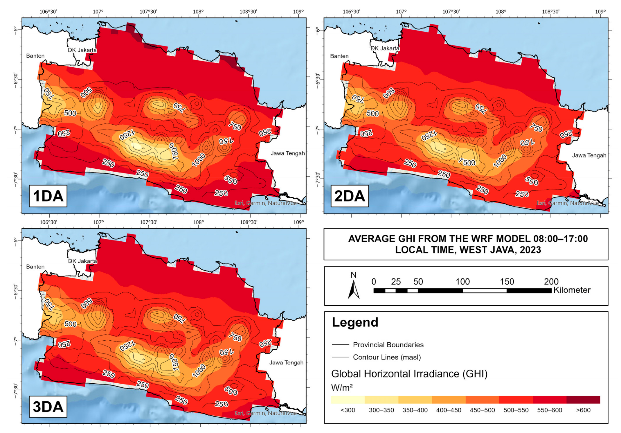
The WRF-generated spatial fields for GHI across West Java reveal a coherent climatological gradient. Computed using hourly outputs from 08:00 to 17:00 Local Time (LT), the average GHI exhibits consistent maxima reaching approximately 600 W/m² across the northern lowlands. In contrast, the central highland areas show significantly lower values, dropping to roughly 300 W/m² due to persistent orographic cloud development and complex terrain constraints. Figure 11 illustrates that this broad spatial pattern is robustly preserved across the 1DA, 2DA, and 3DA forecast horizons. However, while the topographical influence remains distinct, the spatial gradients become progressively smoother at higher lead times due to inherent model diffusion.

3.4. Performance Evaluation of the Hybrid WRF–LSTM

Table 8. Performance comparison of the WRF and WRF-LSTM models across all AWS, averaged over different forecast horizons.

Horizon	Method	RMSE (W/m2)	rRMSE (%)	MBE (W/m2)	rMBE (%)	R2
1DA	WRF	310.74	62.88	139.01	31.06	0.44
	WRF-LSTM	183.44	36.55	10.70	3.19	0.64
	Difference (∆)	127.30	26.33	128.31	27.87	0.20
2DA	WRF	300.66	63.90	157.15	35.92	0.49
	WRF-LSTM	178.80	37.17	15.30	4.11	0.67
	Difference (∆)	121.86	26.72	141.85	31.81	0.18
3DA	WRF	299.94	63.79	153.32	35.15	0.48
	WRF-LSTM	179.29	37.45	8.56	2.48	0.66
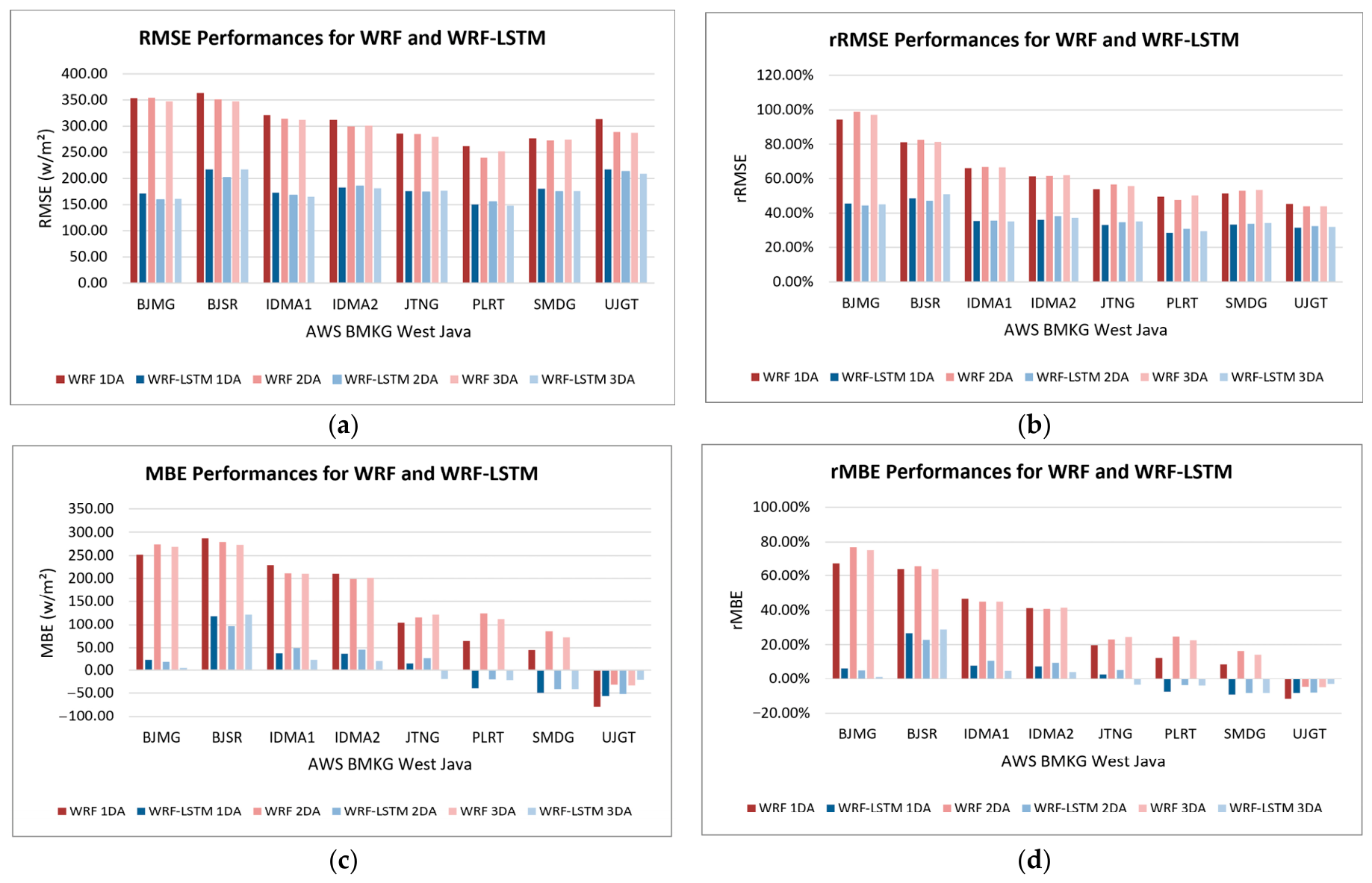
	Difference (∆)	120.66	26.34	144.76	32.66	0.18

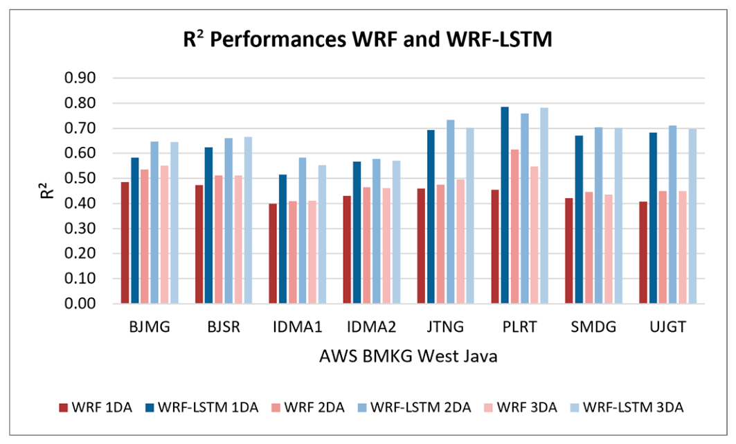
and Figure 12 illustrate the improvements achieved by the hybrid WRF–LSTM model relative to standalone WRF forecasts. Across all evaluated stations, the WRF-LSTM approach significantly reduces overall forecast errors, as demonstrated by consistent improvements in both RMSE and rRMSE. Specifically, the BJMG station exhibits the largest RMSE reduction (Δ ≈ 187.65 W/m²), whereas UJGT shows the smallest, yet still notable, improvement (Δ ≈ 83.42 W/m²). Furthermore, bias metrics such as MBE and rMBE show substantial overall enhancement, even though the UJGT station experiences a slight overcorrection in these areas.

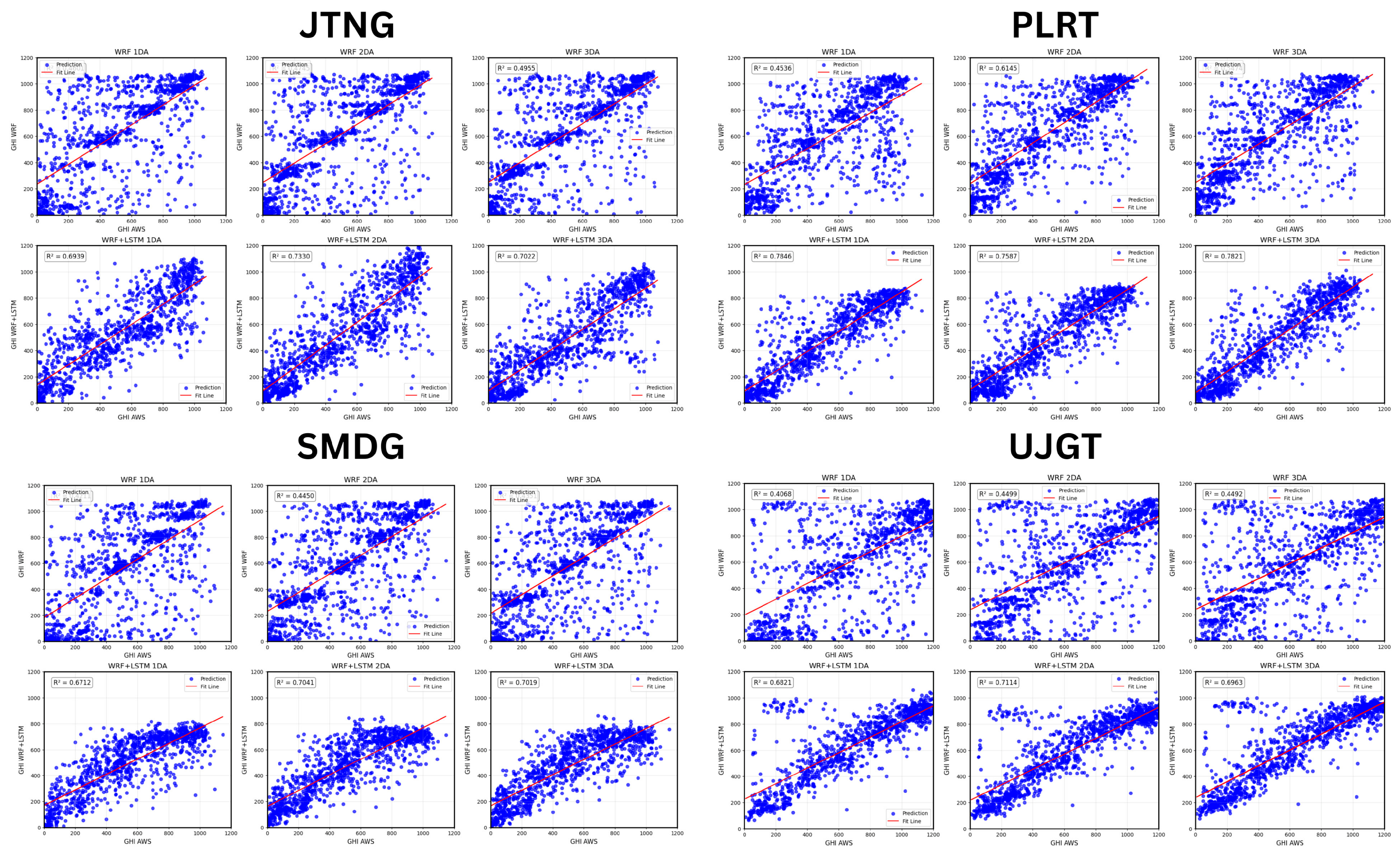
R² gains are more spatially uniform but reveal a different ranking: the largest improvements occur at stations where raw WRF skill was lowest, such as UJGT (ΔR² ≈ 0.263). In contrast, stations with high baseline skill, such as BJMG, exhibit smaller increases (ΔR² ≈ 0.10). These results indicate that the LSTM component enhances both accuracy and variance explanation, particularly at sites where the physical model struggles (Figure 13).

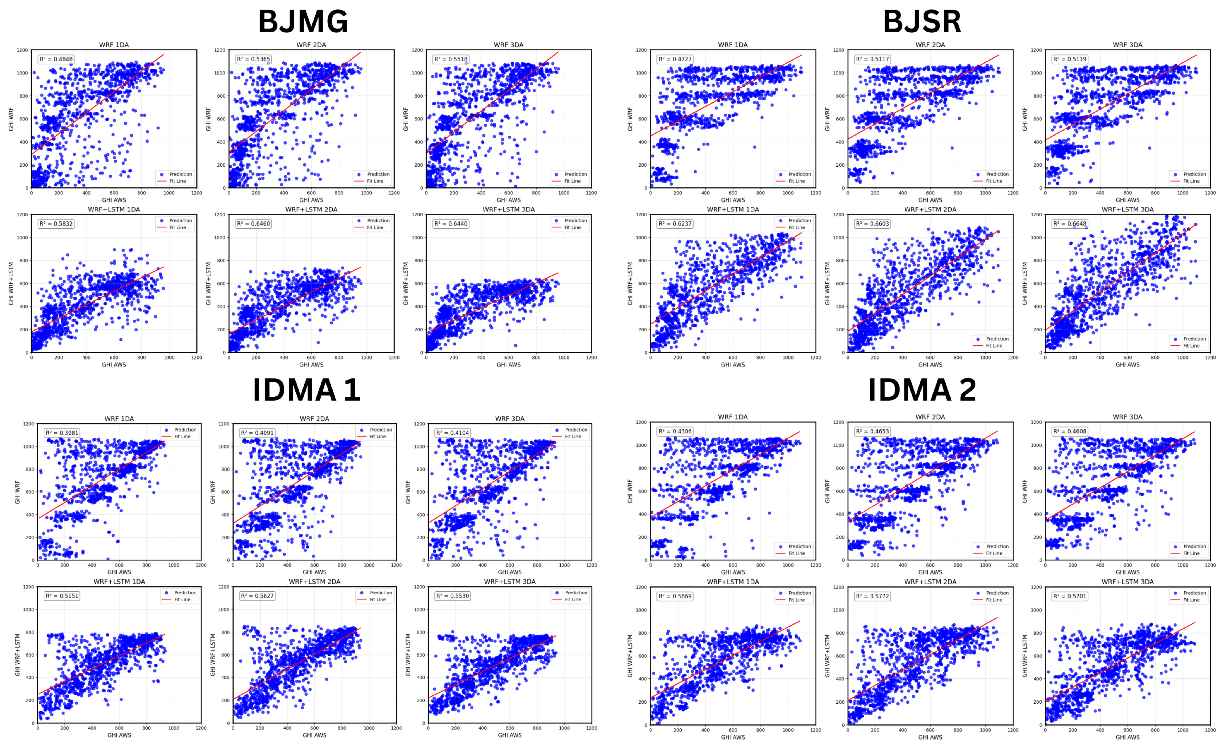
Across all AWS, the hybrid configuration demonstrably surpasses standalone WRF forecasts. RMSE decreases by ~120–127 W/m², rRMSE by more than 25%, and MBE by up to 128 W/m². R² improvements (0.18–0.20) are most pronounced at stations with low baseline WRF skill. These findings indicate that LSTM-based post-processing effectively mitigates both systematic and random errors while enhancing variance representation. In every forecast horizon, 1DA, 2DA, and 3DA, the WRF-LSTM predictions cluster more tightly around the regression line in scatter-plot visualizations, indicating a marked improvement in alignment with observed AWS measurements, as reported in Figure 14.

These performance gains confirm that the LSTM network successfully captures nonlinear dependencies. Furthermore, it corrects systematic biases arising from cloud representation errors inherent in the WRF model. This deep learning post-processing proves especially beneficial under conditions of high cloud variability, which is a hallmark of tropical convection. Additionally, while restricted to a single year (2023), the chronological 70/30 split ensures robust seasonal generalization; the 30% independent test window (16 September–31 December) successfully validates the model across the critical transition from the dry season to the highly volatile, convective onset of the wet Northwest Monsoon.

Despite these substantial improvements, certain methodological limitations persist. First, the LSTM remains intrinsically constrained by the quality of the WRF input features; poorly simulated convective initiation or dissipation by the NWP cannot be completely reversed. Second, the station-specific nature of this temporal optimization may limit direct generalization to entirely unobserved locations without further spatial adaptation. Third, the hybrid architecture inherits well-known deep learning sensitivities regarding sequence length and sampling patterns.

Nevertheless, the overall enhancement clearly demonstrates the value of combining physically informed mesoscale atmospheric structures (WRF) with data-driven temporal corrections (LSTM). This combination yields a framework that is both highly effective and computationally efficient. Ultimately, this integrated approach provides a robust solution for multi-day solar irradiance forecasting in data-sparse tropical regions.

3.5. Spatial Site Adaptation Schemes

This section evaluates the outcomes of the three spatial site adaptation schemes (Average, Distance-based, and Elevation-based) detailed in Section 2.6. The specific GHI adjustment factors applied to the regional grid are summarized in

Table 9. The differences in GHI pixel values to be subtracted from the WRF values for all three schemes.

Scheme 1		Scheme 2		Scheme 3
AWS	GHI (W/m2)	AWS	GHI (W/m2)	Elevation (masl)	GHI (W/m2)
BJMG	229.73	BJMG	229.73	0–10	172.85
BJSR	168.57	IDMA1	190.50	10–500	134.04
IDMA1	190.50	IDMA2	172.85	>500	91.88
IDMA2	172.85	JTNG	89.59
JTNG	89.59	PLRT	103.88
PLRT	103.88	SMDG	94.18
SMDG	94.18	UJGT	−22.50
UJGT	−22.50	AVG	122.60
AVG	128.35	BJSR	168.57

Note: Bold values indicate the average (AVG) GHI pixel differences for the respective schemes.

. These values represent the exact computed differentials between the baseline WRF and the optimized WRF-LSTM predictions derived from the AWS. Under the Average approach (Scheme 1), the mean differential was calculated for each station. The results indicate that BJMG exhibits the largest deviation and JTNG the smallest, while UJGT displays a distinct pattern with values consistently lower than the original predictions.

In contrast, the Distance-based approach (Scheme 2) geographically constrains the spatial application of these adjustments. Figure 15 maps the 50 km buffer radii surrounding the eight AWS in West Java. As depicted, applying corrections exclusively within these proximate zones leaves approximately 33% of the study area unadjusted, illustrating the coverage limitations inherent to station-dependent methods. Within this framework, all AWS except BJSR are located within intersecting buffer zones. Because BJSR is geographically isolated, it was treated separately and assigned a distinct correction value. For the remaining clustered stations, the WRF-LSTM differences were averaged, resulting in a mean regional correction of 122.60 W/m².

Finally, the Elevation-based approach (Scheme 3) stratifies the correction values by categorizing each AWS into specific topographical ranges. The resulting classifications include a 0–10 m above sea level (masl) range represented solely by IDMA 2, alongside a 10–500 masl range containing the majority of the stations (BJMG, BJSR, IDMA 1, PLRT, and UJGT) situated between 30 and 50 masl. Lastly, a >500 masl range comprises the high-altitude stations JTNG (753 masl) and SMDG (826 masl).

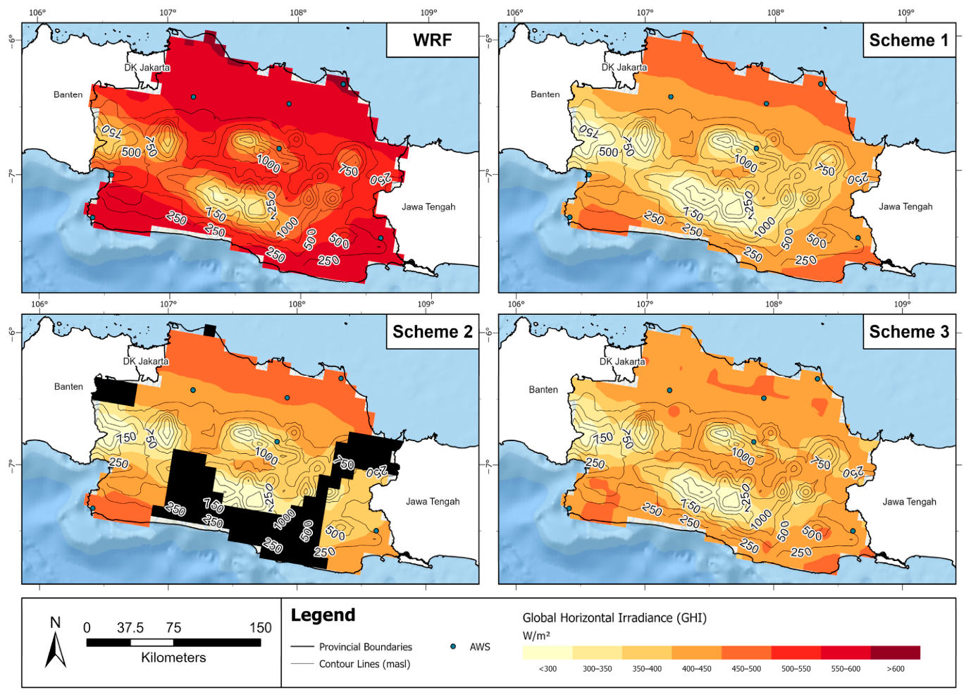
The four-panel map in Figure 16 visualizes the resulting spatial distribution of GHI across West Java under the different approaches. The raw WRF simulation displays the highest overall GHI values, particularly in the central and eastern areas where estimates frequently exceed 600 W/m². Following the application of the site-adaptation schemes, the spatial patterns alter significantly. Scheme 1 presents a uniformly moderated and spatially smoothed distribution, reducing peak GHI values and yielding a more gradual coastal-to-inland gradient. Scheme 2 displays distinct, localized adjustments confined strictly within the 50 km station buffers, resulting in visible spatial discontinuities where the uncorrected areas appear in black. Lastly, Scheme 3 yields a distribution visibly stratified by topography, reflecting distinctly lower irradiance values in higher-elevation zones, such as the southern highlands where AWS such as JTNG and SMDG are situated.

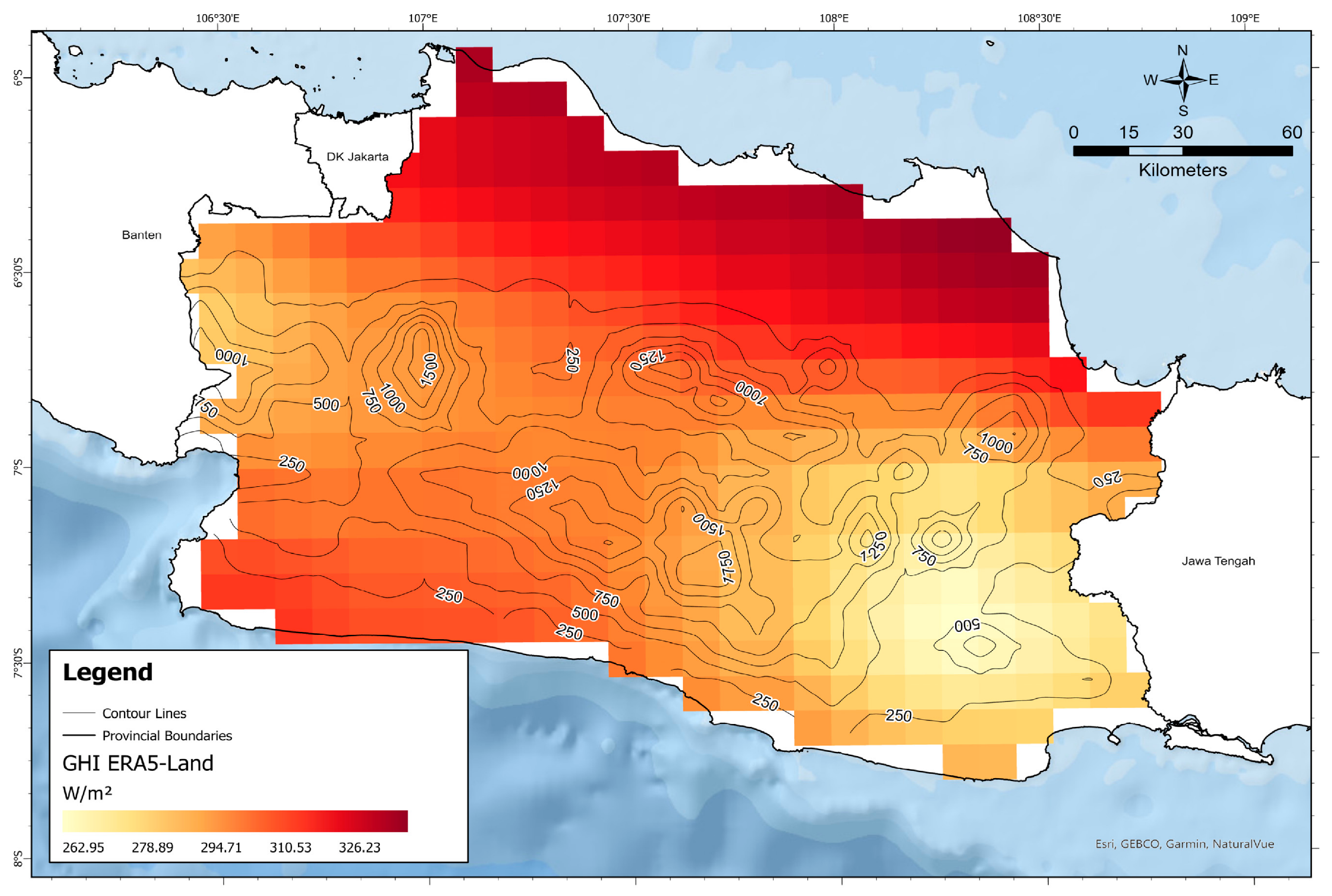
The ERA5-Land GHI map, shown in Figure 17, depicts the spatial distribution of solar irradiance across West Java at a coarse resolution of approximately 11 km. The map reveals a distinct gradient, with GHI values ranging from around 263 W/m² in the southern highlands to over 326 W/m² in the northern lowlands and coastal regions. This spatial pattern reflects the influence of topography and atmospheric conditions—lower irradiance occurs over elevated, cloud-prone areas, whereas higher values predominate in the flatter, generally drier northern zones. This map also serves as the benchmark for evaluating the accuracy of all GHI prediction schemes (WRF and WRF-LSTM with various site adaptations) using quantitative performance metrics such as RMSE, rRMSE, MBE, rMBE, and R². Since the ERA5-Land data have been processed to match the target time window of 08:00–17:00 LT and resampled accordingly, it provides a standardized, observation-constrained reference surface.

The error analysis, shown in

Table 10. Error metrics of the results of the three site adaptation schemes in comparison with GHI prediction from ERA5-Land.

	RMSE (W/m2)	rRMSE (%)	MBE (W/m2)	rMBE (%)	R2
WRF	232.61	78.72	75.31	25.48	0.17
Scheme 1	113.23	38.32	32.51	11.00	0.17
Scheme 2	114.69	38.60	25.67	8.64	0.37
Scheme 3	115.33	39.04	35.32	11.96	0.09

, reveals distinct trade-offs among the three site adaptation schemes compared to ERA5-Land. The statistical metrics presented in Table 10 were calculated on a pixel-by-pixel, hourly basis across all grid cells during the active daytime hours (08:00–17:00 LT) over the evaluation period. The raw WRF baseline exhibits large errors and a strong positive bias (rRMSE = 78.72%, rMBE = 25.48%). Scheme 1 exhibits the lowest error values (RMSE = 113.23 W/m², rRMSE = 38.32%). However, its relatively low R² (0.17) indicates that the uniform correction method does not sufficiently capture spatial variability in GHI, potentially limiting its usefulness for location-specific assessments.

Scheme 2 presents a more balanced performance. While its RMSE is only marginally higher than that of Scheme 1, it achieves the lowest mean bias error (MBE = 25.67 W/m², rMBE = 8.64%) and the highest coefficient of determination (R² = 0.37), indicating stronger spatial coherence with ERA5-Land. Specifically, these error metrics were calculated exclusively for the grid cells within the active 50 km buffers, meaning the uncovered ~33% of the West Java domain was omitted from this calculation to prevent uncorrected pixels from distorting the local transfer evaluation. This suggests that the distance-based correction, despite excluding approximately 33% of the region due to the absence of nearby stations, is more effective in addressing localized model biases where observational data are available.

Scheme 3 offers the unique advantage of continuous, full-domain topographical coverage without spatial gaps, which is conceptually essential for complex island terrains. Against regional reanalysis, it exhibits a lower spatial correlation (R² = 0.09, rRMSE = 39.04 W/m²). This outcome highlights that in highly convective tropical climates, dynamic localized cloud formations often overshadow static elevational gradients when transferring bias corrections. Additionally, because the lowest elevation band (0–10 masl) is represented by a single coastal station (IDMA 2), the transfer of corrections across different low-lying coastal microclimates is naturally constrained. Thus, Scheme 3 serves as a valuable physically guided baseline whose spatial accuracy remains closely linked to the density of the multi-elevation monitoring network.

Overall, the comparison of the three site adaptation schemes demonstrates that no single approach is universally superior across all performance metrics. Scheme 1 minimizes total error, Scheme 2 improves spatial accuracy where reference data exist, and Scheme 3 ensures continuous spatial coverage with limited precision. These findings underscore the importance of selecting a bias correction strategy that aligns with the available ground observations and the intended use of the irradiance data. As station coverage improves, especially in currently unrepresented areas, the limitation of the distance-based buffer in Scheme 2 may also diminish, allowing for more comprehensive and refined spatial corrections. It is also important to note that while ERA5-Land offers globally consistent irradiance estimates, its reanalysis-based outputs may still deviate in accuracy at regional scales due to resolution constraints and the complexity of local atmospheric conditions, further reinforcing the value of tailored, site-specific adaptation strategies.

Evaluating spatial transferability across a sparse tropical network (N = 8) presents inherent challenges for independent spatial validation, such as leave-one-station-out cross-validation. As noted by Ref. [67], spatial structures derived from small sample sizes (N < 50) are highly sensitive, as maintaining sample spacing is critical to accurately identify correlation. Consequently, omitting a station in this study would heavily disrupt the specific spatial constraints being evaluated, such as the localized buffers (Scheme 2) or the discrete terrain classes (Scheme 3). While ERA5-Land provides a useful continuous spatial benchmark, expanding the ground observation network remains an essential priority for future research to enable more robust spatial cross-validation alongside the temporally verified 30% test set.

3.6. Evaluation of Spatial Site-Adaptation Schemes

Among the three spatial adaptation methods, Scheme 2 offers a more consistent balance between spatial continuity and forecasting accuracy. Although the average-based approach (Scheme 1) yields the lowest point-level RMSE, its uniform application lacks spatial representativeness across heterogeneous landscapes. Conversely, the elevation-based approach (Scheme 3) provides continuous full-domain coverage but exhibits degraded performance, demonstrating that elevation alone is an insufficient proxy for solar irradiance gradients in the humid tropics. In equatorial regions, mesoscale atmospheric circulation and convective cloud morphology dictate surface GHI far more than static terrain effects. Consequently, Scheme 2 produces stronger spatial consistency, achieving a higher correlation (R² = 0.37) and reduced bias by integrating observational proximity with WRF’s physical forecast structures when transferring correction signals. Comparative evaluation against gridded ERA5-Land reanalysis further indicates that Scheme 2 reasonably reflects the spatial distribution and magnitude of regional GHI, highlighting its potential applicability to operational resource mapping in areas lacking dense monitoring networks. Nonetheless, while Scheme 2 exhibits more favorable spatial metrics among the evaluated methods, a static 50 km threshold remains an operational approximation that is structurally limited in capturing West Java’s highly heterogeneous microclimatic gradients. In convective tropical island environments, point-to-point GHI spatial correlation decays rapidly over short distances, rendering a uniform spatial buffer insufficient to fully resolve localized cloud-attenuation patterns.

3.7. Recommendations and Future Research Directions

Several extensions can further improve hybrid irradiance forecasting. Higher-resolution cloud microphysics—or ensemble WRF configurations—may help reduce biases during convectively active periods [42,47]. Integrating satellite-derived cloud optical properties more explicitly into the LSTM input space could enhance responsiveness to rapidly evolving cloud fields [68].

Future work should explore advanced spatio-temporal architectures, such as transformer-based models, convolutional LSTMs, and graph neural networks, to capture highly non-linear cloud dynamics. Implementing uncertainty quantification frameworks—including Bayesian deep learning and ensemble post-processing—will also be critical to enhance the operational reliability of day-ahead forecasts for PV grid integration. On the spatial front, to overcome the inherent limitations of static distance-based assumptions, future research must prioritize developing dynamic, variable buffer zones modeled as a function of localized elevation, convective cloud regimes, and microclimatic factors, as a uniform 50 km radius is structurally insufficient to represent West Java’s terrain complexity. Integrating these dynamic buffers with advanced geostatistical or machine learning-based spatial transfer techniques will yield superior regional generalization across complex landscapes. Finally, as Indonesia’s ground-based monitoring network expands, future work will prioritize executing rigorous spatial validation protocols, such as leave-one-station-out cross-validation, to verify model transferability across completely unobserved domains.

4. Conclusions

The WRF simulations reproduced the dominant north–south gradient in surface irradiance across West Java but continued to exhibit systematic overestimation and increasing uncertainty at longer lead times. By incorporating historical model–error relationships, the hybrid WRF-LSTM framework substantially enhanced forecast skill, reducing RMSE and bias while consistently increasing correlation across all stations. Performance gains were largest in areas with initially high WRF errors, and the improvements remained stable for 1- to 3-day lead times, indicating strong potential for operational solar energy planning.

To extend local corrections spatially, three site-adaptation strategies were assessed. The distance-based approach provided the best balance between accuracy and spatial continuity, while the mean- and elevation-based methods each exhibited clear trade-offs between coverage and precision. These findings highlight the importance of integrating both observational proximity and mesoscale spatial structure when transferring corrections across heterogeneous tropical terrain. Comparisons with ERA5-Land further show that global reanalysis can offer stable large-scale patterns but remains limited in representing local cloud and terrain effects.

Future work should prioritize increasing AWS network density. Additionally, exploring higher-resolution or ensemble WRF configurations will help to further refine spatial adaptation. Integrating satellite-derived cloud properties and implementing advanced machine learning architectures may offer additional gains for real-time irradiance forecasting in data-sparse tropical regions.