Article

Evaluating Landsat Water Indices and Monitoring Long-Term Surface-Water Dynamics in Lake Nasser and the Tushka Lakes in a Hyper-Arid Environment Using Google Earth Engine

1
Geology Department, Faculty of Science, Sohag University, Sohag 82524, Egypt
2
Astronomy, Space Science and Meteorology Department, Faculty of Science, Cairo University, Cairo 12613, Egypt
*
Author to whom correspondence should be addressed.
Earth 2026, 7(4), 112; https://doi.org/10.3390/earth7040112
Submission received: 14 May 2026 / Revised: 28 June 2026 / Accepted: 2 July 2026 / Published: 5 July 2026
(This article belongs to the Special Issue Feature Papers for AI and Big Data in Earth Science)

Abstract

Long-term monitoring of surface-water dynamics in hyper-arid reservoir systems requires consistent remote-sensing methods that can distinguish open water from bright desert surfaces, shallow water, wet sand, and mixed shoreline pixels. This study evaluates Landsat-derived spectral water indices for delineating surface water in Lake Nasser and the adjacent Tushka Lakes, generates a multi-decadal record of surface-water extent using Google Earth Engine, and places the resulting surface-water patterns in the context of available hydrogeological observations. Landsat TM and OLI surface reflectance imagery was used to compare seven commonly applied water indices (NDWI, EWI, NDX, WRI, AWEInsh, TCW, and NWI) based on mapped water area, relative area differences, and classification accuracy metrics derived from 1000 stratified reference samples. Among the tested indices, NDWI provided stable water–land separation (overall accuracy ≈ 93.6%; κ ≈ 0.898) and was selected for long-term mapping. The NDWI-based workflow was implemented in Google Earth Engine to generate quarterly composites of surface-water extent for the period 1987–2026. The resulting time series reveals stable, persistent surface water in the central and southern sectors of Lake Nasser, in contrast to pronounced seasonal and interannual variability in the shallow, intermittently connected Tushka basins. Total mapped water area increased from 2631 km2 in 1987 to 8923 km2 in early 2026, with Lake Nasser ranging from 2411 to 6060.7 km2 and the Tushka Lakes expanding from no mapped water before 1998 to more than 3300 km2 during 2025. To assess possible surface–subsurface interaction, daily lake-stage records (1965–2014) and monthly groundwater levels from 44 observation wells were used to estimate potential seepage losses from Lake Nasser to the Nubian Sandstone Aquifer System using Darcy’s law. Annual seepage estimates ranged from 15.58 × 10⁶ to 36.68 × 10⁶ m3/year, suggesting spatial variability in potential lake–aquifer seepage along the western lake margin. The combined remote-sensing and hydrogeologic results provide complementary, non-causal evidence for interpreting where surface-water persistence and estimated seepage may co-occur. Because spatial correlation analysis, calibrated ground-water modeling, full water-budget analysis, and independent field validation were not performed, the inferred seepage–surface-water relation should be regarded as a cautious hypothesis rather than proof of causality.

1. Introduction

Monitoring surface-water dynamics in large desert reservoirs is essential for understanding hydrologic variability, evaluating water-resource security, and supporting sustainable management under changing climatic and upstream regulatory conditions [1,2,3,4]. In Egypt, Lake Nasser and the adjacent Tushka Lakes form a strategically important and highly dynamic surface-water system in which the water extent varies over time in response to reservoir operations, hydrologic forcing, local topography, and surface–subsurface interactions [5,6,7]. Because these water bodies occupy a hyper-arid environment characterized by shallow shorelines, intermittent connectivity, and spectrally complex surrounding terrain, they provide a valuable natural setting for testing geospatial methods for water detection and long-term monitoring [8].
Recent advances in cloud-based geospatial analysis have expanded the capacity to process large Earth-observation archives by integrating remote sensing, automated preprocessing, reproducible scripting, and spatial analytics [9,10,11]. Within this context, the Landsat program offers one of the most valuable resources for long-term inland-water monitoring because it provides multi-decadal, moderate-resolution imagery suitable for consistent change analysis [12,13]. However, reliable extraction of water extent from Landsat imagery depends strongly on the performance of spectral water indices, which may vary across sensors and environmental conditions [14]. In arid reservoir settings such as Lake Nasser and the Tushka Lakes, index performance can be influenced by turbidity, shallow-water effects, mixed shoreline pixels, dark desert surfaces, and seasonal fluctuations in inundation patterns [15].
Previous studies have established a strong foundation for satellite-based monitoring of inland water bodies. Global and regional investigations have shown that multi-temporal satellite imagery can be used to map surface-water occurrence, lake-area change, and reservoir dynamics over long periods [4,9,10]. Other studies have focused on the development and comparison of spectral water indices, including NDWI, MNDWI, AWEI, WRI, TCW, and related formulations, demonstrating that index performance depends on sensor characteristics, threshold choice, water turbidity, background land cover, and shoreline conditions [11,12,13,14,15,16]. Recent cloud-computing studies have further shown that Google Earth Engine and automated workflows can efficiently process large Landsat archives for water mapping, trend detection, and near-operational monitoring [17,18,19,20]. These studies confirm the general value of Landsat and cloud-based analysis for surface-water monitoring, but they also emphasize that no single water index performs optimally in all environments and that local validation remains necessary.
For the Lake Nasser–Tushka region specifically, earlier research has addressed several related aspects of the system. Remote sensing and GIS studies monitored Lake Nasser morphology, surface area fluctuations, and environmental characteristics, while altimetry-based studies evaluated water-level variability and short-term changes in lake area [21,22]. Other studies examined the formation, expansion, contraction, and water-budget behavior of the Tushka Lakes, including the role of evaporation and groundwater recharge in lake-volume loss [5,15]. Hydrogeologic investigations have also examined the interaction between Lake Nasser and the Nubian Sandstone Aquifer System using piezometric data, geophysical surveys, Darcy-based seepage calculations, isotope evidence, and groundwater-flow models [23,24,25,26,27,28,29,30,31,32,33]. Collectively, these studies demonstrate that the Lake Nasser–Tushka system has been studied from remote-sensing, geomorphologic, water-budget, and hydrogeologic perspectives; however, these strands of research have generally been treated separately rather than combined in a single framework that first evaluates multiple Landsat water indices and then applies the most robust index to a long-term, sensor-consistent surface-water record.
Despite these contributions, several gaps remain. First, many previous studies of Lake Nasser and Tushka focused on water-area change, water level, volume, evaporation, or groundwater response, but did not systematically compare the performance of several Landsat-derived water indices under the challenging spectral conditions of a hyper-arid reservoir margin. Second, existing regional studies often emphasized either the main reservoir or the Tushka Lakes, whereas fewer studies treated them as a coupled yet behaviorally contrasting surface-water system with a stable deep-reservoir core and shallow, threshold-controlled peripheral basins. Third, previous hydrogeologic studies have provided important estimates of seepage and groundwater response, but these results have rarely been linked, even cautiously, to multi-decadal maps of surface-water persistence and shoreline variability. Finally, the multi-sensor Landsat record introduces methodological challenges related to band equivalence, sensor transitions, threshold consistency, mixed pixels, and poor-quality observations that require explicit treatment before long-term trends can be interpreted with confidence.
The novelty of the present study is therefore threefold. First, it provides a site-specific comparative evaluation of seven Landsat-derived spectral water indices (NDWI, EWI, NDX, WRI, AWEInsh, TCW, and NWI) for a hyper-arid reservoir environment where bright desert surfaces, shallow water, wet sand, and mixed shoreline pixels complicate water extraction. Second, it develops a reproducible Landsat/GEE workflow that harmonizes Landsat 5 TM and Landsat 8 OLI imagery, applies consistent thresholding and accuracy assessment, and reconstructs quarterly surface-water dynamics for Lake Nasser and the Tushka Lakes from 1987 to 2026. Third, it places the resulting persistence and surface-water variability maps in the context of available lake-stage, piezometric, and Darcy-based seepage information to provide a cautious, non-causal interpretation of possible lake–aquifer interaction. Accordingly, the objectives are to (1) evaluate seven Landsat-derived spectral water indices using mapped-area and accuracy metrics; (2) identify the most robust index for long-term application in a hyper-arid reservoir environment; (3) generate a quarterly surface-water record for 1987–2026 to characterize seasonal and interannual variability in Lake Nasser and the Tushka basins; (4) map surface-water persistence to distinguish stable from episodic inundation patterns; and (5) assess potential lake–aquifer seepage using long-term lake-stage data, piezometric observations, and hydrogeologic parameters. Through this integrated approach, this study fills the gap between previous index-comparison studies, regional Lake Nasser–Tushka monitoring, and hydrogeologic seepage investigations, while providing a transferable workflow for monitoring large desert reservoirs.

2. Study Area and Geology

2.1. Study Area

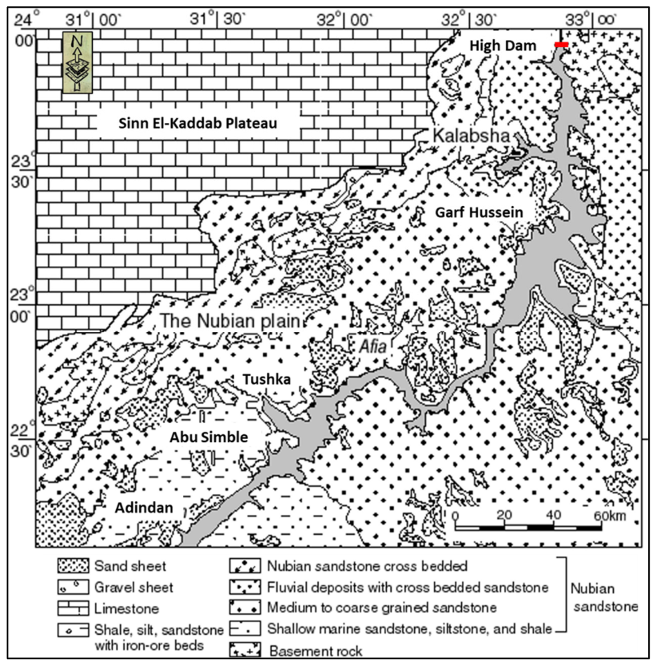
The study area comprises Lake Nasser and the adjacent Tushka Lakes in southern Egypt (Figure 1). Lake Nasser is a large artificial reservoir formed by impounding the Nile River following completion of the Aswan High Dam in the late 1960s [21]. Extending approximately 500 km from southern Egypt into northern Sudan, the lake typically ranges from 10 to 30 km wide. At high operational levels, Lake Nasser stores as much as 1011 m3 of water and inundates several thousand square kilometers, making it Egypt’s primary strategic surface-water storage facility [22]. The hydrogeologic setting of the Lake Nasser region is dominated by the Nubian Sandstone Aquifer System (NSAS), one of the largest fossil aquifers in the world, extending beneath much of southwestern Egypt, southeastern Libya, northeastern Chad, and northern Sudan. In this study area, the aquifer consists of sandstone interbedded with shale and clay, with a total thickness ranging from 390 to 592 m [23]. Hydrogeological investigations indicate that the Nubian Sandstone sequence can be subdivided into several water-bearing layers. These horizons are separated by semi-confining units, with local hydraulic connections through interfingering and facies changes [24]. It consists of sandstone interbedded with shale and clay. Unconfined (shallow) and confined (deep) groundwater conditions are present, and earlier studies have documented hydraulic connectivity between upper and lower aquifer layers in the Lake Nasser region [25,26,27].
Lake Nasser and its surroundings are situated within a hyper-arid desert environment characterized by extremely sparse vegetation, high evaporative demand, and extensive aeolian sand sheets and dune fields, particularly along the northern shoreline [15]. These environmental conditions pose well-known challenges for satellite-based water mapping, including strong land–water spectral contrast, mixed pixels along irregular shorelines, shallow-water and turbidity effects, and spectral confusion with dark soils, wet sand, and shadowed terrain. The surrounding geology consists of Nubian Sandstone plateaus, localized basement rocks, and volcanic outcrops, which influence shoreline morphology and embayment geometry and contribute to spatial variability in shoreline dynamics [21]. The Tushka Lakes are a group of shallow depressional basins found west and southwest of the main Lake Nasser channel. These basins are intermittently connected to Lake Nasser via natural spillways and the topography of the Tushka Depression [5]. During periods of elevated lake levels or exceptional flood events, water spills into the Tushka basins, leading to rapid lake expansion; during drier periods, the basins are partially or completely desiccated. This episodic connectivity, combined with shallow bathymetry and complex shoreline geometry, results in pronounced seasonal and interannual variability in water extent. Consequently, the Tushka Lakes provide a stringent test case for evaluating the performance of spectral water indices under highly dynamic inundation and mixed-shoreline pixels. Together, Lake Nasser and the Tushka Lakes form a coupled surface-water system whose spatial and temporal variability reflects both upstream hydrologic forcing and local geomorphic and hydrogeologic controls. The contrasting behaviors of the stable main reservoir and the highly variable Tushka basins make this region well-suited for comparative evaluation of Landsat-derived water indices and for long-term monitoring of surface-water dynamics in hyper-arid environments.

2.2. Surface and Subsurface Geology

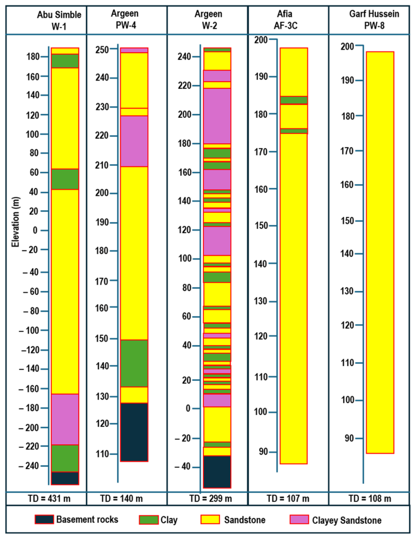
In the Nasser Lake area, the Nubian Sandstone represents a small portion of the well-known Nubian Sandstone Aquifer System in the Eastern Sahara, which covers the entire area of southwest Egypt, southeast Libya, northeast Chad, and northern Sudan and thus constitutes the main source of groundwater in this area (Figure 2 and Figure 3). The aquifer is composed of sandstone intercalated with shale and clay, with a total thickness ranging from 390 to 592 m [23]. The hydrogeology of the study area was studied by several authors [5,28,29,30,31,32,33]. Hydrogeologically, El-Shazly et al. [24] proposed that the sediments comprising the Nubian aquifer system may be subdivided regionally into two or three water-bearing layers, with intervening shale or sandy shale confining units, some of which are hydraulically connected through interfingering and local facies changes. The shallow or upper water-bearing horizons exist under the free water table, while the lower or deeper water-bearing horizons exist under confined conditions. In the lake region, El Ramly [23] noticed a clear hydraulic connection between the upper and lower layers of the Nubian Sandstone aquifer. Subsurface geology of the study area, the west side of Nasser Lake, was inferred from lithological logs of various wells drilled there (Figure 1 and Figure 3 [34]). The Nubian Sandstone aquifer includes water-bearing sands and sandstones, separated by semi-confining clay and sandy-clay intercalations. It directly overlays the basement complex.

3. Data Used

3.1. Remote Sensing Data

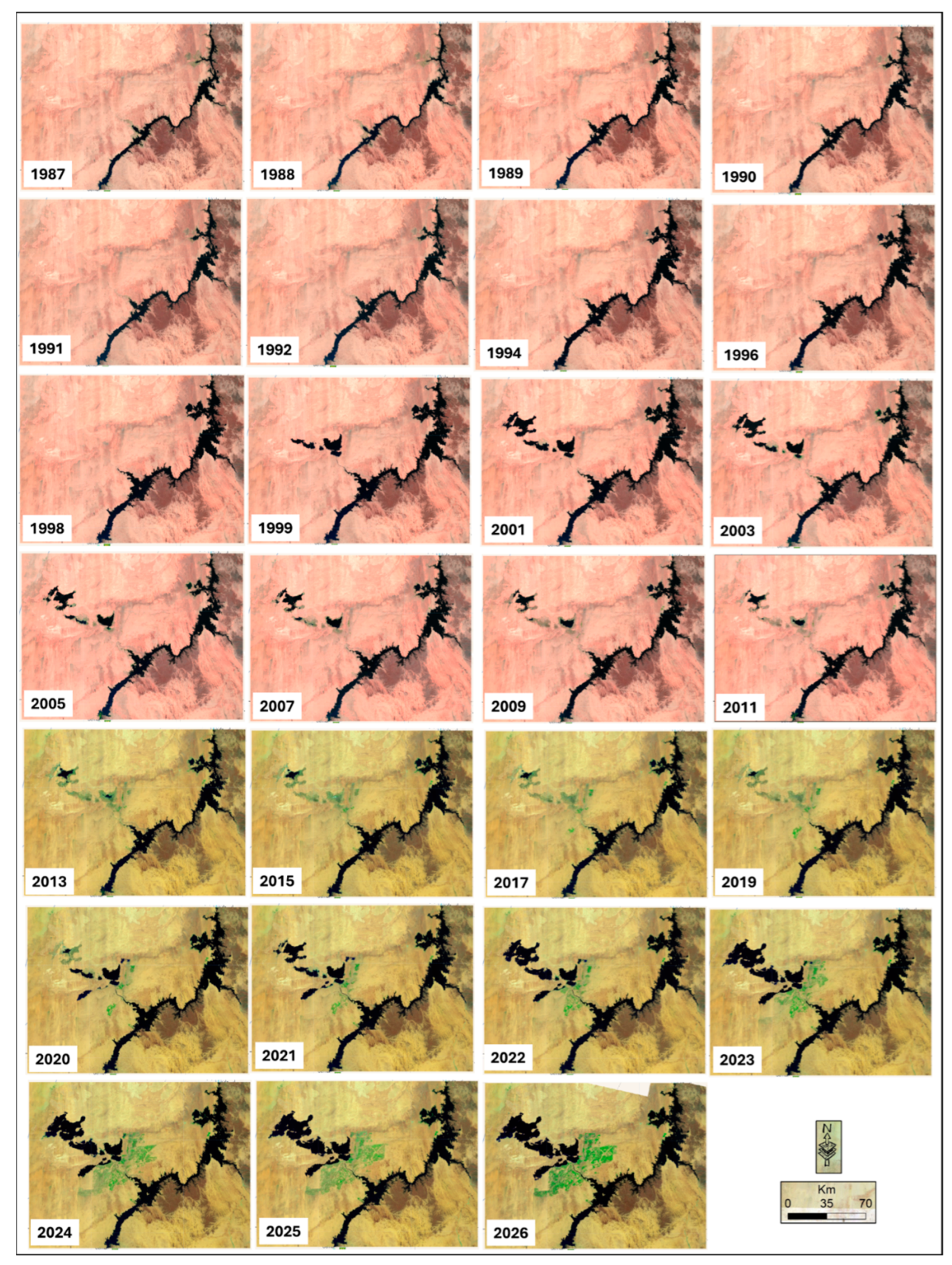
The core dataset used in this study is the Landsat surface reflectance archive, which provides the temporal foundation for evaluating spectral water indices and monitoring long-term surface-water dynamics in Lake Nasser and the Tushka Lakes. The remote-sensing component was designed around a cloud-based analytical workflow implemented in Google Earth Engine (GEE) [17,18], in which all image access, filtering, preprocessing, and multi-temporal analysis were performed. Landsat Collection 2, Tier 1, Level 2 Surface Reflectance (SR) products were selected because they provide radiometrically and geometrically corrected observations appropriate for consistent cross-date analysis [35]. Landsat 5 TM provides the historical record from 1987 to 2013, whereas Landsat 8 OLI provides the post-2013 record. The main spectral difference between the two sensors lies in the positions and widths of their visible, near-infrared, and shortwave-infrared bands; therefore, only spectrally equivalent 30 m bands were used for index calculation. In this study, TM bands 1, 2, 3, 4, 5, and 7 were matched, respectively, to OLI bands 2, 3, 4, 5, 6, and 7 for blue, green, red, NIR, SWIR1, and SWIR2 reflectance. OLI coastal aerosol and cirrus bands were not used in the water-index formulas. Landsat 7 ETM+ was not included in the long-term reconstruction because the scan-line corrector failure after 2003 produces systematic data gaps that complicate shoreline extraction and quarterly compositing; excluding ETM+ also avoided introducing a third sensor transition into the time series. Visible, near-infrared (NIR), and shortwave-infrared (SWIR) bands at 30 m spatial resolution were used because they are required to compute the seven Landsat-derived water indices evaluated in this study. Table 1 summarizes the Landsat datasets and their relevant characteristics, and Figure 4 provides representative images from the time series.
Within the Landsat/GEE workflow, Landsat scenes were filtered to the study area boundary and screened for atmospheric contamination using the quality-assurance information supplied with the Level 2 SR products (QA_PIXEL) [36]. Pixels affected by cloud, cloud shadow, cirrus, or dilated cloud were masked before computing the water indices to improve classification reliability. To support long-term monitoring, the processed imagery was aggregated into quarterly composites (January–March, April–June, July–September, and October–December) using a median reducer, thereby reducing residual cloud effects and providing a temporally consistent basis for seasonal and interannual comparison. This Landsat-based quarterly archive constitutes the primary input for evaluating index performance, selecting the most robust water-extraction approach, and reconstructing long-term surface-water dynamics across the Lake Nasser–Tushka system. Additional preprocessing and analytical details are presented in the Methodology section.

3.2. Observation Wells Data

In addition to the Landsat archive, the study uses supporting hydrogeologic datasets to interpret possible surface–subsurface interactions along the western margin of Lake Nasser. These data include groundwater levels from 44 observation wells (piezometers) distributed across five sectors west of the lake—Garf Hussein, Tushka, Abu Simbel, Adindan, and Argeen (Figure 1 and Table 2). The wells provide a spatial framework for assessing groundwater response relative to long-term changes in surface-water extent. The five monitoring sectors represent different hydrogeologic settings and distances from the High Dam, allowing comparison of hydraulic conditions along the lake margin. The well network includes both shallow and deep piezometers, thereby providing information relevant to vertical and lateral variations in groundwater conditions within the Nubian Sandstone Aquifer System.
To complement the Landsat-based surface-water analysis, daily Lake Nasser stage records for 1965–2014 and monthly groundwater-level measurements from the observation wells were used to evaluate potential lake–aquifer seepage. These records do not replace the remote-sensing data; rather, they provide independent hydrogeologic context for interpreting long-term shoreline behavior and water persistence derived from Landsat. Lithological and hydrogeological information from the drilled wells in each sector was also used to estimate hydraulic conductivity, seepage-face thickness, and hydraulic gradients needed for the Darcy-based seepage calculations. Accordingly, the data used in this study can be grouped into two complementary categories: (1) Landsat imagery processed in Google Earth Engine for water-index evaluation and long-term surface-water monitoring, and (2) lake-stage, piezometric, and hydrogeologic data for supporting interpretation of surface–subsurface interaction in the Lake Nasser–Tushka system.

4. Methodology

The methodology was designed as a Landsat/GEE-based workflow to evaluate water indices and monitor long-term surface-water dynamics in Lake Nasser and the Tushka Lakes. The workflow integrates cloud-based image processing in Google Earth Engine (GEE), multi-index spectral analysis, threshold-based water extraction, accuracy assessment, temporal reconstruction, and hydrogeologic interpretation [19,20]. In sequence, the workflow included (1) acquisition of Landsat Collection 2 Level 2 surface-reflectance imagery for 1987–2026; (2) preprocessing and quality masking using QA_PIXEL; (3) generation of quarterly median composites; (4) computation of seven Landsat-derived water indices (NDWI, EWI, NDX, WRI, AWEInsh, TCW, and NWI); (5) extraction of binary water masks using index-specific thresholds; (6) comparative evaluation of index performance using mapped area and classification accuracy metrics; (7) selection of the most robust index for long-term application; (8) re-construction of quarterly surface-water dynamics and persistence patterns; and (9) qualitative interpretation of potential lake–aquifer seepage using lake-stage, piezometric, and hydrogeologic data.

4.1. Data Preprocessing

Preprocessing was applied to create a temporally consistent Landsat archive suitable for both index evaluation and long-term monitoring. Landsat 5 TM and Landsat 8 OLI Collection 2 Tier 1 Level 2 surface-reflectance imagery were accessed and processed in Google Earth Engine [18]. Scenes were filtered to the Lake Nasser–Tushka study area, and cloud-, cloud-shadow-, cirrus-, and dilated-cloud pixels were removed using the QA_PIXEL quality band [36]. Sensor harmonization was handled at four levels [37,38]. First, both datasets were taken from the same Collection 2 Level 2 surface-reflectance processing framework, so reflectance values were atmospherically corrected and distributed in a comparable scaled-reflectance format. Second, equivalent 30 m spectral bands were renamed to a common band scheme before index computation: blue, green, red, NIR, SWIR1, and SWIR2. Third, all composites were generated on the native 30 m Landsat grid and clipped to the same study-area boundary, ensuring that mapped area was computed from a consistent pixel size. Fourth, the same index equations, thresholding logic, masking procedure, and area-calculation method were applied to both TM and OLI composites. The Landsat 5–Landsat 8 transition was therefore treated as a controlled sensor change rather than a methodological break: the time series ends for TM in 2013, resumes with OLI after its operational availability in 2013, and no artificial adjustment was applied beyond the surface-reflectance harmonization and common-band mapping described above. Landsat 7 ETM+ was excluded from the long-term reconstruction to avoid scan-line corrector gaps after 2003 and to maintain a simpler two-sensor TM–OLI record. Quarterly median composites were then generated for January–March, April–June, July–September, and October–December. This aggregation reduced residual atmospheric contamination, minimized the influence of individual outlier scenes, and provided a consistent seasonal sampling unit for comparing observations before and after the Landsat 5–Landsat 8 sensor transition. Quarters with insufficient valid observations after QA masking, severe residual contamination, or incomplete spatial coverage over the water bodies were treated as poor-quality composites and were not used for quantitative interpretation; where necessary, the nearest valid quarterly or annual observation was used only to preserve temporal context in figures and tables, not to replace the original mapped value. These preprocessed composites formed the base dataset for computing all evaluated water indices and reconstructing long-term surface-water dynamics.

4.2. Spectral Water-Index Computation

A central component of the proposed framework is the comparative evaluation of Landsat-derived spectral water indices for water extraction in a hyper-arid reservoir environment [39,40]. Seven indices were computed from the quarterly Landsat composites: the Normalized Difference Water Index (NDWI) [41]; Equation (1), the normalized difference index (NDX) [42]; Equation (2), the New Water Index (NWI) [43]; Equation (3), the Water Ratio Index (WRI) [44]; Equation (4), the Automated Water Extraction Index (AWEInsh) [45]; Equation (5), the Tasseled Cap Wetness (TCW) transformation [46]; Equation (6); and the Enhanced Water Index (EWI) [47], Equation (7). Each index was calculated using the standard Landsat band formulation after preprocessing. Binary water masks were then produced using an index-specific thresholding procedure consisting of two stages: histogram-guided threshold calibration, followed by the application of a fixed threshold [48]. In the calibration stage, index-value histograms were generated from representative quarterly composites over the study area, the dominant water and non-water modes were identified, and an initial candidate threshold was placed at the local minimum between these modes. Candidate thresholds were then checked against stratified visual reference samples and representative shoreline transects. If a candidate value produced systematic commission errors over dark desert surfaces, wet sand, shadowed terrain, or omission errors over shallow water and mixed shoreline pixels, it was adjusted within the same histogram-defined separation interval. The term “global threshold” therefore refers to the final index-specific threshold selected after this calibration and validation process; it does not mean that a new unconstrained threshold was recalculated independently for every image or quarter. Once selected, the same final threshold and decision rule were applied consistently to all Landsat 5 TM and Landsat 8 OLI quarterly composites to preserve temporal comparability across the multi-decadal record. For indices in which larger values indicate water, pixels equal to or greater than the selected threshold were classified as water; for TCW, pixels greater than the selected wetness threshold were classified as water. Sensor comparability was supported by using Landsat Collection 2 Level 2 surface reflectance products, equivalent spectral bands, a common 30 m grid, identical masking logic, and quarterly median compositing. Mixed and shallow shoreline pixels were not treated as a separate class because the mapping objective was binary water/non-water delineation. Instead, these ambiguous pixels were handled conservatively through threshold calibration, visual reference checks, shoreline transects, and quarterly compositing, and they are explicitly recognized as a principal source of shoreline uncertainty when interpreting the long-term water-area estimates. The goal of this step was not only to extract water but also to determine which index is most robust for long-term monitoring of surface-water dynamics in Lake Nasser and the Tushka Lakes.
N D W I = ( G b 3 N I R b 5 ) ( G b 3 + N I R b 5 )
N D X = ( R b 4 S W I R b 6 ) ( R b 4 + S W I R b 6 )
N W I = ( B b 2 ( N I R b 5 + S W I R b 6 + S W I R b 7 ) ) ( B b 2 + ( N I R b 5 + S W I R b 6 + S W I R b 7 ) )
W R I = ( G b 3 + R b 4 ) ( N I R b 5 + S W I R b 6 )
A W E I n s h = 4 × G b 3 S W I R 1 b 6 0.25   ×   N I R b 5 + 2.75 × S W I R 2 b 7
T C W = 0.0315 × B b 2 + 0.2021 × G b 3 + 0.3102 × R b 4 + 0.1595 × N I R b 5 0.6806 × S W I R 1 b 6 0.6109 × S W I R 2 b 7
E W I = ( G b 3 N I R b 5 S W I R b 6 ) ( G b 3 + N I R b 5 + S W I R b 6 )

4.3. Accuracy Assessment

To evaluate the suitability of each Landsat water index, classification outputs were assessed against reference data derived from visual interpretation of Landsat false-color composites and high-resolution imagery available in Google Earth. Accuracy assessment was performed on the seven index-based water masks using an error matrix approach [49]. A stratified random sample of 1000 reference points was generated to represent the two target classes, water and non-water, while also ensuring coverage of the main temporal, sensor-specific, seasonal, and shoreline conditions encountered in the Lake Nasser–Tushka system. The validation samples were distributed across representative Landsat 5 TM and Landsat 8 OLI composites to include both the historical TM period and the more recent OLI period. Temporal coverage included early, middle, and recent parts of the 1987–2026 record, while seasonal coverage included both high-water and low-water quarters where valid cloud-free or cloud-minimized composites were available. Spatially, the reference points were allocated across persistent open-water areas of Lake Nasser, intermittently inundated Tushka basins, stable dry desert surfaces, wet or recently exposed sediments, and mixed shoreline zones. Attention was given to shoreline buffers, shallow margins, narrow embayments, and wet-sand transition zones because these areas are the main sources of classification uncertainty in hyper-arid reservoir environments. For each point, the mapped class from the index-based classification was compared with the manually assigned reference class, and the resulting confusion matrix was used to compute producer’s accuracy, user’s accuracy, overall accuracy, and Cohen’s kappa coefficient [50]. These metrics provide the quantitative basis for comparing index performance and identifying the most reliable method for subsequent long-term application within the Landsat/GEE workflow.
PA   ( % ) = X t X b × 100
UA   ( % ) = X t X a × 100
Overall   accuracy   ( OA ) = 1 N p = 1 c n i
Kappa   coefficient   ( Ka ) = N p = 1 c X t p = 1 c ( X a   .   X b ) N 2 p = 1 c ( X a   .     X b )
where N stands for the total number of pixels, c for the number of classes, xt for the total number of pixels in row “p” and column “p,” xa for the total number of samples in row “p,” and xb for the total number of samples in column “p” in the error matrix.

4.4. Comparative Evaluation

The evaluated methods were compared using two complementary criteria: (1) mapped surface-water area and its absolute and percentage difference among indices, and (2) classification accuracy statistics derived from the error matrix. This comparative step was designed to identify the index that best balances spatial realism, quantitative agreement, and transferability across the multi-decadal Landsat archive. Indices showing minimal area deviation, together with high overall accuracy and strong kappa agreement, were considered more suitable for long-term monitoring. On this basis, the index with the most stable and interpretable performance in the Lake Nasser–Tushka environment was selected for full time-series reconstruction and persistence mapping.

4.5. Trend Analysis (Mann–Kendall and Sen’s Slope)

Monotonic trends in the NDWI-derived surface-water record were evaluated using the non-parametric Mann–Kendall (MK) test and Sen’s slope estimator [51,52]. The datasets analyzed were the mapped water-area time series for three spatial units: Lake Nasser, the Tushka Lakes, and the combined Lake Nasser–Tushka surface-water system. The input values were derived from the binary NDWI water masks produced from the Landsat composites. For 1987–1997, annual observations were used due to the lower temporal density of usable scenes in the early archive, whereas for 1998–2026, quarterly observations were used to retain seasonal information. For trend testing, quarterly values were also aggregated to an annual mean surface-water area, where a single long-term monotonic trend was required, thereby reducing the influence of intra-annual seasonality. The MK test was applied to determine the direction and statistical significance of monotonic trends without assuming normality, and Sen’s slope was used to estimate the median rate of change in the mapped area through time. Statistical significance was evaluated at α = 0.05. Results were interpreted separately for Lake Nasser, the Tushka Lakes, and the total water area because these units differ strongly in hydrologic behavior and temporal variability.

4.6. Seepage Estimation from Lake Nasser to the Nubian Sandstone Aquifer (Darcy’s Law)

The workflow also incorporates a supporting hydrogeologic component to interpret possible lake–aquifer interaction. Seepage losses from Lake Nasser to the Nubian Sandstone Aquifer were estimated for the western shoreline using a hydraulic-gradient approach based on Darcy’s law. The analysis used (i) daily lake-stage observations for 1965–2014, which were aggregated to annual mean lake levels; (ii) monthly groundwater heads from 44 observation wells distributed across five sectors (Garf Hussein, Tushka, Abu Simbel, Adindan, and Argeen), which were aggregated to representative annual heads for each sector; and (iii) sector-specific hydrostratigraphic information, including lithologic logs, aquifer thickness, and hydraulic-conductivity estimates. For each sector and year, seepage discharge was calculated as Q = KIA, where Q is seepage discharge, K is hydraulic conductivity, I is the hydraulic gradient between the lake and groundwater observation point, and A is the effective seepage cross-sectional area. The hydraulic gradient was estimated as I = Δh/L, where Δh is the difference between the annual mean lake level and the representative groundwater head, and L is the approximate horizontal flow-path distance from the lake margin to the observation well or well group. The effective seepage area was approximated as A = B × W, where B is the saturated aquifer thickness or hydraulically active seepage thickness and W is the representative shoreline length assigned to each sector. The resulting values provide sector-scale approximations rather than direct flux measurements, calibrated groundwater model outputs, or closed-water-budget terms.
The Darcy-based estimates require several simplifying assumptions. First, flow was treated as predominantly lateral from the lake toward the adjacent Nubian Sandstone Aquifer along representative shoreline-to-well flow paths. Second, hydraulic conductivity within each sector was assumed to be representative of the permeable units intersected by the observation wells, although local heterogeneity due to shale and clay interbeds is expected. Third, the effective seepage area was estimated from the sectoral shoreline length and the saturated aquifer thickness, rather than measured directly. Fourth, hydraulic gradients were derived from contemporaneous lake-stage and representative groundwater-head differences normalized by assumed flow-path length. Finally, the estimates were interpreted as potential seepage under the measured hydraulic conditions, not as calibrated groundwater model outputs. This approach treats seepage primarily as lateral flow through permeable shoreline sediments driven by stage–head differences and provides a complementary hydrogeologic context for interpreting long-term surface-water persistence and shoreline behavior derived from the Landsat analysis.
The seepage component is therefore included as complementary hydrogeologic context for interpreting possible surface–subsurface interaction, rather than as direct quantitative confirmation of lake–aquifer exchange. The Darcy-based estimates are sector-scale, assumption-dependent approximations and should not be interpreted as direct measurements, calibrated groundwater-model outputs, or closed water-budget terms. Because the seepage dataset ends in 2014 and only partially overlaps the Landsat-derived surface-water record, comparisons between estimated seepage and mapped water persistence are qualitative and hypothesis-generating. Establishing quantitative lake–aquifer exchange would require additional field measurements, spatial correlation analysis, water-budget closure, tracer evidence, and calibrated groundwater-flow modeling.

5. Results

5.1. Remote Sensing Results (Landsat/GEE)

5.1.1. Statistical Evaluation of Water-Extraction Indices

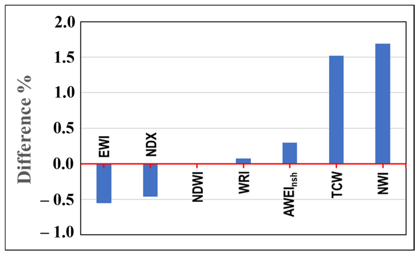
The first set of results addresses the evaluation of Landsat-derived water indices within the Landsat/GEE workflow. Index performance was assessed using mapped surface-water area (km2), absolute and percentage area difference relative to the NDWI classification, and classification metrics derived from the error matrix (overall accuracy and Cohen’s kappa). As summarized in Table 3 and Figure 5, all tested indices could separate water from non-water across most of the study scene, but their performance differed along shallow shorelines and spectrally complex land–water boundaries. These differences are especially important in the Lake Nasser–Tushka system, where mixed pixels, dark desert surfaces, and variable inundation create a demanding test environment for long-term water mapping.
Figure 5. Comparison of water-extraction models based on the percent area difference relative to the reference classification (NDWI) (red line). For each spectral index, the plotted value represents. Negative values indicate that an index mapped less water than NDWI, while positive values indicate over-mapping relative to NDWI. The figure summarizes the relative agreement among indices and complements the accuracy statistics reported in Table 4.
Earth 07 00112 g005
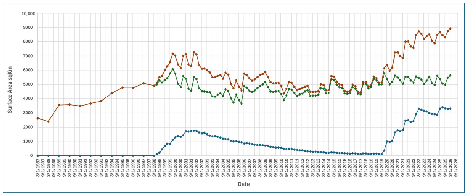
Table 4. Surface area changes with time for Tushka lakes, Lake Nasser, and the total water surface.
Date
(m/y)
Tushka Lakes (km2)Nasser Lake
(km2)
Total Water
(km2)
Date
(m/y)
Tushka Lakes
(km2)
Nasser Lake
(km2)
Total Water
(km2)
Date
(m/y)
Tushka Lakes
(km2)
Nasser Lake
(km2)
Total Water
(km2)
12/198702631263110-12/20051016.94286.1530304-06/2016155.64337.84493.4
12/198802411241101-03/2006975.23877.8485307-09/2016140.84398.64539.4
12/198903544354404-06/2006932.23630.8456310-12/2016169.14814.74983.8
12/199003579357907-09/20068614895575601-03/2017158.54714.14872.6
12/199103485348510-12/2006886.64775.4566204-06/2017129.44360.34489.7
12/199203656365601-03/2007861.54568.5543007-09/2017120.64323.64444.2
12/199303819381904-06/20078004466526610-12/2017157.75014.75172.4
12/199404405440507-09/2007769.94580.1535001-03/2018153.55025.65179.1
12/199504779477910-12/20077504750550004-06/2018129.74730.44860.1
12/199604772477201-03/2008754.24907.8566207-09/2018132.448344966.4
12/199705076.25076.204-06/2008730.64999.4573010-12/2018153.45390.95544.3
01-03/199804920.84920.807-09/20087005173587301-03/2019150.55283.75434.2
04-06/19981204995.75115.710-12/2008697.54802.5550004-06/2019126.44992.55118.9
07-09/19982205280.25500.201-03/20096304527515707-09/2019123.95010.95134.8
10-12/1998442.25140.35582.504-06/2009596.54480.5507710-12/20193705778.16148.1
01-03/1999680.35330.56010.807-09/2009571.34528.7510001-03/2020991.453836374.4
04-06/1999846.45430.6627710-12/20095744550512404-06/2020955.85003.85959.6
07-09/1999815.25770.36585.501-03/2010553.34349.7490307-09/202010155169.46184.4
10-12/19991111.56060.77172.204-06/2010484.63887.4437210-12/20201616.55631.97248.4
01-03/20001276.25766.8704307-09/2010467.64232.4470001-03/20211770.35486.87257.1
04-06/20001369.35052.7642210-12/2010491.84704.2519604-06/20211716.15292.57008.6
07-09/20001324.34827.66151.901-03/2011484.74634.3511907-09/202118005047.36847.3
10-12/20001421.95585.1700704-06/20114304410484010-12/20212468.75532.98001.6
01-03/20011720.15405.57125.607-09/2011400.24189.8459001-03/20222486.85517.88004.6
04-06/20011700.34714.7641510-12/20113804308468804-06/20222378.15289.77667.8
07-09/20011730.54559.5629001-03/2012374.74375.3475007-09/20222435.65121.97557.5
10-12/20011741.75516.3725804-06/20123224528485010-12/20222920.15556.48476.5
01-03/20021738.65375.4711407-09/2012314.84585.2490001-03/20233282.45458.18740.5
04-06/20021612.34740.7635310-12/20123004200450004-06/20233220.95340.58561.4
07-09/20021566.34538.7610501-03/2013269.142184487.107-09/20233153.35034.18187.4
10-12/200216004520612004-06/2013276.84216.14492.910-12/20233100.45275.38375.7
01-03/200315004500600007-09/2013255.14274.34529.401-03/20243000.55514.78515.2
04-06/200314004450585010-12/2013260.54747.75008.204-06/20242941.75092.28033.9
07-09/20031359.14151.9551101-03/2014246.14717.74963.807-09/20242915.24975.97891.1
10-12/20031373.14126.9550004-06/2014203.64391.94595.510-12/20242862.65611.38473.9
01-03/20041328.34271.7560007-09/2014198.44415.34613.701-03/20253288.45390.28678.6
04-06/20041263.94394.1565810-12/2014235.45346.6558204-06/20253386.45060.58446.9
07-09/20041198.44211.6541001-03/2015231.953195550.907-09/20253303.84991.18294.9
10-12/20041169.64658.4582804-06/2015207.94988.25196.110-12/20253273.15471.48744.5
01-03/20051145.34553.7569907-09/2015192.94799.34992.201-03/20263288.45634.68923
04-06/20051038.14002.9504110-12/2015185.14771.44956.5
07-09/20051003.73736.3474001-03/2016174.343814555.3
Among the evaluated indices, NDWI, EWI, NDX, and WRI yielded the strongest overall performance, showing small area deviations and high classification agreement. NDWI produced the highest overall accuracy (93.6%) and kappa (0.898), with a zero relative area difference because it served as the reference, whereas EWI achieved 92.7% overall accuracy and 0.851 kappa. NDX and WRI also performed well, indicating that several Landsat formulations can delineate open water reliably in this environment. By contrast, TCW and NWI showed larger mapped-area deviations and weaker agreement statistics, indicating greater sensitivity to shoreline mixing and spectrally confusing non-water targets. Overall, the comparative results demonstrate that index choice has a measurable influence on the mapped extent of water and therefore directly affects the reliability of long-term surface-water reconstruction.

5.1.2. Selection of an Index for Long-Term Time-Series Mapping

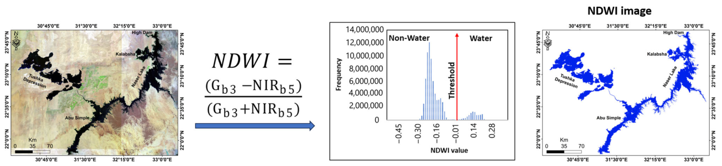
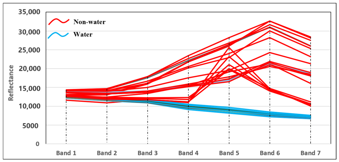
A key outcome of the Landsat-based evaluation is the selection of NDWI as the primary index for long-term monitoring. This choice was based on a multi-criteria interpretation rather than a single metric. NDWI provided a particularly strong balance of high classification agreement, stable shoreline delineation, simple formulation, and practical transferability across the multi-sensor Landsat archive. In the context of a long-term monitoring workflow, these characteristics are essential because the selected index must remain interpretable, reproducible, and robust across varying hydrologic conditions and across both TM and OLI imagery. The workflow shown in Figure 6 illustrates how each spectral index was converted into a binary water mask, while Figure 7 provides the spectral basis for water–non-water discrimination in the Lake Nasser–Tushka environment.
NDWI is the most suitable index for this study because it offers the basis for monitoring long-term surface-water dynamics in a hyper-arid reservoir setting. Its performance reflects the strong contrast between water in the green and near-infrared bands, which remains effective in a landscape dominated by dry sand, bare rock, and sparse vegetation. Quarterly compositing in Google Earth Engine further improves the temporal stability of NDWI-based mapping by reducing residual cloud and atmospheric effects. The results, therefore, show that the value of the workflow lies not simply in computing multiple indices but in identifying the one most appropriate for consistent multi-decadal monitoring. On this basis, NDWI was carried forward to reconstruct quarterly surface-water dynamics in Lake Nasser and the Tushka Lakes from 1987 to 2026.

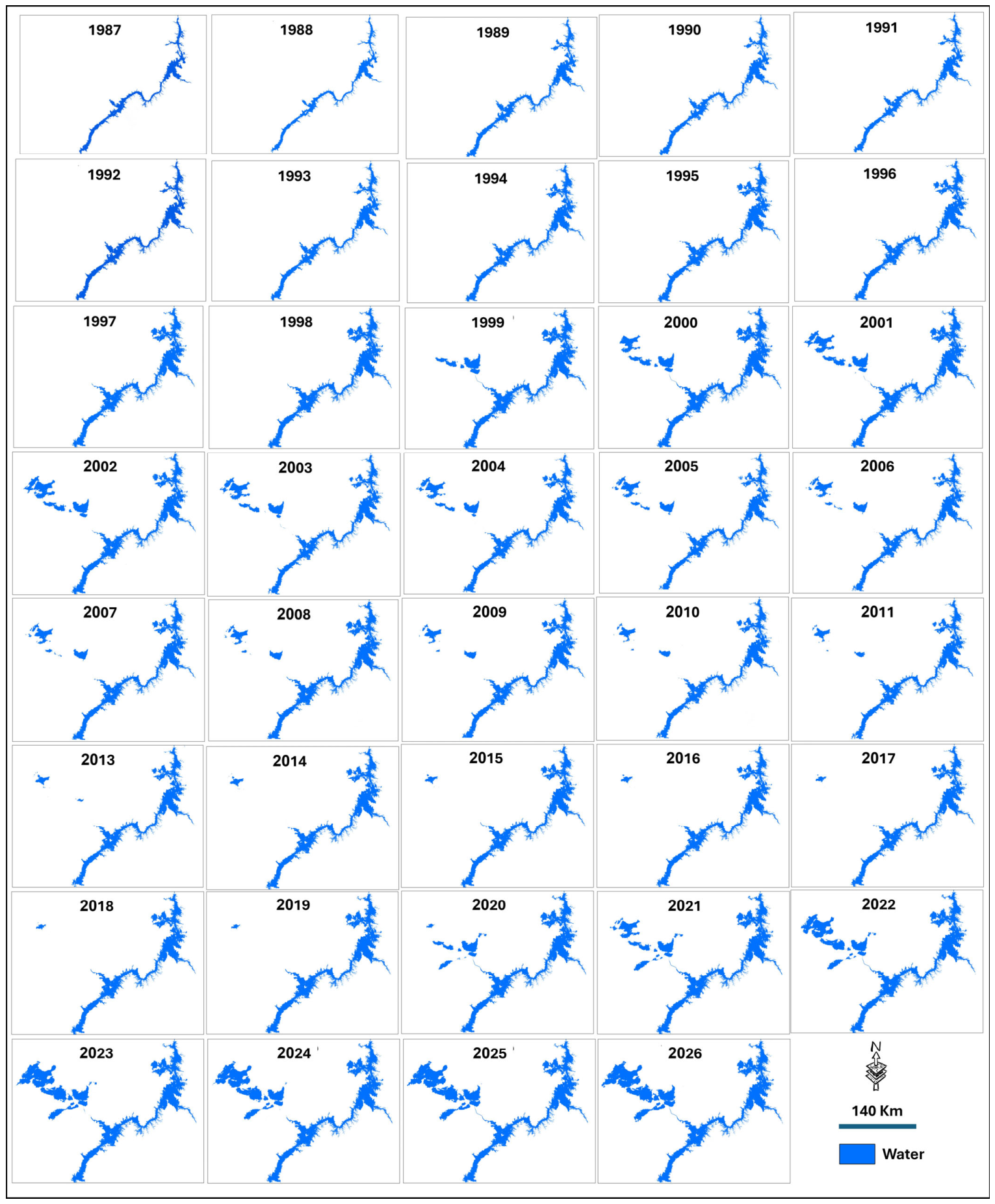
5.1.3. Time-Series Analysis of NDWI (1987–2026)

Application of NDWI to the quarterly Landsat composites produced a multi-decadal record of surface-water dynamics for Lake Nasser, the Tushka Lakes, and their combined water surface from 1987 to 2026 (Figure 8 and Table 4). Rather than simply reflecting a single regional water-level signal, the record reveals two distinct hydrologic behaviors. Lake Nasser serves as the stable core of the system: its mapped area changes over time, but large parts of the central and southern reservoir remain persistently inundated due to greater water depth, longitudinal continuity, and sustained connection to the main Nile reservoir. In contrast, the Tushka basins function as shallow peripheral storage zones, with their surface-water extent responding disproportionately to relatively small changes in lake stage. Once water spills into these low-relief depressions, large horizontal expansions can occur; during drawdown, the same shallow geometry promotes rapid contraction and partial desiccation. The NDWI time series, therefore, indicates that the spatial differences between Lake Nasser and Tushka are controlled not only by total water availability but also by basin morphology, connectivity thresholds, and shoreline slope (Figure 9).
The persistence and trend results refine this interpretation by separating stable inundation from episodic shoreline migration. High-persistence zones in Lake Nasser represent areas where water occurrence is controlled primarily by reservoir storage and channel depth, whereas low-persistence zones along northern margins and within the Tushka basins mark areas where small vertical changes in stage translate into large areal changes. These low-persistence zones are also the most sensitive to mixed pixels and threshold uncertainty, because the mapped shoreline often coincides with shallow water, wet sand, and intermittently exposed sediment. Consequently, the long-term record should be interpreted as a robust indicator of seasonal-to-interannual water-area dynamics rather than as an exact instantaneous shoreline inventory. The Mann–Kendall and Sen’s slope analyses add value by distinguishing broad monotonic tendencies from short-term fluctuations, but the most important hydrologic insight is the persistent contrast between a relatively buffered main reservoir and highly responsive peripheral basins.

5.2. Hydrogeologic (Piezometer) and Seepage Results

Piezometer Data Analysis

The hydrogeologic results provide a complementary, but necessarily more uncertain, interpretation of possible lake–aquifer exchange along the western shoreline. Darcy-based seepage estimates for Garf Hussein, Tushka, Abu Simbel, Adindan, and Argeen indicate spatial heterogeneity rather than a uniform leakage pattern. Garf Hussein shows the largest estimated seepage magnitudes, whereas Abu Simbel shows the lowest, with intermediate values in the remaining sectors. This pattern is consistent with spatial differences in hydraulic gradient, shoreline geometry, aquifer thickness, and the distribution of permeable sandstone units relative to shale and clay interbeds. However, these values should be read as sector-scale potential flux estimates, not direct measurements of seepage. Their magnitude depends strongly on assumed hydraulic conductivity, representative flow-path length, effective seepage area, and the degree to which observation wells capture local head conditions near the lake shoreline.
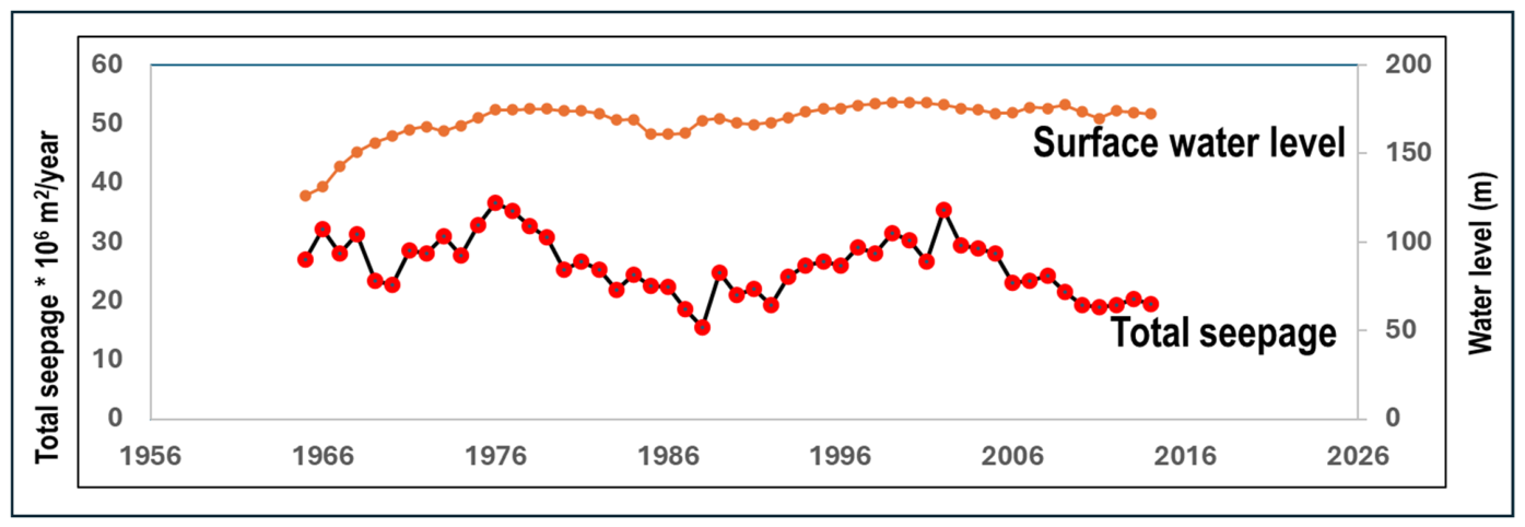
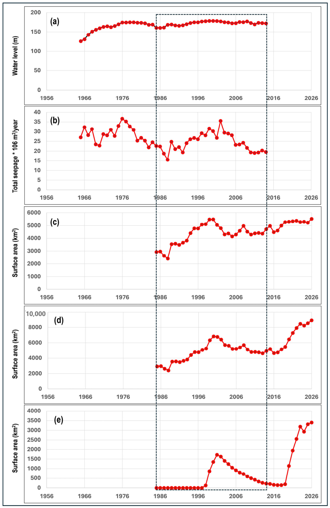
The relation between lake stage and estimated seepage is therefore best interpreted as a hydraulic tendency rather than a calibrated causal model. Higher lake levels increase the potential head difference between the reservoir and adjacent aquifer, which can increase estimated seepage where permeable pathways are present (Table 5, Figure 10). At the same time, local lithologic heterogeneity, delayed groundwater response, vertical leakage between aquifer layers, uncertainty in lake-margin geometry, and uncertainty in hydraulic conductivity can weaken or obscure a simple stage–seepage relationship. The calculated annual seepage values range from 15.58 × 10⁶ to 36.68 × 10⁶ m3/year. In addition, the seepage record ends in 2014, whereas the Landsat-based water-area record extends to 2026. Therefore, only the 1987–2014 overlap period supports qualitative comparison between surface-water extent and seepage estimates. When considered alongside the NDWI persistence maps, the seepage estimates help identify sectors where lake–aquifer exchange is more likely, but they do not independently establish the magnitude of recharge, post-2014 seepage behavior, or detailed flow pathways.

6. Discussion

6.1. Implications of the Surface-Water Record

The discussion confirms that the main contribution of this study lies in the development of a Landsat/GEE-based workflow for evaluating Landsat water indices and applying the most suitable index to monitor long-term surface-water dynamics in Lake Nasser and the Tushka Lakes. The comparative results demonstrate that water mapping in this hyper-arid reservoir environment is strongly influenced by shoreline complexity, mixed pixels, and spectrally confusing dry-land surfaces. In this setting, NDWI proved to be the most suitable index for long-term application because it maintained high agreement with the reference data while also providing stable and interpretable shoreline delineation across the multi-sensor Landsat archive. This outcome is important because the reliability of any long-term surface-water record depends first on selecting a method that remains robust across changing conditions and across decades of imagery.
From a methodological perspective, the Google Earth Engine workflow offers a practical way to transform large Landsat archives into a consistent monitoring product. By integrating cloud-based preprocessing, QA-based masking, quarterly compositing, multi-index calculation, threshold-based water extraction, and accuracy evaluation into a single analytical environment, the workflow reduces technical barriers to long-term reservoir analysis and improves reproducibility. The quarterly compositing strategy is especially useful in the Lake Nasser–Tushka system because it suppresses atmospheric noise and residual cloud contamination while preserving the seasonal-to-interannual variability needed for long-term interpretation. At the same time, quarterly aggregation can smooth very short-lived inundation events, so the mapped series should be interpreted as representative seasonal conditions rather than exact instantaneous shoreline positions.
The long-term NDWI record is most informative when interpreted in terms of system behavior rather than as a sequence of mapped areas. Lake Nasser and the Tushka Lakes respond differently because they occupy different geomorphic and hydraulic settings. The main reservoir has a relatively continuous water body and deeper basin geometry, so changes in stage are expressed mainly as shoreline adjustment around a persistent water core. The Tushka basins, by contrast, are shallow depressions connected by spillways and topographic lows; once connectivity thresholds are crossed, water can spread rapidly across broad, low-gradient surfaces, and when levels fall, those areas recede just as rapidly. This explains why the Tushka record contains sharper expansions and contractions than Lake Nasser, even though both are part of the same regional surface-water system. The persistence maps, therefore, provide hydrologic interpretation by identifying where water occurrence is structurally stable and where it is threshold-controlled and episodic.
More broadly, the findings suggest that the proposed Landsat/GEE workflow can serve as a transferable approach for monitoring other large desert reservoirs and inland basins, provided that local index evaluation is performed before long-term implementation. Because index behavior is landscape-dependent, this study reinforces the conclusion that no single spectral water index should be assumed optimal without site-specific testing. In that sense, the broader value of this work lies not only in the resulting Lake Nasser–Tushka record itself, but also in the demonstration that a combination of Landsat water-index evaluation, cloud-based processing, and multi-decadal surface-water reconstruction can provide a reliable basis for environmental monitoring in hyper-arid settings.

6.2. Implications for Potential Groundwater Recharge

Although the primary emphasis of the study is Landsat water-index evaluation and long-term surface-water dynamics, the hydrogeologic observations add important supporting context for interpreting the surface-water record. Groundwater levels in the Nubian Sandstone Aquifer adjacent to Lake Nasser and the Tushka Lakes can be discussed in relation to the NDWI-derived maps of surface-water extent and persistence, but these links should be interpreted cautiously. NDWI is an optical indicator of surface-water presence and does not directly measure recharge, seepage flux, or hydraulic connectivity. Accordingly, the discussion of groundwater response in this study is best understood as an interpretation supported by independent piezometric and seepage information, rather than as a direct output of the remote-sensing analysis itself.
When interpreted alongside groundwater observations, the persistence maps indicate areas where sustained surface-water presence may create conditions favorable to lake–aquifer interaction, but this interpretation must be treated with caution. Longer inundation duration can maintain hydraulic gradients for longer periods, yet persistence alone does not demonstrate seepage, recharge, or a causal hydraulic connection. Darcy-based calculations are highly sensitive to hydraulic conductivity, which can vary by orders of magnitude in interbedded sandstone, shale, and clay sequences. They are also affected by assumptions about saturated thickness, effective seepage area, shoreline length, flow direction, and the distance over which hydraulic gradients are calculated. Because these parameters are represented at the sector scale, the estimates cannot resolve local preferential pathways, vertical leakage, delayed aquifer response, or spatially variable bank-storage effects. Thus, any spatial coincidence between persistent surface water and estimated seepage should be treated only as evidence of possible association, not as proof of a specific recharge rate, seepage pathway, or causal mechanism.
The Tushka Lakes are especially important for interpreting uncertainty because they combine shallow bathymetry, intermittent hydraulic connection, and spectrally complex wet shorelines. Their rapid expansion during high-water periods does not necessarily imply equivalent groundwater recharge, because part of the mapped increase may represent shallow surface spreading over low-permeability or fine-grained deposits. Conversely, rapid contraction may reflect evaporation, disconnection from the main reservoir, infiltration, or some combination of these processes. The NDWI record identifies the timing and spatial footprint of these changes, but it cannot separate the relative contributions of evaporation, infiltration, seepage, bank storage, and reservoir operation. This distinction strengthens the interpretation of Figure 11: the apparent agreement among water-level, surface-water-area, and seepage estimates should be viewed only as qualitative covariation. Without formal spatial correlation, calibrated groundwater-flow modeling, water-budget closure, tracer evidence, or independent field validation, the magnitude, direction, and mechanism of lake–aquifer exchange remain uncertain.
Overall, the integrated results show that this study’s strongest contribution is not simply documenting that water extent changed over time but explaining how different parts of the Lake Nasser–Tushka system respond differently to the same broad hydrologic forcing. NDWI-based mapping provides a consistent long-term record of surface-water persistence and variability, while the seepage analysis offers a first-order hydrogeologic context for interpreting possible surface–subsurface exchange. The seepage estimates should therefore be used as interpretive indicators rather than definitive water-budget terms. Future work should reduce uncertainty by combining the Landsat-derived persistence record with field-based hydraulic-head monitoring, aquifer tests, geophysical characterization of shoreline sediments, tracer studies, and calibrated groundwater-flow models. Such integration would allow the spatial patterns identified here to be translated into more quantitative estimates of recharge, seepage pathways, and storage impacts.

6.3. Environmental Problems Associated with High Water Levels in the River Nile

High water levels in the River Nile and its associated systems (e.g., irrigation canals, drains, and large reservoirs such as Lake Nasser) could result in various environmental issues. The main routes and typical examples can be summarized as follows: (1) Floodwater inundation of low-lying floodplains can result in crop damage, delay planting/harvesting, and deposit fine sediments clogging soil pores or covering seedlings. Example: inundation of agricultural fields and adjacent settlements in the Nile Valley and Delta during high-stage events, with subsequent sediment deposition and cleanup needs [53]. (2) Sediment derived from floods can settle in canals, reducing their conveyance capacity and increasing maintenance needs. Example: silt and debris buildup in secondary canals following flood events can impair irrigation delivery and drainage efficiency [53]. (3) Inundation of wastewater facilities, waste dumps, or contaminated soils can mobilize nutrients, pathogens, and metals into surface waters. Example: floodwater transport of heavy-metal-contaminated materials from wastewater disposal areas toward canals and the Nile, thereby increasing downstream environmental and health risks [54]. (4) Enhanced flow velocity and shear stress may favor erosion of alluvial banks, resulting in bank retreat, loss of vegetation, and localized damage of embankments and riverside infrastructure. Example: erosion hotspots at bends where cohesive bank materials are undercut during sustained high stage [55]. (5) Rapid water-level rise inundates exposed shores; repeated wetting–drying and wave action can destabilize sediments and increase turbidity through resuspension. Example: erosion and sediment remobilization along the Lake Nasser shorelines during rapid stage changes, thereby raising nearshore turbidity [56]. (6) A sustained high river stage can elevate adjacent groundwater tables. Waterlogging reduces aeration in the root zone and can depress yields, while evaporation in arid/semi-arid climates concentrates salts at the surface, worsening soil salinity. (7) Floods transport more suspended sediments, nutrients, and organic matter. Decomposition of flooded biomass and high organic loading can increase biochemical oxygen demand and cause localized low-oxygen conditions (i.e., severe waterlogging and salinization reported in parts of the northeastern Nile Delta, associated with shallow saline groundwater and constraints on irrigation water quality [57,58]), particularly in weakly mixed areas. Example: Surveys of Lake Nasser show seasonal contrasts (pre- and post-flood) in nutrient and chlorophyll dynamics indicative of flood-driven material inputs and changes in productivity [56,59,60]. (8) Standing water in depressions, canals and drains can expand mosquito breeding habitat and increase exposure to microbial contamination where sanitation is compromised. Example: stagnant pools that persist after inundation events may increase vector abundance and increase waterborne disease risk [53]. Overall, these examples illustrate that high Nile water levels are not only a flooding hazard; they can also drive geomorphic change, soil and groundwater degradation, and impacts on water quality and health across the connected river–canal–reservoir system. In the Lake Nasser–Tushka setting, these processes are particularly relevant along shallow shorelines and intermittently inundated zones, where stage changes can rapidly modify sediment and water quality conditions.

7. Future Trends and Study Limitations

Future work should build directly on this study’s three central components: the Landsat/GEE workflow, the evaluation of Landsat water indices, and the monitoring of long-term surface-water dynamics in Lake Nasser and the Tushka Lakes. First, the workflow can be expanded through multi-sensor integration by combining Landsat with higher-temporal-frequency optical observations, such as Sentinel-series imagery, to improve detection of short-lived inundation events and rapid shoreline shifts, especially in the Tushka basins. Second, future studies may extend the index-evaluation component by testing adaptive thresholds, machine learning classifiers, or sensor-specific calibration strategies to determine whether water extraction can be made more robust under highly variable illumination, turbidity, and mixed-pixel conditions. Third, the long-term monitoring component can be strengthened through near-real-time implementation in cloud platforms such as Google Earth Engine, allowing routine updates of quarterly or monthly water extent products for water resource assessment and operational reservoir management. In addition, coupling the mapped water record with elevation–area–volume relationships would allow future work to move beyond surface-water area toward more complete estimates of storage variability.
Several limitations should be considered when interpreting the results. First, the mapped water masks are derived from 30 m Landsat imagery, so shoreline position and area estimates remain sensitive to mixed pixels, narrow embayments, and irregular coastlines. Second, the use of quarterly composites improves temporal consistency but can smooth short-duration inundation peaks or abrupt contractions, particularly in episodically connected parts of the Tushka system. Third, the comparative evaluation of indices relies on visually interpreted reference data rather than fully contemporaneous field-based shoreline observations, introducing unavoidable uncertainty into the accuracy assessment. Fourth, the monotonic trend analysis captures broad tendencies in the time series but may be influenced by temporal aggregation, serial correlation, seasonality, and abrupt operational changes. Finally, the seepage analysis contains important methodological and temporal limitations. Darcy-based estimates are highly sensitive to hydraulic conductivity, hydraulic gradient, seepage thickness, shoreline length, and the assumed flow-path distance; these parameters were represented at the sector scale rather than resolved locally. In addition, seepage calculations end in 2014 because the lake-stage and groundwater datasets used for this component do not extend to 2026, whereas Landsat surface-water monitoring continues through 2026. As a result, the 1987–2014 overlap period supports only qualitative comparison between seepage and mapped water extent, while post-2014 Landsat observations should be interpreted only as surface-water dynamics and not as evidence of quantified seepage. This study’s primary contribution, therefore, remains the remote-sensing analysis; the seepage component is complementary, uncertainty-bearing, and hypothesis-generating. Despite these limitations, this study provides a strong and reproducible basis for future refinement of index selection and long-term surface-water monitoring in large desert reservoirs.

8. Conclusions

This study developed a Landsat/GEE-based workflow to evaluate water indices and monitor long-term surface-water dynamics in Lake Nasser and the Tushka Lakes, Egypt, using Landsat 5 TM and Landsat 8 OLI surface reflectance imagery from 1987 to 2026. By integrating Google Earth Engine processing, multi-index comparison, threshold-based water extraction, and temporal analysis, the workflow provided a consistent basis for assessing which Landsat-derived index is most suitable for water mapping in a hyper-arid reservoir environment characterized by shallow shorelines, mixed pixels, and spectrally complex dry-land backgrounds. The analysis evaluated seven spectral water indices and used 1000 stratified reference samples to quantify classification performance.
The comparative evaluation showed that several indices performed well, but NDWI provided the best balance of classification accuracy, mapped-area consistency, interpretability, and transferability across the multi-sensor Landsat archive. NDWI achieved the highest classification statistics in the evaluation scene, with an overall accuracy of 93.6% and a kappa coefficient of 0.898. NDWI mapped 8935.7 km2 of water in the comparison scene and served as the reference for mapped-area consistency; NDX and WRI differed from NDWI by only −0.46% and 0.073%, respectively, whereas TCW and NWI showed larger deviations of 1.52% and 1.69%. NDWI was therefore selected as the most robust option for long-term use because it provided reliable shoreline delineation and consistent performance throughout the study period. These findings highlight that the main value of the workflow lies not only in computing multiple water indices, but in identifying the one most suitable for reproducible multi-decadal monitoring.
Application of NDWI to quarterly Landsat composites from 1987 to 2026 generated a multi-decadal record of surface-water behavior that clearly distinguishes the relatively stable core reservoir of Lake Nasser from the more episodic and highly dynamic Tushka Lakes. The mapped total water area increased from 2631 km2 in 1987 to 8923 km2 in early 2026. Lake Nasser ranged from a minimum mapped area of 2411 km2 in 1988 to a maximum of 6060.7 km2 in late 1999, whereas the Tushka Lakes expanded from no mapped water before 1998 to more than 3300 km2 during 2025. The results show broad zones of persistent water in the central and southern sectors of Lake Nasser, in contrast to strong seasonal and interannual variability in the shallow Tushka basins. Persistence mapping and time-series analysis further demonstrate that the most dynamic water–land transitions occur along intermittently inundated shorelines, emphasizing the importance of using a carefully evaluated index for long-term monitoring in such environments.
The hydrogeologic analysis adds complementary interpretive value by placing mapped persistence and shoreline behavior in the context of possible lake–aquifer seepage along the western margin of Lake Nasser. However, this component should be interpreted as an uncertainty-bearing, sector-scale hydrogeologic interpretation rather than as direct quantitative confirmation of lake–aquifer exchange. The Darcy-based estimates are assumption-dependent and do not represent direct seepage measurements, calibrated groundwater model outputs, or closed water budget terms. The present study therefore identifies only qualitative co-variation between persistent surface water, lake stage, groundwater observations, and estimated seepage during the period of data overlap, but it does not demonstrate causality, quantify post-2014 seepage behavior, or resolve detailed flow pathways. Establishing a quantitative lake–aquifer exchange relationship would require additional spatial correlation analysis, calibrated groundwater modeling, water-budget closure, tracer or field-based validation, and higher-resolution hydraulic monitoring. Taken together, the results demonstrate that Google Earth Engine processing, Landsat water-index evaluation, and multi-decadal surface-water reconstruction provide a strong and reproducible foundation for monitoring large desert reservoirs, while the seepage component should be viewed as complementary, hypothesis-generating hydrogeologic context to guide future validation. This study therefore contributes both a site-specific understanding of the Lake Nasser–Tushka system and a transferable workflow that can support future remote-sensing and hydrogeologic investigations in other arid and semi-arid surface-water systems.

Author Contributions

Conceptualization, B.A.E.-H., A.M.Y., A.R., S.R. and E.-S.M.R.; methodology, B.A.E.-H. and A.M.Y.; software, A.M.Y., A.R. and S.R.; validation, B.A.E.-H., A.M.Y. and E.-S.M.R.; investigation, B.A.E.-H., A.M.Y., A.R. and S.R.; resources, A.R., S.R. and E.-S.M.R.; formal analysis, B.A.E.-H. and A.M.Y.; data curation, B.A.E.-H., S.R. and E.-S.M.R.; writing—original draft preparation, B.A.E.-H., A.M.Y. and S.R.; writing—review and editing, B.A.E.-H., A.M.Y. and E.-S.M.R.; visualization, B.A.E.-H., A.M.Y., A.R., S.R. and E.-S.M.R.; supervision, B.A.E.-H., A.M.Y. and E.-S.M.R. All authors have read and agreed to the published version of the manuscript.

Funding

This research received no external funding.

Institutional Review Board Statement

Not applicable.

Informed Consent Statement

Not applicable.

Data Availability Statement

The data supporting the conclusions of this article will be made available upon request. Data is contained within the article.

Conflicts of Interest

The authors declare no conflicts of interest.

References

  1. Teixeira, A.M.D.E.; Batista, L.V.; da Silva, R.M.; Freitas, L.M.T.; Santos, C.A.G. Dynamic monitoring of surface area and water volume of reservoirs using satellite imagery, computer vision and deep learning. Remote Sens. Appl. Soc. Environ. 2024, 35, 101205. [Google Scholar] [CrossRef]
  2. Abegeja, D. The application of satellite sensors, current state of utilization, and sources of remote sensing dataset in hydrology for water resource management. J. Water Health 2024, 22, 1162–1179. [Google Scholar] [CrossRef]
  3. Che, L.; Li, S.; Liu, X. Improved surface water mapping using satellite remote sensing imagery based on optimization of the Otsu threshold and effective selection of remote-sensing water index. J. Hydrol. 2025, 654, 132771. [Google Scholar] [CrossRef]
  4. Chipman, J.W. A Multisensor Approach to Satellite Monitoring of Trends in Lake Area, Water Level, and Volume. Remote Sens. 2019, 11, 158. [Google Scholar] [CrossRef]
  5. Elewa, H.H. Water resources and geomorphological characteristics of Tushka and west of Lake Nasser, Egypt. Hydrogeol. J. 2006, 14, 942–954. [Google Scholar] [CrossRef]
  6. Muala, E.; Mohamed, Y.A.; Duan, Z.; Van der Zaag, P. Estimation of Reservoir Discharges from Lake Nasser and Roseires Reservoir in the Nile Basin Using Satellite Altimetry and Imagery Data. Remote Sens. 2014, 6, 7522–7545. [Google Scholar] [CrossRef]
  7. Ahmed, M.; Abdelrehim, R.; Elshalkany, M.; Abdrabou, M. Impacts of the Grand Ethiopian Renaissance Dam on the Nile River’s downstream reservoirs. J. Hydrol. 2024, 633, 130952. [Google Scholar] [CrossRef]
  8. Abdelhady, A.A.; Samy-Kamal, M.; Ismail, E.; Hussain, A.M.; Gamvroula, D.E.; Ali, A.; Ahmed, M.S.; Abdel-Raheem, K.H.M.; Saibi, H.; Sami, M.; et al. Climate warming and mismanagement drive the shift of fish communities in the Wadi El-Rayan arid lakes. Water 2024, 16, 2685. [Google Scholar] [CrossRef]
  9. Donchyts, G.; Baart, F.; Winsemius, H.; Gorelick, N.; Kwadijk, J.; van de Giesen, N. Earth’s surface water change over the past 30 years. Nat. Clim. Change 2016, 6, 810–813. [Google Scholar] [CrossRef]
  10. Wulder, M.A.; Roy, D.P.; Radeloff, V.C.; Loveland, T.R.; Anderson, M.C.; Johnson, D.M.; Healey, S.; Zhu, Z.; Scambos, T.A.; Pahlevan, N.; et al. Fifty years of Landsat science and impacts. Remote Sens. Environ. 2022, 280, 113195. [Google Scholar] [CrossRef]
  11. Dritsas, E.; Trigka, M. Advances in geospatial artificial intelligence for remote sensing applications. Comput. Sci. Rev. 2026, 60, 100913. [Google Scholar] [CrossRef]
  12. Miura, Y.; Shamsudduha, M.; Suppasri, A.; Sano, D. A Global Multi-Sensor Dataset of Surface Water Indices from Landsat-8 and Sentinel-2 Satellite Measurements. Sci. Data 2025, 12, 1253. [Google Scholar] [CrossRef] [PubMed]
  13. Wulder, M.A.; Loveland, T.R.; Roy, D.P.; Crawford, C.J.; Masek, J.G.; Woodcock, C.E.; Allen, R.G.; Anderson, M.C.; Belward, A.S.; Cohen, W.B.; et al. Current status of Landsat program, science, and applications. Remote Sens. Environ. 2019, 225, 127–147. [Google Scholar] [CrossRef]
  14. Chen, J.; Wang, Y.; Wang, J.; Zhang, Y.; Xu, Y.; Yang, O.; Zhang, R.; Wang, J.; Wang, Z.; Lu, F.; et al. The performance of Landsat-8 and Landsat-9 data for water body extraction based on various water indices: A comparative analysis. Remote Sens. 2024, 16, 1984. [Google Scholar] [CrossRef]
  15. Abd Ellah, R.G. Morphometric analysis of Toshka Lakes in Egypt: A succinct review of geographic information systems and remote sensing based techniques. Egypt. J. Aquat. Res. 2021, 47, 215–221. [Google Scholar] [CrossRef]
  16. Bhunia, G.S. Assessment of automatic extraction of surface water dynamism using multi-temporal satellite data. Earth Sci. Inform. 2021, 14, 1433–1446. [Google Scholar] [CrossRef]
  17. Google Earth Engine Data Catalog. Landsat Collections in Earth Engine; Google Developers. 2026. Available online: https://developers.google.com/earth-engine/datasets/catalog/landsat/ (accessed on 2 February 2026).
  18. Gorelick, N.; Hancher, M.; Dixon, M.; Ilyushchenko, S.; Thau, D.; Moore, R. Google Earth Engine: Planetary-scale geospatial analysis for everyone. Remote Sens. Environ. 2017, 202, 18–27. [Google Scholar] [CrossRef]
  19. Lan, L.; Wang, Y.-G.; Chen, H.-S.; Gao, X.-R.; Wang, X.-K.; Yan, X.-F. Improving on mapping long-term surface water with a novel framework based on the Landsat imagery series. J. Environ. Manag. 2024, 353, 120202. [Google Scholar] [CrossRef]
  20. Jahangeer, J.; Joshi, P.; Kapoor, A.; Tang, Z. A review of AI-driven Google Earth Engine applications in surface water monitoring, assessment, and management. Discov. Geosci. 2025, 3, 140. [Google Scholar] [CrossRef] [PubMed]
  21. Embabi, N.S. Lake Nasser Region. In Landscapes and Landforms of Egypt; Springer: Cham, Switzerland, 2018. [Google Scholar] [CrossRef]
  22. Elhaddad, H.; Sultan, M.; Yan, E.; Abdelmohsen, K.; Mohammad, A.T.; Badawy, A.; Karimi, H.; Saleh, H.; Emil, M.K. Optimization of floodwater redistribution from Lake Nasser could recharge Egypt’s aquifers and mitigate its excessive floods. Commun. Earth Environ. 2024, 5, 385. [Google Scholar] [CrossRef]
  23. El Ramly, I.M. Geomorphology, Hydrogeology, Planning for Groundwater Resources and Land Reclamation in Lake Nasser Region and Its Environs; Technical Report; Desert Research Institute: Cairo, Egypt, 1973. [Google Scholar]
  24. El-Shazly, E.M.; Aly, M.A.; High Dam Authority. Hydrological conditions and seepage processes in the Lake Nasser region, southern Egypt. In High Dam Authority Technical Report; High Dam Authority: Cairo, Egypt, 1977. [Google Scholar]
  25. Wafa, T.A.; Labib, A.H. Seepage losses from Lake Nasser. In Man-Made Lakes: Their Problems and Environmental Effects; Ackermann, W.C., White, G.F., Worthington, E.B., Ivens, J.L., Eds.; Stony Brook Foundation: Stony Brook, NY, USA, 1973; Volume 17, pp. 287–291. [Google Scholar] [CrossRef]
  26. Hamdan, A.M.; Selim, S.A.; Abdallah, M.M. Interactions between the surface water and groundwater in the western shoreline of Lake Nasser, Upper Egypt. Arab. J. Geosci. 2013, 6, 77–84. [Google Scholar] [CrossRef]
  27. Aly, M.M.; Sakr, S.A.; Fayad, S.A.K. Evaluation of the impact of Lake Nasser on the groundwater system in Toshka under future development scenarios, Western Desert, Egypt, Arab. J. Geosci. 2019, 12, 553. [Google Scholar] [CrossRef]
  28. Selim, S.A. Hydrogeological Studies and Seepage Evaluation of the Nubian Sandstone Aquifer Adjacent to Lake Nasser, Southern Egypt. Master’s Thesis, Faculty of Science, Assiut University, Assiut, Egypt, 1986. [Google Scholar]
  29. Tamer, A.M.; El-Shazly, M.M.; Elewa, H.H. Hydrogeological Characteristics of the Nubian Sandstone Aquifer System in the Lake Nasser Region, Egypt; Egyptian Geological Surve: Cairo, Egypt, 1987. [Google Scholar]
  30. Sherief, Y.A.; Ahmed, S.A. Groundwater-surface water interaction along the Lake Nasser shoreline, southern Egypt. J. Afr. Earth Sci. 1990, 10, 589–602. [Google Scholar]
  31. Mousa, S.M. Seepage and Hydraulic Connectivity Between Lake Nasser and the Adjacent Nubian Sandstone Aquifer. Ph.D. Dissertation, Cairo University, Cairo, Egypt, 1991. [Google Scholar]
  32. Kim, J.; Sultan, M. Assessment of the long-term hydrologic impacts of Lake Nasser and related irrigation projects in southwestern Egypt. J. Hydrol. 2002, 262, 68–83. [Google Scholar] [CrossRef]
  33. Yan, P.; Zhang, Y. Information extraction of water systems in semi-arid regions using the enhanced water index. Remote Sens. Inf. 2007, 6, 62–67. [Google Scholar]
  34. CONOCO. Geological Map of Egypt, NF 36 NW El Sad El Ali; Scale 1:500,000; Egyptian General Petroleum Corporation: Cairo, Egypt, 1987. [Google Scholar]
  35. U.S. Geological Survey. Landsat Collection 2 Level-2 Science Products; Fact Sheet 2021–3055; U.S. Geological Survey: Reston, VA, USA, 2021. [CrossRef]
  36. U.S. Geological Survey. Landsat Collection 2 Quality Assessment Bands (QA_PIXEL); U.S. Geological Survey: Reston, VA, USA, 2022.
  37. Pahlevan, N.; Lee, Z.; Wei, J.; Schaaf, C.B.; Schott, J.R.; Berk, A. On-orbit radiometric characterization of OLI (Landsat-8) for applications in aquatic remote sensing. Remote Sens. Environ. 2014, 154, 272–284. [Google Scholar] [CrossRef]
  38. Roy, D.P.; Kovalskyy, V.; Zhang, H.K.; Vermote, E.F.; Yan, L.; Kumar, S.S.; Egorov, A. Characterization of Landsat-7 to Landsat-8 reflective wavelength and normalized difference vegetation index continuity. Remote Sens. Environ. 2016, 185, 57–70. [Google Scholar] [CrossRef] [PubMed]
  39. Zhai, K.; Wu, X.; Qin, Y.; Du, P. Comparison of surface water extraction performances of different classic water indices using OLI and TM imagery. Geo-Spat. Inf. Sci. 2015, 18, 32–42. [Google Scholar] [CrossRef]
  40. Yang, X.; Chen, Y.; Wang, J. Combined use of Sentinel-2 and Landsat 8 to monitor water surface area dynamics using Google Earth Engine. Remote Sens. Lett. 2020, 11, 687–696. [Google Scholar] [CrossRef]
  41. McFeeters, S.K. The use of the normalized difference water index (NDWI) in the delineation of open water features. Int. J. Remote Sens. 1996, 17, 1425–1432. [Google Scholar] [CrossRef]
  42. Rogers, A.S.; Kearney, M.S. Reducing signature variability in unmixing coastal marsh Thematic Mapper scenes using spectral indices. Int. J. Remote Sens. 2004, 25, 2317–2335. [Google Scholar] [CrossRef]
  43. Jiang, H.; Feng, M.; Zhu, Y.; Lu, N.; Huang, J.; Xiao, T. An Automated Method for Extracting Rivers and Lakes from Landsat Imagery. Remote Sens. 2014, 6, 5067–5089. [Google Scholar] [CrossRef]
  44. Shen, L.; Li, C. Water body extraction from Landsat ETM+ imagery using AdaBoost algorithm. In Proceedings of the 18th International Conference on Geoinformatics; IEEE: Piscataway, NJ, USA, 2010; pp. 1–4. [Google Scholar] [CrossRef]
  45. Feyisa, G.L.; Meilby, H.; Fensholt, R.; Proud, S.R. Automated water extraction index: A new technique for surface water mapping using Landsat imagery. Remote Sens. Environ. 2014, 140, 23–35. [Google Scholar] [CrossRef]
  46. Crist, E.P. A TM tasseled cap equivalent transformation for reflectance factor data. Remote Sens. Environ. 1985, 17, 301–306. [Google Scholar] [CrossRef]
  47. Purnam, K.K.; Prasad, A.D.; Ganasala, P. Water indices for surface water extraction using geospatial techniques: A brief review. Sustain. Water Resour. Manag. 2024, 10, 70. [Google Scholar] [CrossRef]
  48. Ji, L.; Zhang, L.; Wylie, B. Analysis of dynamic thresholds for the normalized difference water index. Photogramm. Eng. Remote Sens. 2009, 75, 1307–1317. [Google Scholar] [CrossRef]
  49. Foody, G.M. Status of land cover classification accuracy assessment. Remote Sens. Environ. 2002, 80, 185–201. [Google Scholar] [CrossRef]
  50. Cohen, J. A coefficient of agreement for nominal scales. Educ. Psychol. Meas. 1960, 20, 37–46. [Google Scholar] [CrossRef]
  51. Mann, H.B. Nonparametric tests against trend. Econometrica 1945, 13, 245–259. [Google Scholar] [CrossRef]
  52. Sen, P.K. Estimates of the regression coefficient based on Kendall’s tau. J. Am. Stat. Assoc. 1968, 63, 1379–1389. [Google Scholar] [CrossRef]
  53. FAO. Flood Management and Preparedness in the Near East and North Africa Region; Food and Agriculture Organization of the United Nations: Rome, Italy, 2021. [Google Scholar]
  54. El-Haddad, B.A.; Youssef, A.M.; Rizk, S. Flood and heavy metal risks from wastewater site in Sohag Governorate, Egypt: Integrating hydrological modeling and mapping. Environ. Earth Sci. 2026, 85, 173. [Google Scholar] [CrossRef]
  55. Ahmed, A.A.; Fawzi, A. Meandering and bank erosion of the River Nile and its environmental impact on the area between Sohag and El-Minia, Egypt. Arab. J. Geosci. 2011, 4, 1–11. [Google Scholar] [CrossRef]
  56. Goher, M.E.; Napiórkowska-Krzebietke, A.; Aly, W.; El-Sayed, S.M.; Tahoun, U.M.; Fetouh, M.A.; Hegab, M.H.; Haroon, A.M.; Sabae, S.A.; Abdel-Aal, E.I.; et al. Comprehensive insight into Lake Nasser environment: Water quality and biotic communities-A case study before operating the Renaissance Dam. Water 2021, 13, 2195. [Google Scholar] [CrossRef]
  57. Arnous, M.O.; Green, D.R. Monitoring and assessing waterlogged and salt-affected areas in the Eastern Nile Delta region, Egypt, using remotely sensed multi-temporal data and GIS. Environ. Monit. Assess. 2015, 187, 431. [Google Scholar]
  58. Hagage, M.; Abdulaziz, A.M.; Elbeih, S.F.; Hewaidy, A.G.A. Monitoring soil salinization and waterlogging in the northeastern Nile Delta linked to shallow saline groundwater and irrigation water quality. Sci. Rep. 2024, 14, 27838. [Google Scholar] [CrossRef] [PubMed]
  59. Abdel-Aal, E.I.; Haroon, A.M.; Ibrahim, S.M.; Abd El-Aziz, G.S.; Sabae, S.A.; Gaber, K.M.; Goher, M.E. Ecological status of Lake Nasser khors, Egypt, before operating the Grand Ethiopian Renaissance Dam. Stoch. Environ. Res. Risk Assess. 2023, 37, 1229–1245. [Google Scholar]
  60. Rizk, R.; Juzsakova, T.; Cretescu, I.; Rawash, M.; Sebestyén, V.; Kovács, Z.; Domokos, E.; Rédey, Á.; Shafik, H. Environmental assessment of physical-chemical features of Lake Nasser, Egypt. Environ. Sci. Pollut. Res. 2020, 27, 20136–20148. [Google Scholar] [CrossRef]
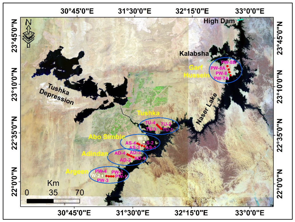
Figure 1. Location of the study area showing Lake Nasser and the adjacent Tushka Lakes in southern Egypt (extending toward northern Sudan). The map provides geographic context for the Landsat-based analysis and highlights the main surface-water bodies evaluated for index performance and long-term monitoring. In addition, observation wells (red circles and white boxes) in five areas (blue ellipses) are superimposed on the image.
Earth 07 00112 g001
Figure 2. Geological map of Lake Nasser and adjacent areas showing the distribution of major lithological units that control shoreline morphology and hydrogeologic conditions.
Earth 07 00112 g002
Figure 3. Representative lithological logs of observation wells from different sectors around Lake Nasser, illustrating variations in the Nubian Sandstone Aquifer stratigraphy across the study area. Well locations are shown in Figure 1.
Earth 07 00112 g003
Figure 4. Example Landsat false-color composites used in this study to illustrate the multi-sensor time series over the Lake Nasser–Tushka region: Landsat 5 TM (1987–2011), displayed as RGB 5–4–3 (SWIR1–NIR–Red); and Landsat 8 OLI (2013–2026), displayed as RGB 7–5–3 (SWIR2–NIR–Green). These composites highlight the water–land contrast in the hyper-arid setting and provide representative scenes from the Landsat archive for computing indices and mapping time series.
Earth 07 00112 g004
Figure 6. Landsat/GEE analytical workflow is used to evaluate Landsat water indices and generate binary surface-water masks. The workflow begins with Landsat Collection 2 Level 2 surface reflectance preprocessing in Google Earth Engine, including study-area filtering, QA_PIXEL cloud- and shadow-masking, and quarterly compositing. Seven spectral water indices were then computed from harmonized Landsat bands, followed by index-specific threshold selection using histogram separation and visual reference checks. The resulting binary masks were compared using mapped water area, relative area difference, and accuracy statistics derived from reference samples. This workflow provides the basis for selecting NDWI for long-term surface-water reconstruction and highlights where uncertainty may enter the analysis, particularly during threshold selection and shoreline classification.
Earth 07 00112 g006
Figure 7. Representative Landsat surface-reflectance signatures for water and non-water targets in the Lake Nasser–Tushka study area. The curves illustrate the spectral contrast between open water, dry desert surfaces, and shoreline/mixed pixels across visible, near-infrared, and shortwave-infrared bands. Strong absorption by water in the NIR and SWIR regions explains why indices using these bands are effective for open-water extraction, whereas overlapping between shallow water, wet sand, and dark desert surfaces helps explain classification uncertainty along complex shorelines. The figure, therefore, provides a spectral basis for interpreting the comparative index results and for selecting NDWI for long-term monitoring.
Earth 07 00112 g007
Figure 8. NDWI-derived surface-water area time series for the Tushka Lakes, Lake Nasser, and the combined water surface (yearly composites, 1987–2026). Values represent mapped surface-water area (km2) computed from the binary NDWI water mask for each Landsat composite after cloud and cloud-shadow masking using QA_PIXEL. The plot summarizes multi-decadal variability in mapped surface-water extent and provides a visual basis for interpreting differences in stability between Lake Nasser and the more episodically inundated Tushka basins.
Earth 07 00112 g008
Figure 9. Continuation of the NDWI-derived quarterly surface-water area time series (1987–2026) for Lake Nasser (green), the Tushka Lakes (blue), and the combined surface-water area (brown). Values represent mapped water area (km2) computed from the binary NDWI mask for yearly from 1987 to 1997 and quarterly from 1998 to 2026 for Landsat composite after cloud and cloud-shadow masking.
Earth 07 00112 g009
Figure 10. The relation between the water level of Nasser Lake and the total seepage loss (m3/year) from 1965 up to 2014 at Nasser Lake. Note: * indicates that seepage values are scaled by a factor of 106.
Earth 07 00112 g010
Figure 11. Potential surface–subsurface interaction in the Lake Nasser–Tushka system. (a) Water level of Lake Nasser between 1965 and 2014. (b) Darcy-based seepage capacity estimated for wells west of Lake Nasser between 1965 and 2014. Note: * indicates that seepage values are scaled by a factor of 106. (c) Lake Nasser surface-area variations between 1985 and 2026. (d) Surface-area variations of Lake Nasser and the Tushka Lakes between 1985 and 2026. (e) Tushka Lakes surface-area variations between 1985 and 2026. The hydrogeologic record and Landsat record overlap only during 1987–2014; therefore, comparisons between seepage and mapped surface-water area are qualitative and limited to this period. Landsat observations after 2014 extend the surface-water monitoring record but do not provide quantified estimates of seepage.
Earth 07 00112 g011
Table 1. Description and characteristics of Landsat time-series data (1987–2026).
Satellite Sensor
and Seams
Spatial Resolution (m)Bands of Interest/Range (Micrometers)Bandwidth
(Micrometers)
Launch Date and Revisit Time
Landsat-5
Landsat 5, level 2, collection 2, tier 1
30Band 1 Visible Blue(0.450–0.520 µm)Launched 1 March 1984
Revisit time 16 days
Band 2 Visible Green(0.520–0.600 µm)
Band 3 Visible Red(0.630–0.690 µm)
Band 4 Near-Infrared(0.760–0.900 µm)
Band 5 Near-Infrared(1.550–1.750 µm)
Band 6 Thermal(10.40–12.50 µm)
Band 7 Mid-Infrared(2.080–2.350 µm)
Landsat-8 OLI
Landsat 8, level 2, collection 2, tier 1
30Band 1 Coastal Aerosol(0.430–0.450 µm)Launched 11 February 2013
Revisit time 16 days
Band 2 Blue(0.450–0.510 µm)
Band 3 Green(0.530–0.590 µm)
Band 4 Red(0.640–0.670 µm)
Band 5 Near-Infrared(0.850–0.880 µm)
Band 6 SWIR 1(1.57–1.65 µm)
Band 7 SWIR 2(2.11–2.29 µm)
Table 2. Elevation and total depth of the piezometers around Nasser Lake.
RegionObservation WellsGround Elevation (m)Total Depth (m)
Garf HusseinPW-7193.8102
PW-8196.1107.6
PW-8A197.3101
PW-8B190.4100
TushkaTU-1187.1100
TU-2197.998.0
TU-3199.9111
TU-4210.8125
W5 deep225.1386
Abu SimbleAS-1188.398.4
AS-2185.695.0
AS-3193.2101
AS-4198.3108
W4 DEEP188.6431
AdindanADW-1180.582.0
ADW-2195.597.0
ADW-3212.9114.6
ADW-4239.1140.1
W3 DEEP245.5390.3
ArgeenPW-1187.7100
PW-2204.9105
PW-3219.3120
PW-4237.5140
W2 DEEP244.5299
Table 3. Statistical comparison of the evaluated water-extraction indices.
Index
Number
Water
Extraction Techniques
Water Area (km2)Area Difference
Based on the NDWI Method (km2)
% Difference
Based on the NDWI Method
Overall Accuracy
%
Kappa
Index
1NDWI8935.70093.60.898
2EWI8942.2−49.9−0.5592.70.851
3WRI8915.96.50.07390.90.831
4NDX8983.4−41.2−0.4690.10.829
5AWELnsh8992.126.30.29589.30.799
6TCW8808.3133.91.5288.40.794
7NWI8793.7148.51.6983.90.773
Table 5. Water-level and total-seepage calculations for the western side of Lake Nasser.
YearTotal Seepage × 106 m3/YearLake Level (Average in m)YearTotal Seepage × 106 m3/YearLake Level (Average in m)
196527.07126.28199021.07167.3
196632.29131.29199122.05166.46
196728.16142.90199219.36167.72
196831.3151.10199324.08170.53
196923.44156.18199426.1173.63
197022.83159.83199526.73175.21
197128.67163.63199626.08175.45
197228.05165.17199729.13177.37
197330.94162.85199828.06178.13
197427.79165.75199931.56178.91
197532.97170.09200030.25178.88
197636.68174.83200126.79178.76
197735.27174.86200235.56177.66
197832.7175.35200329.46175.62
197930.91175.26200429174.86
198025.35174.22200528.13172.79
198126.8174.13200623.19173.10
198225.34172.66200723.4176.20
198321.93169.01200824.28175.62
198424.54169.34200921.64177.66
198522.65160.90201019.37173.59
198622.38161.08201119.06169.93
198718.74161.66201219.29174.14
198815.58168.82201320.33173.23
198924.77169.79201419.56172.43
Disclaimer/Publisher’s Note: The statements, opinions and data contained in all publications are solely those of the individual author(s) and contributor(s) and not of MDPI and/or the editor(s). MDPI and/or the editor(s) disclaim responsibility for any injury to people or property resulting from any ideas, methods, instructions or products referred to in the content.