Illegal Abandoned Waste Sites (IAWSs): A Multi-Parametric GIS-Based Workflow for Waste Management Planning and Cost Analysis Assessment

Abstract

The occurrence of illegal waste activities is a worldwide problem, due to improper actions and inadequate services across many territories. Geographical Information Systems (GISs) software plays a crucial role in optimizing waste management and determining the shortest route paths for waste transportation. This work focuses on the development of a GIS-based workflow for the detection of Illegal Abandoned Waste Sites (IAWSs) and waste management planning. The integration of remote/ground sensing activities, geospatial data, and models within a GIS framework is a useful practice for conducting cost analysis and supporting the development of efficient waste management plans. Firstly, available satellite images are employed in a baseline assessment, combining ancillary and remote sensing data. As a result of satellite monitoring, a ground-piloted survey is carried out by checking the potential-IAWSs density map retrieved from the satellite pre-recognition phase. Hence, a total of 171 ground points are geo-localized and spatialized, according to qualitative on-site products and 2.5D volume analysis. Consequently, distances from illegal dumping sites to proper disposal plants are calculated, achieving the shortest route paths as geospatial information. From these data, a Functional Unit (FU) of 1 ton of mixed waste plus 381.6 kg of inert material is determined, a fundamental stage for comparing different cost analysis processes in similar contexts. By using a GIS-based workflow, a cost analysis assessment is provided, aiming to support principal activities such as waste transportation and disposal to the proper plant (e.g., landfill or incineration). In conclusion, spatial data analysis results are fundamental in managing illegal abandoned waste sites, helping to establish a cost analysis assessment.

1. Introduction

In recent years, the world’s growing population, urban sprawl, and consequent increase in industrial activity have contributed to a rise in waste generation [1]. It is acknowledged that the waste sector is the third largest emitter of methane, after the agricultural and energy sectors [2]. Inadequate waste management has damaging effects on both human health and on the environment, resulting in the contamination of soil, water, and air [3]. Moreover, the presence of unauthorized dumping locations is widely acknowledged as a global problem [4,5]. Swift urban expansion and population increases are considered key factors contributing to the proliferation of illegal abandoned waste, giving rise to environmental risks and safety issues [6]. Hence, a deeper comprehension of the environmental impacts caused by illegal disposal has led innovations in the field of land monitoring. Accordingly, Remote Sensing (RS) and Geographic Information Systems (GISs) are increasingly utilized to assess, monitor, and manage environmental irregularities, especially in the waste dumping context [7]. The new constellation of Very High Resolution (VHR) satellites, along with the development of robust data processing algorithms, can support scientific research and enable exciting new results. In addition, empirical studies and practical experience have proved the usefulness of GIS applications and RS technologies in the detection of illegal waste sites [8]. Therefore, the application of these technologies can facilitate the collection, management, and visualization of relevant data in a geospatial context, improving the objective assessment of environmental data and potential health risks [9,10,11,12,13,14]. Furthermore, sensors applied on satellites and Unmanned Aerial Vehicles (UAVs) can improve the quality of environmental analysis at the local scale, reducing costs and time-consuming activities [15]. GIS technology can also play a crucial role in optimizing waste management by identifying the shortest transportation routes from the point of origin to the final disposal site [16,17,18]. Thus, efficient route planning is essential to minimize travel time, fuel consumption, and costs. Furthermore, considering such outputs, Life Cycle Assessment (LCA) can be a useful tool to evaluate additional waste-to-energy solutions, including cost analysis within the broader waste management planning context. In this regard, GIS-based transport systems can provide the easiest, fastest, and shortest routes by using, for instance, Dijkstra’s algorithm [19]. GIS-based cost analysis represents a crucial step towards the evaluation of optimal solutions for abandoned-waste management by examining geospatial variables for final management costs [20].

Illegal abandoned waste sites require the application of a multidisciplinary approach for the environmental characterization, recognition, and management of damaged sites. For the achievement of these objectives, disciplines such as geomatics, computer science, engineering, and economics have been integrated.

In the end, ancillary, satellite, and ground data are used to investigate areas characterized by the occurrence of illegal abandonment of waste material. During operational processes, GIS-based tools can achieve results for companies that support municipalities and regions, ensuring continuous and reliable environmental monitoring. The implementation of a computerized system for the identification of abandoned waste sites is proposed, aiming to improve effectiveness in territorial monitoring and management. Indeed, the innovative goal of this work is to develop a novel approach capable of identifying and managing IAWSs across the territory using open-source software. Moreover, this study presents an integrated method for assessing the cost analysis and managing illegal abandoned waste sites, combining GIS technologies, remote sensing analysis, field surveys, material analysis, and economic modeling. Hence, the novelty of this work lies in the following steps:

-

Use of open-source software (e.g., QGIS 3.42.1 ‘Münster’, Bizagi Modeler 4.1);

-

Integration of satellite data to optimize ground surveys;

-

Product and volume analysis;

-

Application of algorithms to define optimal routes for waste collection and transportation.

These elements enable more efficient and sustainable waste management planning, providing valuable decision-support tools for environmental policies.

GIS for Waste Management Planning

Waste collection, transport, and disposal are complex processes involving the management of domestic, industrial, and other types of waste. Effective waste management relies on the integration of various technologies, such as remote sensing, proximal sensing, ground-based sensing, Geographic Information Systems (GIS), and related plugins [12,16,17,18,19,20,21,22]. A key objective in this domain is to achieve cost-effectiveness by classifying waste materials to streamline disposal activities. This classification helps to reduce the overall costs of solid waste collection and minimizes the time municipal vehicles spend traveling between each waste site and disposal point.

To optimize these processes, algorithms like Dijkstra’s can be employed to determine the shortest paths in a weighted oriented graph. This approach calculates the minimum distance from a source node to all other nodes, making it particularly useful for mapping and optimizing vehicle routes [19]. Relevant geospatial data, such as road networks, vehicle speeds, and topological tolerances, can further enhance these calculations.

In the end, cost analysis is a critical step in evaluating and selecting the most efficient waste management strategies. This analysis provides a comprehensive assessment of the financial implications of different disposal and transportation methods, integrating geospatial analysis and programming languages (e.g., Python IDE Spyder 6.0.0 (64-bit)).

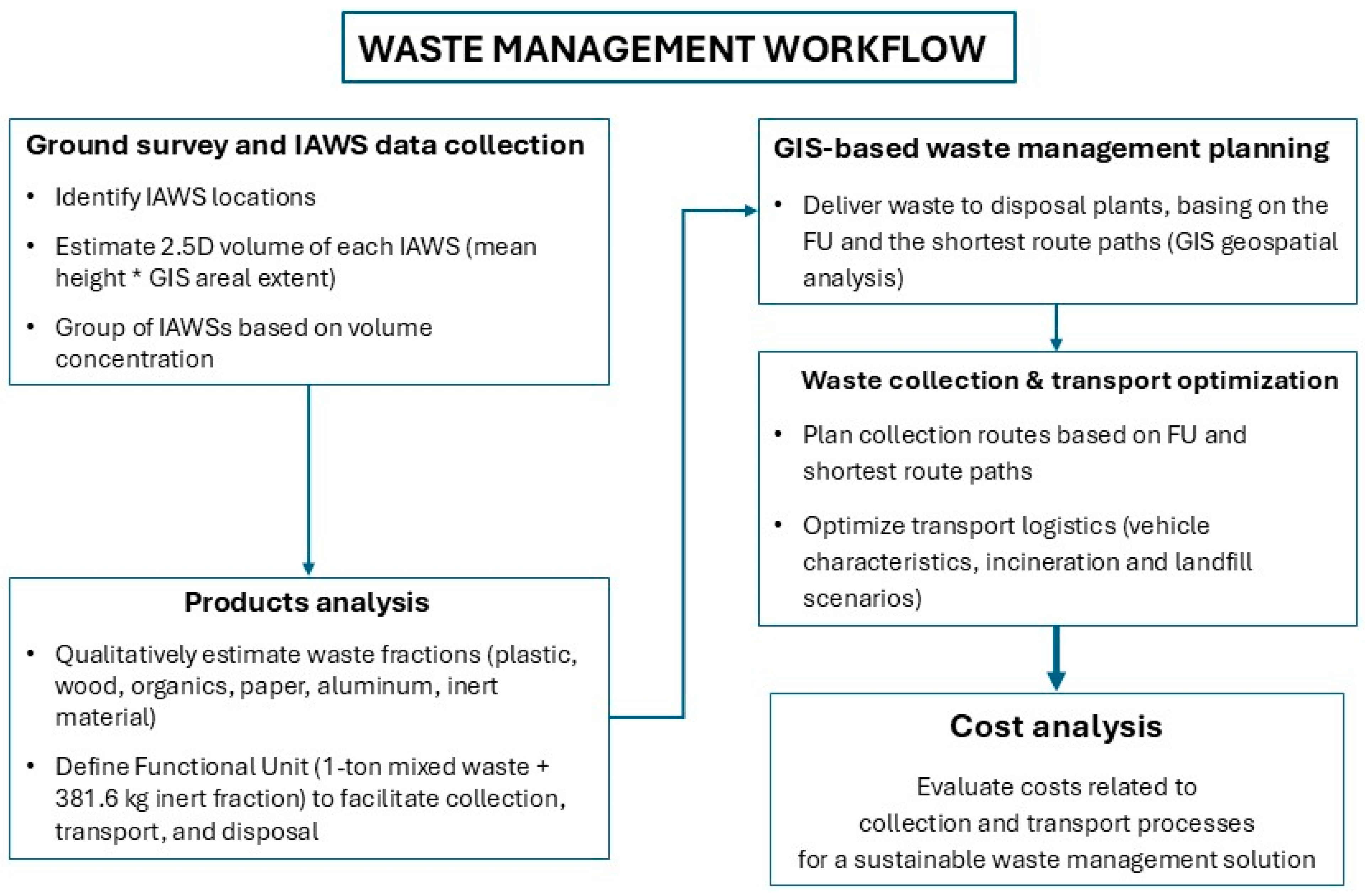
2. Materials and Methods

Initially, this study concerns the elaboration of ancillary information as geospatial data, generating analysis and thematic maps within the study area. From a baseline survey, reference is made to all those layers that, included into a GIS framework, may be useful to understand the territory (e.g., sample multipoint, road network polylines, administrative polygons). The study focuses on six municipalities within the province of Catanzaro (Calabria, Italy), aiming to manage Illegal Abandoned Waste Sites (IAWSs) through an integrated GIS-based approach. IAWSs, identified through both remote and ground sensing activities, serve as the primary source of data for obtaining results essential to the final cost analysis. IAWSs represent the main data layer of this study, incorporating geographical information (e.g., localization), product analysis, and spatial data such as point and volume density maps. In detail, IAWSs are identified both from remote and ground sensing activities, converted into spatial data, and subsequently elaborated and managed to support the cost analysis assessment. Accordingly, spatial data modeling is applied by including 2.5D volume analysis, product analysis, shortest paths algorithms, and programming languages.

This methodology aims to obtain minimal-cost routes between sources and destinations. Hence, in GIS software, Dijkstra’s algorithm is used to perform cost analysis by incorporating data related to the transport of waste to the nearest municipal collector and/or disposal plant. Thus, as illustrated in Figure 1, a cost analysis is finally defined, employing geospatial data such as the road network, territory information, vehicle speed, and topological tolerances.

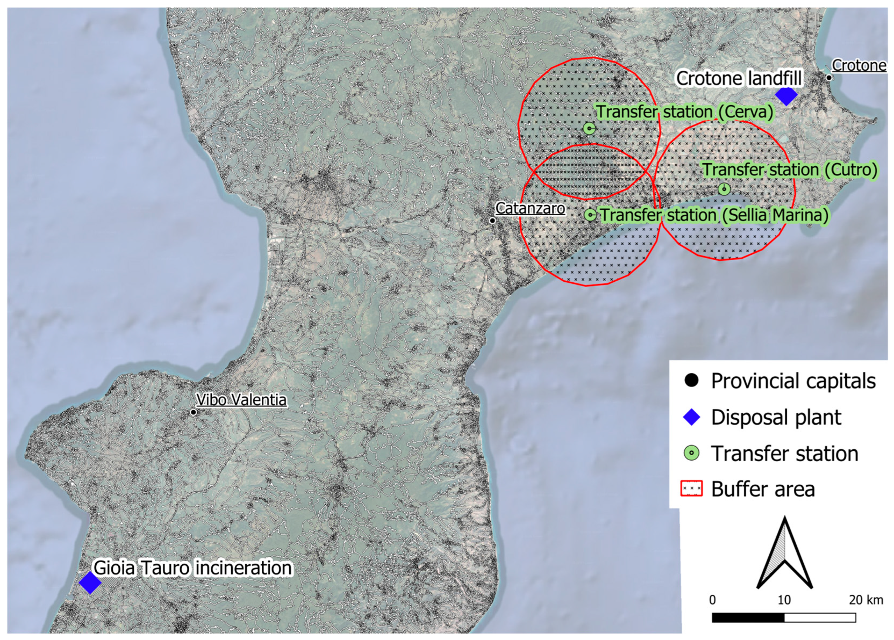
2.1. Overview and Ancillary Data

In recent years, a slight expansion in waste services has been observed in Calabria. From 2015 to 2021 there was an increase in specialized waste treatment facilities, with composting plants growing by 4 units and landfills decreasing by 1 unit (

Table 1. Waste treatment facilities in the Calabria region during the years 2015 and 2021 [23].

Facilities	Units 2015	Units 2021
Composting	7	11
Aerobic and anaerobic integrated system	0	1
Anaerobic digestion	0	0
Mechanical biological treatment	8	8
Incineration	1	1
Co-incineration	1	1
Landfill	6	5

).

The analysis of waste collection in the municipalities under study for the year 2021 provides key insights into the efficiency and distribution of different waste fractions. The available data reveal a significant disparity in the collection of specific waste types, with notable gaps in metal and wood collection, particularly for the municipalities of Sersale and Soveria Simeri, where data are not reported. Similarly, the collection of plastic waste appears to be extremely limited, especially in Cropani and Sersale. The absence of bulky waste collection data for Sersale further highlights inconsistencies in waste management practices across the study area. Conversely, the collection of organic waste, paper, glass, and unsorted fractions is substantial, reflecting a structured approach to managing these types of waste [23]. However, the high values associated with the unsorted fraction indicate potential inefficiencies in the collection and recycling processes. This suggests a considerable opportunity for improvement, particularly in enhancing the collection of metal and plastic waste to reduce the volume of unsorted materials. To better understand the spatial distribution and patterns of waste collection, ancillary data have been incorporated into the analysis. These supplementary datasets provide essential context, helping to elucidate the relationships between waste collection efficiency and geographical factors. Moreover, the ancillary data include information on road networks, district boundaries, and transfer stations, which are fundamental to GIS-based analysis. These spatial datasets, downloaded from the national geoportal service of the Italian Ministry of Environment and Energy Security in October 2023, are formatted as geospatial data and adhere to the standards outlined in Directive 2007/2/EC. The datasets consist of simple geometric elements, points, lines, and polygons, encoded and stored according to their respective coordinates. Each spatial element is associated with an attribute record, allowing for an integrated analysis of waste collection efficiency within the geographical framework of the study area. The role of these spatial datasets is crucial for identifying patterns and inefficiencies in waste collection services. The road network, for example, influences the accessibility of collection points and transfer stations, which in turn affects the frequency and efficiency of waste collection. District boundaries help to delineate administrative responsibilities and highlight regional disparities in waste management performance. Similarly, transfer station locations provide insights into logistical challenges that may impact collection efficiency and overall waste processing. Accordingly, the integration of GIS-based analysis with waste collection data offers a powerful tool for local authorities to optimize collection routes, identify underserved areas, and implement strategic improvements.

According to the INTESA project, the municipality waste collection data are reported in Figure 2. Data pertains to the year 2021 show that information regarding the collection of metals and wood are notably scarce. Particularly, for Sersale and Soveria Simeri, metals and wood information are not reported. Additionally, the collection of the plastic fraction appears to be very limited, especially in Cropani and Sersale. Moreover, about Sersale, bulky collection data are absent.

The road network dataset includes all major and minor roads within the study area, taking into account connectivity, accessibility, and potential influences on spatial phenomena. District boundaries include information regarding the municipalities of Sersale, Cropani, and Soveria Simeri. Moreover, three transfer stations are considered, referring to the municipalities of Cerva, Cutro, and Sellia Marina. Regarding the waste treatment facilities, the Gioia Tauro incineration plant and the Crotone landfill are included in the dataset as key elements for understanding waste management in the region.

The spatial distribution of the waste disposal sites (three transfer stations and two waste plants) is also represented in Figure 3. These facilities are crucial for the spatial analysis of waste disposal infrastructure, enabling the assessment of environmental and logistical impacts within the Circular Economy context. Thus, the integration of waste data with geospatial information can provide a more comprehensive view of the territorial dynamics and the relationships between different infrastructure elements, facilitating the optimization of waste management services.

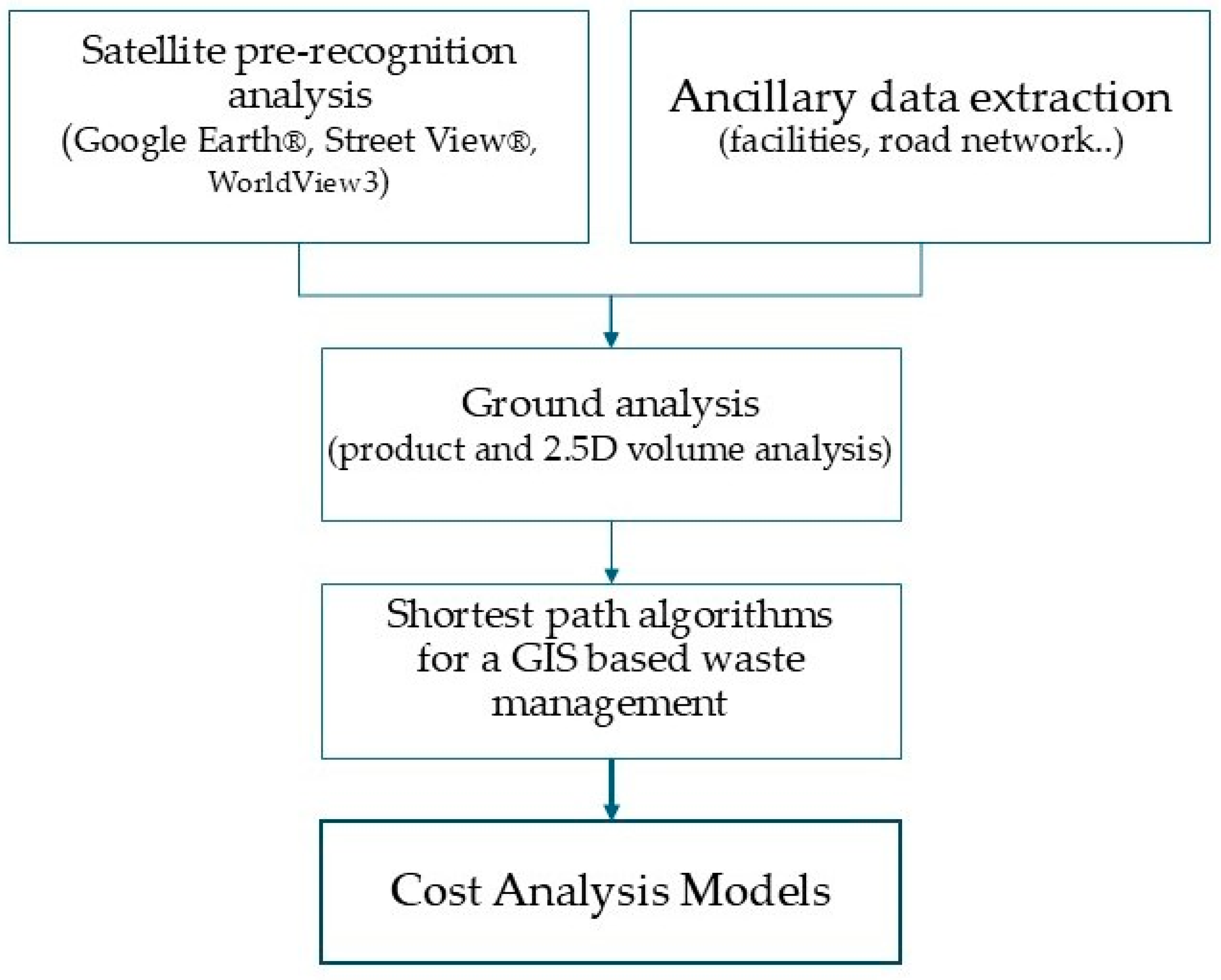
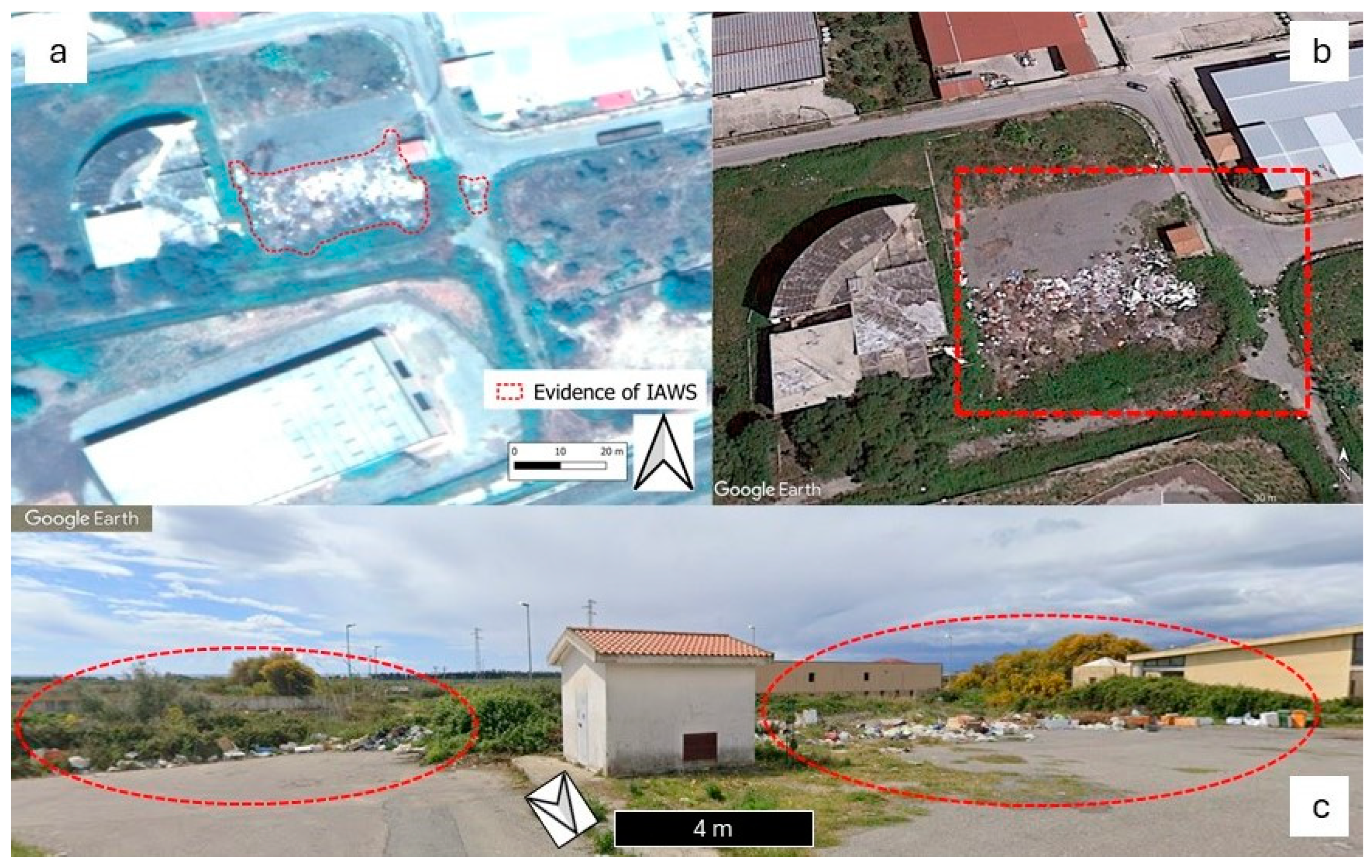
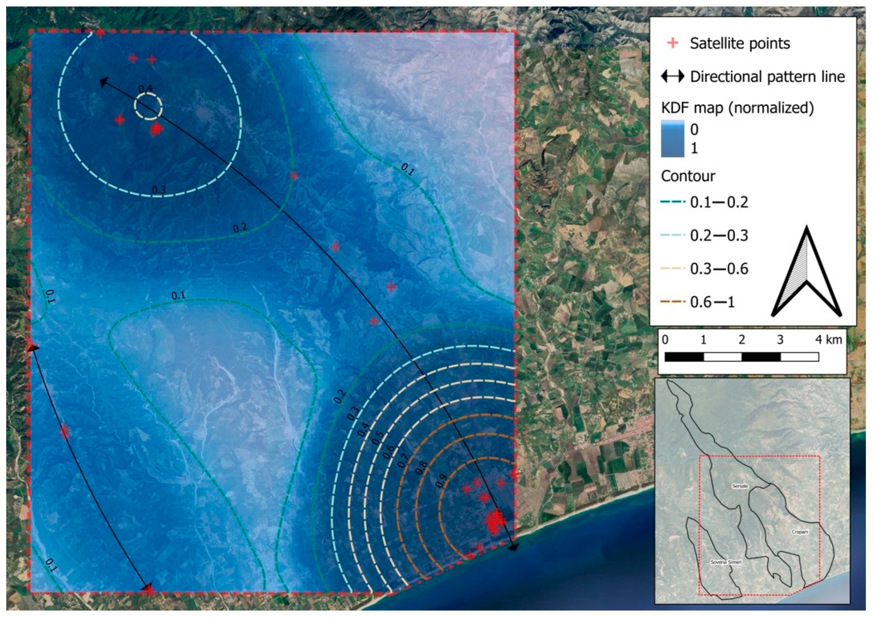
2.2. Satellite Pre-Recognition Phase

The use of Google Earth^® and Street View^® has been persistent over the past decade, showing a significant contribution to remote sensing and GIS technologies [24,25]. Accordingly, a preliminary analysis spanning 2021 to 2023 occurred, combining Google Earth^®, Street View^®, and high-resolution WorldView-3 imagery. The examination occurred through a photo-interpretative analysis of critical areas across large portions of the territory potentially characterized by the presence of IAWSs. Indeed, the accessibility of these platforms allows community involvement, enhancing the overall effectiveness of waste management efforts. On the other hand, as far as satellite sensors are concerned, efforts are made to converge toward the use of localized Very High Resolution (VHR) image acquisition, providing high spatial resolution (30/50 cm in panchromatic) through focused data processing. The WorldView-3 image processing used for this purpose employs the Intensity Hue Saturation (IHS) pansharpening technique, which enhances image resolution by transforming RGB components into the IHS color system, replacing the intensity band with panchromatic images [26]. According to the photointerpretative analysis, a specific workflow to determine potential IAWSs is obtained, concerning the recognition of sites in nadiral position (Google Earth^® and WorldView-3) and through street-level images (Google Street View^®).

Kernel Density Function (KDF) Maps and Python Script Design

As in the previous analysis, KDF maps are obtained to highlight critical areas, considering retrieved spatial point data and calculating a smoothly curved surface over each feature recognized by remote and/or ground sensing activities. As shown in Equation (1), the predicted density at unknown locations is determined by the following formula, involving radius distances and eventual field values of points within the specified radius:

$$\mathrm{P}={\displaystyle \frac{1}{{\left(radius\right)}^2}}\sum _{i=1}^n\left[{\displaystyle \frac{3}{\pi }}·{pop}_i{\left(1-{\left({\displaystyle \frac{{dist}_i}{radius}}\right)}^2\right)}^2\right],{dist}_i<radius$$

(1)

where i represents the i-input point ranging from 1 to n; the summation includes only points falling within the specified radius distance of the (x, y) location; pop_i denotes the population field value of each point i; radius is the radial distance from the (x, y) point; and dist_i stands for the distance between point i and the (x, y) location.

Consequently, a Python script was developed to process geospatial data contained in a shapefile, specifically a point layer, by performing polynomial interpolation to create a curve that best fits the potential IAWS points. Thus, an interpolated curve is generated as a new line feature in a separate shapefile. The script utilizes the import of necessary libraries as GeoPandas, NumPy, and Shapely, which are used respectively for handling geospatial data, performing numerical computations (e.g., polynomial fitting), and manipulating geometric objects (e.g., lines). Moreover, the script defines the following function: interpolate polynomial from shapefile, which takes the following three parameters: (1) the path to the input shapefile containing point data; (2) the degree of the polynomial to be fitted; and (3) the path to the output shapefile where the interpolated line is saved. Inside the function, the input shapefile is read into a dataframe using GeoPandas, allowing for easy manipulation of geometric data and associated attributes. To facilitate numerical operations required for interpolation, the script extracts the coordinates of each point in the shapefile, storing them as a list of tuples, and converting this to a NumPy array. A polynomial is fitted to the data using numpy.polyfit, which computes the coefficients of a polynomial of the specified degree that best fits the data in a least-squares sense. This polynomial is represented as a function, allowing the calculation of new y-values for a range of x-values. Hence, by using the polynomial function, a smooth curve that fits the input points is obtained, combined into a set of coordinates that describe the interpolated line. A LineString object is created from these coordinates using Shapely, representing the interpolated curve as a geometric line feature. This line is then placed into a new dataframe, preserving the original coordinate reference system of the input data to ensure geospatial consistency. The script writes the dataframe containing the interpolated line into a new output shapefile, ready to be used for further geospatial analysis in GIS software to understand patterns and support informed decision-making.

2.3. Ground Investigation (2.5D Volumes and Product Analysis)

Based on satellite monitoring activities spanning 2021 to 2023, a piloted ground survey was performed in November 2023 to identify IAWSs within the study area. Ground data collection was conducted in the municipalities of Soveria Simeri, Sersale, and Cropani, and expanded to the nearby districts covering the coastal areas and including Sellia Marina, Belcastro, and Botricello municipalities. In the context of environmental monitoring and illegal waste management, the identification and quantification of IAWSs is fundamental. Accordingly, from the field survey, ground images and Global Positioning System (GPS) data were collected to create a comprehensive ground dataset. These data form the basis for a geospatial analysis aimed to identify and map IAWSs across the territory. To extend the spatial analysis of IAWSs beyond two dimensions, ground-based images and on-site evaluations are used to approximate the height and area of waste piles present at each site. The process begins with the acquisition of detailed images from various angles at each IAWS, followed by the digitization of these images to facilitate the extraction of spatial information. The integration of ground-based and satellite-based imagery enables the approximation of average waste pile height and area, allowing for the calculation of the volume at each site. Thus, the average waste pile height derived from the field image analysis is combined with the retrieval of areal extent of each IAWS. The volume (V) of waste piles at each site is computed by using the following basic geometric approximation (rectangular cuboid):

$$\mathrm{V}=Ab\times h$$

where the area is approximated to a rectangle occupied by the waste site (as obtained from geospatial analysis). Ab is related to the base surface area and h to the approximate height of the waste pile (Figure 4), as estimated from the field and ground-based imagery.

These volumetric data provide a 2.5-dimensional perspective on the extent of waste accumulation, offering a more comprehensive understanding of the scale of illegal dumping activities across the study area.

Consequently, a systematic field investigation and product analysis of the waste present at each IAWS was conducted. This step involved field activities and ground-based image photointerpretation (visual analysis), aiming to detect and classify the different types of materials within the waste piles.

For each of the 171 identified sampling sites, multiple images were acquired to enable a detailed visual analysis of the waste piles. This process facilitates the detection and categorization of various material types within the areas of interest. As a result, the classification of materials within the waste piles is inherently subject to an estimation error, due to the potential uncertainties in visual assessments, variations in waste material, and the influence of perspective on image interpretation. Accordingly, the ground survey identified a variety of materials across the study area, including bulky items (e.g., washing machines, refrigerators, ovens, TVs, water heaters, furniture, buckets, chairs, mattresses, sofas), paperboard, garbage bags with clear packaging, garbage bags with no clear packaging, construction and demolition waste (e.g., excavated soil, bathroom fixtures, pipes, insulation sheathing, metal sheets, garden trimmings, burned remains). Therefore, aiming to simplify the procedure of classification, only the following materials are considered: steel, aluminum, plastic, wood, textile, glass, inert material, paper, and organic fraction. In parallel, a qualitative product analysis of the waste at each IAWS is conducted, using both on-site activities and ground-level photointerpretation.

Figure 5 shows an example of a sampling site where product and 2.5D volume analyses were conducted in a homogeneous waste material context (primarily C&D waste). For the remaining sampling sites, this approach allows for a qualitative classification of waste materials, identifying waste product such as bulky items, paperboard, plastics, aluminum, glass, wood, different types of garbage bags, and construction-related waste. Again, it is important to note that visual qualitative assessments are subject to estimation error due to potential uncertainties related to disturbance during the on-site survey or image quality, effects of lighting and perspective, variable materials, and the presence of voids or empty spaces. Accordingly, during on-site inspections at all 171 points, we collected more than 400 images, allowing experts to recognize the material collected at abandoned waste sites. Selected examples are reported in the GitHub repository (https://github.com/AlfRag91/IAWSs.git, accessed on 29 January 2025).

The data presented in

Table 2. Estimated values for each waste fraction, considering only the following materials: steel, aluminum, plastic, wood, textile, glass, inert material, paper, and organic fraction. References to ISPRA, Municipal Waste Report—2022 [23]; WEEE Coordination Center [27]; and Agbogbloshie Makerspace Platform [28]); Guidance on the classification and assessment of waste (1st Edition v1.2.GB) Technical Guidance WM3 (https://github.com/AlfRag91/IAWSs.git); http://zerowastecities.eu [29]; http://www-pub.iaea.org [30].

Class	Item	Material	Percentage	Density (kg/m3)	Mean Mass (kg)	Reference
Bulk	Washing machine	Steel	37%		40	https://www.cdcraee.it/, accessed on 29 January 2025 [27]
		Al and Cu	2%
		Plastic	13%
	Fridge	Steel	47%		50	https://www.cdcraee.it/, accessed on 29 January 2025 [27]
		Aluminum	5%
		Plastic	11%
	Oven	Steel	49%		15	https://qamp.net/library/microwave-ovens/, accessed on 29 January 2025 [28]
		Al and Cu	12%
		Plastic	1%
	TV (CRT)	Steel	14%		12	https://www.cdcraee.it/, accessed on 29 January 2025 [29,30]
		Al and Cu	5%
		Plastic	20%
		Glass	48%
	Water heater	Steel	91%		12	https://www.cdcraee.it/, accessed on 29 January 2025 [29,30]
		Al and Cu	2%
		Plastic	5%
	Furniture_w	Wood	100%	550		[23]
	Furniture_p	Plastic	100%	1400
	Furniture_s	Steel	100%	7500
	Bucket	Plastic	100%	1400		[23]
	Mattress	Textile	100%		20	[23]
	Sofa	Wood	20%		50	[23]
		Textile	80%
Paperboard		Paper	100%	1000
Garbage bag without clear packaging		Plastic	10%	900		[23]
		Glass	31%	2600
		Al and Cu	1%	2700
		Steel	2%	7500
		Paper	54%	1000
		Wood	2%	550
C&D	Excavated soil	Inert	100%	1700		[23]
	Bathroom fixture	Inert	100%	2300
	Pipes	Plastic	100%	1400
	Insulation sheathing	Plastic	100%	1400
	Metal sheet	Plastic	100%	1500
		Steel	100%	7850
	Garden waste	Organic fraction	100%	400

are sourced from the ISPRA Municipal Waste Report—2022 [23], the WEEE Coordination Center [27], Agbogbloshie Makerspace Platform [28], and others [29,30]. These sources provide guidelines and reference values for waste characterization, which were used to estimate the weight and volume of each waste fraction. To enhance clarity, the data sources are also indicated in the title of Table 2. The methodology follows standard procedures outlined in the report, ensuring consistency and reliability in the conversion of volumetric percentages into mass percentages. To this purpose, the following equations are used for calculating weight, density, and total percentage for each material (plastic, glass, aluminum, steel, etc.):

$$Weight=Density\times VolumePercentage$$

$$MaterialPercentage={\displaystyle \frac{\Sigma WeightofMaterial}{totalWeight}}\times 100$$

Accordingly, given the complexity related to product characterization, only the following classes of material are considered: (a) Plastic; (b) Glass; (c) Steel; (d) Aluminum; (e) Wood; (f) Paper; (g) Textile; (h) Inert material; and (i) Organic fraction. As previously mentioned, these material fractions are presented as volumetric percentages which have been converted into mass percentages by considering the average weight of bulky waste, the density of each material fraction, and the volume calculated (Table 2). For bulky waste, an average material composition is considered. For instance, a washing machine consists of the following percentages: 37% steel, 2% aluminum, and 13% plastic [27]. The same method is applied to other items such as refrigerators, ovens, TVs, water heaters, mattresses, and sofas (for references, see Table 2; for data sources and computations, see https://github.com/AlfRag91/IAWSs.git). In the case of garbage bags without clear packaging, the internal material composition is estimated through a rough visual assessment as applied by ISPRA (2022) [23]. To ensure consistency, ISPRA’s Municipal Waste Report (2022) [23], the WEEE Coordination Center, CdC RAEE [27], and the Agbogbloshie Makerspace Platform [28], references provide benchmark values and guidelines for waste characterization, which are essential for converting volumetric data.

The integrated methodology, combining geospatial analysis (via QGIS and Dijkstra’s algorithm for route optimization) with expert photointerpretation and Excel-based scenario analysis, provides a comprehensive framework for assessing IAWSs.

To manage all these types of data, a structured Excel-based scenario analysis tool is provided, useful to process and analyze waste composition data efficiently (https://github.com/AlfRag91/IAWSs.git). The tool leverages the background data described in the previous sections and provides a structured approach to evaluating various waste management scenarios. By incorporating key parameters such as material density, weight distribution, and volume contributions, the tool allows users to assess the impact of different waste disposal strategies. The Excel-based model is designed to be user-friendly, enabling stakeholders to input new data, adjust key variables, and visualize results through automated calculations.

2.4. Application of Dijkstra’s Algorithm in a GIS Environment for Waste Transport Planning

Dijkstra’s algorithm is a fundamental method in graph theory for finding the shortest path between nodes in a network. Dijkstra’s algorithm starts by selecting a source node and iteratively explores all connected nodes, determining the minimum cumulative distance to reach each node from the source. This process involves maintaining two tables: a permanent table, which records the shortest known distance to each node, and a temporary table, which holds nodes that have yet to be fully processed. As the algorithm increases, nodes with the shortest distances in the temporary table are moved to the permanent table until all nodes are processed, yielding the shortest path from the source to all other nodes in the network [19]. Within the GIS environment, Dijkstra’s algorithms are particularly useful for waste collection planning optimization, ensuring the operational efficiency of waste management systems [16,17,18,19,20,21,22]. This methodology allows us to identify the shortest paths between IAWSs and designated transfer stations, minimizing travel time and fuel consumption in a Circular Economy context. Accordingly, to perform the calculation of distances between each point and a transfer station associated, routes are calculated individually based on the Calabrian road network. Settings are adjusted to influence the route calculation by specifying attributes of the vector data (e.g., vehicle speed, topological tolerances, choice of certain roads) and adjusting the parameters of the search algorithm, aiming to obtain results best suited to the operator’s needs. Accordingly, speed field values correspond to 50 km/h for the edges of the network, while the topological tolerance values correspond to 10 m. From what the present work concerns, by using the software QuantumGIS (version 3.42.1 ‘Münster’), it is possible to use a tool based on Dijkstra’s algorithm to optimize the waste collection routes within the study area. Thus, QGIS’s “Shortest Path (point to layer)” tool is used to calculate the shortest path between a starting point and a destination. Three transfer stations, selected for the algorithm, are responsible for managing waste within a 10 km radius. This spatial division ensures that waste collection is distributed throughout the entire study area, where each transfer station manages the waste from sites occurring within its designated area. In the end, for each transfer station, two final disposal plants are assigned (Crotone landfill and Gioia Tauro incineration), depending on the type of material to be disposed of.

2.5. Cost Analysis (Functional Unit, Transport, and Plant Management)

In this section, the application of Bizagi Modeler open-source software is outlined as a tool for developing waste management within a cost analysis context. Bizagi Modeler enhances the capabilities of processes by offering a cloud-based system, allowing us to manage and share information. Hence, Bizagi Modeler is chosen for its ability to model complex waste management processes, enabling the creation of a detailed procedure that visualizes every step in the waste management workflow. Each process is modeled using a series of “pools”, representing activities involved in waste management planning. Pools are flexible and allow for easy connectivity between different steps in the process, handling data for an accurate waste management analysis. Bizagi Modeler is also used to optimize waste management planning by simulating different scenarios, such as changes to collection routes or to the waste disposal plant. By visualizing these scenarios within the process model, decision-makers can assess the potential impact of each change on both the environment and costs. The two scenarios are defined as follows: (Scenario 1) Removal of the illegally dumped waste and its disposal in the landfill (Crotone plant); (Scenario 2) Removal of the illegally dumped waste and its incineration (Gioia Tauro plant).

For this study, a Functional Unit (FU) is defined as 1 ton of mixed waste, allowing for a comprehensive understanding of how 1 ton can interact with the environment based on the cost analysis process [22]. In detail, FU is a fundamental concept that ensures consistency and clarity in evaluating the environmental impacts of a product or process, becoming a reference for all calculations in different cost analysis assessments. In detail, to determine the FU, 33 sites concerning more than 90% of inhert material were excluded, simplifing the cost analysis for this study. Additionally, the inert fraction, excluded from the mixed waste category, is normalized relative to the FU. Hence, defining the FU properly is important to compare different cost analysis processes conducted in comparable contexts [31].

Essentially, following the pre-analysis phase using remote sensing technologies (see Section 2.2), the waste management process begins with a ground survey, identifying IAWS locations. Subsequently, 2.5D volume estimations are conducted by considering both the area and mean waste pile height of each sampling site. This information is essential for grouping IAWSs based on volume concentration, optimizing collection and transport strategies (see Section 2.3). Consequently, a qualitative product analysis of waste fractions, including plastic, wood, organics, paper, aluminum, and inert materials, is undertaken. This leads to the definition of a Functional Unit (FU) of 1 ton of mixed waste plus 381.6 kg of inert material, which standardizes waste measurement and simplifies transport and disposal planning. Moreover, the FU also provides a structured reference for cost analysis, preparing for an efficient waste transport strategic route plan based on IAWS volume groups (see Section 2.3). Transport costs depend on distances and vehicle type, basing the strategy on the FU and the shortest route paths by using a GIS-based geospatial analysis (

Table 3. Transport and plant management specific costs for the main points [23]. In the transport and plant management section, related costs are provided by following the Ministry of Infrastructure and Transport data (2022) [32], ISPRA (2022) [23], and Calabria Region Price Analysis—Civil Works (2022) (see the PDF document at https://github.com/AlfRag91/IAWSs.git).

Category	Costs
Transport	Point 1	Cost of transport up to 10 km	9.77 €/m3
		Cost of transport for each 5 km over first 10 km	4.62 €/m3
	Point 2	Mean cost of transport for a vehicle of category D (more than 26 tons)	1.6 €/km
Plant management	Point 3	Mean cost of landfill waste management	100 €/t
		Mean cost of incineration waste management	110 €/t

). Accordingly, the framework is based on references such as the Ministry of Infrastructure and Transport (2022), ISPRA (2022) [23], Calabria Region Price Analysis—Civil Works (2022), and Ministry of Infrastructure and Transport data (2022) [32]. For the previous and more references related to transport and vehicle costs, refer to the GitHub repository “https://github.com/AlfRag91/IAWSs.git”.

The cost analysis focuses on key steps involved in the transport of waste and the selection of the disposal site, organized into the following two categories:

(1)

Transport and waste management category. The transportation costs, firstly, concern the paths from IAWSs to transfer stations and, secondly, the paths from transfer stations to disposal plants. The cost of transport in Italy is influenced by various factors, including vehicle acquisition, fuel prices, maintenance, and personnel expenses. Accordingly, the Italian Ministry of Infrastructure and Transport periodically publishes indicative cost values for the road transport sector. Following the provisions of Article 1, paragraph 250, of Law No. 190 of 23 December 2014, these reference values replaced the previously mandated “minimum transport costs” established under Article 83-bis of Decree-Law No. 112 of 25 June 2008. The latest update, based on inflation trends recorded by ISTAT and fuel price variations reported by the Ministry of Ecological Transition, provides revised unit costs per kilometer as of January 2022 [33].

(2)

Waste treatment plant category. The waste treatment plant categories are considered both for the landfill and incineration scenarios. Direct sources for costs are associated in relation to the category of management plant.

The collected waste is then delivered to disposal plants, considering transport and plant management specific costs. In the end, the approach focuses on cost-effectiveness rather than a traditional cost–benefit analysis, aiming to develop an optimized workflow that minimizes costs while maintaining efficiency (Figure 6). Moreover, to ensure reliability, the cost analysis assumptions for the Functional Unit (FU: 1 ton + 381.6 kg of inert material) refer to the Ecoinvent database [34]. All assumptions and references used in this analysis are also available in the GitHub repository: https://github.com/AlfRag91/IAWSs.git.

3. Results

In the first stage of this study, basic spatial information was acquired from existing maps and cartographies of the territory. Reference was made to the road network data, cartographies, and to all those layers that may be useful to understand the territory. All data were incorporated into a GIS-based framework, together with information collected about IAWSs identified from satellite and ground activities. An additional aspect of this study concerns the collection of information about the relevant legislation in terms of waste management, delivering cost analysis from the data acquired within the study area. Hence, data resulting from project activities are georeferenced and processed within a GIS-based framework, building a database concerning some fundamental information derived from baseline, remote, and ground survey activities. Accordingly, a cost analysis is provided for two scenarios: (Scenario 1) Removal of the illegally dumped waste and its disposal in the landfill (Crotone plant); (Scenario 2) Removal of the illegally dumped waste and its incineration (Gioia Tauro plant).

3.1. Satellite Pre-Recognition Analysis

The thematic map resulting from the satellite pre-recognition phase highlights two main areas with a significant presence of potential IAWSs. These areas were identified using a comprehensive methodology that combines satellite imagery, such as Google Earth^® and WorldView-3, with a further street-level verification through Google Street View^®. By using the Google Earth Pro^® platform, the search for litter evidence over the municipalities within the Catanzaro province allows the identification and analysis of satellite images from different time periods. Each site is represented by its coordinates, a number, and a symbol. If the street-level verification through Google Street View is not possible, three WorldView-3 pansharpened images are used to compare Google Earth Pro evidence. Hence, the integration of these data sources can provide a multitemporal and multidimensional perspective on the distribution of IAWSs within the municipalities. According to this, potential IAWSs are identified by integrating evidence from the aforementioned data sources over the period from 2021 to 2023.

An example is shown in the following image (Figure 7), which includes data from Google Earth, Google Street View, and a WorldView-3 pansharpened image. The research conducted through Street View confirms the occurrence of IAWSs evidence, revealing the presence of different waste types abandoned in the surroundings (urban and inhabited). It should be noted that many sites are characterized by the presence of abandoned material, such as paper, plastic, glass debris, organic waste, and garbage bags that are not properly closed. Also notable is the presence of household appliances, abandoned mattresses, and building materials. From a regional point of view, and following Equation (1), a Kernel Density Function (KDF) map is obtained, starting from the satellite pre-recognition of potential IAWS points. As outlined in Section 3.2, from the 40 points detected by using remote sensing, 25 points are verified using a 300 m buffer during a ground-truth survey (for this purpose, a Python script was developed).

As shown in Figure 8, a total of 40 potential IAWS points were identified, allowing the elaboration of the KDF map and showing a kernel surface fitted over the study area. The contribution of the points to the density is equal to the value of the kernel surface at the raster cell center. The use of KDF estimation for the previous map creates a smoothly curved surface over each point, allowing the visualization of critical areas with a higher density of IAWSs. The density calculation considers the population field value within a specified radius, offering insights for the spatial patterns and potential drivers about waste site locations. This approach highlights hotspots where waste management efforts might need to be prioritized, emphasizing areas with higher environmental and public health impacts. In the equation used to calculate the kernel function, only the points falling within the specified radius are included, denoting population density values. The theme indicating values for each feature is related to the “id” population field, where each point counts once. The search radius (bandwidth) for calculating density is 8000 m (using planar distances, since the data are stored in a metric coordinate system) and the output raster cell size corresponds to 100 m. As detected from remote sensing techniques, it can be noticed that the southeastern part of the study area is characterized by more potential IAWS presence. Additionally, the polynomial interpolation method, applied through Python scripts, allows the creation of smooth curves that fit the IAWS points across the study area. This interpolated line provides a visual representation of the pattern formed by these sites, aiding in understanding the spatial dynamics at play. Thus, the KDF map reveals two distinct regions where potential IAWSs are concentrated. The larger of the two areas is located to the east and is characterized by a notable density of the sites. Both areas are represented by lines oriented from northwest to southeast, indicating a directional pattern in the distribution of waste sites. These orientations could suggest the influence of certain geographical or human factors in IAWS distribution, such as transportation routes, which may facilitate the abandonment and accumulation of waste.

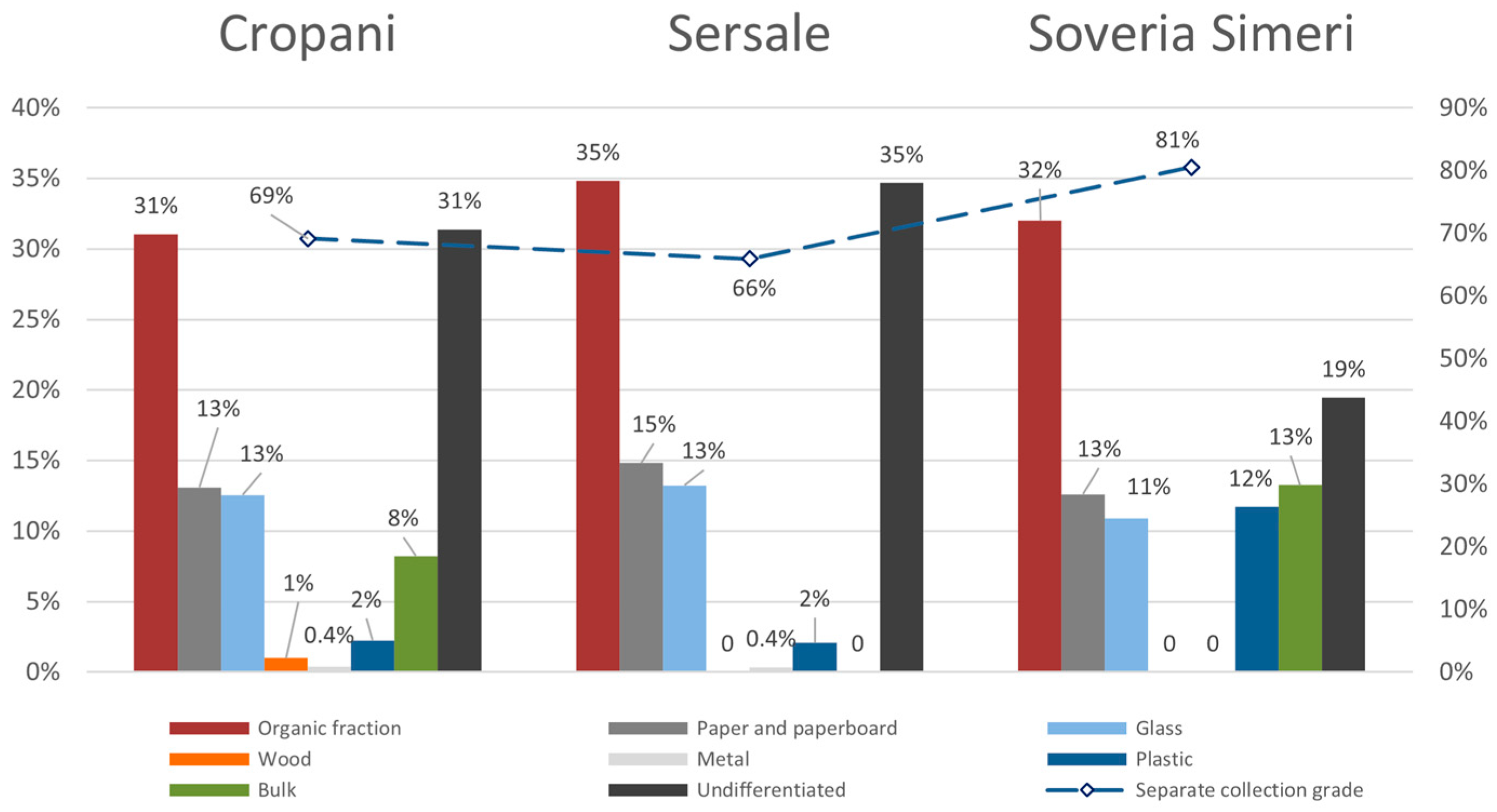
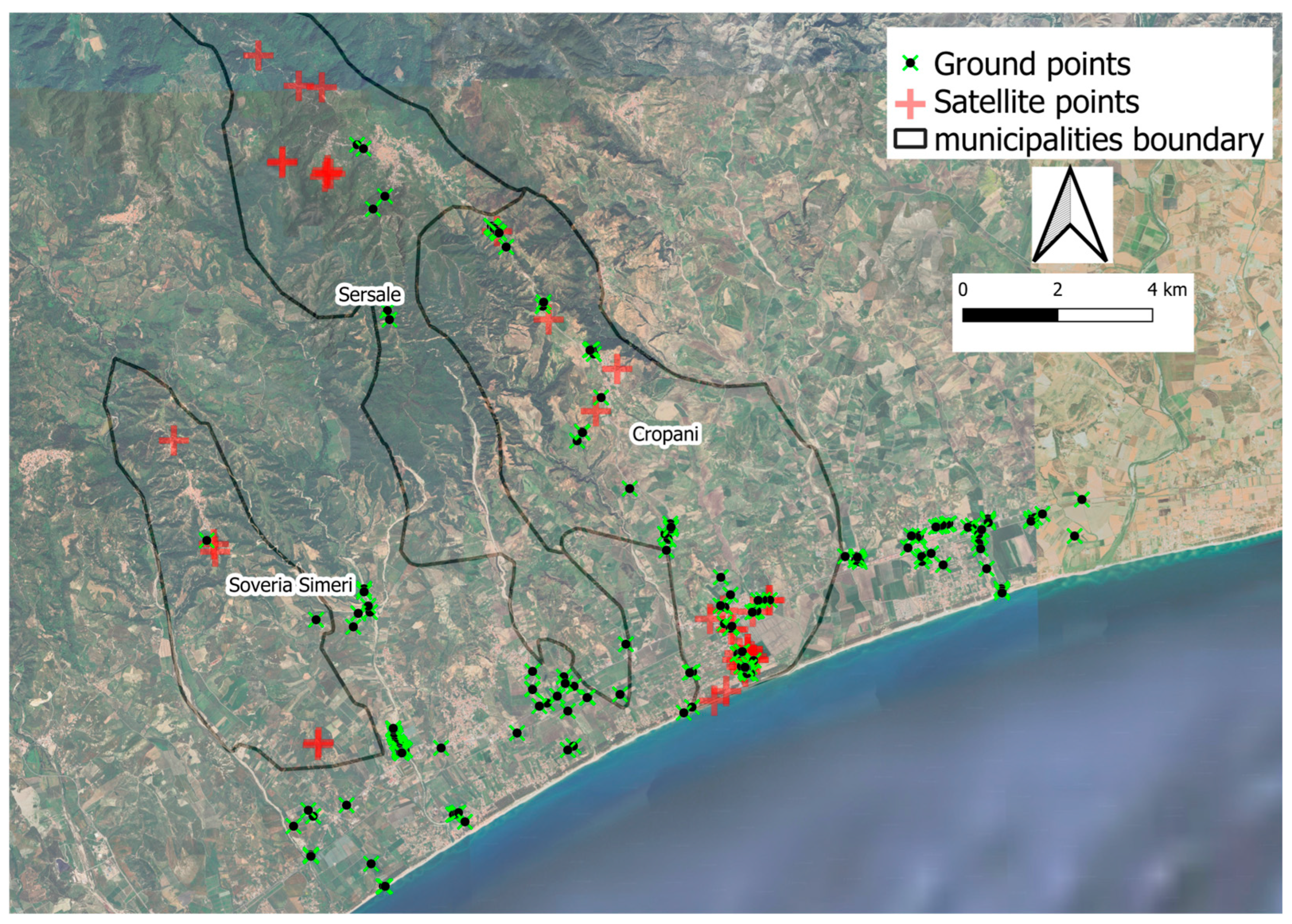
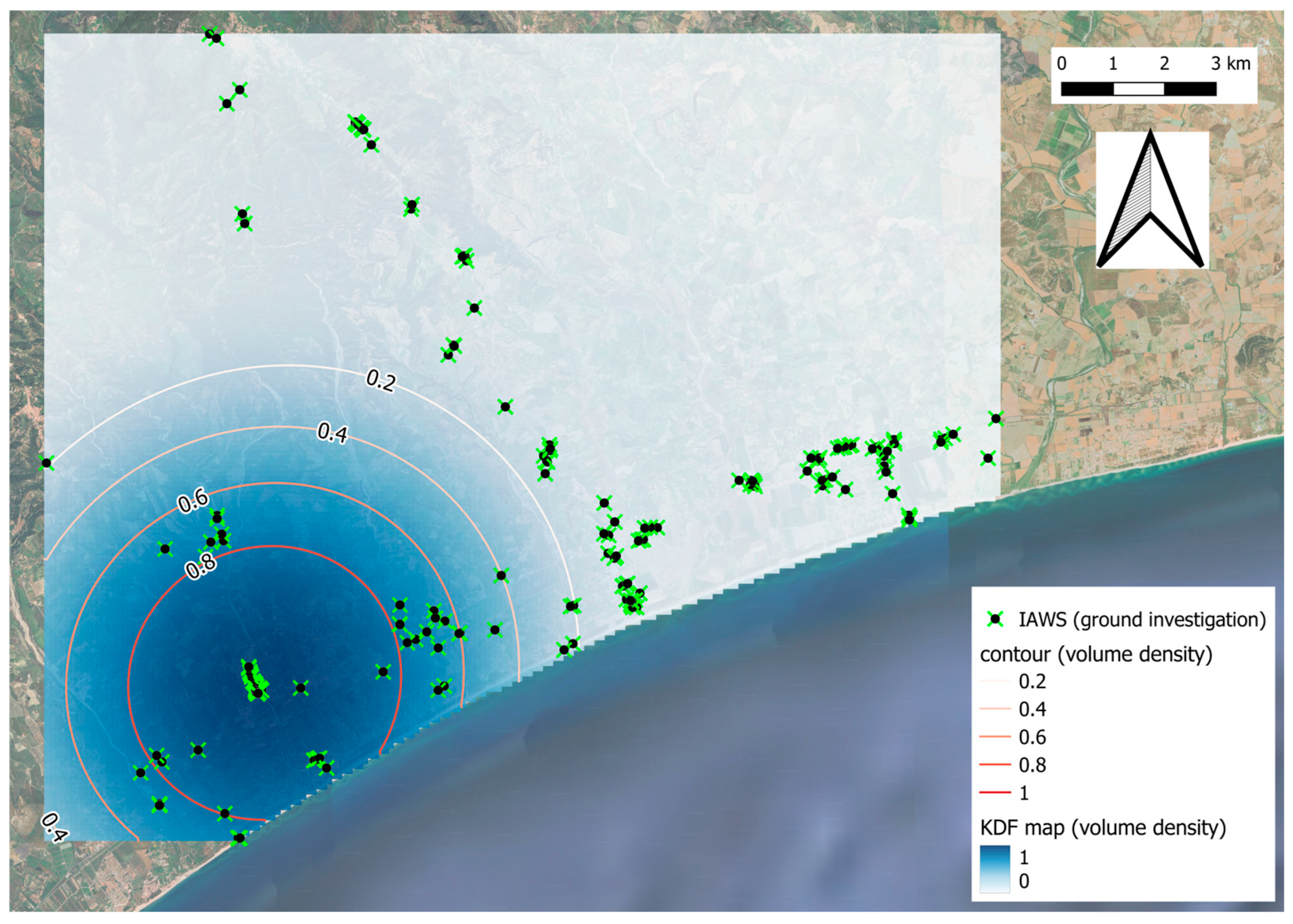
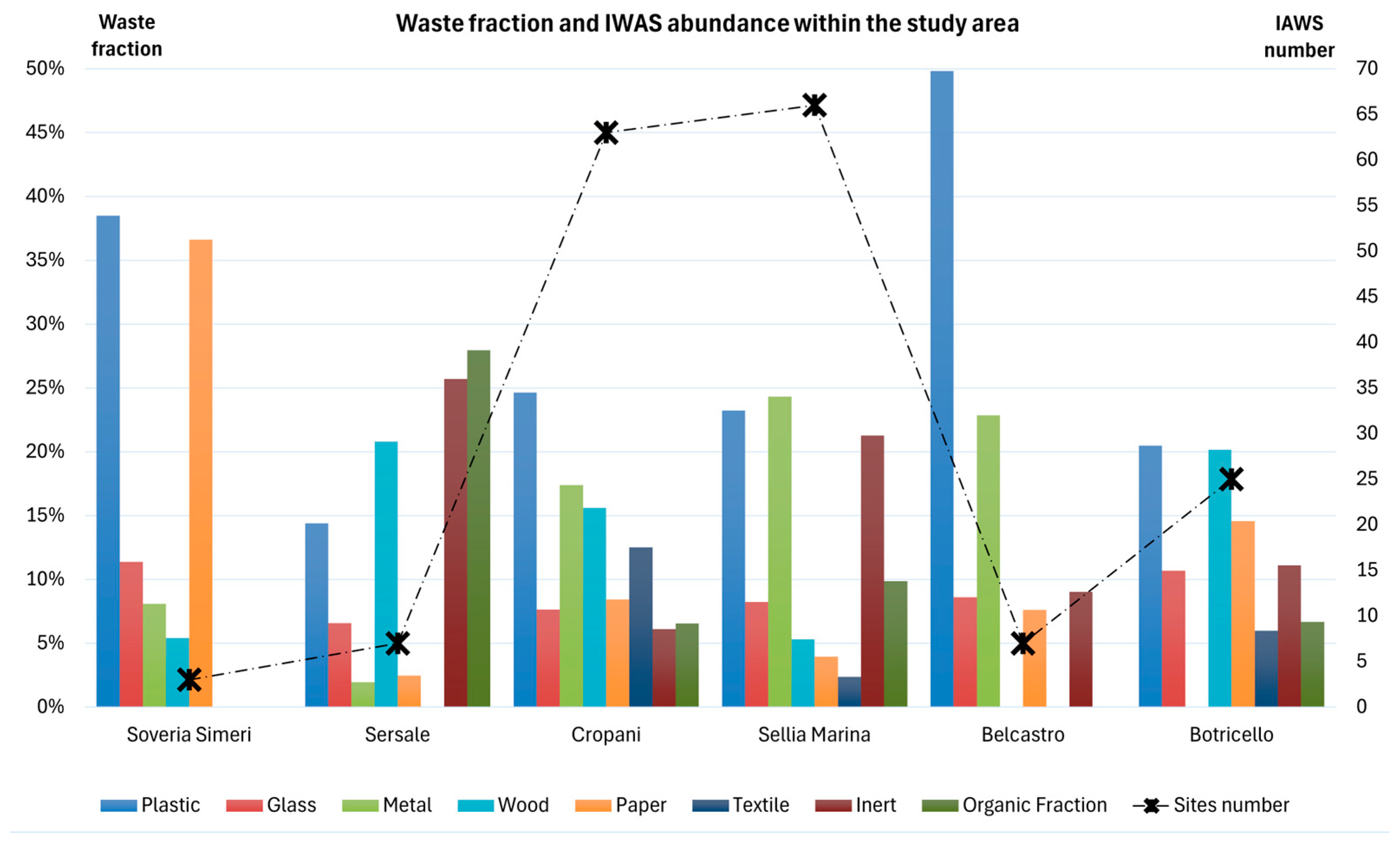
3.2. Ground Investigation

The previous satellite pre-recognition phase across the study area allowed us to pilot the next ground survey.

Figure 9 represents the main layers, highlighting how satellite-based analysis has been helpful to support the ground survey. Accordingly, for a comprehensive overview of the entire IAWSs dataset, in the figure are shown the following main themes:

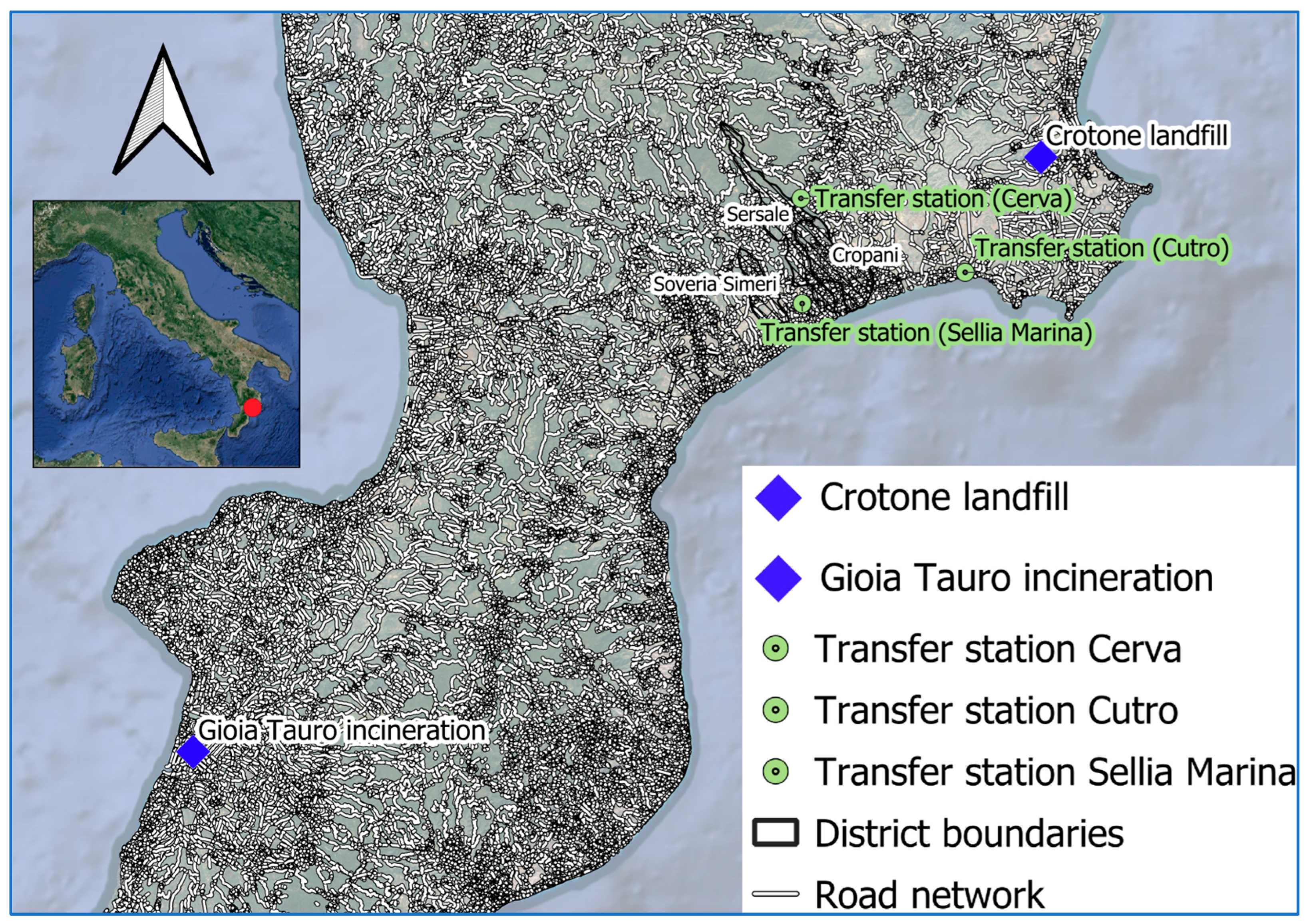
• Sersale, Cropani, and Soveria Simeri districts within the study area (grey line);
• Potential IAWSs recognized by satellite-based analysis (red crosses, transparency 30%);
• IAWSs detected as a result of the ground-based analysis (171 green crosses with a black dot).

Subsequently, from density analysis, two KDF maps have been generated, offering a comprehensive knowledge about IAWS distribution across the study area. By calculating point and volume densities, the two KDF maps reveal critical zones where IAWSs are most concentrated (points and volumes), thus supporting waste management planning. KDF maps can highlight primary regions where IAWSs are concentrated in points and in volumes, suggesting a significant clustering of illegal waste disposal activities (Figure 10 and Figure 11). The density calculation, which factors in the proximity of IAWSs within an 8000 m radius, facilitates the identification of these hotspots area. The presence of these dense clusters indicates areas where illegal dumping is more frequent and/or abundant, likely driven by a combination of accessibility, lack of surveillance, and influence of nearby transportation routes. The distribution of these high-density zones, described also by the contour lines (point and volume densities), could suggest the role of road networks and urban and rural areas in enabling the abandonment of waste.

As shown in Figure 9, the KDF point density map reveals high values in the south-eastern part of the study area, characterized by the presence of an urban area with closely spaced buildings and relatively nearby to the seasonal-use houses in the vicinity of the coastline. In addition, the volumetric analysis conducted from the ground investigation and spatial data analysis offers further insights into the environmental impact of the IAWSs. By estimating the volume of waste at each site, derived from the areal extent and average height of waste piles, the analysis provides an understanding of the illegal dumping activities.

The KDF point density map overlaid with volumetric data reveals that regions with high point densities do not necessarily correspond to areas with significant waste volumes. This correlation underscores the challenge in these areas, suggesting that the high frequency of low-volume illegal waste abandonment occurs in urban areas, while high-volume illegal waste abandonment occurs mainly in rural areas (Figure 11).

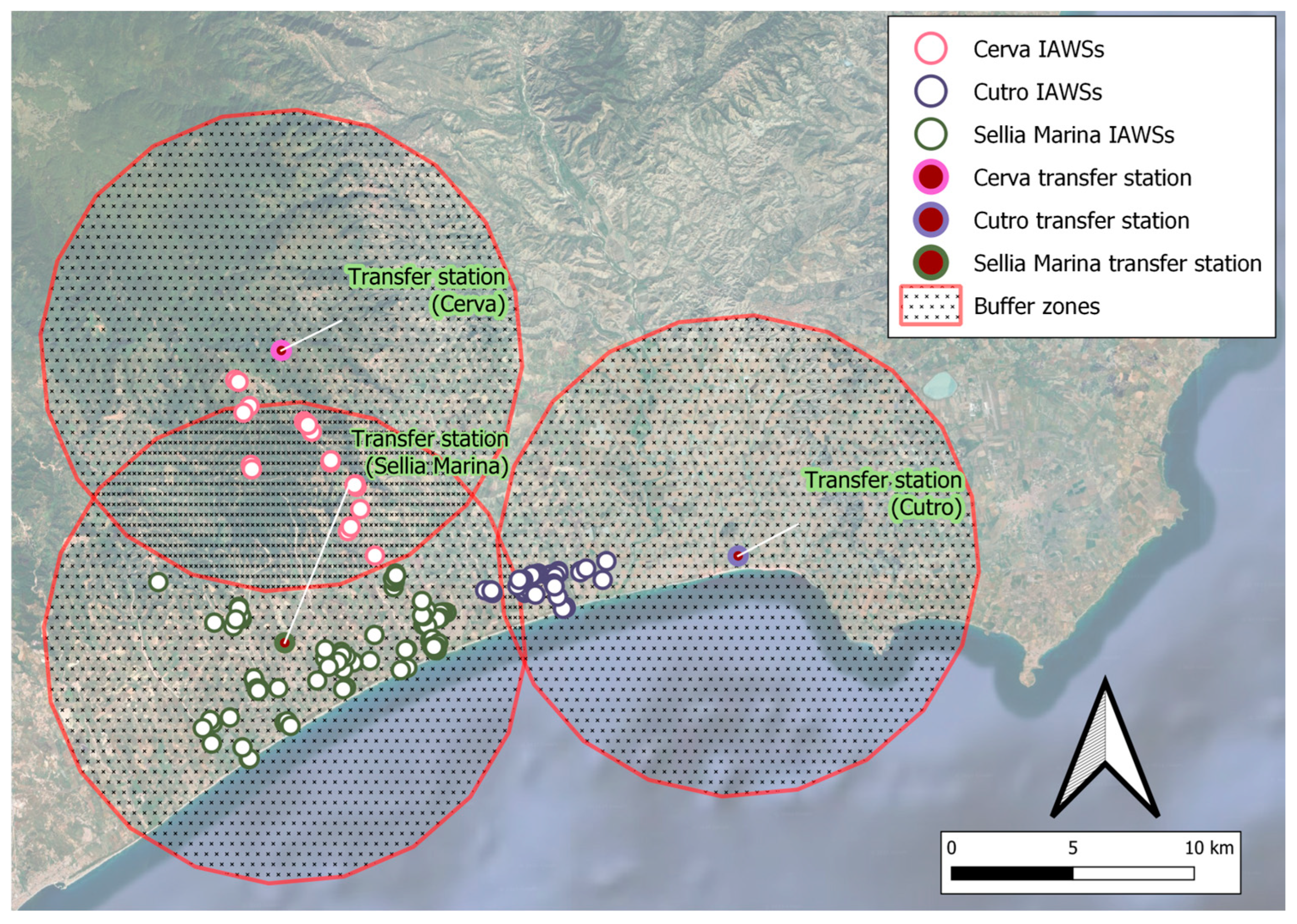
3.3. Application of Dijkstra’s Algorithm in a GIS Environment for Waste Transport Planning

This section presents the findings derived from the application of Dijkstra’s algorithm within a GIS environment for optimizing waste collection, contributing to more sustainable and cost-effective waste management planning. By leveraging the “Shortest Path (point to layer)” tool from QGIS, the analysis provides an examination of the waste management system based on the Calabrian road network, focusing on travel time reduction and fuel consumption optimization. The results are structured to outline the spatial distribution of the IAWSs in relation to the three selected transfer stations. Hence, on the overall efficiency of waste collection, the spatial analysis is characterized by an assessment of the shortest route path determined by the algorithm, highlighting the impact of various route calculation parameters, such as vehicle speed and road network attributes. Initially, the spatial analysis of the study area provides a clear visualization of the key elements involved in the waste management system, including the provincial capitals, disposal plants, and transfer stations.

Figure 12 highlights the strategic placement of the three transfer stations (Cerva, Cutro, and Sellia Marina), each of which is surrounded by a 10 km-radius buffer zone, represented by a red circumference. These buffer zones (red circumferences) delineate the area of responsibility for each transfer station, ensuring an appropriate management of the IAWSs and illustrating the effectiveness of the spatial division for covering the area of interest. Additionally, in the zone of overlap between Cerva and Sellia Marina, the IAWSs located within the transitional area are assigned to the Cerva transfer station. This decision aims to reduce the workload on the Sellia Marina transfer station, which is supposed to manage a significant number of sites. The same reasoning is applied to the smaller disputed area between Cutro and Sellia Marina.

As shown in Figure 13, each designated 10 km-radius buffer area corresponds to the following number of identified IAWSs:

• Cutro transfer station area: 41 IAWSs;
• Sellia Marina transfer station area: 102 IAWSs;
• Cerva transfer station area: 28 IAWSs.

Likewise, once the waste is delivered to the transfer stations, it is further organized and transported to the final disposal and/or treatment plant. Thus, waste can be allocated for landfilling (Crotone plant) and/or for the thermal treatment plant (Gioia Tauro incineration). The optimized routes calculated by using Dijkstra’s algorithm ensure that these subsequent transportation steps are also as efficient as possible, reducing overall operational costs and environmental impacts. The planning of waste collection from IAWSs is described as follows. The distance between each IAWS point and the destination vector layer is determined as distance in meters, calculating the shortest path between the starting points and the final vector layer. Settings are adjusted to influence the route calculation by specifying attributes of the vector data (e.g., speed, topological tolerances, choice of certain roads) and adapting the parameters of the search algorithm for obtaining results that best suit the operator’s needs.

Accordingly, in Figure 14 the following themes are represented:

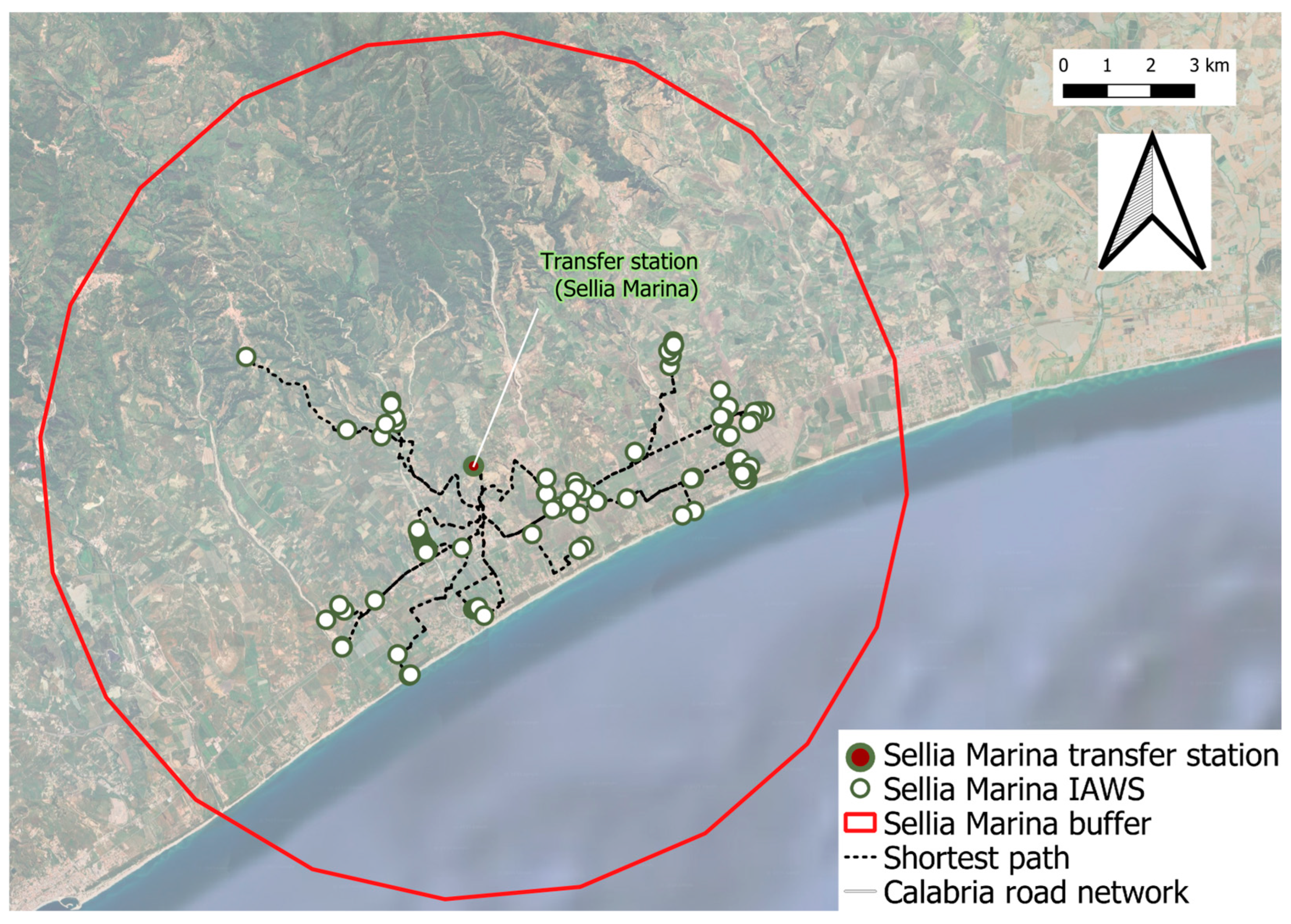
• Sellia Marina transfer station (green and red dot);
• Sellia Marina IAWSs identified as a result of the ground-based analysis (green and white dots);
• Shortest path Sellia Marina (black dashed lines);
• Sellia Marina transfer station buffer zone (red circumference).

Figure 15 reports the following themes:

• Cerva transfer station (pink and red dot);
• Cerva IAWSs identified as a result of the ground-based analysis (pink and white dots);
• Shortest path (black dashed lines);
• Buffer zone (red circumference).

In Figure 16 the following themes are represented:

• Cutro transfer station (violet and red dot);
• Cutro IAWSs identified as a result of the ground-based analysis (violet and white dots);
• Shortest path (black dashed lines);
• Buffer zone (red circumference).

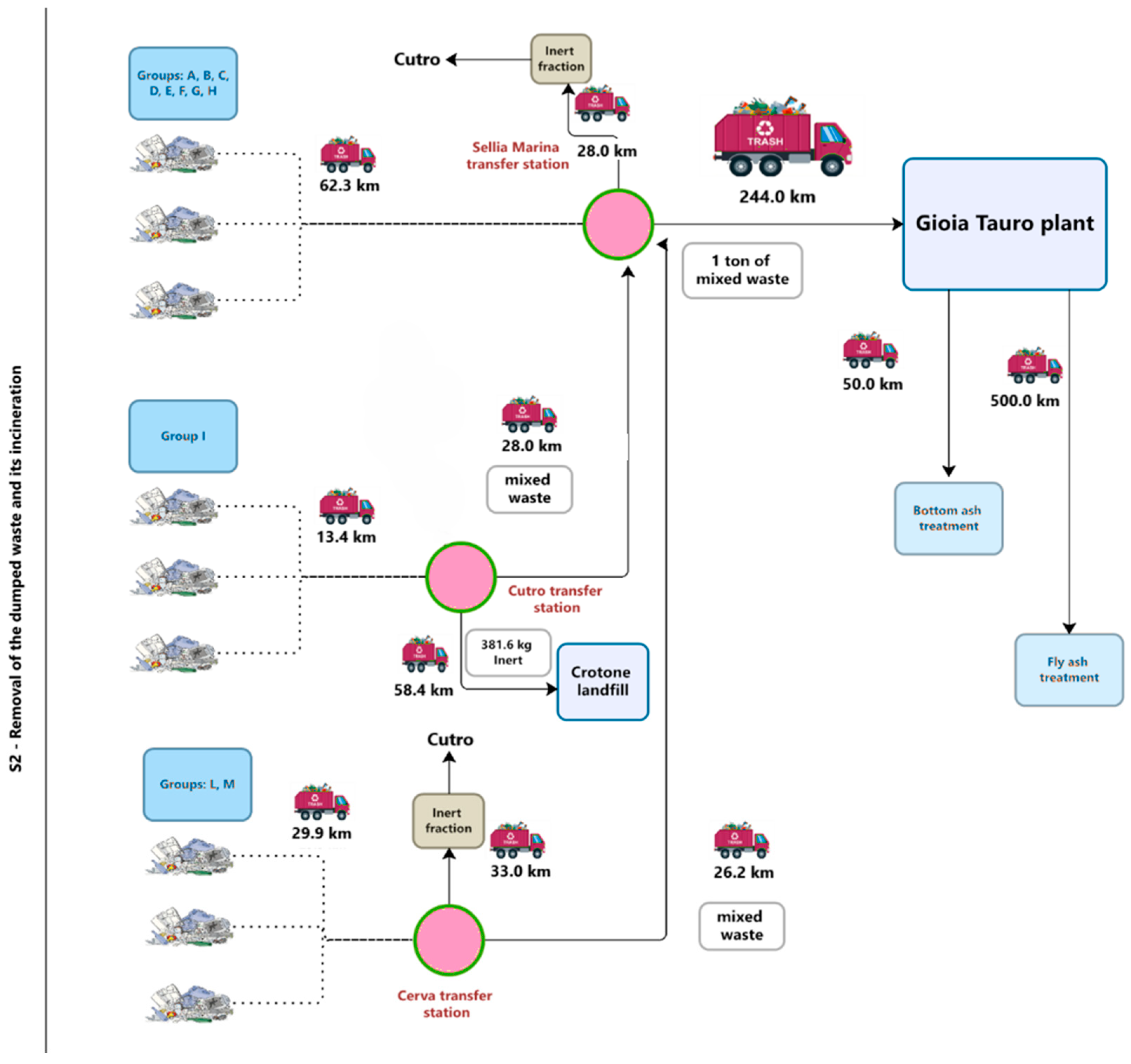
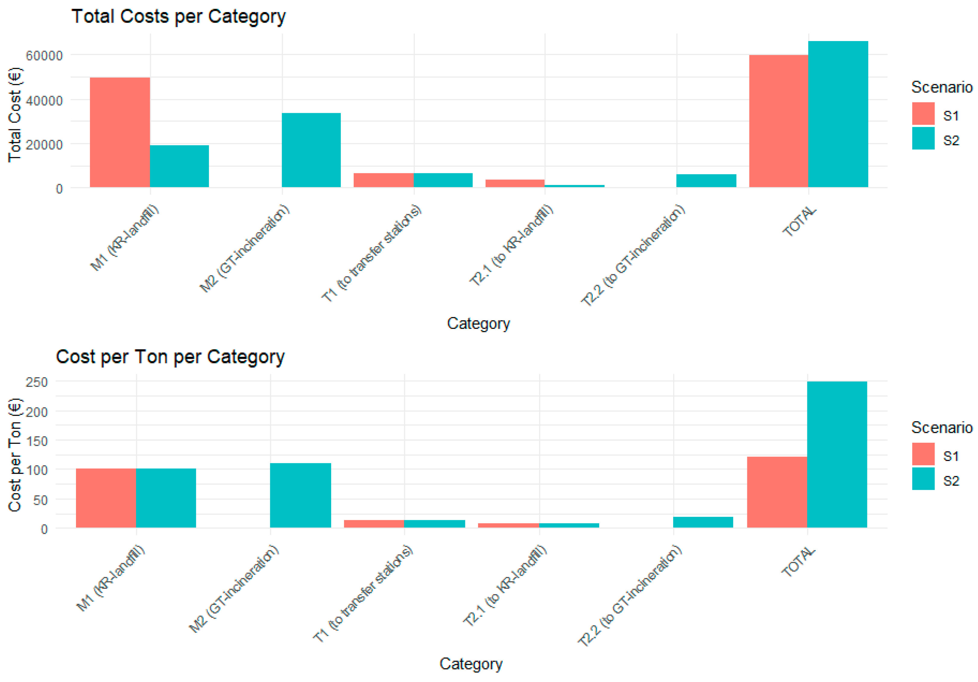
3.4. Cost Analysis Models

For the municipalities involved in this study, IAWSs are identified and managed with the aim of reducing the environmental impacts on natural areas caused by illegal dumping. To achieve this, a cost analysis is applied in the context of waste management planning. Thus, to assess the cost analysis, two scenarios are analyzed: (S1) removal of the illegally dumped waste and disposal at the landfill plant (Crotone) and (S2) removal of the illegally dumped waste and disposal at the incineration plant (Gioia Tauro).

Table 4. Summary of the waste collection distances, areas occupied by waste sites, mass by subgroup (each single group, total mixed waste, inert material), and transfer station affiliation.

Transfer Station	Group	Single Trip Distance (km)	Polygon (m2)	Volume (m3)	Total Mass (kg)
Sellia Marina	A	13.2	36.2	10.7	19,251
	B	3.7	215.2	87.5	158,544
	C	8.1	25.8	1.7	3034
	D	6.9	61.6	1.8	4058
	E	4.4	55.7	15.4	8902
	F	9.1	656.3	46.8	44,038
	G	9.6	169.0	61.0	53,787
	H	7.4	142.0	22.2	24,593
Cutro	I	13.4	651.7	57.5	44,403
Cerva	L	14.2	669.6	184.1	116,265
	M	15.7	248.8	25.5	17,778
Total		105.6	2932.0	514.2	494,650

presents the real values for each IAWS subgroup within the related transfer station buffer zone, indicating group affiliation, area occupied by waste sites (polygon), mean volume, total mass (kg), mixed waste with no inert contribution (kg), and total inert contribution (kg). Accordingly, 11 subgroups have been identified based on proximity, grouping together nearby IAWSs and optimizing the collection process. The assumption is that collection within each subgroup can be completed in a single trip. This strategy allows for an efficient and realistic estimation of travel distances, which is crucial for cost analysis in waste management planning.

S1—Removal of Dumped Waste and Its Disposal in a Landfill

In this scenario, each IAWS is identified through the field surveys, collected, and transported to the Crotone landfill. Initially, waste collected from IAWSs is transported to one of the three transfer stations, each managing waste within a 10 km radius. From these transfer stations, the waste is further consolidated at the Cutro station before being transported to the Crotone landfill for final disposal. The waste sent to the landfill corresponds to 1 ton of mixed waste plus 381.6 kg of inert material per 1 ton of waste, as defined by the FU (

Table 5. Total amount of waste components relative to the FU (1 ton plus 381.6 kg of inert) [27].

Components	Weight (Per 1 Ton of Waste)
Paperboard	104.2 kg
Plastic material	468.6 kg
Glass	148.7 kg
Aluminum	13.9 kg
Scrap steel	150.5 kg
Wood waste	86.9 kg
Textile waste	27.1 kg
Inert material	381.6 kg

).

Specific distance values, detailing the routes from each IAWS to the final disposal site at the landfill, are provided in Figure 17.

S2—Removal of Dumped Waste and Its Incineration

In Scenario 2, the waste collected from each IAWS is transported to the same transfer stations (Sellia Marina, Cutro, and Cerva) used in Scenario 1. As in Scenario 1, the inert fraction, 381.6 kg per ton of waste, is managed similarly to Scenario 1, being stored at the Cutro transfer station and then sent to the Crotone landfill for the final disposal.

However, unlike Scenario 1, the mixed waste, instead of being sent to the Crotone landfill, is further transported to the Gioia Tauro incineration plant (Figure 18). In detail, the transport requirements in the S2 are more complex than in S1, with the mixed waste being collected from Cerva and Cutro and consolidated at the Sellia Marina transfer station before being transported to the Gioia Tauro incineration plant. For the S1 waste management section, all the waste is disposed of in the landfill, while for S2, the inert fraction is sent to the landfill and the mixed fraction to the incineration plant.

Finally,

Table 6. Final costs for Scenario 1 (Crotone-KR landfill) and Scenario 2 (Gioia Tauro-GT incineration).

CATEGORY		S1		S2
		€	€/ton	€	€/ton
Transport	T1 (to transfer stations)	6307.4	12.8	6307.4	12.8
	T2.1 (to KR-landfill)	3629.8	7.3	1337.3	7.1
	T2.2 (to GT-incineration)			5725.4	18.7
Management	M1 (KR-landfill)	49,465.0	100.0	18,875.6	100.0
	M2 (GT-incineration)			33,648.4	110.0
Total		€	€/ton	€	€/ton
		59,402.2	120.1	65,894.1	248.6

reports the final costs for waste management in S1 and S2, considering both total expenditure and cost per ton of waste.

The analysis evaluates transportation costs (T1, T2.1, T2.2), management costs (M1, M2), and overall total costs. The transportation costs are defined as follows:

-

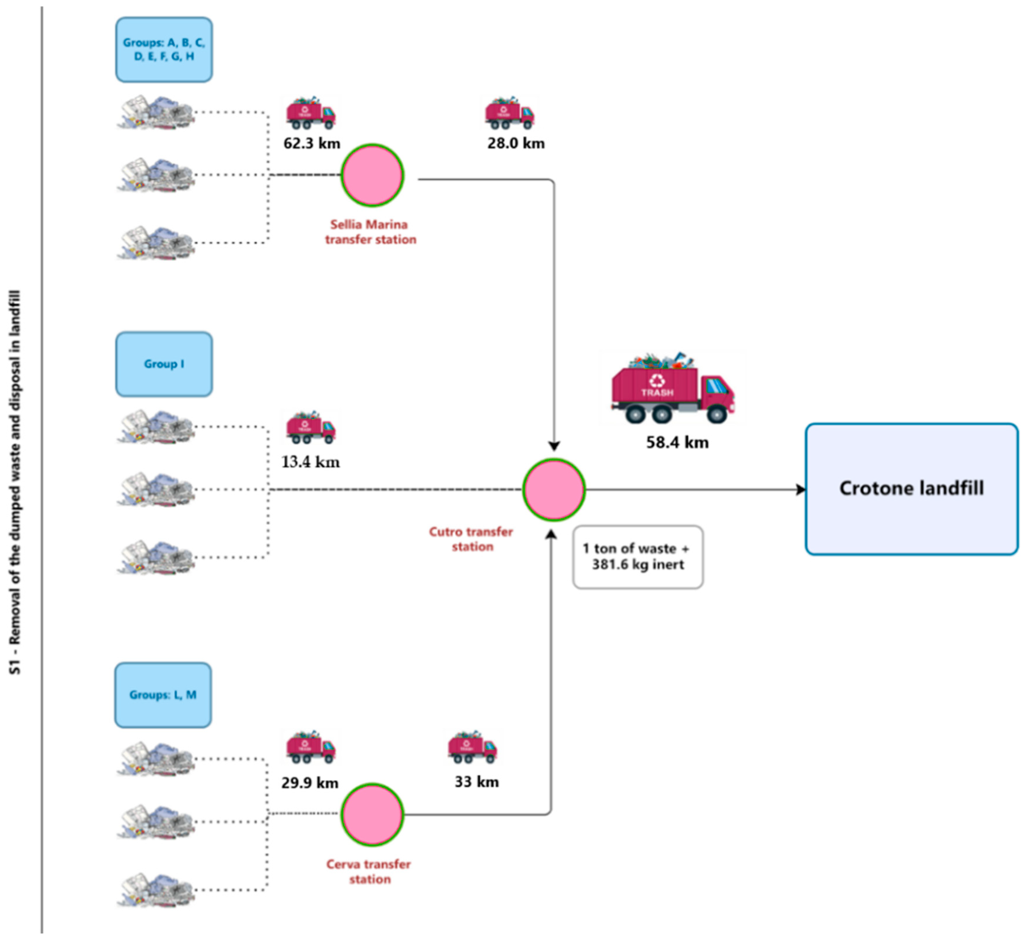
T1: the transportation cost from dumpsites to transfer stations is the same for both scenarios (€6307.4 or €12.8/ton).

-

T2.1: the cost of transporting waste to the Crotone landfill in Scenario 1 (€3629.8 or €7.3/ton) is lower than the equivalent cost in S2 for inert waste (€7.1/ton), as S2 reduces the amount of waste transported due to separation.

-

T2.2: Scenario 2 incurs additional transportation costs (€5725.4 or €18.7/ton) due to the transport of mixed waste to the Gioia Tauro plant.

The management costs are estimated as follows:

-

M1: landfill disposal costs are significantly higher in S1 (€49,465.0 or €100.0/ton) than in S2 (€18,875.6 or €100.0/ton), as S2 only disposes of the inert fraction in the landfill.

-

M2: incineration costs in S2 (€33,648.4 or €110.0/ton) can replace full landfill disposal, offering energy recovery as a benefit.

4. Discussion

This study assesses the hypothetical costs associated with Illegal Abandoned Waste Sites (IAWSs) management by using a GIS-based framework for two scenarios: landfill and incineration plants. Compared to previous studies [12,16,17,18,21,22,35,36,37,38,39,40,41,42,43,44,45,46,47,48,49], this research provides an integrated approach that comprises remote sensing, street-level verification, ground surveys, product and 2.5D volume analyses, GIS-based computational analysis, Python scripts, and cost analysis modeling. As mentioned above, GISs are often used in solid waste management to link spatial contents and planning strategies, dealing with times and costs for optimizing waste collection and transportation. Accordingly, insights are provided for regional planning and policymaking, suggesting needs for additional facilities, improvements in road connectivity, and sustainable practices in the region for different scenarios. In this research, a GIS-based framework is needed for outlining optimal routes to detect, collect, transport, and manage IAWSs. As in other studies [24,25,26,27,28,29,30,31,32,33,34,35,36,37,38,39], ancillary data collection was derived from various sources. Consequently, in this work, optimal and less time- and cost-intensive routes are defined by using a GIS-based framework and Python algorithms. This multi-parametric GIS-based approach not only supports the spatial mapping of waste sites but also underpins the final cost analysis assessment by estimating waste composition and optimizing waste transport logistics. Thus, this integrated methodology, which combine GPS data, photointerpretation, and product analysis, can offer a comprehensive framework for assessing IAWSs characterization within a cost analysis context. It facilitates both the spatial mapping and the quantification of waste, contributing to more effective monitoring and management strategies. Compared to other studies [35,36,37,38,39,40,41,42,43,44,45,46,47,48,49], the innovation of this work lies in the following key points:

(1)

Use of open-source software and an Excel-based scenario;

(2)

Satellite remote sensing as a pre-analysis stage to set ground surveys;

(3)

In-situ ground survey activities for geo-localization refinement and qualitative/quantitative product and 2.5D volume analyses of waste piles;

(4)

Use of ancillary data (primary and secondary road networks, transfer stations, disposal plants) and application of the Dijkstra algorithm (QGIS, Shortest Path tool—point to layer);

(5)

Cost analysis and waste management planning.

An initial analysis using remote sensing was conducted. According to the photo-interpretative analysis, Very High Resolution (VHR) satellite and Google Earth imaging were used to recognize potential IAWSs from both nadiral (Google Earth^® and WorldView-3) and street-level perspectives (Google Street View^®). This pre-analysis phase aimed to qualitatively identify potential contaminated sites by discriminating, from a regional scale, homogeneous areas.

Subsequently, a ground survey was fundamental to identify and verify the occurrence of IAWSs. Hence, several images were obtained from each site (https://github.com/AlfRag91/IAWSs.git), acquiring data for 171 sampling sites. Through photo-interpretative image analysis, various types of materials were identified within the areas of interest, including bulky waste (e.g., washing machines, refrigerators, ovens, TVs, water heaters, furniture, buckets, chairs, mattresses, sofas), paperboard, garbage bags with clear packaging, garbage bags with no clear packaging, construction and demolition waste (e.g., excavated soil, bathroom fixtures, pipes, insulation sheathing, metal sheets, garden trimmings, burned remains). Thus, future work surely will concern the development of algorithms able to detect automatically the material within the illegal waste sites by using photogrammetry, machine learning, and deep learning techniques.

To provide a more comprehensive understanding of the scale of illegal dumping activities across the study area, a 2.5-dimensional volumetric perspective was developed using surface data (QGIS analysis) of the polluted areas and mean waste pile height approximations (ground analysis). Expertise in photointerpretation and Excel-based scenarios enabled the creation of a dataset useful for the final cost analysis assessment. Moreover, by using ancillary data (primary and secondary road networks, transfer stations, disposal plants) and the Dijkstra algorithm (QGIS, Shortest Path tool—point to layer), a shortest route paths layer was obtained for managing distances and transports between each IAWS and disposal plants.

As previously mentioned, to manage all these types of data, a structured Excel-based scenario analysis tool is provided, useful to process and analyze data efficiently (https://github.com/AlfRag91/IAWSs.git). The tool leverages the background data described in the previous sections and provides a structured approach to evaluating waste management scenarios. By incorporating key parameters such as material density, weight distribution, and volume contributions, the tool allows users to assess the impact of different waste disposal strategies. The Excel-based model is designed to be user-friendly, enabling stakeholders to input new data, adjust key variables, and visualize results through automated calculations.

Regarding the cost analysis, the Scenario 1 waste is designed for landfill disposal, where inert materials play a crucial role. Hence, with 381.6 kg of inert waste per 1 ton of mixed waste, this fraction contributes to increased landfill space utilization and requires careful consideration in the environmental assessment. Regarding the total costs values, S1 shows a total cost of €59,402.2 (€120.1/ton). In contrast, Scenario 2 reveals higher total costs, such as €65,894.1 (€248.6/ton), due to the longer transport distances to the incineration plant and additional incineration management costs. Thus, from a purely economic point of view, Scenario 1 is the most cost-effective solution. However, Scenario 2 presents environmental and economic benefits by allowing for energy recovery and metal recycling, aligning with European guidelines on reducing landfill use and maximizing resource recovery. Accordingly, landfilling, while considered a less energy-intensive solution compared to incineration, can generate long-term environmental risks, particularly in terms of land occupation, methane emissions, and potential soil and groundwater contamination. Furthermore, landfills represent a considerable problem in terms of energy recovery, as they eliminate any possibility to recover materials for future applications [9,10,11]. Scenario 2 concerns the incineration plant strategy, allowing for a more energy-efficient process, with the capability for energy recovery. Although this scenario reduces the physical volume of waste, it leaves behind residues such as fly ash, requiring additional disposal strategies. In both scenarios, critical concerns remain regarding human health, freshwater ecotoxicity, and toxicity to humans. Landfilling poses risks of leachate contamination, while incineration results in toxic emissions that can impact air quality if not managed through effective and safe disposal strategies (see https://content.gruppoa2a.it/sites/default/files/2023-05/relazione-annuale-silla-2022.pdf, accessed on 29 January 2025). On the other hand, policy implications for waste management strategies play a crucial role in ensuring sustainable practices and balancing economic feasibility and environmental responsibility. The findings of this study provide insights into the implications of different waste disposal strategies, highlighting the need for targeted policy measures. In accordance with national and European Union (EU) regulations for waste management policies, particularly the EU Waste Framework Directive and the Circular Economy Action Plan, this study aims to improve waste management planning in terms of collection, transport, and disposal. Scenario 2, which involves incineration, is more aligned with these principles, as it promotes energy recovery and reduces landfill dependency. Additionally, strategies to improve waste sorting at the source could further enhance the efficiency of both landfill and incineration solutions. Moreover, the study underscores the need for improving waste management infrastructure to enhance efficiency and minimize environmental impacts.

GIS-based frameworks, as demonstrated in this study, offer policymakers a valuable tool for optimizing waste collection, transportation, and disposal. By integrating spatial data with planning strategies, local authorities can identify high-priority areas for intervention, determine the most efficient waste transport routes, and plan the establishment of additional transfer stations or disposal sites. Regional governments should consider adopting GIS-based waste management planning to improve service efficiency, reduce operational costs, and ensure equitable waste management coverage across different areas.

5. Conclusions

This study highlights the importance of integrated waste management planning systems, considering both collection and transport factors during the appropriate operations. Policymakers should prioritize strategies that reduce waste generation and transport, while enhancing the recycling and recovery of materials to minimize landfill use and the need for incineration. A GIS-based framework can identify Illegal Abandoned Waste Sites (IAWSs), supporting the collection, management, and transportation of waste. Accordingly, the GIS-based framework can serve as a fundamental decision-making tool, applicable in regions like Calabria, where waste abandonment is a persistent issue. In addition, future requirements for waste treatment infrastructure can be planned by considering trends and current spatial distribution. This may involve suggesting locations for new facilities and/or identifying areas where existing infrastructure needs to be upgraded. The integration of Dijkstra’s algorithm, programming languages, GIS software, remote/ground sensing techniques, as well as product and volume analysis, proves useful in optimizing waste collection routes and improving waste management planning. By efficiently calculating the shortest paths from waste sites to transfer stations and final plant disposal, decision-makers can achieve better resource allocation, reducing travel times and relative costs. Hence, the development of a waste management plan requires an understating of shortest paths, product analysis, transfer stations, and disposal plants.

This methodology provides a workflow for informed decision-making regarding the management of disputed areas and the destination of waste. Firstly, through a multi-approach methodology, several activities are carried out by leveraging remote sensing, ground data, and qualitative product and 2.5D volume analyses. This approach enables the identification of conditions in the study area through an initial qualitative estimation of the distribution of abandoned waste.

Figure 19 presents an overview of the different waste materials found in IAWSs across six municipalities: Soveria Simeri, Sersale, Cropani, Sellia Marina, Belcastro, and Botricello. These materials are categorized by percentage weight and include steel, plastic, glass, metal, wood, paper, textiles, inert materials, and organic fractions. Additionally, the figure includes the number of IAWSs associated with each municipality.

Consequently, the quantitative cost analysis is based on costs related to collection and transport activities. This work ensures that the entire waste management process, from collection to final disposal or treatment, is conducted in an optimized and sustainable manner. The comparison between the two scenarios (landfill and incineration) can determine the most appropriate solution in relation to the type of waste material, local conditions, transportation, and further potential long-term impacts.

Both scenarios present viable options for collecting and managing waste from each IAWS, where each has its unique set of advantages and challenges (Figure 20). The Cost per Ton per Category plot highlights the economic differences between landfill disposal (S1) and incineration (S2-G) when normalized on a per-ton basis (Functional Unit). S1 maintains a lower cost per ton (€120.1 €/ton) compared to S2-G (€248.6 €/ton). Regarding the total cost values, S1 and S2 show total costs of €59,402.2 and €65,894.1, respectively. It is important to note that S2 is characterized by incineration management costs and longer transport distances, due to the greater distance to the Gioia Tauro plant. Accordingly, landfill disposal remains the most cost-effective short-term solution, though this does not account for long-term environmental and regulatory implications. The higher costs associated with S2-G are primarily driven by the long distance to the incineration plant and, secondly, by energy recovery operations and the need for specialized residue disposal. Indeed, while incineration reduces waste volume and recovers energy, it generates fly ash and other residues that require additional treatment, adding to the overall cost. As noted earlier, transport costs are higher in S2-G due to the longer distances to incineration facilities, further increasing per-ton expenses.

Despite its higher cost, S2 aligns with European sustainability goals, prioritizing waste-to-energy conversion and landfill reduction. European waste policies encourage resource recovery over direct disposal, viewing landfills as a last resort due to their environmental impact. Over time, the financial burden of landfill management, such as leachate treatment, methane emission control, and land occupation, may render incineration a more attractive alternative. This comparison highlights the trade-off between economic feasibility and environmental sustainability, suggesting that future waste management strategies must balance short-term cost efficiency with long-term ecological responsibility.

In conclusion, Scenario 1, focused on landfill disposal, is simpler logistically but is characterized by higher environmental costs due to long-term landfill impacts. Scenario 2, with its incineration approach, reduces landfill usage and can potentially recover energy, although it introduces higher operational complexity and costs. The Circular Economy framework, as a decision-support tool for municipal solid waste management, can be used to help identify the best trade-offs involved in more sustainable practices. Accordingly, this study has successfully provided a GIS-based framework to detect and manage IAWSs, which can be implemented at both local and regional scales. Key outcomes include the assessment of cost analysis within a circular economic context; the improvement of waste management planning; the enhancement of decision-support tools through LCA studies; and the promotion of community awareness to reduce the abandonment of waste in the territory.

Our future perspective considers: (1) improving image classification for IAWS detection; (2) improving the accuracy of volumetric analysis by using Unmanned Aerial Vehicle (UAV) imagery; (3) performing a Life Cycle Assessment; and (4) incorporating the topographical variable into the cost analysis model. Indeed, LCA applications, in relation to this study, can serve as a helpful tool for selecting more sustainable waste management operations.

References

1. Wenheng, W.; Shuwen, N. Impact study on human activity to the resource-environment based on the consumption level difference of China’s Provinces or autonomous regions. China Popul. Resour. Environ. 2008, 18, 121–127. [Google Scholar] [CrossRef]
2. Salami, L.; Popoola, L.T. A comprehensive review of atmospheric air pollutants assessment around landfill sites. Air Soil Water Res. 2023, 16, 11786221221145379. [Google Scholar] [CrossRef]
3. Giusti, L. A Review of Waste Management Practices and Their Impact on Human Health. Waste Manag. 2009, 29, 2227–2239. [Google Scholar] [CrossRef] [PubMed]
4. Karimi, N.; Ng, K.T.W.; Richter, A. Development and application of an analytical framework for mapping probable illegal dumping sites using nighttime light imagery and various remote sensing indices. Waste Manag. 2022, 143, 195–205. [Google Scholar] [CrossRef]
5. Jakiel, M.; Bernatek-Jakiel, A.; Gajda, A.; Filiks, M.; Pufelska, M. Spatial and temporal distribution of illegal dumping sites in the nature protected area: The Ojców National Park, Poland. J. Environ. Plan. Manag. 2019, 62, 286–305. [Google Scholar] [CrossRef]
6. Jiang, P.; Fan, Y.V.; Zhou, J.; Zheng, M.; Liu, X.; Klemeš, J.J. Data-driven analytical framework for waste-dumping behaviour analysis to facilitate policy regulations. Waste Manag. 2020, 103, 285–295. [Google Scholar] [CrossRef]
7. Ghosh, A.; Richter, A.; Ng, K.T.W. Applications of Geographic Information Systems to site waste facilities in Saskatchewan—Phase. In Proceedings of the Canadian Society of Civil Engineering Annual Conference 2021, Lecture Notes in Civil Engineering, Ottawa, ON, Canada, 14–17 June 2011; Volume 249, pp. 173–182. [Google Scholar]
8. Quesada-Ruiz, L.C.; Rodriguez-Galiano, V.; Jordá-Borrell, R. Characterization and mapping of illegal landfill potential occurrence in the Canary Islands. Waste Manag. 2019, 85, 506–518. [Google Scholar] [CrossRef]
9. Yadav, R.; Sahu, L.K.; Jaaffrey, S.N.A.; Beig, G. Temporal Variation of Particulate Matter (PM) and Potential Sources at an Urban Site of Udaipur in Western India. Aerosol Air Qual. 2014, 14, 1613–1629. [Google Scholar] [CrossRef]
10. Mahmood, K.; Batool, S.A.; Chaudhry, M.N. Studying bio-thermal effects at and around MSW dumps using Satellite Remote Sensing and GIS. Waste Manag. 2016, 55, 118–128. [Google Scholar] [CrossRef]
11. Karimi, N.; Richter, A.; Ng, K.T.W. Siting and ranking municipal landfill sites in regional scale using nighttime satellite imagery. J. Environ. Manag. 2020, 256, 109942. [Google Scholar] [CrossRef]
12. Papale, L.G.; Guerrisi, G.; De Santis, D.; Schiavon, G.; Del Frate, F. Satellite Data Potentialities in Solid Waste Landfill Monitoring: Review and Case Studies. Sensors 2023, 23, 3917. [Google Scholar] [CrossRef] [PubMed]
13. Ottavianelli, G.; Hobbs, S.; Smith, R.; Bruno, D. Assessment of Hyperspectral and SAR Remote Sensing for Solid Waste Landfill Management; European Space Agency: Frascati, Italy, 2005; (Special Publication) ESA SP. [Google Scholar]
14. Gemitzi, A.; Tsihrintzis, V.A.; Voudrias, E.; Petalas, C.; Stravodimos, G. Combining geographic information system, multicriteria evaluation techniques and fuzzy logic in siting MSW landfills. Environ. Geol. 2007, 51, 797–811. [Google Scholar] [CrossRef]
15. Richter, A.; Ng, K.T.W.; Karimi, N.; Chang, W. Developing a novel proximity analysis approach for assessment of waste management cost efficiency in low population density regions. Sustain. Cities Soc. 2021, 65, 102583. [Google Scholar] [CrossRef]
16. Singh, G.; Singh, B.; Rathi, S.; Haris, S. Solid Waste Management using Shortest Path Algorithm. Int. J. Eng. Sci. Invent. Res. Dev. 2014, 1, 60–64. [Google Scholar]
17. Maspaitella, B.J.; Susanty, A.; Purwaningsih, R. Waste transportation route garbage using network analysis method, a research method design. IOP Conf. Ser. Mater. Sci. Eng. 2021, 1072, 012025. [Google Scholar] [CrossRef]
18. Mati Asefa, E.; Bayu Barasa, K.; Adare Mengistu, D. Application of Geographic Information System in Solid Waste Management; IntechOpen: London, UK, 2022. [Google Scholar]
19. Dijkstra, E.W. A note on two problems in connection with graphs. Numer. Math. 1959, 1, 269–271. [Google Scholar] [CrossRef]
20. Hannan, M.A.; Begum, R.A.; Al-Shetwi, A.Q.; Ker, P.J.; Al Mamun, M.A.; Hussain, A.; Basri, H.; Mahlia, T.M.I. Waste collection route optimisation model for linking cost saving and emission reduction to achieve sustainable development goals. Sustain. Cities Soc. 2020, 62, 102393. [Google Scholar] [CrossRef]
21. Kontos, T.D.; Komilis, D.P.; Halvadakis, C.R. Siting MSW landfills on Lesvos Island with a GIS-based methodology. Waste Manag. Res. 2003, 21, 262–277. [Google Scholar] [CrossRef]
22. Cleary, J. The incorporation of waste prevention activities into life cycle assessments of municipal solid waste management systems: Methodological issues. Int. J. Life Cycle Assess. 2010, 15, 579–589. [Google Scholar] [CrossRef]
23. ISPRA. Municipal Waste Report—2022 (Edition 355/2021); ISPRA: Rome, Italy, 2022.
24. Liang, J.; Gong, J.; Li, W. Applications and impacts of Google Earth: A decadal review (2006–2016). ISPRS J. Photogramm. Remote Sens. 2018, 146, 91–107. [Google Scholar] [CrossRef]
25. Biljecki, F.; Ito, K. Street view imagery in urban analytics and GIS: A review. Landsc. Urban Plan. 2021, 215, 104217. [Google Scholar] [CrossRef]
26. Carper, W.; Lillesand, T.M.; Kiefer, R.W. The use of Intensity-Hue-Saturation transformations for merging SPOT panchromatic and multispectral image data. Photogramm. Eng. Remote Sens. 1990, 56, 1067–1074. [Google Scholar]
27. WEEE Coordination Center. Available online: https://www.cdcraee.it/ (accessed on 29 March 2024).
28. Agbogbloshie Makerspace Platform (AMP). Available online: https://qamp.net/library/microwave-ovens/ (accessed on 29 March 2024).
29. Zero Waste Europe. Available online: http://zerowastecities.eu (accessed on 29 March 2024).
30. International Atomic Energy Agency (IAEA). Available online: http://www-pub.iaea.org (accessed on 29 March 2024).
31. Manea, A.; Dolci, G.; Grosso, M. Life cycle assessment and cost analysis of an innovative automatic system for sorting municipal solid waste: A case study at Milan Malpensa airport. Waste Manag. 2024, 183, 63–73. [Google Scholar] [CrossRef] [PubMed]
32. Ministry of Infrastructure and Transport Data. 2022. Available online: https://www.mit.gov.it/ (accessed on 29 March 2024).
33. Ministry of Ecological Transition. 2022. Available online: https://sisen.mase.gov.it/dgsaie/ (accessed on 29 March 2024).
34. Steubing, B.; Wernet, G.; Reinhard, J.; Bauer, C.; Moreno-Ruiz, E. The ecoinvent database version 3 (part II): Analyzing LCA results and comparison to version 2. Int. J. Life Cycle Assess. 2016, 21, 1269–1281. [Google Scholar] [CrossRef]
35. Mei, A.; Baiocchi, V.; Mattei, S.; Zampetti, E.; Pai, H.-J.; Tratzi, P.; Ragazzo, A.V.; Cuzzucoli, A.; Mancuso, A.; Bearzotti, A.; et al. Conceptualization of a satellite, UAS and UGV downscaling approach for abandoned waste detection and waste to energyprospects. Int. Arch. Photogramm. Remote Sens. Spat. Inf. Sci. 2023, 26, 287–293. [Google Scholar] [CrossRef]
36. Ghose, M.K.; Dikshit, A.K.; Sharma, S.K. A GIS-based transportation model for solid waste disposal—A case study on Asansol municipality. Waste Manag. 2006, 26, 1287–1293. [Google Scholar] [CrossRef]
37. Malakahmad, A.; Bakri, P.M.; Mokhtar, M.R.; Khalil, N. Solid Waste Collection Routes Optimization via GIS Techniques in Ipoh City, Malaysia. Procedia Eng. 2014, 77, 20–27. [Google Scholar] [CrossRef]
38. Hatamleh, R.I.; Jamhawi, M.M.; Al-Kofahi, S.D.; Hijazi, H. The Use of a GIS System as a Decision Support Tool for Municipal Solid Waste Management Planning: The Case Study of Al Nuzha District, Irbid, Jordan. Procedia Manuf. 2020, 44, 189–196. [Google Scholar] [CrossRef]
39. Baral, A.; Rafizul, I.M.; Das, S.; Bernar, S. Economic and environmental benefits of optimized waste transportation routes in Khulna. Environ. Chall. 2024, 17, 101023. [Google Scholar] [CrossRef]
40. Deswal, M.; Laura, J.S. Application of GIS in MSW management in India. Int. J. Eng. Res. Dev. 2014, 10, 24–32. [Google Scholar]
41. Khajuria, A.; Matsui, T.; Machimura, T. GIS Application for Estimating the Current Status of Municipal Solid Waste Management System: Case Study of Chandigarh City, India. Our Nat. 2012, 9, 26–33. [Google Scholar] [CrossRef]
42. Siddam, S.; Khadikar, I.; Chitade, A.Z. Route Optimisation for Solid Waste Management Using Geo-Informatics. IOSR J. Mech. Civ. Eng. 2012, 2, 78–83. [Google Scholar] [CrossRef]
43. Goel, S. Advances in Solid and Hazardous Waste Management; Springer: Cham, Switzerland, 2017. [Google Scholar]
44. Li, X.; Zhang, C.; Li, W.; Ricard, R.; Meng, Q.; Zhang, W. Assessing street-level urban greenery using Google Street View and a modified green view index. Urban For. Urban Green. 2015, 14, 675–685. [Google Scholar] [CrossRef]
45. Kang, Y.; Zhang, F.; Gao, S.; Lin, H.; Liu, Y. A review of urban physical environment sensing using street view imagery in public health studies. Ann. GIS 2020, 26, 261–275. [Google Scholar] [CrossRef]
46. Cicala, L.; Gargiulo, F.; Parrilli, S.; Amitrano, D.; Pigliasco, G. Progressive Monitoring of Micro-Dumps Using Remote Sensing: An Applicative Framework for Illegal Waste Management. Sustainability 2024, 16, 5695. [Google Scholar] [CrossRef]
47. Syafrudin, S.; Ramadan, B.S.; Budihardjo, M.A.; Munawir, M.; Khair, H.; Rosmalina, R.T.; Ardiansyah, S.Y. Analysis of Factors Influencing Illegal Waste Dumping Generation Using GIS Spatial Regression Methods. Sustainability 2023, 15, 1926. [Google Scholar] [CrossRef]
48. Ichipi, E.B.; Senekane, M.F. An Evaluation of the Impact of Illegal Dumping of Solid Waste on Public Health in Nigeria: A Case Study of Lagos State. Int. J. Environ. Res. Public Health 2023, 20, 7069. [Google Scholar] [CrossRef]
49. Ngalo, N.; Thondhlana, G. Illegal Solid-Waste Dumping in a Low-Income Neighbourhood in South Africa: Prevalence and Perceptions. Int. J. Environ. Res. Public Health 2023, 20, 6750. [Google Scholar] [CrossRef]
Figure 1. Flowchart of the present study. The waste management planning concerns an initial analysis by using ancillary data and remote sensing instruments. In the end, by using Dijkstra’s algorithm in a GIS environment, a shortest path analysis is provided from ground data, obtaining shortest paths between IAWSs and disposal points, aiming to finalize cost analysis models.
Earth 06 00033 g001
Figure 2. Municipalities’ waste collection during the year 2021 [23].
Earth 06 00033 g002
Figure 3. Ancillary data considered in this study. In blue are represented the waste plants (Gioia Tauro incineration and Crotone landfill); in green the transfer stations (Cerva, Cutro, Sellia Marina); in white municipal districts (Sersale, Soveria Simeri, Cropani). Municipality administrative borders are represented in grey. Basemap: Google Satellite.
Earth 06 00033 g003
Figure 4. Representation of the basic geometric approximation (rectangular cuboid) for each IAWS.
Earth 06 00033 g004
Figure 5. This image shows the presence of an IAWS in the municipality of Cropani. On the right, the top panel displays a WorldView (pansharpening results, July 2021) satellite image along with geospatial data from ground and remote sensing. The bottom panel presents the results of the qualitative product and 2.5D volume analyses. On the left, two images related to Site O3 are shown.
Earth 06 00033 g005
Figure 6. Integrated waste management workflow: from data collection to transport optimization and disposal strategy.
Earth 06 00033 g006
Figure 7. Identification of potential IAWSs in the municipality of Cropani through satellite and street-level pre-recognition analysis. The three images are described as follows: (a) Pansharpening results from WorldView-3 image (July 2021) for the study area; (b) image from Google Earth platform (May 2021); (c) image from Google Street View (April 2021).
Earth 06 00033 g007
Figure 8. KDF map obtained from satellite monitoring and photointerpretation activities. Red crosses represent the locations of identified IAWSs. Basemap: Google Satellite.
Earth 06 00033 g008
Figure 9. Representation of IAWS evidence in the study area lying within the municipalities. The map’s features are denoted as follow: municipality administrative borders in grey; IAWS satellite points by red crosses; IAWS ground points by green crosses with a central black dot.
Earth 06 00033 g009
Figure 10. Representation of the KDF point density map based on ground investigation. Ground IAWS evidence across the study area is concentrated within an urban area near the coastline.
Earth 06 00033 g010
Figure 11. Representation of the KDF volume density map based on ground investigation. Ground IAWS evidence across the study area is concentrated within a rural area near the coastline.
Earth 06 00033 g011
Figure 12. Map of the study area representing the provincial cities, disposal plants, the three transfer stations (Cerva, Cutro, Sellia Marina), and the 10 km-radius buffer areas surrounding each transfer station. Red circles denote areas managed by each transfer station.
Earth 06 00033 g012
Figure 13. Map of the study area illustrating the following elements: IAWS points identified by ground survey activities, with the assigned transfer station (Cutro, Cerva, Sellia Marina) represented by colored circles filled with white; transfer station, represented by colored circles (Cerva, Cutro, Sellia Marina); 10 km-radius buffer designated areas (red circumference filled with dots).
Earth 06 00033 g013
Figure 14. Map of the study area illustrating ancillary data (Sellia Marina transfer station); ground-based IAWSs identified across the study area; layers and results for the shortest path analysis (buffer zone and shortest path route layer).
Earth 06 00033 g014
Figure 15. Map of the study area illustrating ancillary data (Cerva transfer station); ground-based IAWSs identified across the study area; layers and results for the shortest path analysis (buffer zone and shortest path route layer).
Earth 06 00033 g015
Figure 16. Map of the study area illustrating ancillary data (Cutro transfer station); ground-based IAWSs identified across the study area; layers and results for the shortest path analysis (buffer zone and shortest path route layer).
Earth 06 00033 g016
Figure 17. Representation of the S1 system boundaries. Bizagi Modeler open-source software is used to create the scenario.
Earth 06 00033 g017
Figure 18. Representation of the S2 system boundaries. Bizagi Modeler open-source software is used to create the scenario.
Earth 06 00033 g018
Figure 19. Graphical representation of material distribution across six municipalities within the study area. Bars represent the different waste materials, based on the qualitative product and 2.5D volume analyses. Crosses identify the abundance of IAWSs within each municipality.
Earth 06 00033 g019
Figure 20. Comparison of waste management costs per ton: landfill vs. incineration.
Earth 06 00033 g020