How Reliable Are Global Temperature Reconstructions of the Common Era?

Abstract

Global mean annual temperature has increased by more than 1 °C during the past 150 years, as documented by thermometer measurements. Such observational data are, unfortunately, not available for the pre-industrial period of the Common Era (CE), for which the climate development is reconstructed using various types of palaeoclimatological proxies. In this analysis, we compared seven prominent hemispheric and global temperature reconstructions for the past 2000 years (T2k) which differed from each other in some segments by more than 0.5 °C. Whilst some T2k show negligible pre-industrial climate variability (“hockey sticks”), others suggest significant temperature fluctuations. We discuss possible sources of error and highlight three criteria that need to be considered to increase the quality and stability of future T2k reconstructions. Temperature proxy series are to be thoroughly validated with regards to (1) reproducibility, (2) seasonal stability, and (3) areal representativeness. The T2k represents key calibration data for climate models. The models need to first reproduce the reconstructed pre-industrial climate history before being validated and cleared for climate projections of the future. Precise attribution of modern warming to anthropogenic and natural causes will not be possible until T2k composites stabilize and are truly representative for a well-defined region and season. The discrepancies between the different T2k reconstructions directly translate into a major challenge with regards to the political interpretation of the climate change risk profile. As a rule of thumb, the larger/smaller the pre-industrial temperature changes, the higher/lower the natural contribution to the current warm period (CWP) will likely be, thus, reducing/increasing the CO₂ climate sensitivity and the expected warming until 2100.

1. Introduction

A good understanding of the pre-industrial temperature development is essential, as it represents crucial baseline data for modern climate change. The first trailblazing report of the IPCC was published in 1990; it contained a detailed discussion of “Observed Climate Variations and Change” of the past (Chapter 7 of IPCC report #1) [1]. This chapter included schematic diagrams of global temperature variations since the Pleistocene on three time scales: (a) the last million years, (b) the last ten thousand years and (c) the last thousand years, shown as temperature anomalies in reference to the conditions of the beginning of the 20th century.

Since then, there have been multiple efforts to produce more detailed reconstructions covering regions, hemispheres or aiming at a global coverage. An overview of the development, as well as key references, were given by, e.g., Frank et al. [2]. The number and types of available proxies has increased considerably over the last few decades. A summary of key available proxies is contained in Christiansen and Ljungqvist [3], where the mathematical and statistical challenges related to large-scale multiproxy temperature reconstructions are also discussed (e.g., the problem of low-frequency variability). As Frank et al. [2] put it: “the sheer number of reconstructions and continued efforts testify to their scientific and societal importance”.

The hemispheric and global temperature evolution of the past 2000 years (T2k) has been a matter of particular scientific and public attention [3]. The IPCC report #3 from 2001 [4] featured the temperature reconstruction by Mann et al. [5], even placing it on the title page. The discussion has been partly fuelled by the general instability of the T2k reconstructions, with great differences between the various versions during the past 30 years—the so-called hockey-stick controversy [6]. The conclusions drawn from the T reconstructions are controversial, too: whilst some authors/groups suggest almost negligible pre-industrial temperature variability, others report significant natural climate change [7,8,9].

In this article, we compared the results and characteristics of seven prominent T2k composites that were published between 1990 and 2020. We also discussed similarities and differences, and pointed to likely reasons for the discrepancies and potential quality issues, and suggested criteria for an improved data selection, validation and documentation.

2. Materials and Methods

The selected seven T2k reconstructions were authored by (1) IPCC Assessment Report 1 in 1990 (from here on “AR1”), (2, 3) groups led by Michael E. Mann in 1999 and 2008 (“MM99”, “MM08”), (4) Fredrik Ljungqvist in 2010 (“LJU10”), (5, 6) PAGES2k in 2013 and 2019 (“PA13”, “PA19”), and (7) a group led by Ulf Büntgen in 2020 (“BÜ20”) [5,10,11,12,13,14,15] (

Table 1. Proxies and regional coverage of the seven T2k composites compared in this analysis. Multi-proxy comprises of speleothems, ice cores, long historical records, corals, varves, tree-ring maximum latewood density (MXD), tree-ring width, lake and marine sediments, pollen, and biological or physical processes that can be used to reconstruct temperature variations.

T2k Composite, Ref.	Short	Regional Coverage	Number of Proxy Series	Number of Proxies @ MCA	Proxy Types
IPCC 1st Assessment Report [10]	AR1	‘Global’	schematic	schematic	schematic
Mann et al., 1999 [5]	MM99	Northern Hemisphere	100+	12	multi-proxy
Mann et al., 2008 [11]	MM08	Northern Hemisphere	1000+	53	multi-proxy
Ljungqvist 2010 [12]	LJU10	Extratropical Northern Hemisphere	30	30	multi-proxy
PAGES2k 2013 [13]	PA13	Global	511	~100	multi-proxy
PAGES2k 2019 [14]	PA19	Global	~250	~50	multi-proxy
Büntgen et al., 2020 [15]	BÜ20	Eurasia, North Atlantic region	9	9	tree-ring width

). Some of the reconstructions have global coverage (AR1, PA13, PA19); others refer to the Northern Hemisphere (MM99, MM08). LJU10 describes the extratropical Northern Hemisphere, whilst BÜ20 covers Eurasia and the North Atlantic region (Table 1). Four reconstructions run over the entire Common Era, except for AR1 & MM99 (last 1k), and MM08 (last 1.7k). Details of the individual reconstructions can be found in the respective references and are not repeated here. The T2k of AR1 forms an exception, as details are not contained in the original report, but have been subject to discussion in the literature [9].

We have extracted the data from the respective publications and have fitted them with polynomials to enable a uniform presentation (see Figure S1 in Supplementary Materials). Note that the IPCC AR1 data were extracted from their original Figure 7.1b of the report that displays a T reconstruction for the last 12,000 years [10]. We used the last 2000 years of that figure, because IPCC AR1 Figure 7.1c only spans the time 900–1980.

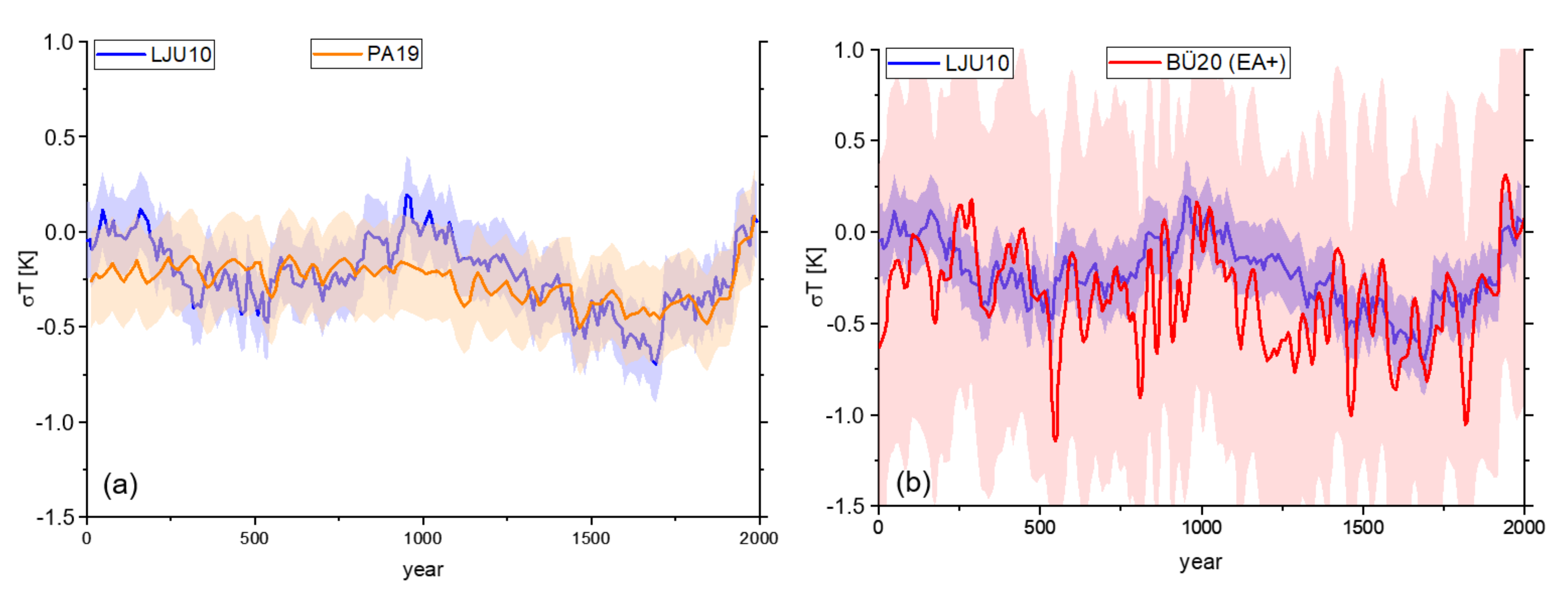
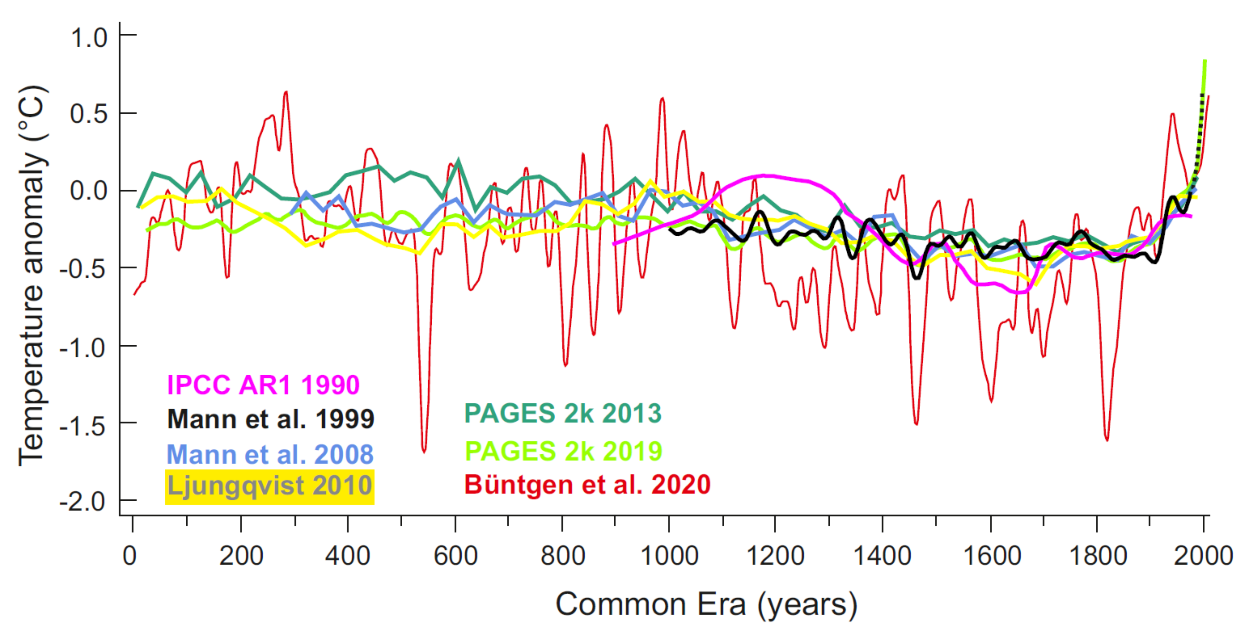
3. Comparison of Reconstructions

AR1 only shows a schematic temperature development in which a Medieval Warm Period (MWP, 1000–1300 CE) is illustrated that is clearly warmer than the subsequent Little Ice Age (LIA, 1400–1850 CE) (Figure 1 and Figure 2). The AR1 chart ends in 1990 but, from the overall geometry, it can be inferred that the MWP may have reached temperature levels similar to the current warm period (CWP) today. In the subsequent MM99 multi-proxy reconstruction, MWP and LIA differ very little, whilst the CWP is significantly warmer. Due to the shape of the curve, the reconstruction has also been termed “hockey stick” curve, which appeared prominently in the Summary for Policymakers in the IPCC AR3 report. Nearly ten years later, a group led by the same lead author updated the reconstruction (MM08), which contained a much larger temperature difference between MWP and LIA. The CWP was shown as warmer than the MWP.

Another two years later, LJU10 was published, which, again, showed a clear differentiation of the MWP and LIA that differed by nearly 1 °C. Warming levels of MWP and CWP were similar. Coverage was now extended to the past 2k and contained a warm “Roman Warm Period” (RWP, 1–200 CE) and a cold “Dark Ages Cold Period” (DACP, 300–800 CE). In PA13, the RWP remained warm, but part of the DACP was now warmer than the MWP and even warmer than the CWP. The LIA was shown as a pronounced cold phase. The same consortium produced a new reconstruction six years later (PA19) that fundamentally differed from their previous version (PA13), using seven different statistical methods. Their version, based on the method of “offline data assimilation“ (DA), shows a similar development as in MM99, i.e., returning to a “hockey stick” shape. Only a year later, BÜ20 published a tree-ring width reconstruction in which MWP and CWP reach similar maximum warming levels. The most extreme parts of the LIA are 2 °C colder than the warmest episodes of the MWP.

4. Discussion of Similarities and Possible Reasons for Discrepancies

There are some obvious similarities in all reconstructions, especially the characteristics of the Little Ice Age, which can be seen in all graphs. This is reassuring as already the IPCC AR1 report strongly pointed out that this has been a global phenomenon, clearly documented in historical records. MWP and LIA are considered the last two events of globally recognized Holocene rapid climate change [16]. Additionally, the variance in data, likely an intrinsic property of the multi-proxy reconstruction approach, confirms that, although the T curves appear quite different, their error intervals overlap such that they appear to not be in contradiction (see Supplementary Materials). Notably, there are some reconstructions that have markedly different features. For example, some versions do not show the details and amplitudes of alternating warm and cool periods, as, e.g., documented both in IPCC AR1 and LJU10 (Figure 2).

What might be the root cause of these discrepancies between the seven T2k reconstructions? It would be tempting to explain these mostly with differences in geographic coverage and proxy selection. However, this explanation is unlikely to hold true because even the “global” composites are dominated by sites from the Northern Hemisphere. Only a limited amount of data is available from the Southern Hemisphere. Higher-density Northern Hemisphere data can, of course, be the starting point of any robust reconstruction. It makes sense to begin in a well-documented region (e.g., Europe) and then expand to other regions of the same hemisphere. These restrictions already remove a lot of uncertainty. In a second step, as much data as possible from other parts of the world must be added. This is important to avoid regional bias in larger-scale T2k composites. For example, the original idea that the MWP may have been predominantly a “regional North Atlantic phenomenon” [17] can no longer be supported because warming associated with the MWP has, meanwhile, also been documented from many other regions of the world, e.g., China, South America, Africa, Oceania and Antarctica [18,19,20,21,22].

Careful selection and justification of the regional representation is, however, only the starting point. Further sources of error in T2k reconstructions are likely related to issues with data availability, selection and statistical processing. While, originally, very little high-quality data were available in the 1990s for AR1 or for MM99, this situation has changed. Over the past two decades, the field of paleoclimatology has matured and has delivered a large number of high-resolution case studies [23]. This puts high demands on the selection and processing of proxies.

In particular, the mixing of different proxy types can be a potential source of error and can cause signal dilution. Any inclusion must be carefully justified; the validation needs to be documented separately, in detail. Example: PA13 and PA19 used tree ring series from the French Maritime Alps even though tree ring specialists had previously cautioned that they are too complex to be used as overall temperature proxies [24,25].

In contrast, BÜ20 were more selective; they relied on one type of proxy (in this case, tree rings) and validated every tree ring data set individually. Their T2k composite differs greatly from the studies that use bulk tree ring input. In some cases, composites have erroneously included proxies that later turned out to reflect hydroclimate rather than temperature (examples discussed in 18,19).

In other cases, outlier studies have been selected in which the proxies exhibited an anomalous evolution that could not be reproduced in neighbouring sites (e.g., MWP data from Pyrenees and Alboran Sea in PA13) [26]. Outliers can have several reasons, e.g., a different local development, invalid or unstable temperature proxies, or sample contamination.

Age models of individual sites can be off by more than 100 years due to sparse and potentially misleading radiocarbon dates, as well as outdated calibration. Due to age model uncertainties, reconstructed pre-industrial warm and cold phases will always appear less intense compared to modern thermometer-measured data for which timing is certain. The radiocarbon-related time-shifts of climate anomalies in individual sites artificially flatten the climate anomalies in any composite. This makes the comparison of reconstructed and measured data complicated, requiring extreme caution when plotting the two data types in one diagram.

Another major challenge is the proper use of statistical methods for calculating the T2k composites. Depending on the method, the results can differ greatly from each other, either emphasizing or subduing pre-industrial climate variability [14]. Today, publication of the proxy data base and statistical code has become common practice (e.g., PA13, PA19), allowing transparent verification and discussion of workflows and results. Earlier studies (e.g., MM99) were less open with sharing of climate proxies and statistical methods, which, at the time, led to a controversial debate about the validity of the results [27,28,29].

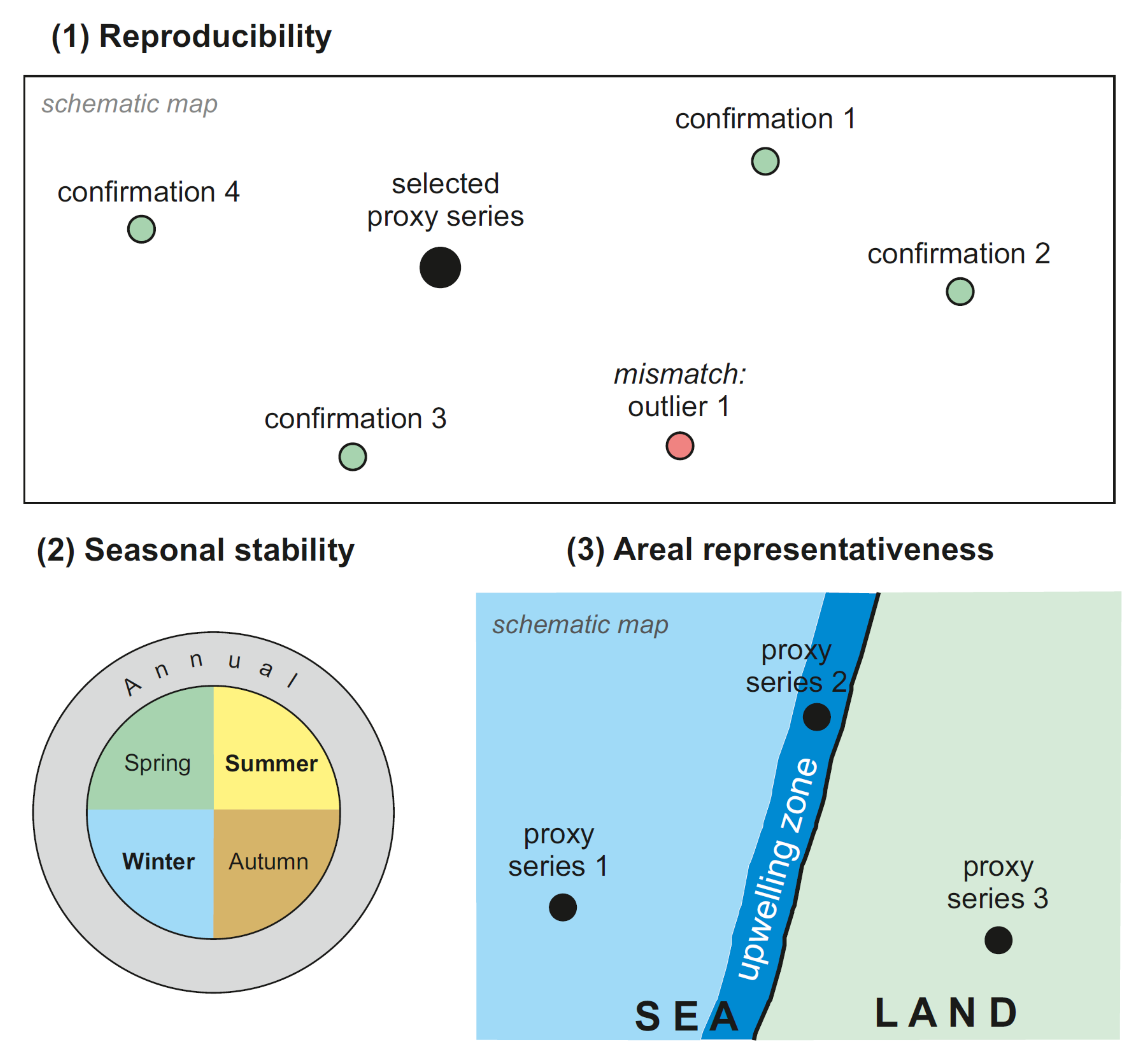
5. Criteria for Quality Assurance

We suggest the following approach to arrive at robust, consistent and reliable T2k composites. The first issue refers to attempted vs. real regional coverage. Rather than aiming at full hemisphere or even global temperature reconstructions, it may be more realistic to start with a robust reconstruction of a better documented region, e.g., central Europe or Alaska. Other important criteria that need to be considered when working with large proxy datasets are:

(1) Robust homogeneity/no outliers: The main climatic trends of each chosen proxy series need to be confirmed by at least two other sites from the same region, ideally using multiple methodologies. A data supplement should contain a thorough description and discussion of the respective sites, including a visual plot of the time series. Detailed integration with other results in the region is required, including studies that only provide qualitative data. The documentation will help to better identify outliers that must be eliminated prior to data stacking, as they would contaminate the composite.

(2) Seasonal stability: Temperature data need to be characterized as referring to annual, warm, or cold season to avoid seasonal bias. In case of major seasonal discrepancies, these are to be validated and reproduced in other sites in the region.

(3) Areal representativeness: The area for which a proxy series is considered representative needs to be clearly defined. Some sites only refer to small areas, such as narrow upwelling zones along some coastal stretches. There is a risk that such special regions are over-represented in continental and global composites. The greater abundance of data today, compared to two or three decades ago, now allows for a “paleoclimate mapping” approach so that spatial palaeoclimatic patterns can be considered. This includes the identification of characteristic weather and climate dipoles that also occur in the modern climate [30]. Areas without data need to be clearly identified and their infill method qualitatively justified based on the areal representativeness of nearby data. The selection of sites for T2k global composites need to be areally weighted according to the respective share of the continents in the global landmass. This helps to avoid over- and under-representation of regions in the composite. Marine and terrestrial sites, if mixed in composites, need to be thoroughly separated, as warm phases are typically more pronounced on land than in the seas. Mapping of palaeoclimate patterns in the oceans is particularly important, as temperature changes can also occur due to regional shifts in currents. A graphical representation of three criteria is shown in Figure 3.

6. Plausibility of Reconstructions

T2k composites should, preferably, be compiled independently by several academic groups to avoid monopolization and to achieve a healthy scientific competition that is so essential for the scientific process. PA13 consisted of 78 co-authors whose views may have partly differed—a rather difficult situation in such a large team. In addition, there seems to have been a certain preference of approaches: The 2000s were dominated by the conclusions of MM99 and MM08; the 2010s were mostly influenced by PA13 and P19. We believe that climate science would benefit from more diversification in the important field of T2k composites.

Given the large amount of potential error and arbitrary factors, any T2k regional reconstruction for a certain region must also be cross-checked with qualitative and semi-quantitative historical records. If there are any discrepancies between a T reconstruction and the historically documented climate periods, the burden of proof lies foremost with the composite reconstruction rather than with the historical data. Clearly, scientific or political conclusions can only be drawn on reliable, robust, and reproducible T reconstructions.

7. Conclusions

Due to its enormous significance for the attribution of modern climate change, a dedicated research program is needed to systematically fill the remaining large areas in the world for which high resolution and high quality T2k data is lacking. Doubtful outlier data that have been incorporated in previous T2k composites need to be double-checked with multiple methodologies to make the database as robust as possible. For reasons of simplification, we have discussed only seven T2k series in this contribution. Various other hemispheric to global temperature reconstructions exist, as well as related discussions (e.g., [31,32,33,34]). Lastly, T2k composites should be compiled independently by several academic groups to avoid monopolization and to achieve a healthy scientific discussion. PA13 consisted of 78 co-authors whose views may have partly differed, which, however, could not be expressed realistically due to the excessive team size. Whilst the 2000s were dominated by the view of MM99 and MM08, the 2010s were mostly influenced by LJU10 and PA13, and the early 2020s by PA19 (as prominently used in the IPCC’s 6th Assessment report, AR6). At the same time, BÜ20 was ignored in AR6 even though it was published before the literature cut-off data. Climate science would benefit from more diversification in the important field of T2k composites.

References

1. IPCC. First Assessment Report. 1990. Available online: http://www.ipcc.ch/publications_and_data/publications_and_data_reports.shtml (accessed on 30 January 2022).
2. Frank, D.; Esper, J.; Zorita, E.; Wilson, R. A noodle, hockey stick, and spaghetti plate: A perspective on high-resolution paleoclimatology. WIREs Clim. Chang. 2010, 1, 507–516. [Google Scholar] [CrossRef] [Green Version]
3. Christiansen, B.; Ljungqvist, F.C. Challenges and perspectives for large-scale temperature reconstructions of the past two millennia. Rev. Geophys. 2017, 55, 40–96. [Google Scholar] [CrossRef]
4. IPCC. Climate Change 2001: The Scientific Basis; Cambridge University Press: Cambridge, UK, 2001. [Google Scholar]
5. Mann, M.E.; Bradley, R.S.; Hughes, M.K. Northern Hemisphere Temperatures during the past Millennium: Inferences, Uncertainties, and Limitations. Geophys. Res. Lett. 1999, 26, 759–762. [Google Scholar] [CrossRef] [Green Version]
6. National Research Council. Surface Temperature Reconstructions for the Last 2000 Years; The National Academies Press: Washington, DC, USA, 2006. [Google Scholar]
7. Hegerl, G.; Zwiers, F. Use of models in detection and attribution of climate change. WIREs Clim. Chang. 2011, 2, 570–591. [Google Scholar] [CrossRef]
8. Smerdon, J.E. Climate models as a test bed for climate reconstruction methods: Pseudoproxy experiments. WIREs Clim. Chang. 2012, 3, 63–77. [Google Scholar] [CrossRef] [Green Version]
9. Smerdon, J.E.; Pollack, H.N. Reconstructing Earth’s surface temperature over the past 2000 years: The science behind the headlines. WIREs Clim. Chang. 2016, 7, 746–771. [Google Scholar] [CrossRef]
10. Folland, C.K.; Karl, T.R.; Vinnikov, K.Y. Observed Climate Variations and Change. In Climate Change: The IPCC Scientific Assessment; 1st Assessment Report (AR1); Houghton, J.T., Jenkins, G.J., Ephraums, J.J., Eds.; Cambridge University Press: Cambridge, UK, 1990; Chapter 7; p. 202. [Google Scholar]
11. Mann, M.E.; Zhang, Z.; Hughes, M.K.; Bradley, R.S.; Miller, S.K.; Rutherford, S.; Ni, F. Proxy-based reconstructions of hemispheric and global surface temperature variations over the past two millennia. Proc. Natl. Acad. Sci. USA 2008, 105, 13252–13257. [Google Scholar] [CrossRef] [PubMed] [Green Version]
12. Ljungqvist, F.C. A new reconstruction of temperature variability in the extra-tropical northern hemisphere during the last two millennia. Geogr. Ann. Ser. A 2010, 92, 339–351. [Google Scholar] [CrossRef]
13. PAGES 2k Consortium. Continental-scale temperature variability during the past two millennia. Nat. Geosci. 2013, 6, 339–346. [Google Scholar] [CrossRef]
14. PAGES 2k Consortium. Consistent multidecadal variability in global temperature reconstructions and simulations over the Common Era. Nat. Geosci. 2019, 12, 643–649. [Google Scholar] [CrossRef] [Green Version]
15. Büntgen, U.; Arseneault, D.; Boucher, É.; Churakova, O.V.; Gennaretti, F.; Crivellaro, A.; Hughes, M.K.; Kirdyanov, A.V.; Klippel, L.; Krusic, P.J.; et al. Prominent role of volcanism in Common Era climate variability and human history. Dendrochronologia 2020, 64, 125757. [Google Scholar] [CrossRef]
16. Mayewski, P.A.; Rohling, E.E.; Stager, J.C.; Karlén, W.; Maasch, K.A.; Meeker, L.D.; Meyerson, E.A.; Gasse, F.; van Kreveld, S.; Holmgren, K.; et al. Holocene climate variability. Quat. Res. 2004, 62, 243–255. [Google Scholar] [CrossRef]
17. Mann, M.E.; Zhang, Z.; Rutherford, S.; Bradley, R.S.; Hughes, M.K.; Shindell, D.; Ammann, C.; Faluvegi, G.; Ni, F. Global Signatures and Dynamical Origins of the Little Ice Age and Medieval Climate Anomaly. Science 2009, 326, 1256–1260. [Google Scholar] [CrossRef] [PubMed] [Green Version]
18. Lüning, S.; Gałka, M.; Bamonte, F.P.; Rodríguez, F.G.; Vahrenholt, F. The Medieval Climate Anomaly in South America. Quat. Int. 2019, 508, 70–87. [Google Scholar] [CrossRef]
19. Lüning, S.; Gałka, M.; Vahrenholt, F. Warming and Cooling: The Medieval Climate Anomaly in Africa and Arabia. Paleoceanography 2017, 32, 1219–1235. [Google Scholar] [CrossRef]
20. Lüning, S.; Gałka, M.; García-Rodríguez, F.; Vahrenholt, F. The Medieval Climate Anomaly in Oceania. Environ. Rev. 2020, 28, 45–54. [Google Scholar] [CrossRef]
21. Lüning, S.; Gałka, M.; Vahrenholt, F. The Medieval Climate Anomaly in Antarctica. Palaeogeogr. Palaeoclimatol. Palaeoecol. 2019, 532, 109251. [Google Scholar] [CrossRef]
22. Hao, Z.; Wu, M.; Liu, Y.; Zhang, X.; Zheng, J. Multi-scale temperature variations and their regional differences in China during the Medieval Climate Anomaly. J. Geogr. Sci. 2020, 30, 119–130. [Google Scholar] [CrossRef] [Green Version]
23. Lüning, S. Google Map of publications on the Medieval Climate Anomaly. 2021. Available online: http://t1p.de/mwp (accessed on 30 January 2022).
24. Seim, A.; Büntgen, U.; Fonti, P.; Haska, H.; Herzig, F.; Tegel, W.; Trouet, V.; Treydte, K. Climate sensitivity of a millennium-long pine chronology from Albania. Clim. Res. 2012, 51, 217–228. [Google Scholar] [CrossRef]
25. Büntgen, U.; Frank, D.; Neuenschwander, T.; Esper, J. Fading temperature sensitivity of Alpine tree growth at its Mediterranean margin and associated effects on large-scale climate reconstructions. Clim. Chang. 2012, 114, 651–666. [Google Scholar] [CrossRef] [Green Version]
26. Lüning, S.; Schulte, L.; Garcés-Pastor, S.; Danladi, I.B.; Gałka, M. The Medieval Climate Anomaly in the Mediterranean Region. Paleoceanogr. Paleoclimatol. 2019, 34, 1625–1649. [Google Scholar] [CrossRef]
27. McShane, B.B.; Wyner, A.J. A statistical analysis of multiple temperature proxies: Are reconstructions of surface temperatures over the last 1000 years reliable? Ann. Appl. Stat. 2011, 5, 5–44. [Google Scholar]
28. McShane, B.B.; Wyner, A.J. Rejoinder. Ann. Appl. Stat. 2011, 5, 99–123. [Google Scholar] [CrossRef]
29. McIntyre, S.; McKitrick, R. Corrections to the Mann et al. (1988) proxy data base and northern hemispheric average temperature series. Energy Environ. 2003, 14, 751–771. [Google Scholar] [CrossRef]
30. Zuckerberg, B.; Strong, C.; LaMontagne, J.M.; George, S.S.; Betancourt, J.L.; Koenig, W.D. Climate Dipoles as Continental Drivers of Plant and Animal Populations. Trends Ecol. Evol. 2020, 35, 440–453. [Google Scholar] [CrossRef] [PubMed]
31. Connolly, R.; Connolly, M. Global temperature changes of the last millennium. Open Peer Rev. J. 2014, 2014, 16. [Google Scholar]
32. Wilson, R.; Anchukaitis, K.; Briffa, K.R.; Büntgen, U.; Cook, E.; D’Arrigo, R.; Davi, N.; Esper, J.; Frank, D.; Gunnarson, B.; et al. Last millennium northern hemisphere summer temperatures from tree rings: Part I: The long term context. Quat. Sci. Rev. 2016, 134, 1–18. [Google Scholar] [CrossRef] [Green Version]
33. Xing, P.; Chen, X.; Luo, Y.; Nie, S.; Zhao, Z.; Huang, J.; Wang, S. The Extratropical Northern Hemisphere Temperature Reconstruction during the Last Millennium Based on a Novel Method. PLoS ONE 2016, 11, e0146776. [Google Scholar] [CrossRef] [Green Version]
34. Schneider, L.; Smerdon, J.E.; Büntgen, U.; Wilson, R.J.S.; Myglan, V.S.; Kirdyanov, A.V.; Esper, J. Revising midlatitude summer temperatures back to A.D. 600 based on a wood density network. Geophys. Res. Lett. 2015, 42, 4556–4562. [Google Scholar] [CrossRef] [Green Version]
Figure 1. Comparison of the seven T2k composites. Anomaly refers to 1961–1990 temperature average. Smoothing filters: 40 years for MM99 and MM08, 30 years for LJU10, PA13, PA19, and BÜ20.
Earth 03 00024 g001
Figure 2. Comparison of reconstruction LJU10 vs. PA19 (a), and LJU10 vs. BÜ20 (b), including error bars. The temperature measurements contained in the original manuscript are not displayed.
Earth 03 00024 g002
Figure 3. Quality criteria for palaeotemperature proxy selection (see text for details).
Earth 03 00024 g003