A New Model of Solar Illumination of Earth’s Atmosphere during Night-Time

Abstract

In this work, a solar illumination model of the Earth’s atmosphere is developed. The developed model allows us to determine with extreme accuracy how the atmospheric illumination varies during night hours on a global scale. This time-dependent variation in illumination causes a series of sudden changes in the entire Earth-atmosphere-ionosphere system of considerable interest for various research sectors and applications related to climate change, ionospheric disturbances, navigation and global positioning systems. The use of the proposed solar illumination model to calculate the time-dependent Solar Terminator Height (STH) at the global scale is also presented.Time-dependent STH impact on the measurements of ionospheric Total Electron Content (TEC) is, for the first time, investigated on the basis of 20 years long time series of GPS-based measurements collected at ground. The correlation analysis, performed in the post-sunset hours, allows new insights into the dependence of TEC–STH relation on the different periods (seasons) of observation and solar activity conditions.

1. Introduction

The dividing boundary between the day and night side of the Earth and its atmosphere is called Solar Terminator (ST). Its position on the ground determines the times of sunrise and sunset. Solar illumination reaching the two sides of this region differently contributes to the energy balance at different heights in the atmosphere. Such a differential, time-dependent, illumination generates sudden changes throughout the whole Earth-atmosphere-ionosphere system. Among the consequences of such a vertical (and horizontal) ST variation during the time there are: generation of acoustic gravity waves (AGW) [1,2,3,4,5,6] which, manifesting themselves at ionospheric heights as traveling ionospheric disturbances (TID), are responsible for the transport of energy and momentum in the near-Earth space; oscillations of vertical pressure and temperature gradients as well as of neutral and ionic atmospheric components (such as N2, O, O+, NO+, O2+) of particular interest for the study of climate change [7]; significant effects on wave propagation of all frequencies (ULF, VLF, LF, HF, etc.) [8] and on Total Electron Content [9], both of considerable interest for their significant influence on radio transmissions and for the study of the ionospheric effects of seismic activity. Moreover, as demonstrated by [10], over the equatorial region, horizontal and vertical components of AGW phase velocity coincide with horizontal and vertical components of the terminator velocity. For example, in the study of atmospheric gravitational waves, it is important to accurately determine the time, latitudes and altitudes in which the speed of variation of terminator becomes supersonic because in this space–time interval it can generate gravitational waves [1].

Vertical movements of the ST are particularly relevant for the construction of ionospheric empirical models [11]. They affect the composition and transport dynamics of plasma (temperature and ion/electron concentration) providing basic information required to separate day and night conditions at different ionospheric layers. On this basis, in fact, it is possible to predict the layer D disappearance during the night or the elevation changes of the F2 layer peak. Similarly, the knowledge of ST movements is fundamental for the interpretation of the differential illumination of lower ionospheric layers that can oscillate following the regular alternation of day and night while, in certain conditions (e.g., at high latitudes), the upper layers remain always irradiated.

Despite its multi-disciplinary importance, a detailed model for the determination of ST vertical movements is still lacking. In the scientific literature available to date, manuscripts dealing with the subject [12] provide only partial solution equations.

In this paper, a Solar Terminator Height (STH) model is proposed which provides, with unprecedented accuracy and at the global scale, the vertical variation of the ST as a function of time.

The model also offers methodological support and solution equations to go beyond a series of approximations (e.g., use of the spherical shape of the Earth, not precise Earth–Sun position, use of sidereal time, use of the mean terrestrial radius, etc.) still used in all field of applications, even when greater accuracy would improve the performances.

As an example of the impact of ST variations on space–time dynamics of atmospheric parameters, the case of ionospheric Total Electron Content (TEC) is particularly addressed.

The TEC represents the number of electrons present along a ray path of 1 m² of an ionospheric section, measured in TEC Unit (1 TEC Unit = 10¹⁶ electrons/m²), and can be determined by ground-based (e.g., from ionosondes, Global Navigation Satellite Systems receivers [13]) and space-based (e.g., FORMOSAT/COSMIC series [14,15], DEMETER [16]) measurements.

In this work, a statistically-based analysis of 20 years of GPS (Global Positioning System)-TEC data measured over Central Italy during the period 2000–2019 is performed in order to recognize its dependence on STH space–time variations.

The analysis here implemented investigates, for the first time, the correlations between TEC measurements and STH. In the post-sunset hours, in fact, the sudden variation in solar irradiation incident on the various ionospheric layers generates variation in total ionization. Such a study can be particularly useful in the elaboration of ionospheric TEC models as well as in those applications requiring predicting the behavior of TEC parameter in specific conditions.

Moreover, due to the fact that the ionosphere directly influences trans-ionospheric radio waves propagating from satellites to GNSS receivers [17,18], such models are of vital importance in order to evaluate and correct errors (that can be quite significant) in GNSS-positioning due to TEC ionospheric irregularities. No less important is the role that TEC models play in the study of the possible relations between ionospheric perturbations and seismic activity, theorized by several authors in recent years [19,20,21,22,23].

2. Materials and Methods

This section is divided into two subsections. In the first one, we illustrate the proposed time-dependent STH model describing how the atmospheric solar illumination varies during the night along the vertical at a given geographical position. In the second, we report the method used for the statistical correlation analysis between STH and the ionospheric TEC parameter measured over Central Italy.

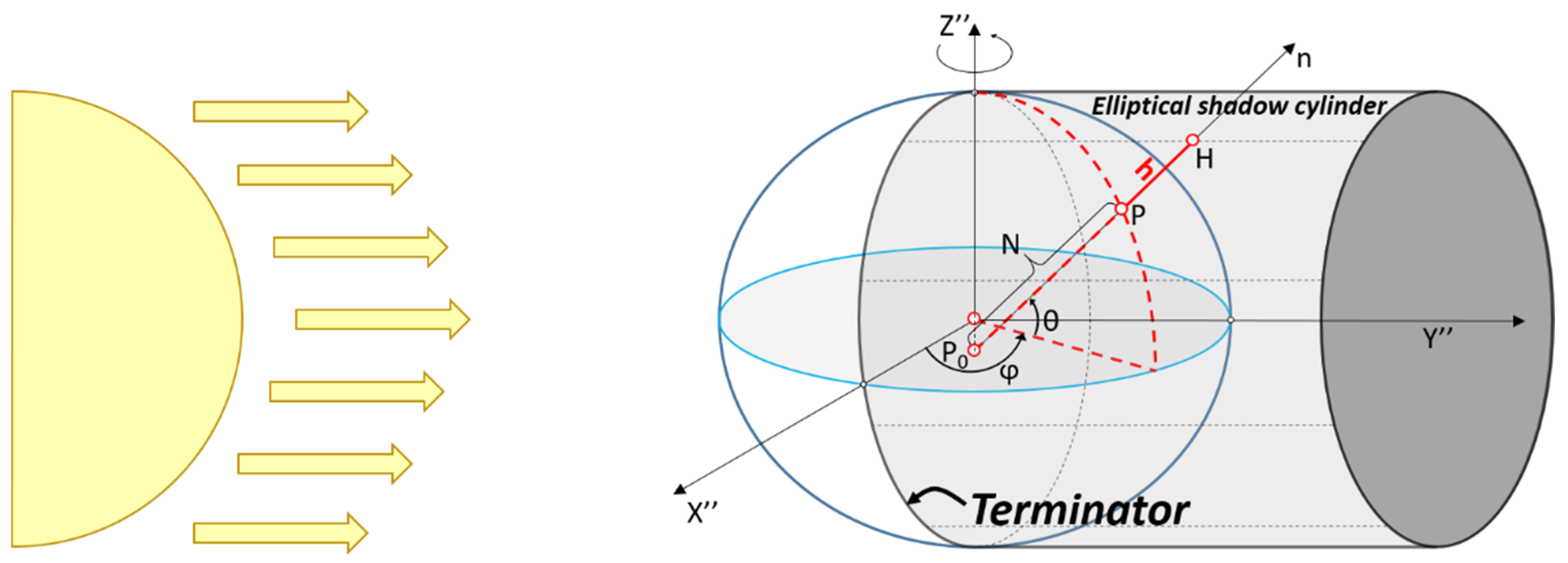
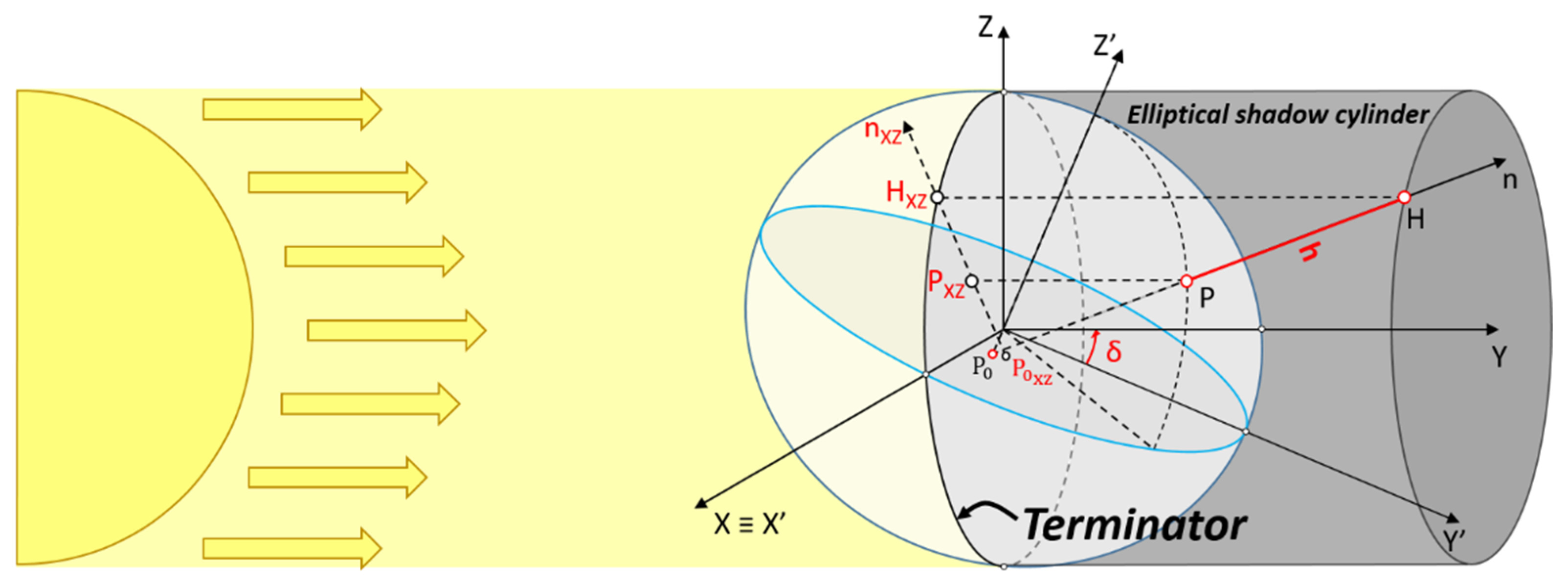
2.1. Solar Terminator Height Determination

The Solar Terminator Height (STH) at time t, h (θ, φ, t) for a given point P, at latitude θ and longitude φ on the Earth’s surface, represents the height of the Sun-shadow demarcation line (solar terminator) at the instant t along the vertical at point P (θ, φ).

The only assumptions we make in the mathematical modelling are: solar rays parallel to each other and ellipsoidal (WGS84) shape of the Earth.

The vertical height of the point P above the Earth’s surface is a line joining the point P and a point H along the local ellipsoid’s normal n (Figure 1). The length $\overline{PH}$ is called the ellipsoidal height h. The ellipsoid’s normal n is a straight line perpendicular to the plane tangent to the ellipsoid at the point P and which, then, crosses in a generic point P₀ the axis of rotation of the Earth.

Therefore, the terminal point H (θ, φ, t) of the solar terminator ellipsoidal height h (θ, φ, t) is given by the intersection between n and the boundary of the shape generated by the shadow produced by the Earth’s ellipsoid illuminated by the Sun’s rays (elliptical shadow cylinder shown in Figure 1).

By choosing WGS84 as reference ellipsoid and by choosing a Cartesian reference system, which for convenience we call X″Y″Z″, having the Z″ axis coinciding with the Earth’s rotation axis, the X″Y″ plane coinciding with the equatorial plane and the X″ axis which intersects the prime meridian on the positive side (Figure 1), it is possible to determine the ellipsoidal height h by making it explicit from any of the well-known conversion formulas provided by geodesy:

$${X^{″}}_H=\left(N+h\right)·\cos \theta ·\cos \phi ;$$

(1)

$${Y^{″}}_H=\left(N+h\right)·\cos \theta ·\sin \phi ;$$

(2)

$${Z^{″}}_H=\left[N·\left(1-e^2\right)+h\right]·\sin \theta ;$$

(3)

where:

• H is the terminal point of the ellipsoidal height h;
• $N=\frac{a}{\sqrt{1-e^2·si{n}^2\theta }}$ is the length of the straight line coinciding with the ellipsoid’s normal n connecting the point P and the point of intersection between n and Z″ axis P₀ (length $\overline{P{P}_0}$ in Figure 1);
• e² and a, respectively equal to 0.00669438 and to 6,378,137 m, are the ellipsoidal parameters first eccentricity squared and semi-major axis of the reference ellipsoid used (WGS84);
• θ and φ are, respectively, the geodetic latitude and the longitude.

Since we are interested in determining the variation of h as a function of time (and therefore of the angle of rotation of the Earth around its axis), for our purposes it is more convenient to choose a new X′Y′Z′ reference system, rotating the X″Y″Z″ system around the Z″ axis, so that, as the Earth rotates, our reference system rotates in the opposite direction, making sure that the positive side of the X′ axis always passes through the point of intersection between sunset line and equatorial plane (Figure 1 shows the moment of the day in which X′Y′Z′ coincides with X″Y″Z″).

In order for the proposed equations, (1), (2) and (3), to be valid in the new X′Y′Z′ reference system, we replace the longitude φ with the angle measured on the equatorial plane between the meridian passing through the X′ axis (sunset line) and the meridian passing through the point P. We call this angle λ, local hour angle from sunset. λ, which varies according to the Earth’s rotation, will subsequently be accurately determined.

In the new reference system X′Y′Z′, we have:

$${X^{\prime }}_H=\left(N+h\right)·\cos \theta ·\cos \lambda ;$$

(4)

$${Y^{\prime }}_H=\left(N+h\right)·\cos \theta ·\sin \lambda ;$$

(5)

$${Z^{\prime }}_H=\left[N·\left(1-e^2\right)+h\right]·\sin \theta ;$$

(6)

with λ = local hour angle from sunset.

Furthermore, due to the revolution motion of the Earth around the Sun, the equatorial plane tilts with respect to the direction of the Sun’s rays by an angle δ (solar declination). δ reaches a maximum angle in June at the moment of the Northern Hemisphere summer solstice, which is about 23.44°, and a minimum angle in December at the moment of the Northern Hemisphere winter solstice, which is about −23.44°. Since the X′ axis is perpendicular to the direction of the Sun’s rays, the rotation of the angle δ takes place around the X′ axis itself. Thus, we define a new reference system XYZ obtained by rotating the X′Y′Z′ reference system by the angle -δ around the X′ axis (see Figure 2). The angle δ will be calculated later.

In the XYZ system, we have:

$$X_H=X_H^{\prime }=\left(N+h\right)·\cos \theta ·\cos \lambda ;$$

(7)

$$\begin{array}{c}{Y}_H=Y_H^{\prime }·\cos \delta -Z_H^{\prime }·\sin \delta =\\ =\left(N+h\right)·\cos \theta ·\sin \lambda ·\cos \delta -\left[N·\left(1-e^2\right)+h\right]·\sin \theta ·\sin \delta ;\end{array}$$

(8)

$$\begin{array}{c}{Z}_H=Y_H^{\prime }·\sin \delta -Z_H^{\prime }·\cos \delta =\\ =\left(N+h\right)·\cos \theta ·\sin \lambda ·\sin \delta -\left[N·\left(1-e^2\right)+h\right]·\sin \theta ·\cos \delta .\end{array}$$

(9)

Solving Equation (7) for h gives:

$$h=\frac{X_H}{\cos \theta ·\cos \lambda }-N;if:\alpha \le 0°$$

(10)

where α = solar elevation angle, to be defined later.

Therefore, we need to calculate X_H to determine h. To do this, it is possible to exploit the fact that (given the assumption of solar rays all parallel to each other) the projection on the XZ plane of the point H is a point H_xz given by the intersection between the projection on the XZ plane of n (n_xz) and the ellipsoid E (see Figure 2). It will, then, be necessary to determine the equation of the two geometric figures (n and E) and their intersection at the point H_xz.

n_xz is a straight line passing through the projections on the XZ plane of the points P and P₀. The coordinates of the points P and P₀ in the X″Y″Z″ reference system are given, again, by the well-known equations of the ellipsoid’s normal provided by geodesy:

$${X^{″}}_P=N·\cos \theta ·\cos \phi ;$$

(11)

$${Y^{″}}_P=N·\cos \theta ·\sin \phi ;$$

(12)

$${Z^{″}}_P=N·\left(1-e^2\right)·\sin \theta ;$$

(13)

$$X_{P_0}^{{}^{″}}=0;$$

(14)

$$Y_{P_0}^{{}^{″}}=0;$$

(15)

$$Z_{P_0}^{{}^{″}}=-e^2·N·\sin \theta .$$

(16)

Applying the equations of rotation already used to rotate the point H from the reference system X″Y″Z″ to the reference system XYZ, the points P and P₀ in XYZ are given by the following expressions:

$$X_P=N·\cos \theta ·\cos \lambda ;$$

(17)

$$Z_P=N·\cos \theta ·\sin \lambda ·\sin \delta +N·\left(1-e^2\right)·\sin \theta ·\cos \delta ;$$

(18)

$$X_{P_0}=0;$$

(19)

$$Z_{P_0}=-e^2·N·\sin \theta ·\cos \delta .$$

(20)

At this point, we can determine the equation of the line n_xz passing through the points P e P₀ (and through the point H_xz; see Figure 2):

$$\frac{X_n-X_{P_0}}{X_P-X_{P_0}}=\frac{Z_n-Z_{P_0}}{Z_P-Z_{P_0}};$$

(21)

$$X_n=\frac{Z_n-Z_{P_0}}{Z_P-Z_{P_0}}·X_P.$$

(22)

From the Equations (17), (18) and (20), after some simplifications, we have:

$$\frac{X_P}{Z_P-Z_{P_0}}=\frac{\cos \lambda }{\sin \lambda ·\sin \delta +\tan \theta ·\cos \delta };$$

(23)

defining:

$$C_1=\frac{\cos \lambda }{\sin \lambda ·\sin \delta +\tan \theta ·\cos \delta };$$

(24)

we can write:

$$X_n=\left(Z_n-Z_{P_0}\right)·C_1.$$

(25)

Let’s now move on to the equation of the ellipsoid E, which, in the X″Y″Z″ reference system, coincides with the one in the X′Y′Z′ reference system:

$$\frac{{X^{\prime }}_E{}^2+{Y^{\prime }}_E{}^2}{a^2}+\frac{{Z^{\prime }}_E{}^2}{c^2}=1;$$

(26)

where c, equal to 6,356,752.314 m, is the semi-minor ellipsoid parameter of the reference ellipsoid used (WGS84).

We determine the equation of the coordinate X_E as a function of Z_E on the XZ plane (for Y = 0). Again exploiting the rotation equations of the reference system, in XYZ, after some substitutions, we have:

$$X_E^{\prime }=X_E;$$

(27)

$$Y_E^{\prime }=Z_E^{\prime }·\frac{\sin \delta }{\cos \delta }=Z_E^{\prime }·\tan \delta ;$$

(28)

$$Z_E^{\prime }=\frac{Z_E-Y_E^{\prime }·\sin \delta }{\cos \delta }=\frac{Z_E-Z_E^{\prime }·\tan \delta ·\sin \delta }{\cos \delta }=\frac{Z_E}{\cos \delta }-Z_E^{\prime }·{\tan }^2\delta ;$$

(29)

from which:

$$Z_E^{\prime }=\frac{Z_E}{\cos \delta ·\left(1+{\tan }^2\delta \right)};$$

(30)

$$Y_E^{\prime }=\frac{Z_E·\tan \delta }{\cos \delta ·\left(1+{\tan }^2\delta \right)}.$$

(31)

By replacing Equations (27), (31) and (30) in (26), we have:

$$\frac{X_E^2}{a^2}+{\left[\frac{Z_E·\tan \delta }{a·\cos \delta ·(1+{\tan }^2\delta )}\right]}^2+{\left[\frac{Z_E}{c·\cos \delta ·(1+{\tan }^2\delta )}\right]}^2=1;$$

(32)

$$\frac{X_E^2}{a^2}+{\left[\frac{Z_E·\tan \delta }{a·\cos \delta ·(1+{\tan }^2\delta )}\right]}^2+{\left[\frac{Z_E}{c·\cos \delta ·(1+{\tan }^2\delta )}\right]}^2=1;$$

(33)

$$\frac{X_E^2}{a^2}+Z_E^2·\frac{1}{{\left[\cos \delta ·(1+{\tan }^2\delta )\right]}^2}·\left(\frac{{\tan }^2\delta }{a^2}+\frac{1}{c^2}\right)=1;$$

(34)

$$X_E^2=a^2-Z_E^2·\frac{1}{{\left[\cos \delta ·(1+{\tan }^2\delta )\right]}^2}·\left({\tan }^2\delta +\frac{a^2}{c^2}\right).$$

(35)

Defining:

$$C_2=\frac{1}{{\left[\cos \delta ·(1+{\tan }^2\delta )\right]}^2}·\left({\tan }^2\delta +\frac{a^2}{c^2}\right);$$

(36)

we can write:

$$X_E^2=a^2-Z_E^2·C_2;$$

(37)

and, squaring the Equation (25), we obtain:

$$X_n^2=Z_n^2·C_1^2-Z_n·\left(2·Z_{P_0}·C_1^2\right)+Z_{P_0}^2·C_1^2.$$

(38)

Thus, given the expressions of X_n (Z_n) and X_E (Z_E), (38) and (37), it is possible to determine their point of intersection Z_H (X_H) by equating them:

$$Z_H^2·\left(C_1^2+C_2\right)-Z_H·\left(2·Z_{P_0}·C_1^2\right)+Z_{P_0}^2·C_1^2-a^2=0.$$

(39)

Defining:

$$K_1=C_1^2+C_2;$$

(40)

$$K_2=2·Z_{P_0}·C_1^2;$$

(41)

$$K_3=Z_{P_0}^2·C_1^2-a^2;$$

(42)

we can write:

$$Z_H{}_{}=\frac{K_2\pm \sqrt{K_2^2-4·K_1·K_3}}{2K_1}.$$

(43)

We use the positive sign if θ + δ > 0 and the negative sign if θ + δ < 0.

From Equation (25), it follows that:

$$X_H=\left(Z_H-Z_{P_0}\right)·C_1;$$

(44)

and, finally, it is possible to compute the Equation (10):

$$h=STH=\frac{X_H}{\cos \theta ·\cos \lambda }-N.if:\alpha \le 0°$$

(45)

The last step consists in determining the three unknown angles:

• Solar declination angle δ;
• Local hour angle from sunset λ;
• Solar elevation angle α.

We use the equations proposed in Chapters 25, 7, 22 and 30 of the book Astronomical Algorithms [24] for the accurate determination of the solar declination angle δ and the equations proposed in Chapters 28, 22 and 25 of the same book [24] for the determination of the equation of time ET, as a function of which the angles λ and α will then be determined. The proposed equations can also be deduced from the spreadsheets available online on the NOAA solar calculator website [25], also based on the book Astronomical Algorithms [24]. However, given that the equations proposed by [24] have different scopes from those proposed in the present work and different possibilities of choosing the “previous parameters” according to the use of the “dependent parameters” and that over time there have been some updates to the equations, it is preferred to reorganize them and report them below for clarity and simplicity of use.

2.1.1. Solar Declination Angle: δ

The equations proposed in Chapters 25, 7, 22 and 30 of [24] for the accurate determination of the solar declination angle δ are then reorganized below.

Defining JD as the Julian Day from the epoch “1 January 2000 12:00:00 UTC”, it is possible to determine the time T expressed in Julian centuries:

$$T=\frac{JD}{36525};$$

(46)

It is considered superfluous to report the JD calculation procedure as nowadays any programming language has at least one function for its calculation; in any case, the procedure can be found in Chapter 7 of [24].

Thus, the Sun’s Mean Longitude (ML), referring to the mean equinox of the date (decimal degrees), is:

$$ML=280.46646°+\mathrm{T}\left(36000.76983°+0.0003032°·\mathrm{T}\right);$$

(47)

where 280.46646° is the mean longitude of the Sun on 1 January 2000 at noon UTC (mean equinox of the date).

Then, the Sun’s Mean Anomaly MA is given by:

$$MA=357.52911°+\mathrm{T}\left(35999.05029°-0.0001537°·\mathrm{T}\right);$$

(48)

MA is defined as “the angular distance from perihelion which the planet would have if it moved around the Sun with a constant angular velocity” [24] (Cap. 30, p. 194).

As a function of MA, it is now possible to calculate the Sun’s equation of the center C, that is, the angular difference between the actual position of a body in its elliptical orbit and the position it would occupy if its motion were uniform in a circular orbit of the same period.

C can be performed as follows:

$$\begin{gathered} C=\sin \left(MA\right)·\left(1.914602°-T\left(0.004817°+0.000014°·T\right)\right) \\ +\sin \left(2T\right)·\left(0.019993°-0.000101°·T\right)+\sin \left(3T\right)·0.000289°; \end{gathered}$$

(49)

By adding Sun’s equation of the center C to Sun’s Mean Anomaly MA, we calculate the Sun’s true longitude TL (the true geometric longitude referred to the mean equinox of the date):

$$TL=ML+C;$$

(50)

The Sun’s Apparent longitude AL, i.e., TL corrected for the nutation and the aberration, is given by:

$$AL=TL-0.00569°-0.00478°·\sin (125.04°-1934.136°·T);$$

(51)

The next step is to calculate the mean obliquity of the ecliptic MOE. The equation proposed by the 1998 version of Astronomical Algorithms [24], which we are using as the main reference, shows terms up to the third order. This equation is still in use also in the spreadsheets available online on the NOAA solar calculator website [25], but the JPL’s fundamental ephemerides are constantly updated. In particular, the MOE calculation was updated in the Astronomical Almanac for the year 2010 [26], which, in addition to correcting the coefficients for the terms up to the third order, adds the terms of the fourth and fifth orders:

$$\begin{gathered} MOE=23°26{}^{\prime }21{}^{″},406-46{}^{″},836769T-0{}^{″}{,0001831T}^2+0{}^{″},00200340T^3 \\ -0{}^{″},576·{10}^{-6}{T}^4-4{}^{″},34·{10}^{-8}{T}^5; \end{gathered}$$

(52)

where, again, T is the time measured in Julian centuries from noon 1 January 2000 UTC.

Once MOE is known, it is possible to compute the obliquity corrected OC, which should be considered in order to calculate the apparent position of the Sun (position of the Sun corrected for the nutation and the aberration):

$$OC=MOE+0.00256°·\cos (125.04°-1934.136°·T);$$

(53)

Finally, the Sun’s declination δ is given by:

$$\delta =asin\left(\sin OC·\sin AL\right);$$

(54)

2.1.2. Equation of Time: ET (min)

For the precise determination of the angles λ and α, instead, we use the equation of time ET, the calculation of which is proposed in Chapter 28 (with references to Chapters 22 and 25) of the book Astronomical Algorithms [24].

ET is a corrective parameter of the heliocentric longitude of the Earth and therefore of solar time. In particular, it transforms the mean solar time MST into the true solar time TST.

MST, in fact, is calculated on the basis of the assumption of Earth’s constant velocity of revolution along a circular orbit, rather than an elliptical one. Furthermore, at a much lower magnitude, the equation of time also corrects the variations in the Earth’s speed along the elliptical due to the interaction with the Moon and with the planets.

ET expressed in minutes is given by the following expression:

$$\begin{gathered} ET=\left[y·\sin \left(2·ML\right)-2·e·\sin (MA)+4·e·y·\sin \left(MA\right)·\cos \left(2·ML\right) \\ -\raisebox{1ex}{$1$}\!\left/ \!\raisebox{-1ex}{$2$}\right.·y^2·\sin \left(4·ML\right)-\raisebox{1ex}{$5$}\!\left/ \!\raisebox{-1ex}{$4$}\right.e^2·\sin \left(2·MA\right)\right]·\frac{1440min}{360°}; \end{gathered}$$

(55)

where e = eccentricity of the Earth’s orbit:

$$e=0.016708634-0.000042037·T-0.0000001267·T^2;$$

(56)

y = coefficient of correction of the position of the Sun for the nutation and the aberration:

$$y={tan}^2\frac{OC}{2};$$

(57)

2.1.3. Local Hour Angle from Sunset λ

The angle λ is defined as the local hour angle from sunset since it represents the local hour angle LHA reduced by 90°. In fact, LHA, which is the angle between the meridian passing through the geographical position of the Sun and the meridian passing through the geographical position of the point P, measures 0° when the point P is at solar noon. Similarly, λ is equal to 0 when the meridian passing through the point P coincides with the meridian passing through the point where sunset occurs on the equatorial plane.

For its determination, the following 4 steps are carried out:

• HD (min/UTC), the hour of the day hh:mm:ss UTC of point P expressed in minutes, is calculated:

$$HD=hh·60+mm+\raisebox{1ex}{$ss$}\!\left/ \!\raisebox{-1ex}{$60$}\right.;$$

(58)

2.

TST (min/UTC), the true solar time of point P expressed in minutes, is obtained as follows:

$$TST=\left(HD+ET+4·\phi \right)mod1440min;$$

(59)

3.

LHA (°), the local hour angle of point P expressed in degrees, is given by:

$$LHA=\raisebox{1ex}{$TST$}\!\left/ \!\raisebox{-1ex}{$4$}\right.-180°;$$

(60)

4.

λ (°), local hour angle from sunset expressed in degrees, then, is:

$$\lambda =\left(LHA-90°\right)mod360°;$$

(61)

2.1.4. Solar Elevation Angle α

Finally, still exploiting the knowledge of the LHA, it is possible to calculate α (°), the solar elevation angle, expressed in degrees:

$$\alpha =asin\left(\sin \theta ·\sin \delta +\cos \theta ·\cos \delta ·\cos LHA\right).$$

(62)

A computer code for the time-dependent STH calculation for any geographic location on the globe was written using the R programming language [27]. This code can be found in the Supplementary Materials (Supplementary 1) to this paper.

2.2. STH–TEC Correlation Analysis

A simple look at the typical behavior of TEC measurements clearly enhances their strict dependence on the daily solar variation (see Figure 3, [28]).

Solar forcing also causes seasonal variations [29,30,31]; however, it is not the unique cause of ionospheric TEC deviations. For instance, geomagnetic activity (and storms) can significantly affect TEC so that, in order to discriminate solar from other contributions, it is particularly important to study those parts of the day (before sunrise or after sunset) when ionospheric layers are selectively illuminated by the Sun [32] (Figure 3).

In order to evaluate solar contribution to TEC variations (as a function of the specific location and time of year and in different conditions of solar activity), a correlation analysis with STH after sunset was performed. A simple linear regression model and a log-linear regression model, accompanied by the estimate of Pearson’s linear correlation coefficient, were used to verify the existence of a relationship between the two variables and the relative degree of correlation between them.

In the data preprocessing phase, the following data selection and filtering operations were implemented in order to respond to the double need for homogeneity and statistical significance of the TEC data under investigation.

Collection of TEC Data Samples

The analyzed Total Electron Content (TEC) data were obtained using the open-source software IONOLAB-TEC [33]; this software, developed by the Ionospheric Research Laboratory of the Hacettepe University of Ankara (Turkey), elaborates the vertical TEC (slant TEC calculated along the joining GPS satellite–GPS receiver corrected for vertical direction) using the method described in [34] and offers the possibility to test its effectiveness by comparison with TEC estimates from IGS analysis centers. The satellite DCB (Differential Code Bias) is obtained from IONEX files, and the receiver DCB is obtained using the IONOLAB-BIAS algorithm detailed in [35]. The temporal resolution of the TEC data is 30 s.

To avoid comparing non-homogeneous data, we proceeded, first of all, to sample only data coming from the same GPS receiver, and then measured in the same geographical position. The one located in Central Italy in the city of L’Aquila was chosen as the reference station for estimating the TEC, whose GPS receiver is called AQUI (Lat.: 42.368, Long.: 13.35). We chose this station as it is the one that provides the longest historical series of data at national level, lasting over 20 years. We then analyzed the twenty-year time interval that goes from 1 January 2000 00:00:00 to 1 January 2020 00:00:00 of TEC data.

As a first operation, in order to avoid unnecessary delays in processing the twenty-year time series under analysis, the data were downsampled from 30 s to 10 min. The time interval of 30 s between successive observations was, in fact, considered the low temporal dynamic of the signal, considered excessively short for the purposes of this work.

The next step of pre-processing the data, implemented in order to prepare them for the linear correlation study with the STH variable, was to filter the TEC data, saving only the data recorded at the times of our interest, that is, from the time of sunset to solar midnight at the geographical position of the AQUI-GPS receiver.

The TEC, as previously anticipated, is a parameter that varies not just in response to the normal daily/seasonal solar cycle but also according to additional known and unknown sources. Known further sources of variation are intensification of solar activity as well as the already mentioned geomagnetic activity both affecting TEC above the geographic location under observation.

Therefore, a twenty-year dataset of observations was built, including the measured indices of solar activity F10.7 and of geomagnetic activity (Dst) obtained from NASA’s data supply service [36]. Using the 20:00 measurement of the F10.7 index and the hourly measurements of the Dst index, for each of the two parameters, through a linear interpolation operation between successive values, the difference in time resolution with the TEC index (which is equal to 10 min) was filled. Both are indices measured on a global scale, which, however, influence the TEC parameter to a variable extent, even at a local level.

In particular, geomagnetic activity is more difficult to manage, as it can generate anomalous and unpredictable local variations in the electron content in the ionosphere. Therefore, to determine to what extent the TEC may vary as a function just of the portion of the ionosphere illuminated by the Sun, periods affected by intense (|Dst| > 20 nT) geomagnetic activity were excluded by the dataset.

In order to take into account TEC dependence on both seasonal solar cycle and active-Sun periods, the twenty-year dataset was divided into 12 monthly groups, one for each month of the year, and into 6 groups according to the parameter F10.7 (6 ranges of solar activity shown in

Table 1. Solar activity levels of F10.7 index in solar flux unit (s.f.u.) in which the STH–TEC linear regression graphs are grouped.

Solar Activity Level	Range 1	Range 2	Range 3	Range 4	Range 5	Range 6
F10.7 (s.f.u.)	0–80	80–100	100–120	120–140	140–160	160–Inf.

) in order to obtain 72 homogeneous datasets.

3. Results

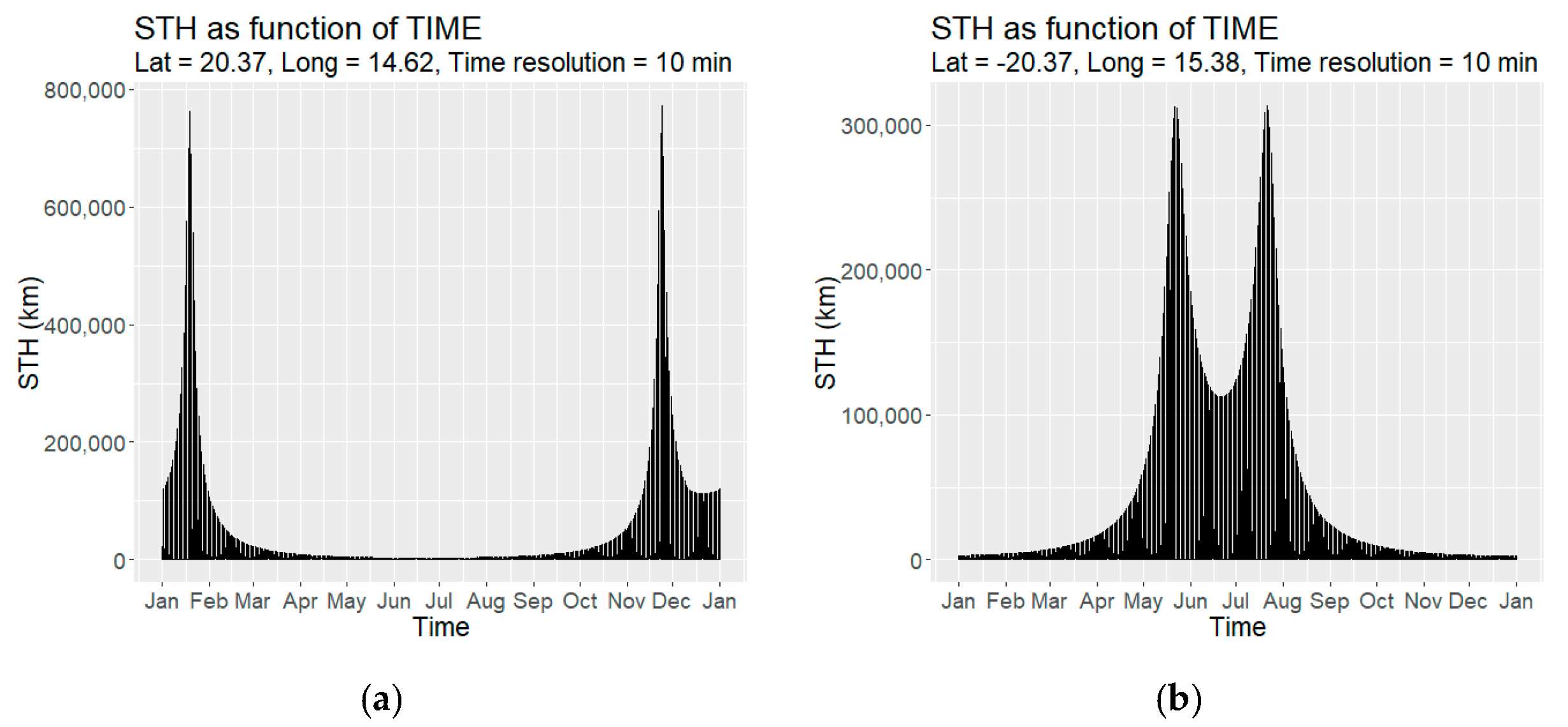
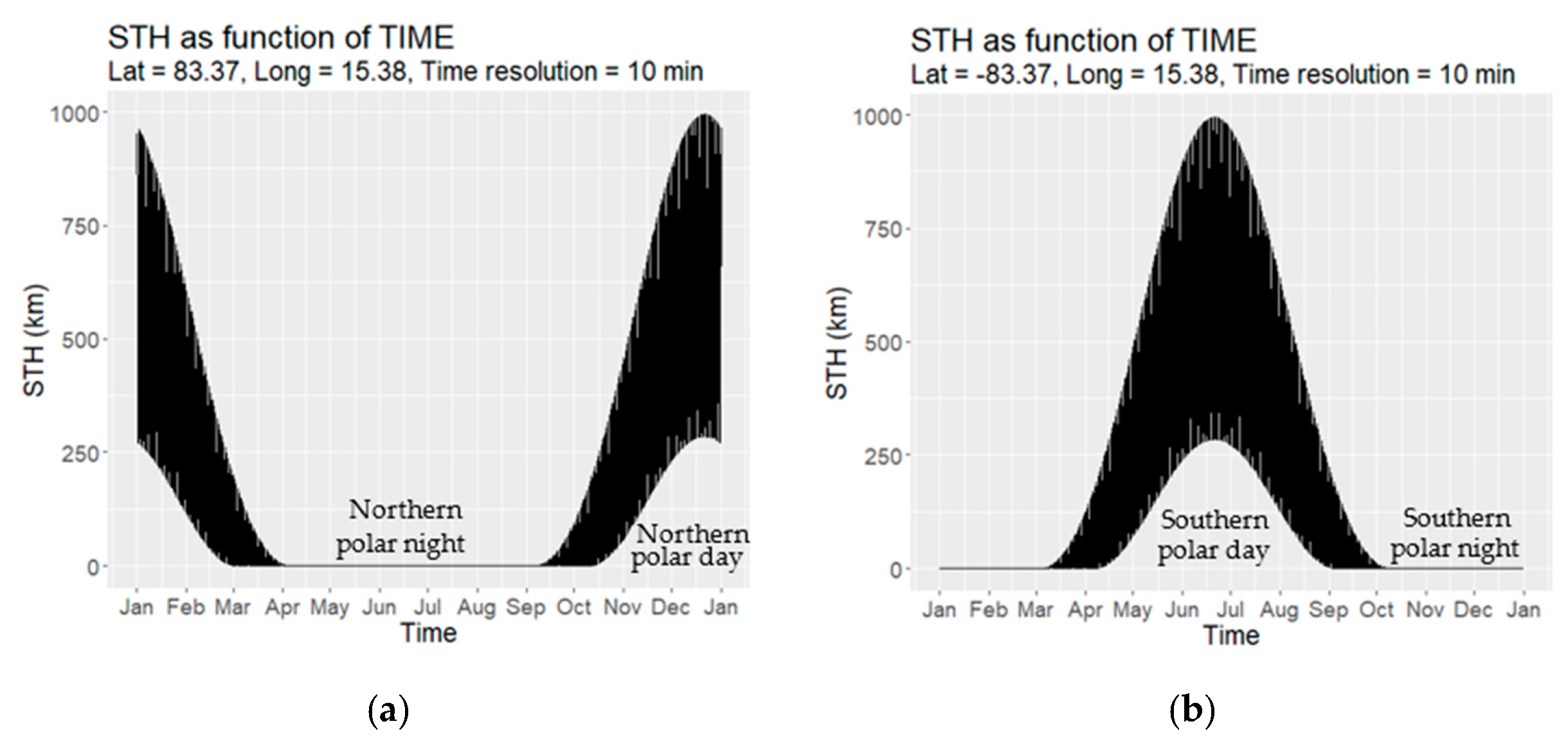
3.1. STH as Function of Time

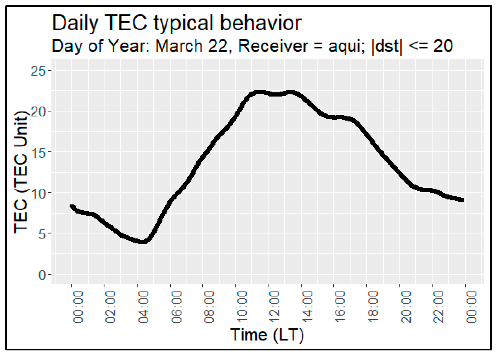
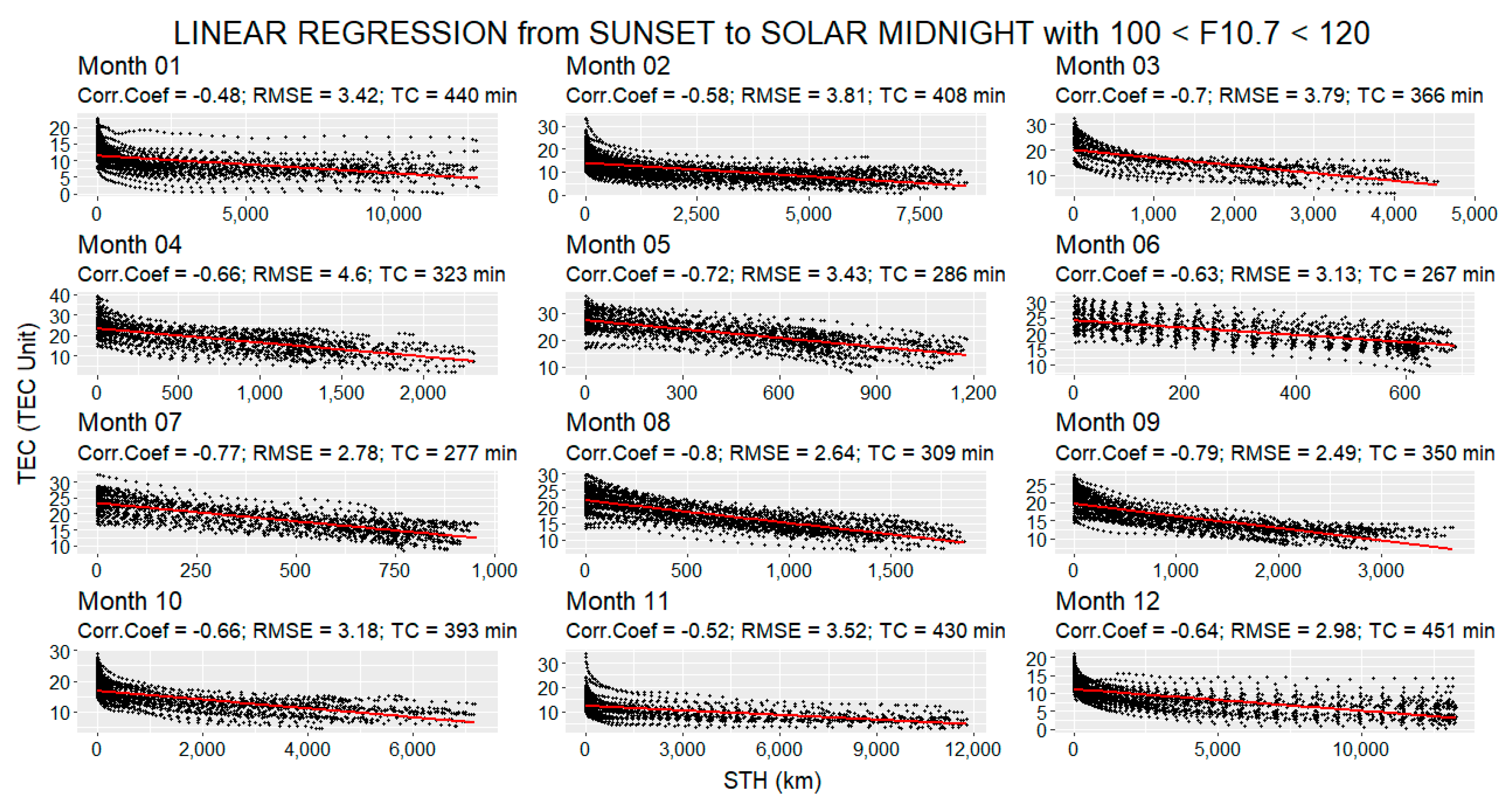
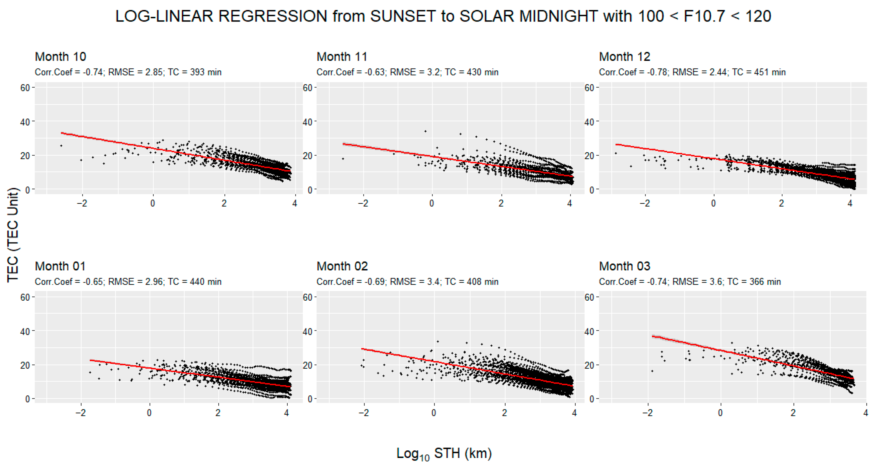
Figure 4, Figure 5 and Figure 6 give some examples of time-dependent STH values computed following the model described in Section 2.1 over three pairs of points chosen in both hemispheres in three different (Tropical, Temperate and Polar) Zones. The temporal resolution of the graphs is 10 min, and the STH values are shown for an entire year (2000).

As can be seen, the graphs proposed reflect expected STH annual behavior. In the case of the first two plots (Figure 4), relating to intertropical latitudes, the solar terminator reaches peak altitudes in the few winter nights in which the vertical to the considered geographical position is almost parallel to the direction of the Sun’s rays, going to meet the Sun-shadow line at hundreds of thousands of kilometers of altitude, before dropping abruptly. At mid-latitudes (Figure 5), however, the nocturnal peak heights show more tenuous variations, touching the maximum and minimum values at the relative winter and summer solstices. Finally, at polar latitudes, it is possible to appreciate the alternation of the months of polar day and polar night, with maximum daily values of STH that are maintained in the order of hundreds (or a few thousand) of kilometers of altitude.

3.2. STH–TEC Correlation Analysis

In this section, we show the results of a preliminary study on the STH–TEC correlation analysis during the period between sunset and solar midnight. In particular, the scatter plots and the regression lines for the two variables were monthly processed in different conditions of solar activity. As a representative example of how the correlation evolves on average in the six ranges of solar activity, we show the plots related to the solar activity level between 100 and 120 s.f.u. (Figure 7). The other five ranges of solar activity plots can be found in the Supplementary Materials to this paper (Supplementary). The TEC data used in the analysis were collected by the AQUI GPS receiver located in Central Italy (Lat.: 42.37; Long.:13.35). At the top of each graph, the corresponding linear correlation coefficient, the root mean squared error (RMSE) and the daily mean Time Coverage (TC) of the month are reported.

The statistical analysis carried out on the time interval between sunset and solar midnight highlights, as expected, a negative correlation between STH and TEC, which, albeit to a more or less marked extent, always exists. In other words, in this period of time and in the absence of high geomagnetic activity, regardless of the solar activity, it can be expected that, as the portion of the atmosphere illuminated by the sun decreases (increasing STH), the TEC also decreases.

From the visual analysis of the monthly scatter plots generated in presence of solar activity between 100 and 120 s.f.u., it is quite evident that, if on the one hand there is a fairly clear TEC–STH linear anti-correlation during the spring–summer period (in particular during the period May–August), on the other, in the autumn–winter period the decrease in TEC as STH increases is considerably more marked in the first 200–500 km of altitude, a trend that, probably, during the period September–March, can be better described with a log-linear regression (this would imply that the TEC–STH relationship is exponential).

Another element that can be seen when looking at plots individually is the tendency of TEC to decrease (as STH increases) during spring–summer months always at similar rates within the same graph (the higher the TEC at sunset, the higher the TEC at midnight). This, during this period, when the correlation tends to be linear, gives the graphs the property of homoscedasticity, a desirable property, as it implies that the errors on TEC do not vary as STH varies. However, this element allows us to assume that the correlation between the two parameters has further margins for improvement if only the causes underlying the higher or lower electronic content at sunset within the ionospheric layer could be identified. Some table checks, carried out on a sample basis, show how the initial TEC variation is only rarely attributable to slight variations in solar or geomagnetic activity within the predetermined ranges but often remains unjustified.

Given the exponential trend detected by the graphs during the autumn–winter period, a monthly log-linear regression analysis was also performed for each of the six solar activity ranges. Figure 8 shows, again by way of example, the monthly graphs of the log-linear correlation analysis for the period October–March in the same range of solar activity as in Figure 7 (100 s.f.u. < F10.7 < 120 s.f.u.). The other log-linear plots can be found in the Supplementary Materials to this paper (Supplementary 2).

The STH–TEC log-linear correlation, actually, in the solar activity range between 100 and 120 s.f.u. and during the autumn–winter period, seems to fit better than the linear one as also confirmed by the higher correlation coefficient reported at the top of the plots.

The monthly correlation coefficients obtained from each of the two analyses (linear and log-linear) and for each solar activity range are compared in

Table 2. TEC–STH correlation coefficient values for the sunset–solar midnight period obtained in each of the 12 months of the year in each of the 6 predetermined solar activity ranges and for both linear (Lin) and log-linear (Log-Lin) correlation. The values in bold are the maximums in the comparison between Lin and Log-Lin.

Linear and Log-Linear TEC–STH Correlation Coefficients Comparison
Month	F10.7 < 80		80 < F10.7 < 100		100 < F10.7 < 120		120 < F10.7 < 140		140 < F10.7 < 160		F10.7 > 160
	Lin	Log-Lin	Lin	Log-Lin	Lin	Log-Lin	Lin	Log-Lin	Lin	Log-Lin	Lin	Log-Lin
1	−0.38	−0.45	−0.55	–0.67	–0.48	–0.65	–0.60	–0.78	–0.60	–0.79	–0.45	–0.63
2	–0.45	–0.50	–0.64	–0.68	–0.58	–0.69	–0.71	–0.82	–0.69	–0.81	–0.47	–0.53
3	–0.49	–0.50	–0.66	–0.64	–0.70	–0.74	–0.70	–0.72	–0.71	–0.71	–0.67	–0.66
4	–0.66	–0.56	–0.67	–0.60	–0.66	–0.57	–0.74	–0.69	–0.71	–0.68	–0.59	–0.63
5	–0.66	–0.53	–0.61	–0.49	–0.72	–0.58	–0.78	–0.67	–0.65	–0.56	–0.77	–0.70
6	–0.69	–0.55	–0.60	–0.50	–0.63	–0.52	–0.65	–0.56	–0.72	–0.61	–0.62	–0.52
7	–0.70	–0.58	–0.66	–0.53	–0.77	–0.63	–0.76	–0.62	–0.76	–0.64	–0.63	–0.53
8	–0.64	–0.53	–0.67	–0.57	–0.80	–0.69	–0.79	–0.67	–0.78	–0.65	–0.75	–0.63
9	–0.54	–0.52	–0.65	–0.63	–0.79	–0.78	–0.61	–0.66	–0.75	–0.76	–0.64	–0.65
10	–0.44	–0.42	–0.67	–0.58	–0.66	–0.74	–0.62	–0.73	–0.69	–0.83	–0.59	–0.70
11	–0.42	–0.44	–0.58	–0.60	–0.52	–0.63	–0.59	–0.74	–0.65	–0.82	–0.55	–0.75
12	–0.39	–0.45	–0.47	–0.60	–0.64	–0.78	–0.57	–0.75	–0.62	–0.82	–0.54	–0.76

.

Adding to the visual analysis the comparison of the correlation coefficients, it appears that generally the months of March–April and September–October act as periods of transition between the two models. Instead, during the May–August and November–February periods, respectively, the linear model and the log-linear model seem to fit better. The only exception is the period October–March with F10.7 < 80 s.f.u. (very low solar activity), when neither model seems to fit well (correlation coefficients never greater than 0.5).

In

Table 3. Averages of the TEC–STH correlation coefficients of the periods May–August (linear) and November–February (log-linear), in each of the 6 predetermined solar activity ranges.

Seasonal Means of The TEC–STH Correlation Coefficients
	F10.7 < 80	80 < F10.7 < 100	100 < F10.7 < 120	120 < F10.7 < 140	140 < F10.7 < 160	F10.7 > 160
Lin (May–Aug)	−0.67	−0.64	−0.73	−0.74	−0.73	−0.69
Log-Lin (Nov–Feb)	−0.46	−0.64	−0.69	−0.77	−0.81	−0.67

, excluding the transition periods, for each of the two correlation models, are shown the seasonal means of the TEC–STH correlation coefficients of the months in which each of the two models fits better than the other (May–August for the linear one and November–February for the log-linear one).

The seasonal means of the correlation coefficients obtained with each of the two models, with the exception of the winter period in conditions of very low solar activity (F10.7 < 80), show generally good values (with correlation coefficients always greater than 0.6).

In the case of linear correlation, there is no particular trend as the solar activity varies, while in the case of log-linear correlation, as the solar activity increases the correlation coefficient also increases. The case where F10.7 is greater than 160 s.f.u. is an exception showing a reduction of the log-linear correlation coefficient likely due to the major weights assumed by F10.7 outliers compared with a reduced population of records.

4. Discussion

The availability of an accurate solar illumination model of the Earth’s atmosphere could be functional to the improvement of studies relating to the whole series of applications (AGW/TID, vertical pressure and temperature profiles, neutral and ionic atmospheric components, electromagnetic waves, total electron content, ionospheric empirical models, etc.) already discussed in the introductory section.

The TEC–STH dependence relationships that were determined, on the other hand, have the ultimate aim of describing and better predicting the nocturnal behavior of the TEC parameter to obtain useful information for improving the processing of empirical models and forecasting models. In this sense, also given the absence of previous studies on the same topic, the investigation initiated represents a starting point for proceeding to more detailed analyses that can open up different directions of research.

This first STH–TEC correlation analysis seems to indicate that, in the absence of geomagnetic activity and in the post-sunset hours, the trend with which the TEC decreases, as the portion of the ionosphere illuminated by the sun decreases, tends to be linear during the summer period and exponential during the winter period. The exponential decreasing trend is best suited in conditions of high solar activity.

The fact that the TEC has a decreasing trend (as STH increases) always at similar rates within the monthly time intervals during the spring/summer period suggests that the relationship could be also investigated by a multivariate regression analysis involving other potential covariates (e.g., vertical temperature profile, portion of the atmosphere crossed by incident solar radiation, Sun’s declination angle, etc.).

References

1. Beer, T. Supersonic Generation of Atmospheric Waves. Nature 1973, 242, 34. [Google Scholar] [CrossRef]
2. Dominici, P.; Bianchi, C.; Cander, L.; De Francheschi, G.; Scotto, C.; Zolesi, B. Preliminary results on the ionospheric structure at dawn time observed during HRIS campaigns. Ann. Geophys. 1994, 37, 71–76. [Google Scholar] [CrossRef]
3. Vasilyev, V.P. Latitude location of the source of the ionospheric short-term terminator disturbances. Geomag. Aeron. 1996, 35, 589. [Google Scholar]
4. Galushko, V.G.; Paznukhov, V.V.; Yampolski, Y.M.; Foster, J.C. Incoherent scatter radar observations of AGW/TID events generated by the moving solar terminator. Ann. Geophys. 1998, 16, 821–827. [Google Scholar] [CrossRef]
5. Afraimovich, E.L.; Edemskiy, I.K.; Leonovich, A.S.; Leonovich, L.A.; Voeykov, S.V.; Yasyukevich, Y.V. MHD nature of night-time MSTIDs excited by the solar terminator. Geophys. Res. Lett. 2009, 36. [Google Scholar] [CrossRef] [Green Version]
6. MacDougall, J.; Jayachandran, P. Solar terminator and auroral sources for traveling ionospheric disturbances in the midlatitude F region. J. Atmos. Sol. Terr. Phys. 2011, 73, 2437–2443. [Google Scholar] [CrossRef]
7. Fowler, D.; Pilegaard, K.; Sutton, M.; Ambus, P.; Raivonen, M.; Duyzer, J.; Simpson, D.; Fagerli, H.; Fuzzi, S.; Schjoerring, J.; et al. Atmospheric composition change: Ecosystems–Atmosphere interactions. Atmos. Environ. 2009, 43, 5193–5267. [Google Scholar] [CrossRef]
8. Karpov, I.V.; Bessarab, F.S. Model studying the effect of the solar terminator on the thermospheric parameters. Geomagn. Aeron. 2008, 48, 209–219. [Google Scholar] [CrossRef]
9. Afraimovich, E.L.; Edemskiy, I.K.; Voeykov, S.V.; Yasyukevich, Y.V.; Zhivetiev, I.V. The first GPS-TEC imaging of the space structure of MS wave packets excited by the solar terminator. Ann. Geophys. 2009, 27, 1521–1525. [Google Scholar] [CrossRef]
10. Bespalova, A.V.; Fedorenko, A.; Cheremnykh, O.; Zhuk, I. Satellite observations of wave disturbances caused by moving solar TERMINATOR. J. Atmos. Sol. Terr. Phys. 2016, 140, 79–85. [Google Scholar] [CrossRef]
11. Pignalberi, A.; Habarulema, J.; Pezzopane, M.; Rizzi, R. On the Development of a Method for Updating an Empirical Climatological Ionospheric Model by Means of Assimilated vTEC Measurements from a GNSS Receiver Network. Space Weather 2019, 17, 1131–1164. [Google Scholar] [CrossRef] [Green Version]
12. Verhulst, T.G.W.; Stankov, S.M. Height-dependent sunrise and sunset: Effects and implications of the varying times of occurrence for local ionospheric processes and modelling. Adv. Space Res. 2017, 60, 1797–1806. [Google Scholar] [CrossRef]
13. Kintner, P.M.; Ledvina, B.M. The ionosphere, radio navigation, and global navigation satellite systems. Adv. Space Res. 2005, 35, 788–811. [Google Scholar] [CrossRef]
14. Rocken, C.; Kuo, Y.H.; Schreiner, W.S.; Hunt, D.; Sokolovskiy, S.; McCormick, C. COSMIC System Description. Terr. Atmos. Ocean. Sci. 2000, 11, 21–52. [Google Scholar] [CrossRef] [Green Version]
15. Hajj, G.A.; Lee, L.C.; Pi, X.; Romans, L.J.; Schreiner, W.S.; Straus, P.R.; Wang, C. COSMIC GPS Ionospheric Sensing and Space Weather. Terr. Atmos. Ocean. Sci. 2000, 11, 235–272. [Google Scholar] [CrossRef] [Green Version]
16. Parrot, M. The micro-satellite DEMETER. J. Geodyn. 2002, 33, 535–541. [Google Scholar] [CrossRef]
17. Tiwari, R.; Bhattacharya, S.; Purohit, P.K.; Gwal, A.K. Effect of TEC Variation on GPS Precise Point at Low Latitude. Open Atmos. Sci. J. 2009, 3, 1–12. [Google Scholar] [CrossRef] [Green Version]
18. Fayose, R.S.; Babatunde, R.; Oladosu, O.; Groves, K. Variation of Total Electron Content [TEC] and Their Effect on GNSS over Akure, Nigeria. Appl. Phys. Res. 2012, 4, 105. [Google Scholar] [CrossRef] [Green Version]
19. Freund, F. Pre-earthquake signals: Underlying physical processes. J. Asian Earth Sci. 2011, 41, 383–400. [Google Scholar] [CrossRef]
20. Pulinets, S.; Ouzounov, D. Lithosphere—Atmosphere—Ionosphere Coupling (LAIC) model—An unified concept for earthquake precursors validation. J. Asian Earth Sci. 2011, 41, 371–382. [Google Scholar] [CrossRef]
21. Kuo, C.L.; Huba, J.D.; Joyce, G.; Lee, L.C. Ionosphere plasma bubbles and density variations induced by pre-earthquake rock currents and associated surface charges. J. Geophys. Res. Space Phys. 2011, 116. [Google Scholar] [CrossRef] [Green Version]
22. Kuo, C.L.; Lee, L.C.; Huba, J.D. An improved coupling model for the lithosphere-atmosphere-ionosphere system. J. Geophys. Res. Space Phys. 2014, 119, 3189–3205. [Google Scholar] [CrossRef]
23. Yang, S.; Asano, T.; Hayakawa, M. Abnormal Gravity Wave Activity in the Stratosphere Prior to the 2016 Kumamoto Earthquakes. J. Geophys. Res. Space Phys. 2019, 124, 1410–1425. [Google Scholar] [CrossRef]
24. Meeus, J. Astronomical Algorithms, 2nd ed.; Willmann-BeIl Inc.: Richmond, VA, USA, 1998. [Google Scholar]
25. NOAA. Solar Calculation Details. Available online: https://www.esrl.noaa.gov/gmd/grad/solcalc/calcdetails.html (accessed on 8 April 2021).
26. Astronomical Almanac for the Year 2010 and Its Companion the Astronomical Almanac Online. Available online: http://www.admiraltyshop.co.uk (accessed on 8 April 2021).
27. R Core Team. R: A Language and Environment for Statistical Computing; R Foundation for Statistical Computing: Vienna, Austria, 2013; Available online: http://www.R-project.org/ (accessed on 8 April 2021).
28. Eyelade, V.A.; Adewale, A.O.; Akala, A.O.; Bolaji, O.S.; Rabiu, A.B. Studying the variability in the diurnal and seasonal variations in GPS total electron content over Nigeria. Ann. Geophys. 2017, 35, 701–710. [Google Scholar] [CrossRef] [Green Version]
29. Yuen, P.; Roelofs, T. Seasonal variations in ionospheric total electron content. J. Atmos. Sol. Terr. Phys. 1967, 29, 321–326. [Google Scholar] [CrossRef]
30. Zhao, B.; Wan, W.; Liu, L.; Mao, T.; Ren, Z.; Wang, M.; Christensen, A.B. Features of annual and semiannual variations derived from the global ionospheric maps of total electron content. Ann. Geophys. 2007, 25, 2513–2527. [Google Scholar] [CrossRef] [Green Version]
31. Tsai, H.-F.; Liu, J.-Y.; Tsai, W.-H.; Liu, C.-H.; Tseng, C.-L.; Wu, C.-C. Seasonal variations of the ionospheric total electron content in Asian equatorial anomaly regions. J. Geophys. Res. Space Phys. 2001, 106, 30363–30369. [Google Scholar] [CrossRef]
32. Perevalova, N.; Polyakova, A.; Zalizovski, A. Diurnal variations of the total electron content under quiet helio-geomagnetic conditions. J. Atmos. Sol. Terr. Phys. 2010, 72, 997–1007. [Google Scholar] [CrossRef]
33. IONOLAB. Available online: http://www.ionolab.org/index.php?page=ionolabtec&language=en (accessed on 9 February 2021).
34. Sezen, U.; Arikan, F.; Arikan, O.; Ugurlu, O.; Sadeghimorad, A. Online, automatic, near-real time estimation of GPS-TEC: IONOLAB-TEC. Space Weather 2013, 11, 297–305. [Google Scholar] [CrossRef]
35. Arikan, F.; Nayir, H.; Sezen, U.; Arikan, O. Estimation of single station interfrequency receiver bias using GPS-TEC. Radio Sci. 2008, 43, 4. [Google Scholar] [CrossRef]
36. OMINWeb. Available online: https://omniweb.gsfc.nasa.gov/form/dx1.html (accessed on 8 April 2021).
Figure 1. Solar illumination model of the Earth’s ellipsoid at the time of the equinox and representation of the ellipsoidal height of the solar terminator (Solar Terminator Height) h and of some of the related parameters.
Earth 02 00012 g001
Figure 2. Solar illumination model of the Earth’s ellipsoid at the time of the Northern Hemisphere winter solstice and representation of the ellipsoidal height of the solar terminator (Solar Terminator Height) h, of the declination angle δ and of some of the related parameters.
Earth 02 00012 g002
Figure 3. TEC measurements collected by the GPS L’Aquila receiver (Central Italy) on 22 March 2016 showing the fairly standard behavior of TEC at mid-latitudes (in quiet geomagnetic activity conditions).
Earth 02 00012 g003
Figure 4. Examples of time-dependent STH determination by using the proposed model. The two figures show the trend of STH as a function of time over an entire year (2000) in tropical latitudes. Figure (a) represents STH in the Northern Hemisphere. Figure (b) represents STH in the Southern Hemisphere. Note that, in the two STH peaks—corresponding to the solar midnight of the two days of the year in which the latitude θ is closest to −δ (declination)—small variations in computation time or longitude are enough to ensure that each of the two STH peaks varies considerably (in fact, if it were θ = −δ, when SZA = −180, it would be STH = ). Therefore, precise longitude values were chosen, such as to better emphasize such an aspect.
Earth 02 00012 g004
Figure 5. Examples of time-dependent STH determination by using the proposed model. The two figures show the trend of STH as a function of time over an entire year (2000) in temperate latitudes. Figure (a) represents STH in the Northern Hemisphere. Figure (b) represents STH in the Southern Hemisphere.
Earth 02 00012 g005
Figure 6. Examples of time-dependent STH determination by using the proposed model. The two figures show the trend of STH as a function of time over an entire year (2000) in polar latitudes. Figure (a) represents STH in the Northern Hemisphere. Figure (b) represents STH in the Southern Hemisphere.
Earth 02 00012 g006
Figure 7. The 12 graphs show the TECSTH scatter plots and the related linear regression line of 20 years (2000–2019) of data grouped by month, with solar activity level between 100 and 120 s.f.u., under quiet geomagnetic conditions and in the time interval between sunset and solar midnight. The linear correlation coefficient, the root mean squared error and the daily mean Time Coverage (TC) of the month are shown at the top of the graphs.
Earth 02 00012 g007
Figure 8. The 6 graphs show the TECSTH scatter plots and the related log-linear regression line of 20 years (2000–2019) of data grouped by month, for the period October–March, with solar activity level between 100 and 120 s.f.u., under quiet geomagnetic conditions and in the time interval between sunset and solar midnight. The log-linear correlation coefficient, the root mean squared error and the daily mean Time Coverage (TC) of the month are shown at the top of the graphs.
Earth 02 00012 g008