A Hybrid Deep Learning Framework for Smart Grid Stress Prediction and Adaptive Mitigation Under Extreme Weather Conditions

Abstract

Electricity systems are increasingly exposed to demand variability driven by extreme weather conditions, creating significant challenges for maintaining grid reliability and operational stability. Conventional forecasting approaches focus primarily on prediction accuracy and provide limited support for operational decision-making under dynamic conditions. This study proposes a hybrid deep learning framework for smart grid stress prediction and adaptive mitigation under extreme weather. The framework reformulates demand forecasting using residual learning. It further integrates grid stress modelling with control-oriented decision support. A sequence learning architecture with attention is employed to capture temporal demand dynamics, while a continuous Grid Stress Index (GSI) translates predictions into operational indicators of system stress. The model demonstrates stable performance on real-world UK electricity demand data, achieving a mean absolute error of 1827.51 MW and a root mean squared error of 2505.22 MW. Peak demand and ramp behaviour are captured with improved consistency, and grid stress is predicted with a mean absolute error of 0.1246. An adaptive mitigation module translates predicted stress into actionable control, resulting in approximately 5.37% peak demand reduction, with limited impact on ramp smoothing. The results demonstrate that integrating forecasting, stress modelling, and control delivers greater operational value than standalone predictive models. The proposed framework provides a scalable and practical approach for grid-aware decision support under increasing climate-driven demand uncertainty.

1. Introduction

Electricity systems are undergoing a structural transformation driven by the rapid integration of renewable energy sources, electrification of transport and heating, and increasing climate variability [1]. These developments introduce significant operational complexity, requiring power systems to operate under more dynamic and uncertain conditions. In particular, maintaining system reliability now depends on the ability to anticipate and respond to rapid fluctuations in electricity demand and supply [2,3].

Short-term electricity demand forecasting remains a fundamental component of grid operation, supporting generation scheduling, reserve allocation, and market operations [4,5]. Traditional forecasting approaches have evolved from statistical models such as autoregressive integrated moving average (ARIMA) to machine learning and deep learning methods capable of capturing nonlinear temporal dependencies [6]. Recent advances in deep learning, particularly Long Short-Term Memory (LSTM) networks and hybrid architectures, have demonstrated strong performance in modelling complex demand patterns [7,8,9].

Despite these advances, a critical limitation persists. Most forecasting models are optimised for prediction accuracy as an end objective, with limited consideration of how forecasts are used in operational decision-making. In practical grid environments, accurate prediction alone is insufficient [10]. System operators require interpretable and actionable indicators that reflect grid stress, risk, and operational constraints. This gap between predictive modelling and operational utility has been increasingly recognised in recent research on resilient power systems [11,12].

The challenge is further amplified under extreme weather conditions. Heatwaves, cold spells, and severe meteorological events significantly alter electricity demand patterns while simultaneously affecting generation availability and network performance [13,14,15]. These conditions introduce non-stationarity and increased uncertainty, reducing the effectiveness of conventional forecasting models [16,17]. As climate-driven variability intensifies, the ability to model and manage extreme demand behaviour becomes a critical requirement for grid resilience [18,19,20].

Recent studies have explored hybrid deep learning architectures, including convolutional neural network–long short-term memory (CNN–LSTM) and transformer-based models, to improve forecasting performance under complex conditions [21,22]. While these approaches enhance predictive capability, they remain largely prediction-centric and do not explicitly incorporate grid stress assessment or control-oriented decision mechanisms. This reveals three key limitations in the current state of research. First, forecast outputs are rarely translated into operational indicators that quantify system stress or risk. Second, model evaluation is typically conducted under average conditions, with limited emphasis on extreme demand events where operational decisions are most critical. Third, there is minimal integration between forecasting models and adaptive control strategies that can mitigate predicted stress conditions in real time.

Addressing these limitations requires a shift from prediction-centric modelling toward integrated predictive–control frameworks. Such frameworks extend forecasting beyond accuracy metrics by embedding it within a broader decision-support architecture that includes stress quantification and mitigation [23,24,25,26]. This study proposes a hybrid deep learning framework for smart grid stress prediction and adaptive mitigation under extreme weather conditions. The approach reformulates electricity demand forecasting as a residual learning problem and integrates it with grid stress modelling and control-oriented decision-making. A sequence learning architecture with attention is used to capture temporal demand dynamics, while a continuous Grid Stress Index (GSI) translates forecasts into operational indicators of system conditions.

Novelty and Contributions

By linking prediction with stress assessment and state-driven mitigation, the proposed framework enables proactive management of grid conditions under weather-driven demand variability and provides a practical pathway for improving grid resilience. This work differs from existing studies in three fundamental ways. First, forecasting is reformulated as a residual learning problem to explicitly model deviations under extreme conditions, rather than absolute demand. Second, grid stress is introduced as a continuous, learnable operational variable within a multi-task learning framework, rather than a post hoc indicator. Third, prediction outputs are directly embedded within a closed-loop mitigation mechanism, enabling operational decision support rather than passive forecasting.

2. Related Work

Electricity demand forecasting has been extensively studied, with approaches broadly categorised into statistical models, machine learning methods, and deep learning architectures. Statistical and machine learning approaches were used in previous work on electricity demand forecasting, and some relied on autoregressive integrated moving average (ARIMA) and seasonal variants [27,28,29,30]. These models provide interpretable and computationally efficient solutions, but are limited in their ability to capture nonlinear dependencies and complex interactions between demand drivers [6].

To address these limitations, machine learning techniques such as support vector regression, decision trees, and ensemble methods have been applied to load forecasting [31]. These approaches improve nonlinear modelling capability but often require extensive feature engineering and still struggle to capture long-range temporal dependencies inherent in electricity demand data [6].

Deep learning-based forecasting has emerged as the dominant approach for short-term load forecasting due to its ability to learn hierarchical representations directly from data. Recurrent neural networks, particularly Long Short-Term Memory (LSTM) models, have demonstrated strong performance in capturing temporal dependencies in electricity demand [4,7]. Hybrid architectures further enhance performance by combining complementary modelling capabilities. For example, CNN–LSTM models integrate convolutional layers for feature extraction with recurrent layers for sequence learning, enabling improved representation of spatiotemporal patterns [8,21,32]. More recently, transformer-based models have been introduced to capture long-range dependencies using attention mechanisms [22,33,34]. Despite these advances, most deep learning approaches remain focused on improving forecast accuracy. They typically treat demand prediction as an isolated task, without explicitly considering how predictions are utilised in grid operation.

The impact of extreme weather on electricity demand has gained increasing attention in recent years. Studies show that heatwaves, cold spells, and other meteorological extremes introduce significant deviations from normal demand patterns, increasing the uncertainty in forecasting [16,17]. To address this, hybrid models have been proposed to incorporate meteorological variables such as temperature, wind speed, and solar irradiance. These approaches improve the sensitivity of models to weather-driven demand variability and enhance forecast performance under abnormal conditions [17,35].

Recent research has begun to explore the integration of forecasting with grid resilience and operational decision-making. Frameworks that combine source–load coordination and system-level modelling aim to support proactive grid management under uncertainty [11,12]. These approaches represent a shift toward grid-aware forecasting, where predictions are used to inform operational strategies. However, existing work remains fragmented. Forecasting, stress assessment, and control are often developed as separate components, with limited end-to-end integration.

The review of existing literature reveals a persistent disconnect between predictive modelling and operational decision-making in smart grid systems. Most forecasting approaches are designed to optimise predictive accuracy as an end objective, without explicitly linking model outputs to operational indicators that reflect grid stress or system risk. In addition, model evaluation is typically conducted under average operating conditions, with limited emphasis on extreme demand scenarios where system vulnerability is highest. These limitations highlight the need for an integrated framework that extends forecasting beyond accuracy metrics toward actionable operational intelligence. In response, this study proposes a unified predictive–control architecture that reformulates electricity demand forecasting using residual learning, incorporates grid stress modelling through a continuous Grid Stress Index, and integrates adaptive mitigation strategies within a closed-loop decision-support system. Unlike existing approaches, the proposed framework explicitly links prediction, stress quantification, and control, enabling proactive management of peak demand and system stress under extreme weather conditions.

3. Methodology

The proposed framework is designed to extend conventional electricity demand forecasting into a grid-aware predictive system that captures both demand dynamics and operational stress conditions. Rather than directly predicting electricity demand, the problem is reformulated using a residual learning paradigm and a multi-task learning strategy. This enables the model to simultaneously learn demand deviations and grid stress behaviour under weather-driven variability.

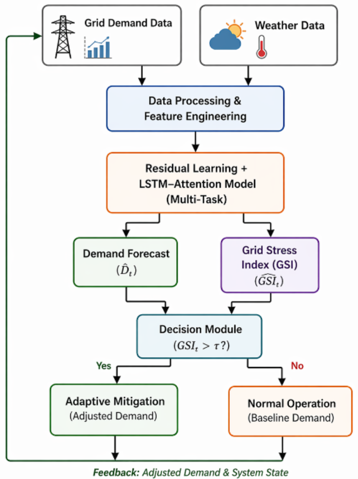
The methodology consists of four interconnected components: data acquisition and preprocessing, feature engineering and residual formulation, hybrid sequence learning, and grid stress modelling. The system-level architecture of the proposed framework is illustrated in Figure 1. The design follows a modular structure in which each component performs a distinct functional role while contributing to a unified predictive–control loop.

The data processing module transforms raw demand and meteorological inputs into structured features. The forecasting engine generates residual demand and grid stress predictions using a hybrid LSTM–attention model. These predictions are passed to the grid stress evaluation module, which converts them into operational indicators. The adaptive control module then applies mitigation actions based on predicted stress levels.

Unlike conventional forecasting pipelines, the proposed architecture establishes a closed-loop interaction between prediction and control. This establishes a closed-loop predictive–control pipeline aligned with real-time grid operation.

3.1. Data Acquisition and Preprocessing

The framework utilises real-world electricity demand data obtained from the UK National Grid Electricity System Operator (ESO), and meteorological data provided by the European Centre for Medium-Range Weather Forecasts (ECMWF) Reanalysis v5 (ERA5) [36]. The demand data consist of half-hourly measurements, while ERA5 provides high-resolution atmospheric variables. The electricity demand at time t is denoted by $D_t$, and the corresponding vector of weather features is defined by (1), where $T_t$, $V_t$, and $S_t$ represent temperature, wind speed and solar irradiance, respectively.

$$W_t=[T_t,V_t,S_t]$$

(1)

3.2. Feature Engineering and Temporal Encoding

To capture cyclical behaviour in electricity demand, temporal features are encoded using sinusoidal transformations. The hour-of-day encoding, defined in (2) is used. Similarly, day-of-week encoding is defined in (3), where h represents hour-of-day and d represents day-of-week.

$${\mathrm{hour}}_{sin}=sin\left({\displaystyle \frac{2\pi h}{24}}\right),{\mathrm{hour}}_{cos}=cos\left({\displaystyle \frac{2\pi h}{24}}\right)$$

(2)

$${\mathrm{dow}}_{sin}=sin\left({\displaystyle \frac{2\pi d}{7}}\right),{\mathrm{dow}}_{cos}=cos\left({\displaystyle \frac{2\pi d}{7}}\right)$$

(3)

To capture temporal dependencies, lagged demand features are constructed as defined in (4). Short-term variability is captured using rolling statistics and the rolling mean and standard deviation are defined in (5). These engineered features allow the model to represent both periodic demand patterns and short-term fluctuations.

$${\mathcal{L}}_t=[D_{t-1},D_{t-2},D_{t-24},D_{t-96},D_{t-336}]$$

(4)

$${\mu }_t^{\left(k\right)}={\displaystyle \frac{1}{k}}{\displaystyle \sum _{i=0}^{k-1}}{D}_{t-i},{\sigma }_t^{\left(k\right)}=\sqrt{{\displaystyle \frac{1}{k}}\sum _{i=0}^{k-1}{(D_{t-i}-{\mu }_t^{\left(k\right)})}^2}$$

(5)

3.3. Residual Learning Formulation

To reduce learning complexity, electricity demand is decomposed into a baseline component and a residual component. This decomposition is defined in (6), where $B_t$ represents a persistence-based baseline and $R_t$ represents the residual deviation. The baseline component is defined using daily persistence in (7), and the residual component is obtained from (8). This formulation allows the model to focus on deviations from expected demand behaviour rather than learning the full signal. Residual learning has been shown to improve convergence and stability in time-series forecasting [4].

$$D_t=B_t+R_t$$

(6)

$$B_t=D_{t-48}$$

(7)

$$R_t=D_t-B_t$$

(8)

3.4. Hybrid Sequence Learning Model

The temporal learning component is implemented using a Long Short-Term Memory (LSTM) network with an attention mechanism. Given an input sequence $X_{t-k:t}$, the LSTM produces a sequence of hidden states as defined in (9). An attention mechanism is applied to compute the importance weights of each time step and the weights are defined in (10).

$$H=[h_1,h_2,\dots ,h_k]$$

(9)

$${\alpha }_i={\displaystyle \frac{exp\left(W{h}_i\right)}{{\sum }_{j}exp\left(W{h}_j\right)}}$$

(10)

The context vector is then computed as a weighted sum of hidden states, as shown in (11). This mechanism enables the model to selectively focus on relevant temporal patterns when generating predictions.

$$c=\sum _i{\alpha }_i{h}_i$$

(11)

3.5. Multi-Task Learning for Demand and Grid Stress Prediction

The model is trained using a multi-task formulation to jointly predict residual demand ${\widehat{R}}_t$ and grid stress ${\widehat{GSI}}_t$, with demand reconstructed using (12). To quantify operational conditions, a Grid Stress Index (GSI) is defined in (13), where ${\lambda }_1$ and ${\lambda }_2$ are weighting coefficients. The GSI is formulated as a continuous operational proxy that captures two dominant drivers of system stress: demand magnitude, which reflects proximity to peak capacity and reserve margin constraints, and short-term demand variability, which represents ramping requirements and operational instability.

This formulation is consistent with recent developments in grid-aware energy management systems, where forecasting outputs are increasingly coupled with control-oriented decision layers to enable proactive system operation [37,38]. In such frameworks, system stress is treated as a control-relevant signal rather than a descriptive metric, enabling direct integration of predictive models within operational decision-making pipelines.

A linear combination of normalised demand and ramp-based variability is adopted to ensure computational tractability and real-time applicability, while preserving interpretability for system operators. The weighting coefficients ${\lambda }_1$ and ${\lambda }_2$ are selected to balance steady-state loading effects and transient dynamics, ensuring consistent scaling across operating regimes. By embedding GSI within the learning objective, the proposed framework enables the model to internalise system stress behaviour during training, effectively bridging the gap between predictive modelling and operational decision support under dynamic and weather-driven conditions.

$${\widehat{D}}_t=B_t+{\widehat{R}}_t$$

(12)

$$GS{I}_t={\lambda }_1{\displaystyle \frac{D_t}{max\left(D_{t-k:t}\right)}}+{\lambda }_2{\displaystyle \frac{|D_t-D_{t-1}|}{{\sigma }_t^{\left(k\right)}}}$$

(13)

During training, $GS{I}_t$ is computed using observed demand $D_t$, while during inference, it is evaluated using predicted demand ${\widehat{D}}_t$ to ensure consistency with real-time deployment conditions. Algorithm 1 outlines the proposed pipelines for the forecast and stress prediction.

Algorithm 1: Grid-Aware Demand Forecasting and Stress Prediction Pipeline

Require:  Demand data $D_t$, weather data $W_t$ Ensure:  Predicted demand ${\widehat{D}}_t$, predicted stress ${\widehat{GSI}}_t$  1: Align and clean demand and weather data  2: Construct feature vector $X_t=[W_t,C_t,{\mathcal{L}}_t,{\mu }_t^{\left(k\right)},{\sigma }_t^{\left(k\right)}]$  3: Compute baseline demand: $$B_t=D_{t-48}$$  4: Compute residual: $$R_t=D_t-B_t$$  5: Normalise input features and residuals  6: Construct input sequences: $${\mathbf{X}}_t=[X_{t-k+1},\dots ,X_t]$$  7: Train LSTM-attention model to minimise: $$\mathcal{L}=\alpha {\mathcal{L}}_{res}+\beta {\mathcal{L}}_{gsi}+\gamma {\mathcal{L}}_{ramp}$$  8: Predict residual ${\widehat{R}}_t$ and stress ${\widehat{GSI}}_t$  9: Reconstruct demand: $${\widehat{D}}_t=B_t+{\widehat{R}}_t$$   10:  return ${\widehat{D}}_t$, ${\widehat{GSI}}_t$

3.6. Loss Function and Optimisation

The model is trained using a composite loss function that integrates residual prediction, grid stress prediction, and ramp consistency. The total loss is defined in (14), with individual components given in (15)–(17). The weighting coefficients $\alpha$, $\beta$, and $\gamma$ control the relative contribution of each component and are empirically selected to balance forecasting accuracy and temporal consistency.

$$\mathcal{L}=\alpha {\mathcal{L}}_{res}+\beta {\mathcal{L}}_{gsi}+\gamma {\mathcal{L}}_{ramp}$$

(14)

$${\mathcal{L}}_{res}=|R_t-{\widehat{R}}_t|$$

(15)

$${\mathcal{L}}_{gsi}=|GS{I}_t-{\widehat{GSI}}_t|$$

(16)

$${\mathcal{L}}_{ramp}=|(R_t-R_{t-1})-({\widehat{R}}_t-{\widehat{R}}_{t-1})|$$

(17)

Model parameters are updated using gradient-based optimisation as defined in (18), where $\eta$ is the learning rate.

$${\theta }_{t+1}={\theta }_t-\eta {\nabla }_{\theta }\mathcal{L}$$

(18)

The proposed framework introduces three key innovations. First, the forecast of electricity demand is reformulated using residual learning, which improves stability and reduces the complexity of the model. Second, grid stress is incorporated as a learnable target through multi-task learning. Third, ramp dynamics are explicitly modelled within the loss function to capture operational behaviour. These design choices enable the framework to move beyond accuracy-focused prediction toward operationally meaningful forecasting, supporting grid-aware decision-making under extreme weather conditions.

4. System Design and Implementation

The proposed framework is implemented as a modular pipeline that integrates data processing, sequence learning, grid stress evaluation, and adaptive mitigation. The design emphasises scalability, reproducibility, and clear separation of functional components, enabling both independent validation and end-to-end deployment. Figure 1 illustrates the overall system architecture, where each module transforms inputs into progressively more operationally meaningful representations.

4.1. Data Processing Module

The data processing module transforms raw electricity demand and meteorological data into structured model inputs. At each time step t, the feature set comprises meteorological variables $W_t=[T_t,V_t,S_t]$, calendar features $C_t$ encoding hour-of-day and day-of-week as defined in (2) and (3), lagged demand features ${\mathcal{L}}_t$ defined in (4), and rolling statistical descriptors ${\mu }_t^{\left(k\right)}$ and ${\sigma }_t^{\left(k\right)}$ defined in (5). The complete feature vector is constructed as given in (19). This representation captures environmental drivers, temporal structure, and short-term demand dynamics within a unified input space.

$$X_t=[W_t,C_t,{\mathcal{L}}_t,{\mu }_t^{\left(k\right)},{\sigma }_t^{\left(k\right)}]$$

(19)

To ensure numerical stability and efficient training, each feature is standardised using statistics computed from the training set. The normalised feature is given by (20), where ${\mu }_x$ and ${\sigma }_x$ denote the mean and standard deviation of feature x. This standardisation ensures that all features are centred and scaled consistently across training, validation, and test sets.

$$x^{norm}={\displaystyle \frac{x-{\mu }_x}{{\sigma }_x}}$$

(20)

4.2. Sequence Construction

The forecasting model operates on fixed-length temporal sequences. Given a sequence length k, the input to the model is constructed as a rolling window of past observations, as defined in (21). The corresponding prediction targets are defined at the next time step. Specifically, the model predicts the residual demand $R_{t+1}$, defined in (8), and the grid stress index $GS{I}_{t+1}$, defined in (13). This formulation enables the model to learn temporal dependencies over a rolling window of historical observations while simultaneously capturing demand dynamics and system stress behaviour.

$${\mathbf{X}}_t=[X_{t-k+1},X_{t-k+2},\dots ,X_t]$$

(21)

4.3. Forecasting Engine

The forecasting engine implements the hybrid sequence learning model described in the methodology. The model consists of three main components: an LSTM encoder, an attention mechanism, and dual output heads. Given the input sequence ${\mathbf{X}}_t$, the LSTM encoder produces hidden states as defined in (9). The attention mechanism then computes a context vector c using (11), which captures the most relevant temporal information for prediction.

The model generates two outputs: the predicted residual demand and the predicted grid stress index, defined in (22) and (23), where $f_{res}(·)$ and $f_{gsi}(·)$ are fully connected layers that map the context vector to residual and stress predictions, respectively. The model jointly predicts residual demand and grid stress through dual output heads.

$${\widehat{R}}_{t+1}=f_{res}\left(c\right)$$

(22)

$${\widehat{GSI}}_{t+1}=f_{gsi}\left(c\right)$$

(23)

4.4. Grid Stress Evaluation Engine

The grid stress evaluation module converts predicted demand into operational indicators. Given the predicted demand ${\widehat{D}}_t$ from (12), three key indicators are computed: peak demand ratio, ramp rate, and normalised volatility.

The peak demand ratio is defined in (24) and quantifies how close the current demand is to the recent maximum levels, where $max\left({\widehat{D}}_{t-k:t}\right)$ represents the maximum predicted demand over a rolling window. The ramp rate is defined in (25) and measures the magnitude of demand change between consecutive time steps. Demand volatility is characterised using a rolling standard deviation. The normalised volatility is defined in (26), where ${\sigma }_t^{\left(k\right)}$ is given by (5). These indicators are combined to compute the Grid Stress Index as defined in (13). The resulting index provides a continuous measure of system stress and can be used to identify different operational regimes.

$$R_{peak,t}={\displaystyle \frac{{\widehat{D}}_t}{max\left({\widehat{D}}_{t-k:t}\right)}}$$

(24)

$$R_{ramp,t}=|{\widehat{D}}_t-{\widehat{D}}_{t-1}|$$

(25)

$$V_t={\displaystyle \frac{R_{ramp,t}}{{\sigma }_t^{\left(k\right)}}}$$

(26)

4.5. Adaptive Control Engine

The adaptive control module translates predicted stress conditions into mitigation actions. The objective is to reduce peak demand and smooth ramp behaviour while maintaining operational feasibility. The adjusted demand after mitigation is defined in (27), where $B_t$ denotes the battery dispatch power and $L_t$ denotes demand response (load reduction). The control objective can be expressed as a constrained optimisation problem, where the goal is to minimise peak demand and operational cost. The objective function is defined in (28), where $D_{peak}^{\prime }$ is the peak adjusted demand and $C_{op}$ represents the cost associated with control actions.

$$D_t^{\prime }={\widehat{D}}_t-P_t^{bat}-L_t$$

(27)

$$min\left(D_{peak}^{\prime }+\lambda C_{op}\right)$$

(28)

Control actions are subject to battery dispatch and demand response limits. In the present implementation, battery dispatch is represented as an abstract flexibility resource, and detailed electrochemical battery dynamics, including state-of-charge evolution and charging constraints, are not explicitly modelled. For illustrative evaluation, the battery flexibility resource is assumed to have an equivalent energy capacity of 100 MWh and a maximum dispatch capability of 50 MW. Demand response capacity is limited to 5% of forecast demand. These values are intended to demonstrate framework behaviour rather than represent a specific utility deployment.

$$0\le P_t^{bat}\le P_{max}^{bat}$$

(29)

$$0\le L_t\le L_{max}$$

(30)

In this study, the optimisation problem is approximated using a rule-based adaptive control strategy to ensure computational efficiency and interpretability. This approach provides a tractable approximation of the underlying optimisation objective, enabling real-time deployment without reliance on iterative solvers. Although the resulting control actions are not guaranteed to be globally optimal, the strategy preserves the primary objective of reducing peak demand under high-stress conditions. It therefore serves as a practical baseline for evaluating the operational value of integrating forecasting with control. Control actions are activated when the predicted stress exceeds a predefined threshold, as defined in (31), where $\tau$ denotes the stress threshold.

$$\mathrm{if}{\widehat{GSI}}_t>\tau \Rightarrow \mathrm{activate}\mathrm{control}$$

(31)

The overall system operates as a closed-loop framework, where the forecasting engine predicts demand and grid stress, the evaluation module quantifies system risk, and the control module applies mitigation actions. This integration ensures that predictions are directly translated into actionable grid management decisions rather than treated as standalone outputs. While the current implementation adopts a threshold-based control policy, it provides a computationally efficient and interpretable approximation of the underlying optimisation problem, and establishes a foundation for more advanced optimisation-based or learning-driven control strategies in future work.

4.6. Model Configuration

The forecasting model is implemented using a sequence length of $k=48$, corresponding to one day of half-hourly observations. The LSTM encoder consists of two layers with 64 hidden units per layer. The model is trained using the Adam optimiser with an initial learning rate of $1\times {10}^{-3}$ and a batch size of 64. A fixed learning rate was used throughout training, while early stopping was used based on validation loss to prevent overfitting and unnecessary parameter updates. Training is performed for 50 epochs with early stopping based on validation loss. A dropout rate of 0.2 is applied to mitigate overfitting. The loss function weights are set as $\alpha =1.0$, $\beta =0.5$, and $\gamma =0.2$, balancing residual accuracy, stress prediction, and ramp consistency. The Grid Stress Index weights are set as ${\lambda }_1=0.6$ and ${\lambda }_2=0.4$, ensuring comparable contribution from demand magnitude and variability components. Algorithm 2 formalises the state-driven mitigation process, describing how predicted grid stress is translated into adaptive control actions.

Algorithm 2: Adaptive Demand Mitigation Based on Grid Stress

Require:  Predicted demand ${\widehat{D}}_t$, predicted stress ${\widehat{GSI}}_t$, threshold $\tau$ Ensure:  Adjusted demand $D_t^{\prime }$  1: for each time step t do  2:     if ${\widehat{GSI}}_t>\tau$ then  3:         Compute battery dispatch $B_t$ subject to: $$0\le B_t\le B_{max}$$  4:         Compute demand response $L_t$ subject to: $$0\le L_t\le L_{max}$$  5:         Adjust demand: $$D_t^{\prime }={\widehat{D}}_t-P_t^{bat}-L_t$$  6:     else  7:         $D_t^{\prime }={\widehat{D}}_t$  8:     end if  9:  end for   10:  return $D_t^{\prime }$

5. Data and Case Study Setup

This section describes the datasets, feature construction process, and experimental configuration used to evaluate the proposed framework. The objective is to ensure full reproducibility and to justify the suitability of the data for modelling weather-driven electricity demand and grid stress behaviour. The dataset includes periods of weather variability that contribute to elevated demand stress conditions.

5.1. Electricity Demand Dataset

Electricity demand data were obtained from the UK National Grid Electricity System Operator (ESO) open data platform. The dataset consists of half-hourly system demand measurements, providing high temporal resolution suitable for short-term forecasting and ramp analysis. From (8), $D_t$ denotes the electricity demand at time t, measured in megawatts (MW). The dataset captures key characteristics of real-world grid behaviour, including daily cycles, seasonal variation, and demand spikes associated with extreme weather conditions.

The study was carried out on a full operational year dataset, ensuring that both normal and extreme demand patterns are represented. This temporal coverage is essential for evaluating model robustness under varying system conditions.

5.2. Meteorological Data

Meteorological variables were obtained from the ERA5 reanalysis dataset provided by the European Centre for Medium-Range Weather Forecasts (ECMWF) [36], which offers physically consistent and high-resolution atmospheric data widely used in energy system modelling. The weather feature vector $W_t$, defined in (1), comprises air temperature ($T_t$) measured in degrees Celsius, wind speed ($V_t$) measured in metres per second, and solar irradiance ($S_t$) measured in watts per square metre.

These variables are selected based on their established influence on electricity demand. Temperature drives heating and cooling loads, solar irradiance affects daylight-related consumption patterns, and wind speed influences both renewable generation and perceived temperature effects [17,35]. All meteorological variables are temporally aligned with demand data at the same half-hour resolution.

In this study, extreme weather conditions are defined as periods characterised by abnormal meteorological behaviour and elevated demand variability relative to seasonal norms. Rather than applying fixed temperature thresholds, extreme conditions are implicitly represented through the combined influence of temperature, wind speed, solar irradiance, and resulting demand deviations captured in the residual demand signal and Grid Stress Index (GSI). This formulation enables the framework to identify both weather-driven and operationally induced stress conditions.

5.3. Feature Construction

The input feature set is constructed by combining weather variables, temporal encodings, lagged demand features, and statistical descriptors. The complete feature vector at time t is defined in (19), where each component captures a distinct aspect of demand behaviour. Specifically, weather features ($W_t$) represent external environmental drivers, calendar features ($C_t$) encode periodic consumption patterns, lag features (${\mathcal{L}}_t$) capture temporal autocorrelation, and rolling statistics (${\mu }_t^{\left(k\right)},{\sigma }_t^{\left(k\right)}$) characterise short-term variability in demand.

Lagged demand features are constructed using (4), capturing dependencies at hourly, daily, and weekly intervals. Rolling statistics are computed using (5), providing local estimates of demand level and volatility.

To stabilise learning, demand is decomposed into baseline and residual components as defined in (6). The baseline demand $B_t$ is computed using daily persistence, as defined in (7). This assumes that demand at time t is approximately similar to demand at the same time on the previous day. The residual component $R_t$, defined in (8), represents deviations from expected behaviour. This includes demand fluctuations driven by weather anomalies, behavioural changes, and system disturbances. This decomposition is critical, as it reduces the dynamic range of the learning target and allows the model to focus on modelling variability rather than absolute demand levels.

5.4. Dataset Splitting and Temporal Integrity

To preserve temporal consistency and prevent information leakage, the dataset is split chronologically into training, validation, and test sets. Let $\mathcal{D}$ denote the full dataset. The split is defined in (32), where ${\mathcal{D}}_{train}$ contains historical data used for model training, ${\mathcal{D}}_{val}$ is used for hyperparameter tuning and early stopping, and ${\mathcal{D}}_{test}$ is reserved for final evaluation. The splits are arranged sequentially in time, ensuring that future data are not used to inform past predictions.

$$\mathcal{D}={\mathcal{D}}_{train}\cup {\mathcal{D}}_{val}\cup {\mathcal{D}}_{test}$$

(32)

Feature scaling is performed using standardisation as defined in (20). Importantly, scaling parameters are computed using training data only and then applied to validation and test sets. Residual targets are also standardised prior to training. The scaled residual is defined by (33), where ${\mu }_R$ and ${\sigma }_R$ denote the mean and standard deviation of residuals in the training set. During evaluation, predicted residuals are transformed back to the original scale using the inverse transformation.

$$R_t^{norm}={\displaystyle \frac{R_t-{\mu }_R}{{\sigma }_R}}$$

(33)

5.5. Case Study Configuration

The case study is designed to evaluate the framework under realistic grid operating conditions, including both normal demand behaviour and periods of elevated stress. Extreme weather conditions are represented through periods exhibiting abnormal meteorological behaviour and elevated demand variability, as reflected in both the residual demand component and the Grid Stress Index. This allows the framework to identify stress conditions arising from both weather-driven and non-weather-driven factors. Two evaluation scenarios are considered: (i) a baseline scenario without adaptive mitigation, and (ii) a controlled scenario with stress-triggered mitigation. Performance differences between these scenarios quantify the operational value of the proposed framework.

The dataset design combines real-world demand data with physically consistent meteorological inputs. Feature engineering captures temporal, statistical, and environmental dependencies, while residual learning improves model stability. The chronological validation strategy ensures realistic evaluation, and the case study configuration enables assessment of both predictive performance and operational impact. This setup provides a robust foundation for evaluating the proposed hybrid deep learning framework under practical smart grid conditions.

6. Validation Protocol

This section defines the evaluation strategy used to assess the predictive accuracy, stress modelling capability, and operational relevance of the proposed framework. The validation protocol is designed to reflect real-world deployment conditions and to ensure that performance metrics are directly aligned with grid operation objectives.

Electricity demand exhibits strong temporal dependency and autocorrelation. To preserve causality and prevent information leakage, a chronological data split is adopted as defined in (32). Model training is performed using ${\mathcal{D}}_{train}$, while ${\mathcal{D}}_{val}$ is used for hyperparameter tuning and early stopping. The final performance is evaluated on ${\mathcal{D}}_{test}$, which contains unseen future data. This approach ensures that the model is evaluated under realistic forecasting conditions, where only historical information is available at prediction time.

The model predicts residual demand ${\widehat{R}}_t$, which is converted to actual demand using the reconstruction defined in (12). Evaluation is therefore performed on reconstructed demand ${\widehat{D}}_t$ rather than residuals. The forecasting accuracy is measured using the mean absolute error (MAE), defined in (34). Root mean squared error (RMSE) is also computed, as defined in (35). These metrics quantify overall prediction accuracy across the test set.

$$MAE={\displaystyle \frac{1}{N}}{\displaystyle \sum _{i=1}^N}|D_i-{\widehat{D}}_i|$$

(34)

$$RMSE=\sqrt{{\displaystyle \frac{1}{N}}\sum _{i=1}^N{(D_i-{\widehat{D}}_i)}^2}$$

(35)

6.1. Peak Demand Evaluation

Grid operation is particularly sensitive to peak demand periods. To evaluate model performance under high-load conditions, a peak-specific error metric is defined. The peak demand error is computed using (36). $P_{95}$ denotes the 95th percentile of actual demand and $\Omega =\{i\mid D_i\ge P_{95}\}$ represents the set of peak demand instances. This metric evaluates the model’s ability to capture high-stress conditions, which are critical for system reliability.

$$MA{E}_{peak}={\displaystyle \frac{1}{|\Omega |}}\sum _{i\in \Omega }|D_i-{\widehat{D}}_i|$$

(36)

6.2. Ramp Dynamics Evaluation

Rapid changes in demand, called ramps, impose significant operational constraints on generation and grid stability. To evaluate the model’s ability to capture ramp behaviour, a ramp error metric is defined in (37). The true ramp is computed as $\Delta D_t=D_t-D_{t-1}$, while the predicted ramp is given by $\Delta {\widehat{D}}_t={\widehat{D}}_t-{\widehat{D}}_{t-1}$. This metric directly evaluates the model’s ability to track demand transitions rather than static levels.

$$MA{E}_{ramp}={\displaystyle \frac{1}{N-1}}{\displaystyle \sum _{t=2}^N}|\Delta D_t-\Delta {\widehat{D}}_t|$$

(37)

The model also predicts the Grid Stress Index ${\widehat{GSI}}_t$, which represents a continuous measure of system stress derived from demand magnitude and ramp variability. The accuracy of stress prediction is evaluated using mean absolute error, as defined in (38). This metric assesses how well the model captures operational stress conditions derived from demand dynamics. Unlike classification-based evaluation, this formulation preserves the continuous nature of grid stress and avoids information loss due to thresholding.

$$MA{E}_{GSI}={\displaystyle \frac{1}{N}}{\displaystyle \sum _{i=1}^N}|GS{I}_i-{\widehat{GSI}}_i|$$

(38)

Beyond predictive accuracy, the framework is evaluated in terms of its operational impact. This is achieved by comparing system behaviour before and after adaptive mitigation. ${\widehat{D}}_t$ denotes the predicted demand without control, and $D_t^{\prime }$ denotes the adjusted demand after mitigation, as defined in (27). The operational impact of the control strategy is evaluated using metrics that quantify changes in peak demand and ramp behaviour. Peak reduction measures the effectiveness of mitigation in suppressing system stress and is defined in (39). Ramp smoothing evaluates the reduction in maximum ramp magnitude, capturing improvements in temporal stability, and is defined in (40).

$$\Delta P={\displaystyle \frac{max\left({\widehat{D}}_t\right)-max\left(D_t^{\prime }\right)}{max\left({\widehat{D}}_t\right)}}\times 100$$

(39)

$$\Delta R=max\left(\right|\Delta {\widehat{D}}_t\left|\right)-max\left(\right|\Delta D_t^{\prime }\left|\right)$$

(40)

System stability is evaluated through reduction in demand variability defined in (41), where ${\sigma }_{\widehat{D}}$ and ${\sigma }_{D^{\prime }}$ denote the standard deviation of demand before and after mitigation. These metrics quantify the practical value of the framework in stabilising grid operation.

$$\Delta \sigma ={\sigma }_{\widehat{D}}-{\sigma }_{D^{\prime }}$$

(41)

The evaluation and validation protocol combines prediction accuracy, peak performance, ramp dynamics, stress estimation, and operational impact. This multi-dimensional evaluation ensures that the model is assessed not only as a forecasting tool but as a decision-support system. By aligning evaluation metrics with real grid behaviour, the framework is validated in a manner consistent with operational requirements rather than purely statistical benchmarks.

7. Results and Discussion

This section presents the empirical evaluation of the proposed framework using results generated from the implemented pipeline. The analysis is structured to reflect the full system pipeline, progressing from forecasting accuracy to grid stress modelling and finally to operational mitigation impact.

The predictive accuracy of the proposed model is evaluated using the metrics defined in (34)–(35). The aggregated results are summarised in

Table 1. Forecasting performance on the test set.

Model	MAE (MW)	RMSE (MW)	Peak MAE (MW)	Ramp Error (MW)
Persistence Baseline	>2000	>2700	–	–
Proposed Framework	1827.51	2505.22	1183.79	393.83

. The model demonstrates stable predictive performance under real-world operating conditions. The reported errors are influenced by the variability present in large-scale electricity demand and weather-driven demand fluctuations.

To provide context for the reported performance, the proposed model is compared against a persistence baseline defined by $B_t=D_{t-48}$. The persistence baseline yields higher MAE and RMSE, with MAE exceeding 2000 MW and RMSE exceeding 2700 MW, indicating improved forecasting performance by the proposed model during peak demand conditions. A persistence baseline was selected as a practical benchmark because it is widely used in operational electricity forecasting and provides a strong reference for short-term demand prediction.

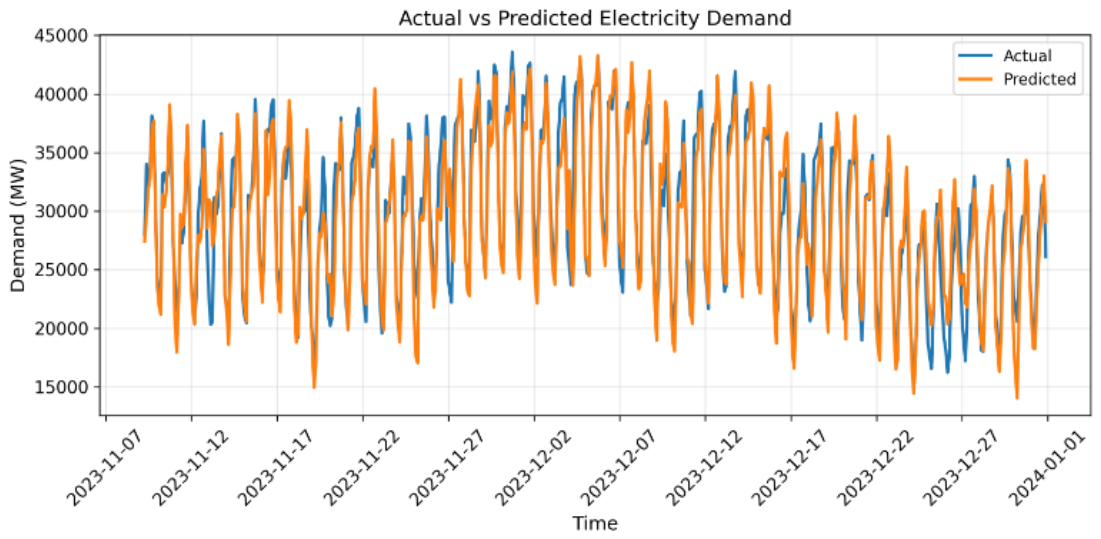
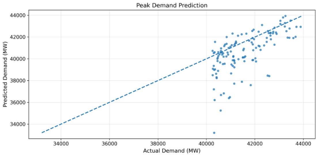
Figure 2 illustrates the comparison between actual demand $D_t$ and predicted demand ${\widehat{D}}_t$. The model captures overall demand structure effectively, including diurnal cycles and medium-term trends. To further assess model behaviour under critical operating conditions, Figure 3 presents prediction performance during high-demand periods. The model captures peak demand trends but exhibits deviations during extreme spikes. These deviations arise from the stochastic and low-frequency nature of such events, which are underrepresented in the training data and, therefore difficult to generalise.

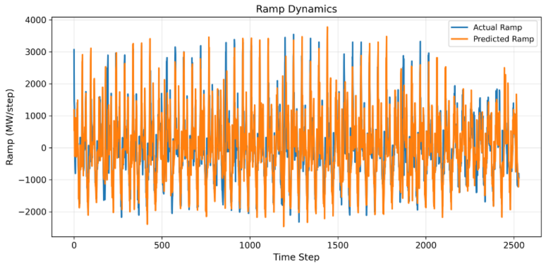
Ramp dynamics are analysed in Figure 4, where the temporal evolution of true and predicted demand gradients is compared. The model captures general ramp behaviour but shows reduced accuracy during abrupt transitions. These results indicate that while the model effectively learns underlying demand patterns, rapid transitions remain challenging due to their stochastic nature.

7.1. Error Characteristics and Robustness

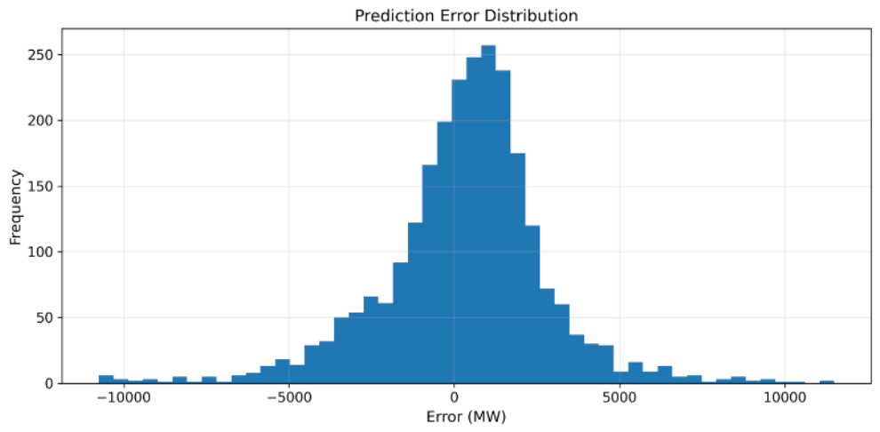
The distribution of prediction errors is analysed to assess model robustness. Figure 5 shows the histogram of residual errors. The error distribution is centred around zero with moderate dispersion, indicating that the model is largely unbiased. However, heavier tails suggest occasional large deviations associated with extreme demand conditions.

7.2. Grid Stress Modelling Performance

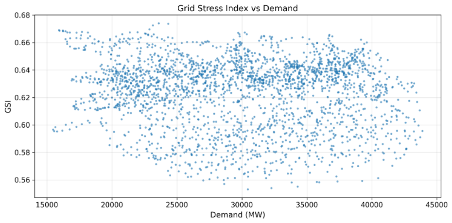
The effectiveness of the grid stress modelling component is evaluated by analysing the relationship between electricity demand and the predicted Grid Stress Index (GSI). Figure 6 illustrates the relationship between demand and predicted GSI values. The results show that the GSI tracks demand-driven stress patterns effectively. Periods of elevated demand correspond to higher stress levels, confirming that the model translates demand dynamics into meaningful operational indicators.

The effectiveness of the adaptive control module is evaluated by comparing system behaviour before and after mitigation. The results are summarised in

Table 2. Operational impact of adaptive mitigation.

Metric	Before Control	After Control
Peak Demand (MW)	43,946.33	41,586.24
Peak Reduction (%)	–	5.37
Max Ramp (MW/step)	3776.00	3772.82
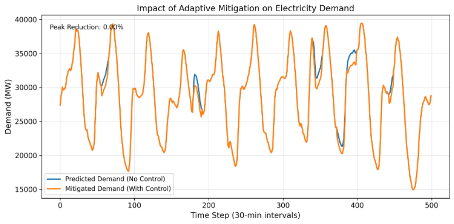
Ramp Reduction (MW/step)	–	3.18

. The adaptive mitigation strategy achieves a peak demand reduction of approximately 5.37%, demonstrating effective suppression of high-demand events and improved operational resilience. However, the impact on ramp dynamics remains limited, with only marginal reduction observed in maximum ramp rates. This indicates that the current control formulation is primarily optimised for peak shaving rather than temporal smoothing.

Furthermore, the observed increase in demand variability after mitigation suggests that aggressive peak reduction can introduce secondary fluctuations in the demand profile. This highlights an inherent trade-off between peak suppression and temporal stability. While peak reduction improves reserve margins and reduces system stress, insufficient coordination with ramp-aware mechanisms may lead to short-term variability. These results suggest that effective grid control requires multi-objective optimisation that jointly considers peak demand, ramp dynamics, and system stability. The current rule-based strategy provides a baseline implementation, but more advanced approaches such as optimisation-based control or reinforcement learning may be required to fully balance these competing objectives.

Figure 7 illustrates the effect of mitigation on the demand trajectory. These results highlight an inherent trade-off in grid control strategies. While peak demand reduction improves reserve margins and reduces system stress, it may also introduce variability if not coordinated with ramp-aware mechanisms.

Recent studies have demonstrated that grid flexibility can be further enhanced through integrated energy management approaches combining battery storage, hydrogen storage, ancillary services, and dynamic pricing mechanisms. In particular, synergistic coordination between electrical and hydrogen storage systems has shown potential for congestion management and resilience enhancement [39,40]. The proposed framework adopts a simplified battery and demand-response strategy to establish the operational feasibility of integrating forecasting, stress assessment, and mitigation. Future work will investigate multi-vector flexibility resources and optimisation-based scheduling strategies.

8. Conclusions

This study presented a hybrid deep learning framework for smart grid stress prediction and adaptive mitigation under extreme weather conditions. The proposed approach integrates demand forecasting, grid stress modelling, and adaptive control within a unified predictive–control architecture.

The results demonstrate that the model achieves stable predictive performance under real-world conditions, capturing key demand characteristics including peak behaviour and ramp dynamics. The Grid Stress Index provides a meaningful abstraction of system conditions by translating demand patterns into operational risk indicators.

The adaptive mitigation module delivers measurable operational benefits. From a practical grid operations perspective, the framework enables operators to move beyond passive forecasting by directly linking demand prediction to stress assessment and mitigation. This capability supports reserve planning, peak demand management, and proactive deployment of flexibility resources during weather-driven stress events. Simulation results show that peak demand can be reduced by approximately 5.37%, demonstrating the effectiveness of integrating predictive insights with control actions. However, limited improvement in ramp dynamics and increased variability highlight trade-offs in the current control formulation. A key implication of this work is that forecasting accuracy alone is insufficient for modern grid operation. Greater value is achieved through the integration of prediction, stress assessment, and control, enabling proactive rather than reactive system management.

A limitation of this study is that the model is trained on a single national-scale dataset, which may limit generalisability across different grid topologies and regulatory environments. In addition, the Grid Stress Index relies on fixed weighting parameters, and the control strategy is rule-based rather than optimisation-driven. These limitations highlight opportunities for future work in cross-system validation, adaptive stress modelling, and optimisation-based control. Future work will focus on integrating optimisation-based or reinforcement learning control strategies and validating the framework across multiple grid environments. From a systems perspective, the results demonstrate that embedding predictive models within a control-oriented framework significantly enhances their practical utility in real-world grid operation. The proposed framework provides a scalable pathway for integrating forecasting, stress assessment, and mitigation within existing energy management systems, supporting proactive grid operation under increasing weather-driven demand variability.