An Optimization Method for Data Aggregators and Smart Meters in Smart Grids

Abstract

In this paper a new mathematical optimization model is proposed to optimize the number of data aggregators in smart grids and assign each smart meter to at least one data aggregator. The model is based on a Set-Covering Problem, which aims to find the minimum number of sets that cover all elements. In the case of smart grids, these elements will be the smart meters. We used a branch–bound algorithm for the new optimization model to solve several instances considering different smart grid scenarios. In the scenarios, real-world parameters were used for a lot of smart meters (which ranged from 15 to 900, with output powers of 23 and 30 dBm used in the theoretical analysis), data aggregator costs, dispersions, maximum budget, and signal propagation losses. The tests reached the best values for the objective function with small, medium and large-scale instances in low computational times. Theoretical analysis was used to evaluate the signal received from data aggregators, indicating that they can receive information with a high-quality signal.The proposed model provides insights for stakeholders involved and can aid in smart grid implementation. In addition, it can offer a blueprint for engineers to optimize data flow within hierarchical grid structures with smart meters and data aggregators.

1. Introduction

The challenge for researchers and engineers is to decrease the losses caused in the electric power distribution in traditional grids, mainly in the final stage of the distribution of electricity. Efficient energy distribution through the use of state-of-the-art electronics and smart grids is the solution, according to [1]. Beyond that, the use of renewable resources to generate electricity is one alternative that incorporates consumer participation in the energy generation process.

Another point is that providing consumer feedback on consumption in real time through smart meters and using electric vehicle batteries to store and distribute energy to homes can be another solution for smart grids. From another point of view, smart grids are a natural advancement when addressing the topic of smart cities, as they are part of the concept of the Internet of Things [2].

The distribution of data aggregators throughout the electrical network makes them responsible for measuring, detecting faults, and acting as a bridge between the Smart Grid Control Center (SGCC) and smart meters. Data from smart meters can be stored for a specific period of time and sent to data aggregators. The communication between aggregators and meters is bidirectional, in which the data aggregators receive data from smart meters or send commands to the smart meters.

Data aggregators collect a wide variety of information from consumer endpoints, including granular measurements such as voltage, current, and grid frequency to monitor stability. The data aggregators process this information, transforming massive volumes of raw data into manageable, actionable insights using techniques such as averaging individual meter readings over specific intervals (e.g., 15 or 30 min). The data aggregators use a technique like compressed data aggregation, and sparse basis transforms are used to reduce communication overhead while maintaining high data fidelity. The aggregated data of the data aggregators is transmitted to SGCC to ensure the stability and efficiency of the power system using transmission methods. In this case, data are typically sent via secure bidirectional communication channels such as fiber optic, WiMAX, or 4 G/5 G cellular networks.

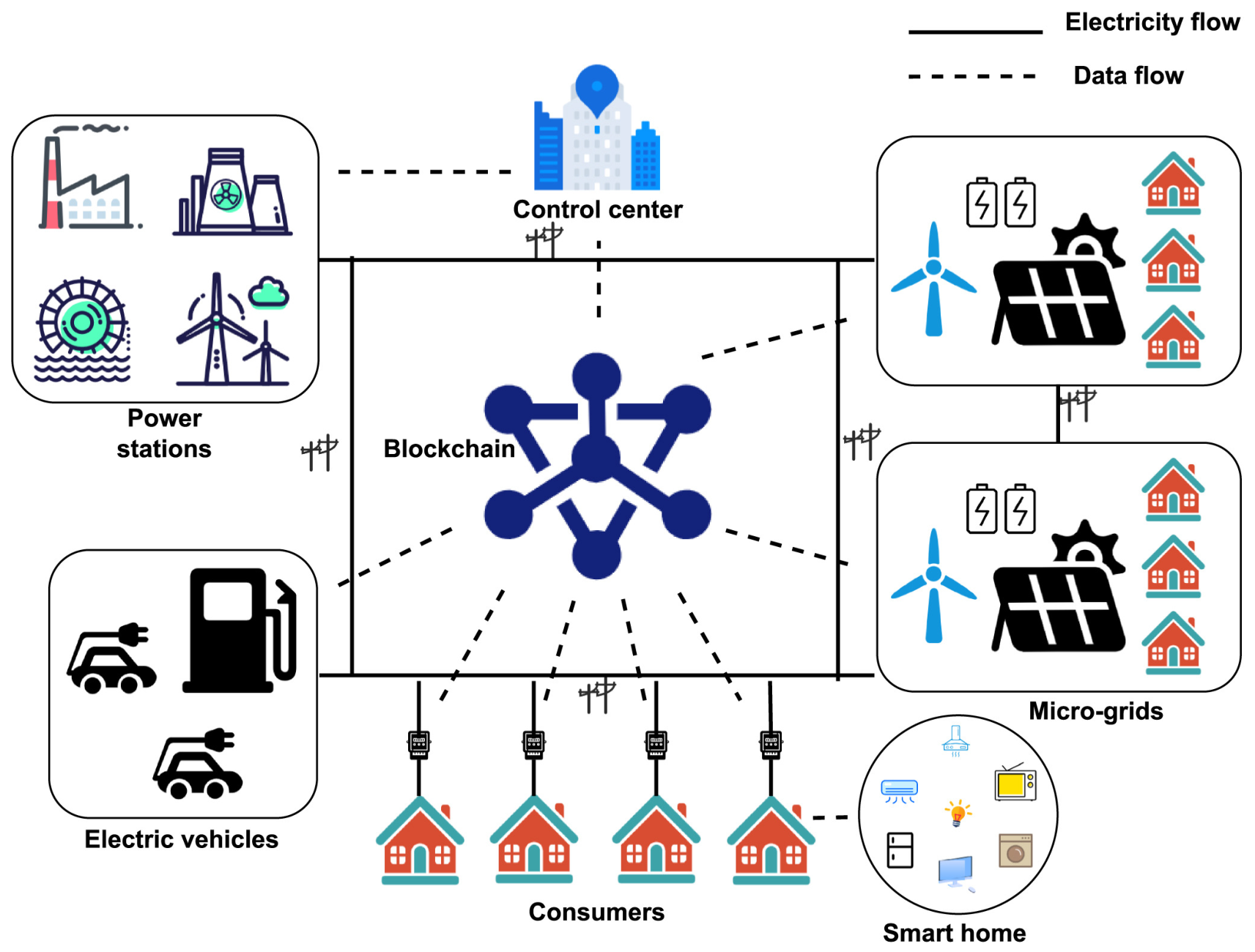
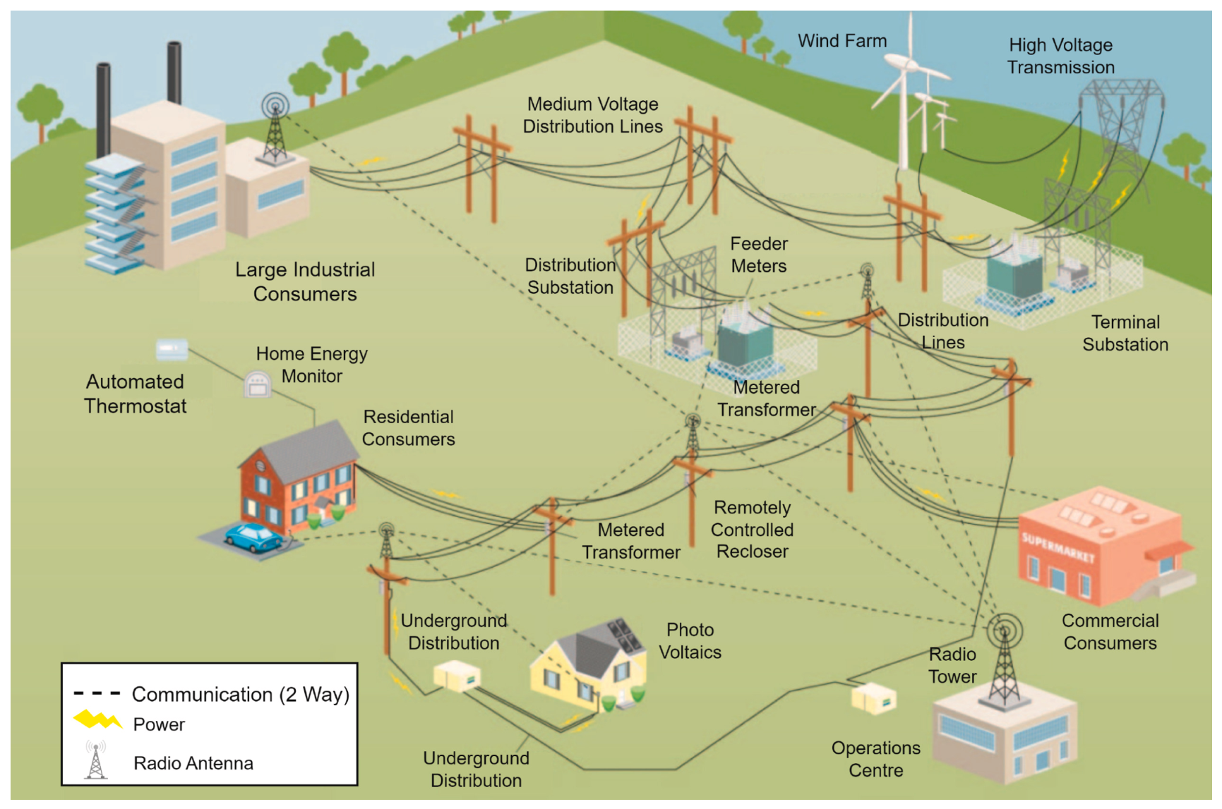
Bidirectional communication also occurs between the aggregators and the SGCC. The SGCC uses data from data aggregators to bill suppliers and pay generators correctly based on actual energy flow. Additionally, SGCC requests ancillary services (like frequency regulation or ramp rate control) from the aggregator’s fleet of assets using real-time data on frequency and voltage. Finally, the SGCC is located in the electricity concessionaire in which it stores consumer data and monitors and manages the entire smart grid, as shown in Figure 1.

Direct communication between a SGCC and millions of individual smart meters is considered infeasible due to several technical, economic, and security-related justifications. In addition, when a large number of smart meters transmit data at the same time, network congestion or collision will occur and even delay the entire system [4]. Many smart meters use low-power wireless technologies, such as ZigBee or Power Line Communication, which have a limited transmission range, often <100 m. Thus, smart meters cannot reach a distant SGCC without intermediate relay points. Moreover, the cost of establishing a dedicated Wide Area Network (WAN) for each individual meter is prohibitively high. Consequently, by using data aggregators, utilities can utilize lower-priced local networks for the last mile and exclusively invest in high-speed, long-range links for a smaller number of data aggregators. Furthermore, the number of entry points for cyberattacks is exponentially increased by direct connections to millions of meters. Data aggregators are responsible for protecting data by sanitizing and authenticating it before it is sent to the core grid infrastructure. Lastly, using raw, high-resolution usage data can reveal sensitive consumer habits such as when people are at home or what appliances they are using. Data aggregators employ privacy-preserving technology to provide grid operators with anonymized or aggregated data, protecting individual identities [5]. In this sense, the use of data aggregators is of vital importance.

In a smart grid, smart meters can store energy consumption data for each consumer. The authors of [6] claimed the following: by using smart meters, electric utilities and customers can communicate in a two-way manner, improving the efficiency of system operation and control; smart meter installations worldwide will reach over 900 million; fine-grained electricity consumption data is generated by smart meters widely deployed, which provides a wealth of information about the electricity consumption behaviors of electric customers; the power industry’s deregulation has the potential to provide valuable insights for electric utilities and customers to reduce energy costs through the analysis of smart meter data; and smart meter data analytics can aid in promoting renewable generation consumption and balancing the system through demand response as a result of the penetration of distributed energy resources. The data from smart meters will be sent periodically to at least one aggregator.

In [7], the authors demonstrate that choosing the most suitable positions for data aggregators is a challenging task, particularly in large cities with thousands of meters. Moreover, according to [7], network technologies, sensors, and electrical devices can use the information exchanged to provide interoperability, which is one of the main features of smart grids. Figure 2 shows an infrastructure of smart grid interoperability. In general, optimization problems take into account technological constraints to achieve optimal allocation of strategies over time, reduce economic costs, and minimize the overall loss [8]. For example, ref. [9] used the Traveling Salesman Problem to solve a routing problem for the established logistics operation of a commercial company.

Already in [10], the objective of the paper was to develop an algorithm based on k-Nearest Neighbors to allocate smart meters and data aggregators in a smart grid. Paper [10] proposed an optimization problem that located the data aggregators on smart meters to minimize installation and dispersion costs. Thus, as a consequence, the transmission and delay costs were also minimized.

According to [11], a smart grid has a set of smart meters and a set of data aggregators, generally located on top of communicating utility poles. These data aggregators communicate over wireless links. In addition, a smart grid also contains an advanced metering infrastructure (AMI), and Meter Data System Management (MDSM), which can collect the data measured by the smart meters.

The AMI is considered a key component of smart electricity grids, integrating software and hardware components, meter data management systems, monitoring systems, and information and control systems [12].

In this paper, an optimization problem was presented to locate and assign data aggregators to smart meters, the Optimization of Data Aggregators and Smart Meters (ODASM) in smart grids.

The work presents applications for smart grids that can contribute to demand side management, smart meters, and AMI. Beyond that, this paper can have a positive impact on modeling and design optimization methodology in smart grids. The optimization problem proposed in this paper is different from [13,14,15] considering the dispersion between data aggregators. In addition, it ensures that each meter is assigned to at least one aggregator within the specified radius.

Besides the works of [13,14,15], other relevant studies were included in the research. Specifically, refs. [16,17] provided foundational insights to refine the proposed optimization model, while ref. [18] contributed to defining the maximum distance between smart meters and data aggregators to ensure communication quality. Furthermore, signal propagation was investigated based on the works of [19,20,21,22,23,24]. Finally, the branch-and-bound method was implemented according to the definitions and frameworks established by [25,26,27]. The main contributions of the paper are:

• The problem of optimization with data aggregators and smart meters was formulated in smart grids in a binary integer nonlinear programming problem, which is different from the model in [15] which is a mixed-integer optimization problem. In addition, the proposed model differs from [15] because in the model of [15], every smart meter sends its data exactly to one data aggregator. In the proposed model, a smart meter can send data to more than one data aggregator. This last proposal is more flexible due to the situation of breaking a data aggregator. In this case, a smart meter can send another data aggregator. A smart meter will send data to at least one data aggregator according to the coverage matrix and the optimization algorithm. Initially, the coverage matrix assigns smart meters to data aggregators based on the maximum signal propagation distance. Upon implementing the proposed optimization algorithm, the smart meters are reallocated to at least one data aggregator to minimize the total number of devices (data aggregators) required to maintain full coverage.
• The ODASM problem optimizes five types of cost: installation, transmission, delay cost, dispersion, and a maximum budget to purchase the data aggregators.
• The proposed optimization problem finds the best location for aggregators and smart meters in wireless communication networks (without wired communication networks), which is easier to maintain and update circuits, scalability, and network security. Ref. [14] used an optimization problem to find the best location for data aggregators in hybrid wireless and wired communication networks, including fiber optic and WiMAX.
• The mathematical optimization problem proposed in this paper does not need calibration of the algorithm parameters because it uses an exact algorithm to solve the proposed model. This contrasts with the work of [10], where the algorithm of the authors needs calibration in the parameters of the kNN algorithm. Moreover, the kNN algorithm reached good solutions for k small values and the kNN algorithm stagnated for k large values.
• The mathematical optimization model proposed introduces a maximum budget to purchase the data aggregators in the model of [16], which also considered the dispersions among the data aggregators.
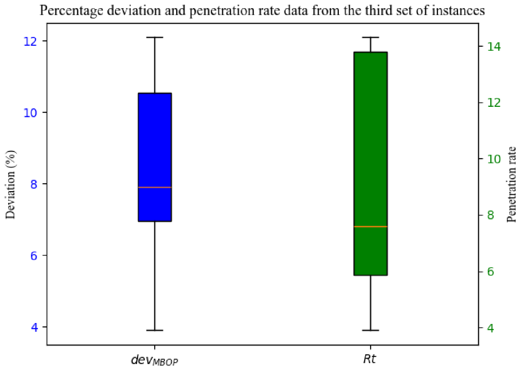
• To the best of available knowledge, three new metrics were introduced to validate the proposed methodology: the percentage deviation between the maximum budget and the global optimal cost; the penetration rate to evaluate current data aggregators already implemented in the smart grid that can fit the increasing number of smart meters due to consumer growth; and the maximum distance that data aggregators operate effectively within the range of acceptable signal to optimal signal strength. All these metrics will be redefined in the Section 4.
• Moreover, this paper proposes a new mathematical optimization model that results in improved performance compared to existing approaches, as the framework supports smart grid deployment by offering engineers a roadmap for data flow management. In addition, the new model helps to build hierarchical grid structures with smart meters and data aggregators, enabling utilities to achieve cost reductions and operational efficiency without compromising sustainability goals.

In summary, this study provides significant contributions to the literature regarding smart grid infrastructure optimization. Unlike the formulations proposed in [13,14,15], the optimization framework developed herein explicitly addresses the spatial dispersion among data aggregators while ensuring that each smart meter is assigned to at least one aggregator within a designated communication radius. The mathematical model was refined based on the foundational concepts established by [16,17]. To guarantee communication reliability, the maximum distance between smart meters and data aggregators was bounded according to [18], with signal propagation characteristics derived from the comprehensive studies in [19,20,21,22,23,24].

Furthermore, the optimization problem focuses exclusively on wireless communication networks, offering superior scalability, simplified circuit maintenance, and enhanced network security compared to hybrid architectures. For instance, while ref. [14] optimized aggregator placement using a combination of wired fiber optics and wireless WiMAX technologies, the purely wireless approach proposed here minimizes physical deployment constraints. Additionally, by employing an exact branch-and-bound algorithmic framework derived from [25,26,27], the proposed model yields exact solutions without requiring heuristic parameter tuning. This represents a major advantage over metaheuristic or data-driven approaches, such as the kNN-based algorithm in [10], which requires sensitive parameter calibration and suffers from performance stagnation at higher k values. Finally, this work extends the model from [16] by incorporating a realistic maximum budget constraint for aggregator procurement while preserving the analysis of aggregator dispersion.

The paper is structured as follows: Section 2 presents a mathematical optimization model and Section 3 the evaluation of signal propagation loss. In Section 4, materials and methods are presented. In Section 5 the results are described, and in Section 6 the discussion is presented. In the last section, the conclusions are outlined, as well as future work.

2. Mathematical Optimization Model

The proposed mathematical optimization model adds to the Set-Covering Problem (SCP) formulation described in [17]. It introduces a maximum budget, to purchase the data aggregators by the power distribution utilities and dispersion constraints, according to the model of [16]. This model is called MDSCP (Maximum budget Dispersion Set-Covering Problem). The dispersion constraints among the data aggregators are also factored into the set-covering problem to decrease redundancies and minimize the costs of delays between data packets, resulting in an optimal transmission.

The MDSCP is $\mathrm{NP}$-hard because it can be reduced to the SCP. The SCP is formally defined as follows: given a set of m elements of $M=\{1,\dots ,m\}$ and a collection of n subsets $N=\{S_j\subseteq M$, with $1\le j\le n\}$, with non-negative costs, a collection of subsets $X\subseteq N$ is a cover of M if the following holds: ${\bigcup }_{S_j\in X}{S}_j=M$. Then X is an optimal cover of M without any redundant subset in X; i.e., X will not cover M if any subset is removed from X. The SCP goal is to find a minimal cost cover X of M.

For the data aggregator allocation problem in a smart grid, the elements to be covered are the smart meters. A smart meter-made cluster should be covered by at least one candidate aggregator (where each has a cost of $c_j$), where X is composed of clusters of all allocated aggregators.

In this paper, it was assumed one-hop communication between smart meters and data aggregators according to [16], i.e., a single signal path from the smart meter to the aggregator. The MDSCP model is formulated as a binary integer nonlinear programming problem as follows:

$$minz={\displaystyle \sum _{j=1}^n}{c}_j·x_j,j=1,2,3,\dots ,n$$

(1)

subject to:

$${\displaystyle \sum _{j=1}^n}{a}_{ij}·x_j\ge 1,i=1,2,3,\dots ,m$$

(2)

$$r{x}_j·x_k\le dis{t}_{jk},r>0,\forall j,k,\in N$$

(3)

$${\displaystyle \sum _{j=1}^n}{c}_j·x_j\le MAX,j=1,2,3,\dots ,n$$

(4)

$$x_j\in \{0,1\},j=1,2,3,\dots ,n$$

(5)

where the decision variable $x_j=1$ if the subset $S_j$ belongs to cover X and $x_j=0$ otherwise; r is the minimum distance between two allocated aggregators; and $dis{t}_{jk}$ is the distance between the candidate data aggregator j and the candidate data aggregator k. In this paper, the Euclidean distance was applied to $dis{t}_{jk}$, which will be described below in the Section 4. Lastly, the coefficient $a_{ij}$ is equivalent to 1, if element $i\in S_j$ subset, and 0 otherwise. The matrix $A_{m\times n}$ is called the coverage matrix. In the coverage matrix, each row represents an element (smart meter) to be covered by the data aggregators, and each column represents a subset.

The objective function, Equation (1), minimizes the total cost to assign candidate data aggregators to smart meters. Note that there are several types of data aggregator in the real world, each with different costs. In the literature, these are simplified as a single cost $c_j=C$, for all $j=\{1,\dots ,n\}$, where C is a constant value. In this paper, different costs for candidate data aggregators are introduced based on channel capacity requirements. More details about the cost of data aggregators are provided in the Section 4.

Constraint (2) ensures that every smart meter must be covered by at least one aggregator. Constraint (3) ensures that the data aggregators have a minimum distance between them. The purpose of constraint (3) is to ensure that the aggregators are not in close proximity. These constraints allow different smart meters to be served by different aggregators.

Constraint (3) decrease redundancies, preventing delays between data packets. For radio communication between a smart meter and a data aggregator to take place, a maximum distance ($md$) between these two devices is required. This means that the distance between a smart meter and the data aggregators must be less than or equal to the transmission range of the smart meter. Consequently, it will result in a reduction in transmission and delay costs. 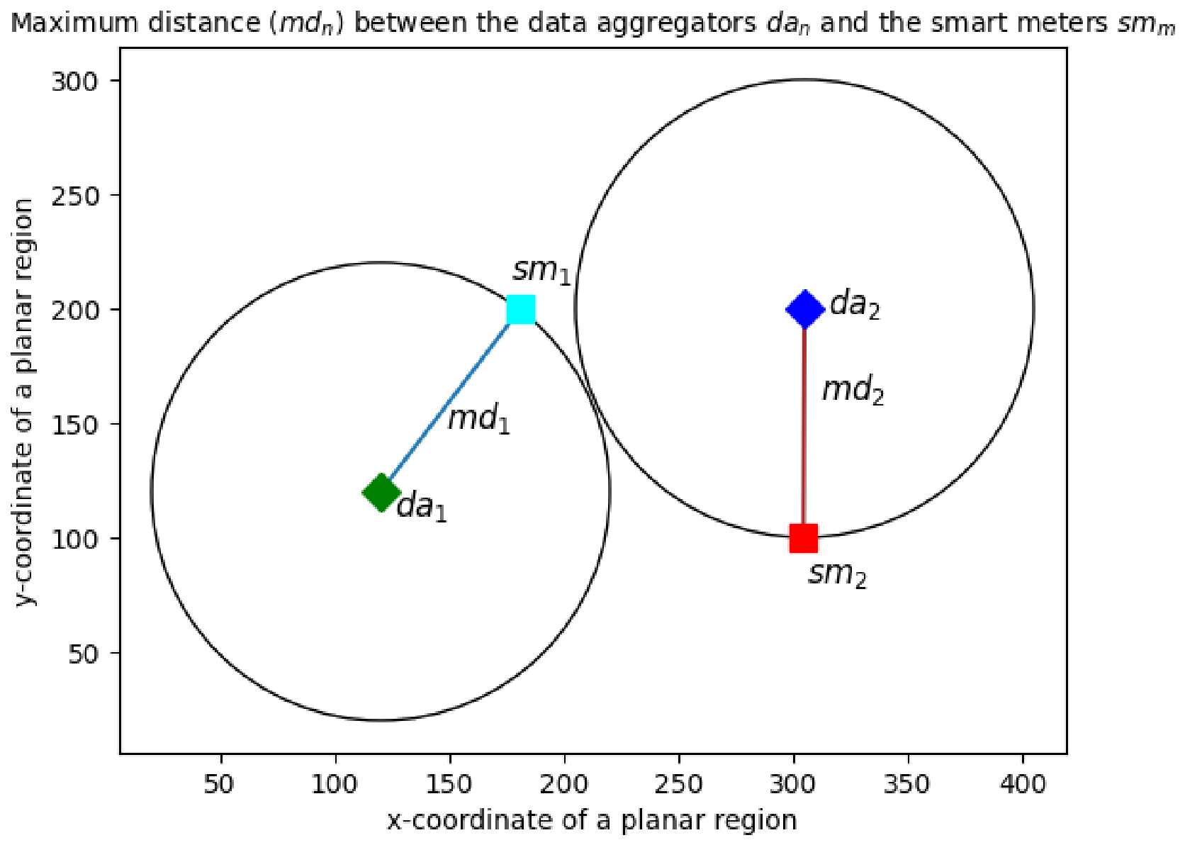Figure 3 shows the range of wireless signal communication radius ($md$) from two data aggregators, $d{a}_1$ and $d{a}_2$, ($j=1,2$), to two smart meters, $s{m}_1$ and $s{m}_2$, ($l=1,2$). In Figure 3 the maximum distance ($m{d}_1$) is equal to ($m{d}_2$) for the transmission radius range.

Therefore, to reduce the redundancy of the data aggregators, each must be at a minimum radial distance (r) from the others ($r\ge md$). According to [18], the value of $md$ was set equal to 100 m. Thus, it is set $r=100$ in constraints (3). Set $dis{t}_{jk}$ as the distance between the data aggregator j and the data aggregator k, for all $j,k\in N$.

The delay cost is modeled using a maximum distance ($md$) equal to 100 m in the proposed mathematical optimization model. Thus, the model optimizes the network topology by imposing this maximum distance to assign each smart meter to a data aggregator, thus reducing latency and communication overhead. The maximum distance ($md$) will be evaluated in the Section 3, and details of the network topology are provided in Section 4.

Signal propagation loss serves as an evaluation metric within the framework and is integrated indirectly into the proposed mathematical optimization model. Although it plays a secondary role in the primary decision-making process using constraint (3), it remains essential to account for delay costs and ensure low latency.

Constraint (4) considers a maximum budget ($MAX$) to purchase data aggregators by electricity utilities. The integrality constraints are described in (5) with the integer variables in the MDSCP model equal to 0 or 1, which represent the decision variables. The non-linear constraint (3) will be replaced by linear constraints to transform the proposed mathematical optimization model into an integer programming problem. This transformation ensures that the problem remains compatible with the standard branch-and-bound algorithm without affecting the optimal solution or the feasible region.

Although the original formulation is non-linear, linearization was performed to render the problem tractable for the branch-and-bound algorithm. Evaluating the minimum distances between aggregators is only mathematically meaningful if both are selected within the smart grid framework; hence, this condition holds only when the binary variables are set to 1. Mathematically, both formulations $rxj·xk\le dis{t}_{jk}$ and $2r\le (x_j+x_k)·dis{t}_{jk}$ are equivalent when $x_j$ = 1 and $x_k$ = 1, leading to $r\le dis{t}_{jk}$, in both formulations. A mathematical linearization technique was used for $rxj·xk\le dis{t}_{jk}$, and the strategy is described in Lemma 1.

Lemma 1.

Nonlinear constraints $rxj·xk\le dis{t}_{jk}$ can be expressed as linear constraints $2r\le (x_j+x_k)·dis{t}_{jk}$.

Proof of Lemma 1.

The proof demonstration is given as follows:

1.

Let ($x_j+x_k{)}^2$ = ${x_j}^2+{x_k}^2+2x_j·x_k$, where $x_j$ is equal 0 or 1; $x_k$ is also equal 0 or 1.

2.

In this sense, ${x_j}^2$ can be written as $x_j$ and ${x_k}^2$ as $x_k$.

3.

Observe that the maximum value of ($x_j+x_k{)}^2$ is equal to 4.

4.

Thus, 2$x_j·x_k\le 4/(x_j+x_k)$ and $x_j·x_k\le 2/(x_j+x_k)$.

5.

For $r{x}_j·x_k\le dis{t}_{jk}$ to be valid, $x_j$ = 1 and $x_k$ = 1.

6.

Consequently, $2r/(x_j+x_k)\le dis{t}_{jk}$ and regrouping for $2r\le (x_j+x_k)·dis{t}_{jk}$.

7.

Thus, it is possible to observe that the formulation $2r\le (x_j+x_k)·dis{t}_{jk}$ acts as a linear constraint.

   □

In the context of smart grids, channels of the data aggregators serve as the primary infrastructure for conveying energy metrics from smart meters to utility centers. The performance of these pathways is governed by predefined bandwidth slots and bitrates, which facilitate the streamlined processing and compression of metering data.

The costs of the data aggregators enforce the capacity limits of each data aggregator j, ensuring that the number of channels assigned ($n{a}_j$) does not exceed the number of maximum channels of each data aggregator ($n{m}_j$) for signals received from the surrounding smart meters.

Equation (6) defines the capacity limits for each selected data aggregator j (where the decision variable $x_j=1$, according to constraints (5)). In this regard, power flow analysis is integrated into the model indirectly to prevent data aggregators from becoming bottlenecks or underutilized, thus ensuring effective load balancing. It should be mentioned that the model minimizes the costs associated with the data aggregators required to cover a specific set of smart meters. In addition, the costs of the data aggregators are proportional to the number of channels that correspond to the capacity.

$$n{a}_j·x_j\le n{m}_j,x_j\in \left\{1\right\},j=1,2,3,\dots ,n$$

(6)

3. Evaluation of Signal Propagation Loss

An investigation of the theoretical analysis of the propagation of the signal path is conducted to analyze the performance of the communication system between smart meters and data aggregators using the proposed model in this paper. The strength of the signal decreases as electromagnetic waves travel from a transmitter to a receiver due to propagation loss in wireless communication. Factors such as distance, absorption, reflection, and scattering by obstacles cause propagation loss.

The ability to design wireless systems is crucial because it directly affects the coverage area and signal quality. In this sense, an evaluation will be performed based on the maximum distance ($md$ = 100 m) between a smart meter and a data aggregator according to [18] for good communication quality. Values accessible in the literature are utilized, such as: [13,15,19,20,21,22,23,24].

Thus, in the theoretical analysis, the path loss is evaluated, which is the loss of power of a radio frequency signal propagating through environments. The propagation loss is emphasized in [15] and the expected path loss over distance $d_{lj}$ is $PL\left(d_{lj}\right)$ as stated below:

$$PL{\left(d_{lj}\right)}_{dB}=PL{\left(d_0\right)}_{db}+10{\alpha }_{k}lo{g}_{10}\left(d_{lj}\right)-10{\alpha }_{k}lo{g}_{10}\left(d_0\right)$$

(7)

$$PL{\left(d_0\right)}_{dB}=20lo{g}_{10}(4\pi d_0{f}_k/c)$$

(8)

where

• l—the index of the starting device of the data link, which is a smart meter;
• j—the index of the ending devices of the data link, which is a data aggregator;
• $d_{lj}$—the distance from a smart meter l to a data aggregator j;
• $PL\left(d_0\right)$—the loss of signal propagation at the reference distance $d_0$, given as follows;
• ${\alpha }_k$—path loss exponent, it indicates the speed at which the signal power decreases with distance;
• $d_0$—the reference distance;
• $f_k$—the transmission frequency;
• c—the speed of light.

Paper [21] shows that $PL\left(d_0\right)$ is the path loss in a predetermined distance $d_0$ and $d_{lj}>d_0$, with $d_0$ = 10 m. As shown in [23] residential meters commonly use radio frequencies (f) equal to 169 MHz or 868 MHz, while GSM/GPRS is used for longer distances. Secondly, in [23], these data from a number of smart meters that make up the radio frequency communication network are collected by data aggregators, in a specific range. The radio frequency is beneficial for smart meters due to its low power consumption and optimal signal penetration capacity in buildings. In addition, there is a selection of data aggregators that can cover up to 1 km in a populated environment and 10 km without any urban obstacles.

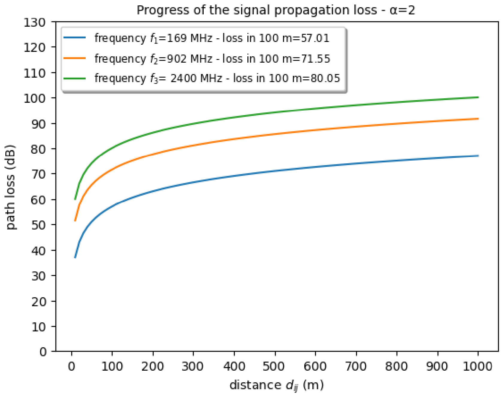
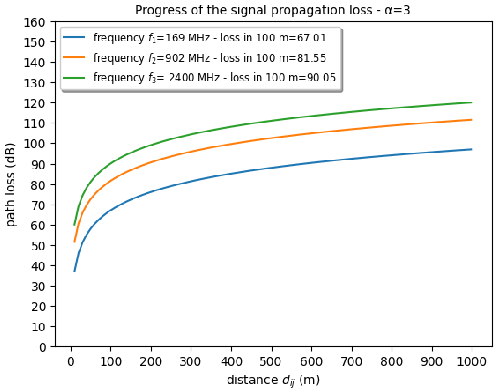
The power output of a smart meter can be around 1 W in the 902 MHz band, with much lower levels in the 2.4 GHz band. Using radio frequency communication, a data aggregator receives less power than the transmitted power of a smart meter. The received power influences the quality of the communication link and the amount of data in the aggregator can be received and processed successfully due to the distance to the transmitter and the radio environment. A connection can require a signal, around −75 dBm or −70 dBm, for the power of the received signal in a data aggregator in wireless networks.

However, in [20], the power specification of a data aggregator in its received signal is equal to −100 dBm, with the radius of smart meter communication being less than 0.93 km using the frequency of 2.4 GHz in a WLAN (Wireless Local Area Network). In this case, the maximum path loss presented was 123 dB.

Moreover, in [20], it was pointed out that a smart meter has transmission power of 0.2 W (23.0 dBm). In [13], the authors used a transmission power of smart meters with 0.1 W (20.0 dBm).

The literature provides classifications for the receiving power of signals on wireless receptors such as data aggregators. It can be adapted from [28] as follows: the signal value around −30 dBm (exceptional signal), the close signal value of −50 dBm (optimal signal), between −50 dBm and −70 dBm (reasonable signal), greater than −70 dBm and lower than −80 dBm (acceptable signal), and between −80 dBm and −90 dBm (very weak signal, with risk of disconnection).

In smart grids the smart meters are able to send data to the data aggregator for monitoring and billing systems using the 6LoWPAN (IPv6 over Low-Power Wireless Personal Area Networks), which is a low-power wireless technology. According to [24], the 6LoWPAN uses two frequency bands: worldwide between 2400 MHz and 2483.5 MHz, and North America, between 902 MHz and 929 MHz. Its range is 10 to 200 m.

In

Table 1. Standard values for ${\alpha }_k$, path loss exponent, adapted from [22].

Environments	$\mathit{\alpha }$	Description
Free space	2	This is the ideal scenario where radio waves propagate without any obstructions, similar to the Friis equation model.
Indoor	2–3	For propagation within a single floor of a building, the path loss exponent is generally higher than 2 due to signal reflections and obstructions.
Urban/Outdoor	2–4	In typical urban areas with buildings and other obstructions, the exponent falls within this range.
Dissipative	4–6	For very complex environments, such as those with significant vegetation or when considering full specular reflection from the earth’s surface (the flat earth model), alpha (${\alpha }_k$) can reach these higher values.
Particular	<2	In some cases, like a tunnel, the environment can act as a waveguide, resulting in a path loss exponent that is less than 2.

standard values for $\alpha$, which is the path loss exponent, are presented.

The smart meters send data to the data aggregators at a rate of minutes. Ref. [18] shows an example where data packets of a size of 2400 bytes are sent every 240 min from residential smart meters on the uplink and only 25 bytes are sent in the downlink over a period of 6 days. A smart meter can transmit from tens to thousands of bytes per transmission, depending on the data, protocol, and frequency, limited bandwidth, and path loss. The handling of a large number of a few kilobytes will be a challenge for communication architectures, and there is the possibility of packet loss [14]. The proposed model uses hierarchical grid structures with data aggregators and smart meters to implement communication architectures. Thus, it is important to evaluate the maximum distance between a smart meter and a data aggregator.

4. Materials and Methods

In this section, it will be described how the research was conducted from the choice of subject-matter until the findings. First, the methodology adopted was quantitative and exploratory because it involved exploring patterns in a range of numeric data [29] and bibliographic resources. These experiments were compared through the values of objective function, the computational times applied to a set of data, the penetration rates of data aggregators, and path loss of the propagation signals.

The following terms were then researched in various databases: optimization model, smart grids, smart meter, data aggregator, Set-Covering Problem, and power distribution systems. The chosen databases were Scielo, Scopus, Science Direct, and IEEE Xplore. Some papers were selected for the state-of-the-art technology of the research. Subsequently, the paper utilized the checklists as explained by [30].

Therefore, it is in compliance with the most effective practices of scientific communication. Next, several set-covering optimization models were analyzed and a mathematical optimization model was proposed for optimization of data aggregators and smart meters in smart grids. Because this selected model is a nonlinear programming problem, it was adjusted using a mathematical linearization technique.

After that, an exact method called branch–bound was applied to the proposed mathematical optimization model. This method used LINDO [31], a solver for optimization models. Finally, an analysis of computational tests was conducted considering the values in each instance of the objective function, computational time, penetration rate, and loss of signal propagation.

The primary steps of the branch and bound method (Algorithm 1) are described as follows, according to [25,26,27]:

Algorithm 1 Branch and bound method

1: Initialization—Formulate the problem by identifying the objective function and constraints according to the proposed mathematical optimization model. Solve a relaxed version of the problem (e.g., Linear Programming relaxation for integer problems) to find an initial feasible solution. The objective value of this solution is stored as the current best-known bound (the lower bound for minimization). The original problem is then added to the list of active sub-problems (nodes). 2: Node Selection—Select an unexplored sub-problem from the list of active nodes for processing. 3: Bounding—Calculate the bound for the optimal solution within the selected sub-problem. In integer programming, this bound is typically obtained via the Linear Programming relaxation of the sub-problem. If the sub-problem is found to be infeasible, it is pruned by infeasibility. 4: Pruning—Compare the bound of the current sub-problem with the current incumbent solution (the best feasible solution found so far). If the sub-problem’s bound indicates it cannot yield a solution better than the incumbent, the branch is pruned by bound and excluded from further consideration. 5: Branching—If a sub-problem is not pruned but its optimal relaxation solution remains fractional (for integer variables), divide the search space into two or more mutually exclusive sub-problems. For example, if a variable $x1=0.7$ must be an integer, create two new nodes with the added constraints $x1\le 0$ and $x1\ge 1$. These new sub-problems are then added to the list of active nodes. 6: Updating the Incumbent—If a feasible integer solution is found within a sub-problem and its objective value is superior to the current best-known solution, update the incumbent solution and the global bound accordingly. 7: Termination—Repeat Steps 2 through 6 until the list of active sub-problems is exhausted. The current incumbent solution is then verified as the global optimum for the original problem.

The method implicitly identifies all the possible solutions to the problem under consideration by storing sub-problems in a tree structure. The solution space is divided into smaller regions that can be solved recursively by unexplored nodes in the tree, and rules are employed to eliminate regions of the search space that may not be optimal. The best solution found in the search is retrieved once the entire tree has been explored. Secondly, in [26], three important components of the algorithm of the branch–bound method are the search strategy, branching strategy, and pruning rules. By default, the LINDO solver utilizes predefined strategies for its search, branching, and pruning algorithms.

Multiple scenarios composed of instances were tested using the MDSCP model for smart grids in a simulation way. The objective is to optimize performance without immediate real-world consequences by testing scenarios for results and analyzing data. Three sets of instances were generated: one small, another medium, and a last one that was large scale. To generate instances, according to the work of [11], communication devices were guaranteed to be distributed in the planar region in a way that covers at least one candidate data aggregator for each smart meter.

The installation cost structure of a data aggregator is primarily driven by three factors: the procurement of hardware components (Data Concentrator Units), the software overhead for aggregation (meter data management systems), and the labor and logistical expenses associated with the AMI setting.

Although total investment in data aggregators is influenced by various factors, including power connections and GPS modules, the number of measurement channels serves as the main cost driver, given that other hardware/software components remain consistent across units [32].

A data aggregator channel refers to the communication pathway used to transmit energy data such as voltage and current measurements from end-user devices to central utility systems [33]. These channels are defined by allocated bandwidth slots and transmission rates tied to sampling resolutions, typically at 15 min intervals [34], which impose specific computational overheads for data processing and compression [35].

In this paper, the analysis considered data aggregator units consisting of one voltage and two current measurement modules. These units are estimated to cost $40,000 each, with additional $4000 fees for every required current measurement channel beyond the base configuration [32]. Data aggregators often utilize multiple measurement modules to ensure reliability, prevent energy theft, and support complex grid operations such as bidirectional flow management.

In this paper, the installation cost of data aggregators is primarily driven by the number of measurement channels. Thus, the costs of the data aggregators applied in the proposed mathematical optimization model ranged from $100,000 to $152,000. Data aggregator costs do not account for the costs of data security (e.g., the use of encryption of the data sent by smart meters). Thus, the parameters used to the costs of the data aggregators in thousands of dollars used a discrete uniform distribution between 100 and 152, which corresponds to number of channels. The discrete uniform distribution emerged according to [36], with the random variable costs of the data aggregators ($c_j$), $j=1,\dots ,n$, taking on any integer value from 100 to 152 with equal probability.

In the context of smart grids, the allocation of smart meters to data aggregators is a complex optimization problem that balances communication efficiency with the physical realities of the electrical grid. To ensure reliability and cost-effectiveness in the distribution network, where each smart meter communicates directly with a single data aggregator, scenarios with three different sets of instances for the electrical grid were generated using a star topology that was integrated into the mathematical optimization model. A star topology is primarily a logical arrangement, though it is often supported by the physical reality of the hardware. In this topology, data travel in a single hop from the meter to the aggregator without being relayed by other meters along the way. The scenarios modeled on the electrical grid ensure that smart meters are grouped with data aggregators that share optimal geographical proximity, since the wireless signal propagates through the open air in all directions in the physical topology.

Network topology scenarios were not generated with high volatility (e.g., high penetration of solar photovoltaic or electric vehicle charging). Thus, the optimization problem can prioritize the assignment of smart meters to “closer” and “less burdened” data aggregators to allow for higher-frequency reporting.

In this sense, in a planar region, a random distribution of candidate data aggregators and smart meters was generated with three sets of instances with the following parameters:

(1)

In the first set, the number of data aggregators has a range between 4 and 15, and the smart meters between 15 and 40; the planar region is about 0.25 km² (with a length equal to 500 m per width of 500 m). These generated instances are called small-size instances.

(2)

In the second, the number of data aggregators was settled at 10, and smart meters have a range between 20 and 100; the planar region also is about 0.25 km² (with a length equal to 500 m per width of 500 m). These generated instances are called medium-size instances.

(3)

To evaluate the robustness of the proposed mathematical optimization model, a third set of instances was generated in a new planar region, here called large-scale instances. This new region was generated considering nine different zones. Each zone has similarity to the two sets of instances described above, which it has in the planar region of 0.25 km² (500 m × 500 m). However, the parameters of maximum budget, the number of data aggregators, and the number of smart meters were different.

The minimum radial distance (r) was considered equal to the three sets of instances. The second set was generated to evaluate the penetration rate of smart meters in a planned future horizon because the number of consumers may increase. In this sense, it was observed whether the number of candidate data aggregators is sufficient to meet the necessary number of smart meters in the future. A penetration rate is defined as: $Rt=m/nda$, where m is the number of smart meters and $nda$ is the number of data aggregators that were allocated;

For the third set of instances, the mathematical optimization problem was transformed into a decomposed problem where the original large-scale problem was reduced to several low-dimensional problems [37]. Then each low-dimensional problem was optimized, which was designed as a zone. In each zone of the planar region, an optimization problem with the objective function and its decision variables and constraints represents a group. Each group is guided by obtaining the optimal cost of the objective function and the number of data aggregators that were allocated. The values of each optimal objective function are added in each group, which will be the total cost of the objective function of the original large-scale problem. Furthermore, the total number of data aggregators allocated for the original large-scale problem will be determined by adding the values of the data aggregators allocated in each group. In this paper, the original large problem was called large-scale instances.

Despite the composition of the layout in the first set of instances and in the third, both were design for another purpose, the penetration rate was also evaluated for these two types of sets.

The value of r was set in 100, according to [18] to maintain the dispersion between the data aggregators. The calculation of distances $dis{t}_{jk}$ between the data aggregator j and k, for all $j,k\in N$ used the metric called the Euclidean distance [38]. The Euclidean distance (d) considers the distance between two points ($v_1$, $w_1$) and ($v_2$, $w_2$) in a two-dimensional plane as: d = $round\left(sqrt\right((v_2$ − $w_1{)}^2+(v_2$ − $w_1{)}^2\left)\right)$, where $sqrt$ is square root and $round$ is a rounded value.

Constraint (4) was added, as the $MAX$ can vary depending on the number of data aggregators spread throughout the planar region. In addition to [11], it was considered: (1) the bandwidth requirement of smart meters is identical for all; (2) smart grids in planar regions have a star topology (described above) in which smart meters and data aggregators are installed in urban scenarios without interference sources.

Now, the metrics used in this paper will be defined as follows.

1.

The percentage deviation $de{v}_{MBOP}$ between $MAX$ and the global optimal cost $OF$ is designed for $de{v}_{MBOP}=(MAX-OF)/MAX$;

2.

The penetration ratio ($Rt$) between the total number of smart meters m and the number of data aggregators allocated $nda$, given for $Rt=m/nda$;

3.

The maximum distance ($md$) means that the operation of the data aggregator maintains an acceptable-to-optimal signal strength range.

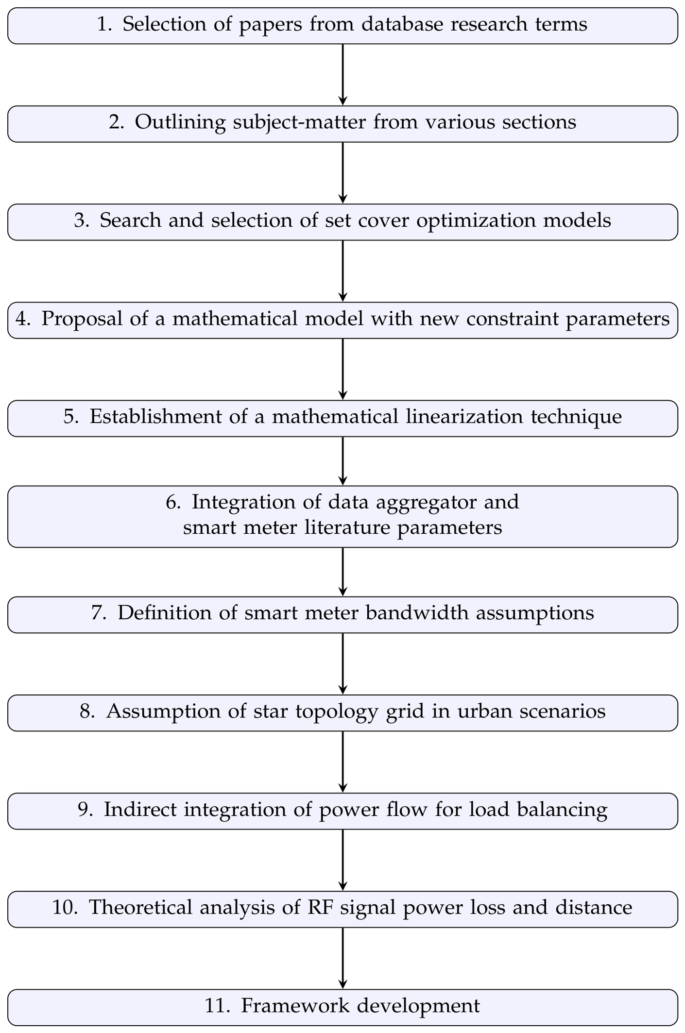
The proposed methodology is structured in two phases. The initial phase covers conceptual research and technical development, while the second phase presents a framework. This framework focuses on instance generation, integrates smart meter allocation to data aggregators accounting for distance constraints, obtains the coverage matrix, uses branch-and-bound optimization, and evaluates specific metrics using the proposed model to meet compliance requirements.

The initial phase is described as follows:

Step 1:

First, the research terms in the databases were examined to select several papers;

Step 2:

Second, written parts about subject-matter in various sections were outlined;

Step 3:

Third, the mathematical optimization models were searched for the cover of sets and one was selected;

Step 4:

Fourth, a mathematical optimization model was proposed with new parameters for the constraints of the previously selected model;

Step 5:

Fifth, on this occasion, a mathematical linearization technique was established;

Step 6:

After that, the work considered the parameters of the literature on data aggregators and smart meters for the proposed mathematical optimization model;

Step 7:

In due course, assumptions were made about the bandwidth requirements of smart meters;

Step 8:

Subsequently, the electrical grid in a star topology was assumed in urban scenarios without interference sources;

Step 9:

Then, the power flow analysis is integrated into the model indirectly to ensure load balancing and to prevent the received data of data aggregators from becoming bottlenecks;

Step 10:

Next, a theoretical analysis was carried out to evaluate the power loss of a radio frequency signal propagating through environments, taking into account the maximum distance.

Step 11:

In the last case, a framework was developed.

The second phase in the context of the proposed framework is presented as follows.

Step 1:

Following literature-based parameters and other parameters described above, it was developed an algorithm to generate simulated smart grid scenarios with star topologies. Three different instance sets were produced based on the aforementioned scenarios.

Step 2:

An instance is individually selected from the three previously defined sets in Step 1 for further analysis.

Step 3:

If the instance belongs to the first or second set, proceed to the Step 4; otherwise, go to Step 11.

Step 4:

The data from the instance selected, in Step 2, is stored with the spatial coordinates for both smart meters and candidate data aggregators.

Step 5:

The coverage matrix $A_{m\times n}$ using the selected instance, in Step 2, is constructed by assigning each l smart meter, $l=\{1,\dots ,m\}$, to the candidate data aggregators, subject to a maximum distance constraint ($md$). Each j data aggregator is a candidate data aggregator, being $j=\{1,\dots ,n\}$.

Step 6:

The distance $dis{t}_{jk}$ between the candidate data aggregator j and the candidate data aggregator k are calculated for all data aggregators ($\forall j,k\in N$) belonging to the selected instance in Step 2.

Step 7:

Equations (1)–(5) define the proposed mathematical optimization model for selected instance in Step 2.

Step 8:

The proposed model from Step 7 is solved to optimality using the LINDO solver, which employs a branch-and-bound method, described in Algorithm 1.

Step 9:

After identifying the allocated data aggregators in Step 8 by the method, their capacity limits are verified based on Equation (6).

Step 10:

Analytical results are reported considering the selected instance in Step 2: $gap$ of the cost of the objective function, computational time, $Rt$ penetration ratio, $de{v}_{MBOP}$ percentage deviation between maximum budget and global optimal cost, the allocated data aggregators, and optimal OF value. Go to Step 13.

Step 11:

In this case, the selected instance is a large-scale problem, it will be transformed into decomposed problems, reducing into various low-dimensional problems. Each low-dimensional problem is classified as small-to-medium instance and it will be solved to optimality using Steps (4)–(9). For each instance, the framework records the optimal OF value, the computational time, and the number of allocated data aggregators. Upon evaluating all low-dimensional problems, proceed to Step 12.

Step 12:

The results of the analysis from large-scale problem are summarized as follows: the total optimal cost of OF, $de{v}_{MBOP}$ percentage deviation between maximum budget and total optimal cost of OF, total computational time, total number of allocated data aggregators, and $Rt$ penetration ratio. Go to Step 13.

Step 13:

End of proposed framework.

In Figure 4 the methodological flow chart of the initial phase is shown.

Algorithm 2 outlines the optimization and evaluation procedure for all smart grid instances generated by the proposed framework.

Algorithm 2 Optimization and evaluation of smart grid instances

1:  procedure  InstanceExecution  2:      Generate simulated smart grid scenarios and three instance sets (Set 1, Set 2, and Set 3) based on literature parameters.  3:      while There are unprocessed instances. do  4:          Select an individual instance from the sets for analysis.  5:          if Instance belongs to Set 1 or Set 2 then  6:             Store spatial coordinates for smart meters and candidate data aggregators.  7:             Construct coverage matrix $A_{m\times n}$ based on distance constraint ($md$).  8:             Calculate distances $dis{t}_{jk}$ between all candidate data aggregators.  9:             Formulate the optimization model using Equations (1)–(5). 10:            Solve to optimality using LINDO solver (Algorithm 1). 11:            Verify capacity compliance for allocated aggregators via Equation (6). 12:            Report results ($gap$, time, $Rt$, $de{v}_{MBOP}$, allocated aggregators, and OF value). 13:         else 14:            Decompose the large-scale instance into various low-dimensional sub-problems. 15:            for each low-dimensional problem do 16:                Apply Steps 6 to 11 to solve to optimality. 17:                Record OF value, computational time, and number of allocated aggregators. 18:            end for 19:            Summarize results (total cost, $de{v}_{MBOP}$, total time, $Rt$, and allocated aggregators). 20:         end if 21:     end while 22:     return End of Instance Execution. 23: end procedure

The proposed methodology will be validated through a set of metrics described as follows: first, the difference ($gap$) between the cost of the objective function and the global optimum cost in the proposed optimization model; second, the percentage deviation between the maximum budget and the global optimal cost; third, the penetration rate determined by evaluating the capacity to gradually increase the number of data aggregators, i.e., fit the growing number of smart meters as a result of increased consumers; fourth, the results of the theoretical analysis of path loss in signal propagation about the maximum distance that data aggregators operate effectively; and lastly, the compliance with the capacity of the data aggregators, according to Equation (6).

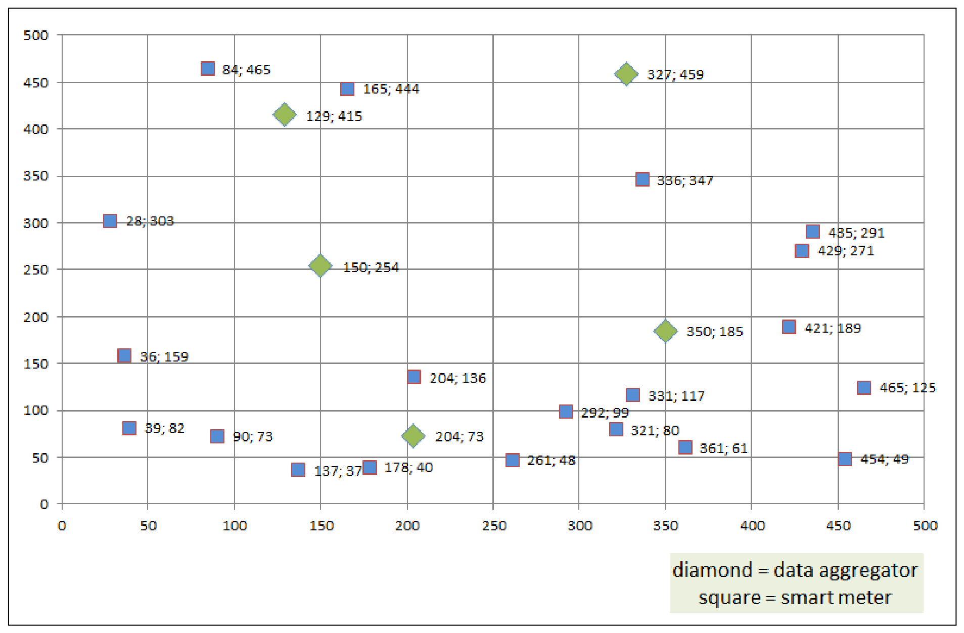
A partial application of the framework is demonstrated with the help of Figure 5, a small-size instance of a planar region. In Figure 5 all parameters are shown: 5 data aggregators, 20 smart meters, area of 0.25 km² (500 m × 500 m), maximum budget equal to 510 thousand dollars, minimum radial distance (r) equal to 100 m, and costs of data aggregators between 100 and 152 thousand dollars.

For the small-size instance in Figure 5, the coverage matrix $A_{m\times n}$ is defined in

Table 2. Coverage matrix $A_{m\times n}$ for the small-size instance of Figure 5: m = 20 smart meters ($sm$) and n = 5 data aggregators ($da$).

da/sm	1	2	3	4	5
1	0	1	0	0	1
2	0	0	0	1	1
3	0	1	0	0	1
4	0	0	1	1	0
5	1	1	0	0	0
6	0	1	0	1	1
7	0	0	0	1	1
8	0	1	0	1	1
9	0	1	0	0	0
10	1	0	0	1	0
11	0	1	0	1	1
12	0	1	0	0	1
13	1	1	0	0	0
14	0	0	0	1	1
15	0	0	0	1	1
16	0	1	0	1	1
17	0	0	0	1	1
18	0	1	0	0	1
19	1	0	0	0	0
20	1	1	0	0	0

.

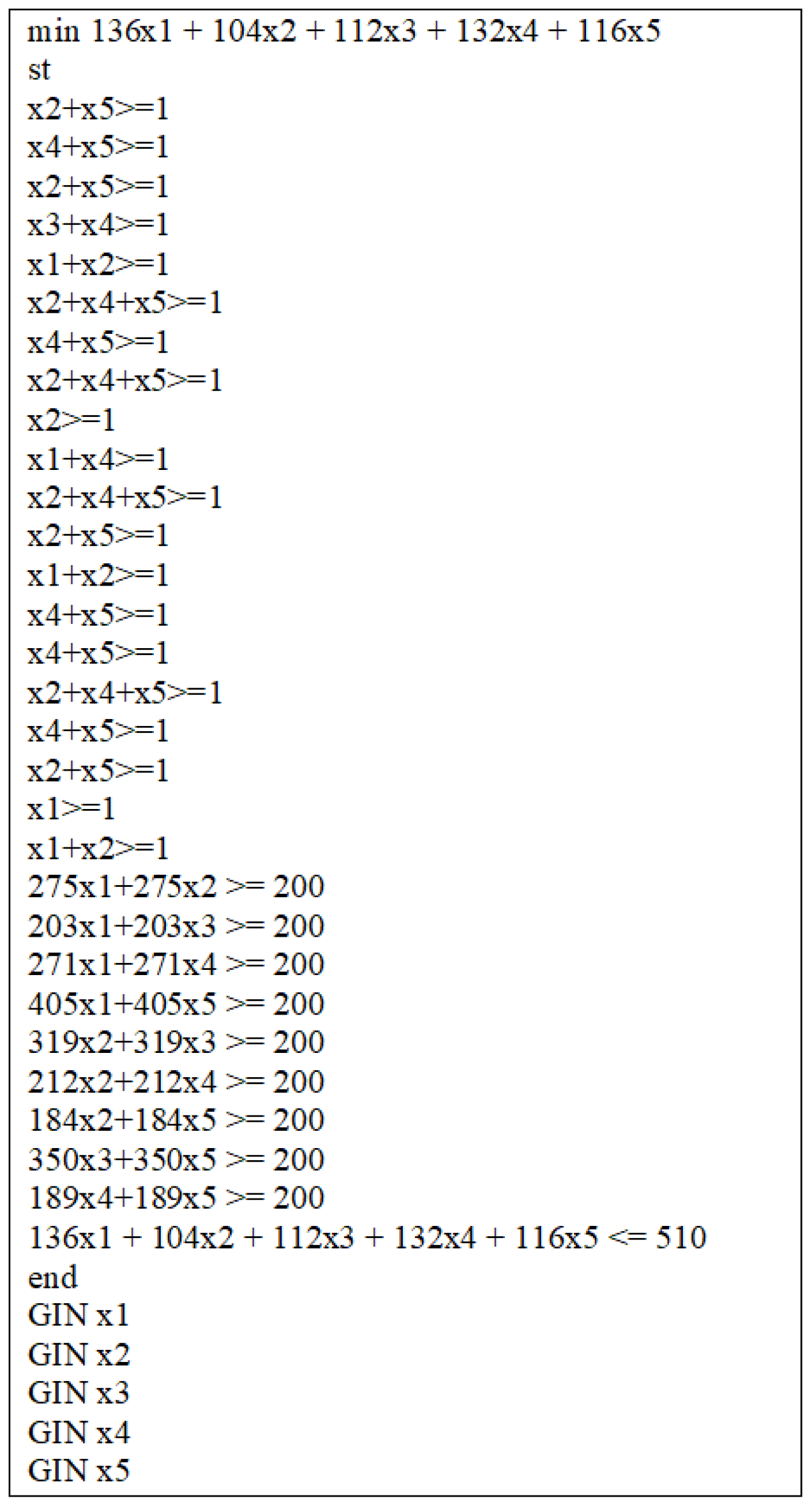
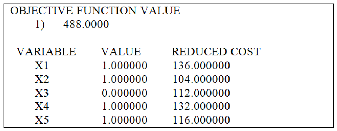
Figure 6 shows the mathematical optimization problem with information of instance described in Figure 5. However, the solution of the problem indicated in Figure 6 is shown in Figure 7. Figure 7 shows the data aggregators of numbers 1, 2, 3, 4, and 5 represented by variables $x_1,x_2,x_3,x_4,x_5$, respectively. In this case, all variables were set equal to 1, except $x_3$. The $OF$ was equal to 488 thousand dollars and the maximum budget was equal to 510 thousand dollars. In this sense, using a small-size instance as in Figure 5, an electricity utility will save 112 thousand dollars, which is the cost of the data aggregator of number 3 not selected.

The metrics proposed to evaluate the solution were as follows: the percentage deviation $de{v}_{MBOP}$ = 4.7%, the penetration ratio $Rt$ = 5, and the maximum distance $md$ = 100 m. Considering the small-size instance, in Figure 5, $OF$ reached the global optimum cost with $gap$ equal to 0, reaching the optimality. The compliance with the capacity of the data aggregators was maintained by ensuring that the channel allocation remained within the maximum limits specified for each device, according to Equation (6) shown in

Table 3. Compliance with data aggregator capacity for the small-size instance of Figure 5.

Data Aggregator	Number of Channels Assigned	Number of Maximum Channels
1	5	26
2	12	18
3	0	20
4	11	25
5	13	21

.

5. Results

In this section, the results reached from the proposed optimization model and the findings about signal propagation loss will be presented.

The computational results were reached with a computer as follows: Intel^® processor, Core™ i7, 2.20 GHz, RAM 8 GB, 64 bit operation system and 6 cores. It used LINDO solver release 6.1 as a branch–bound method. The computational times, using the solver, were very low when considering the generated instances according to the Section 4.

5.1. Results of Proposed Optimization Mathematical Model

The parameter of the first set of instances, the number of data aggregators was in the range between 4 and 15, and the number of smart meters between 15 and 40. In the second set of instances, the number of data aggregators was settled at 10, and the smart meters have a range between 20 and 100. In both sets, the minimum radial distance (r) was equal to 100 m, and the costs of the data aggregators were between 100 and 152 thousand dollars. The maximum budget was in the range between 600 and 1200 thousand dollars.

Taking note of the parameters of the third set of instances in a new planar region (large-scale instances), it was distributed in nine different zones. Each zone has similarity to the two sets of instances described above, which it has in the planar region of 0.25 km² (500 m × 500 m). The minimum radial distance (r) was established to be equal to the one mentioned earlier. However, there was a difference in the maximum budget parameters, in the number of data aggregators, and in the number of smart meters. More details can be observed in Table 7.

Table 4. Results of optimization problems for the first set of instances.

Instances	n	m	NR	MAX	OF	t (s)	ADG
scp4-15-100-152	4	15	22	600	560	<1	1, 2, 3, and 4
scp5-20-100-152	5	20	31	650	403	<1	2, 3, and 5
scp6-25-100-152	6	25	41	750	342	<1	1, 4, and 6
scp7-30-100-152	7	30	52	800	596	<1	2, 4, 5, 6, and 7
scp8-35-100-152	8	35	64	850	554	<1	1, 2, 4, 6, and 7
scp9-40-100-152	9	40	77	850	550	<1	1, 2, 3, 5, and 7
scp10-45-100-152	10	45	91	900	572	<1	1, 5, 6, 7, and 9
scp11-50-100-152	11	50	106	900	897	<1	1, 2, 4, 6, 7, 8, and 11
scp12-55-100-152	12	55	122	1000	997	<1	1, 2, 3, 5, 6, 8, 10, and 12
scp13-60-100-152	13	60	139	1000	854	<1	1, 2, 3, 5, 6, 8, and 10
scp14-35-100-152	14	35	127	1200	1165	<1	1, 2, 3, 4, 5, 6, 8, 12, and 14
scp15-40-100-152	15	40	146	1200	1126	<1	1, 5, 6, 7, 8, 9, 10, 12, and 13

presents the values of the modeled optimization problem for the first set of instances. In the first column are shown the instances, in the second the number of candidate data aggregators (n), in the third the number of smart meters (m), and in the fourth column the $NR$ (number of restrictions–lines of optimization problem). In the fifth column $MAX$ is shown, and in the sixth the value of $OF$, both in thousands of dollars. In the last columns are presented the computational time (t) in seconds and the allocated data aggregators ($ADG$), respectively.

The significance of the maximum capital constraint is exemplified by an instance selected from Table 4. Thus, in

Table 5. Result of an optimization problem for an instance of the first set.

Instances	n	m	NR	MAX	OF	t (s)	ADG
scp7-30-100-152	7	30	52	infinite	833	<1	1, 2, 3, 4, 5, 6, and 7

, it was observed, for example, in the instance scp7-30-100-152 that if the maximum budget is not considered, all variables $x_j$, with $j=1,\dots ,7$, would be settled equal 1, with all data aggregators being selected. Thus, the $OF$ was equal to 833, which being the formulation of the problem with $OF$ = min $133x_1+101x_2+104x_3+149x_4+131x_5+104x_6+111x_7$ and other constraints, according to the mathematical optimization model proposed, described above.

This maximum capital analysis can be extended to the other instances in Table 4; for clarity, Table 5 was made separately.

It was observed that $OF$ in Table 5 is greater than Table 4 for the scp7-30-100-152 instance. In this sense, the constraint for maximum budget aids the electricity utilities in reducing costs, while maintaining sustainability and improving the efficiency of system operation and control. In conclusion, the hypothesis is similar in other instances in Table 4 because the constraint related to the maximum budget introduces a cut in the polyhedron in the constraints of the proposed optimization problem.

It was observed that the costs of the objective function in Table 4 depend on the random prices of the data aggregators and the geographical positions distributed in the planar region of the smart meters and data aggregators. In general, the cost of the objective function increases in proportion to the increase in the number of smart meters and data aggregators. The data aggregators allocated varied between three and nine, as shown in Table 4.

The results in Figure 8 show the percentage deviation from the maximum budget and the penetration rate for the first set of instances, with the data on the axis x corresponding to $de{v}_{MBOP}$ in the first box and $Rt$ in the second. In the axis y on the left is the percentage deviation (%) of the maximum budget, and on the right the magnitude of penetration rates. Figure 8 shows the penetration rate $Rt$ that varied between 3.8 and 9.0 and $de{v}_{MBOP}$ in the range between 0.3% and 54.4%. The values of $de{v}_{MBOP}$ varied significantly considering these instances.

Table 6. Results of optimization problems for the second set of instances.

Instances	n	m	NR	MAX	OF	t (s)	ADG
scp10-20-100-152	10	20	66	650	577	<1	3, 5, 6, 8, and 9
scp10-25-100-152	10	25	71	800	640	<1	4, 5, 7, 8, and 10
scp10-30-100-152	10	30	76	800	642	<1	2, 4, 5, 7, and 9
scp10-35-100-152	10	35	81	800	787	<1	2, 4, 5, 7, 8, and 9
scp10-40-100-152	10	40	86	900	839	<1	1, 2, 3, 4, 5, 6, and 9
scp10-45-100-152	10	45	91	900	572	<1	1, 5, 6, 7, and 9
scp10-50-100-152	10	50	96	900	845	<1	1,2, 4, 5, 6, 7, and 9
scp10-55-100-152	10	55	101	900	748	<1	2, 5, 6, 7, 8, and 10
scp10-60-100-152	10	60	106	900	880	<1	2, 3, 4, 6, 7, 9, and 10
scp10-65-100-152	10	65	111	850	792	<1	1, 3, 4, 8, 9, and 10
scp10-70-100-152	10	70	116	850	843	<1	3, 5, 6, 7, 8, 9, and 10
scp10-75-100-152	10	75	121	850	766	<1	1, 2, 3, 5, 7, and 10
scp10-80-100-152	10	80	126	850	760	<1	1, 3, 4, 5, 6, and 9
scp10-85-100-152	10	85	131	850	750	<1	1, 4, 6, 7, 8, and 9
scp10-90-100-152	10	90	136	900	883	<1	1, 2, 3, 5, 6, 7, and 10
scp10-95-100-152	10	95	141	950	777	<1	2, 4, 6, 8, 9, and 10
scp10-100-100-152	10	100	146	1000	740	<1	1, 4, 5, 7, 8, and 10

presents the values of the optimization problems for the second set of instances. The descriptions of the columns in Table 6 are the same as those presented in Table 4. In Table 6, it is observed that the costs of the objective functions had light variation compared to Table 4 due to the fact that the number of aggregators was constant.

In both Table 4 and Table 6, the computational times were very small and less than one (1) second. In some instances, the maximum budget was tight in relation to the values of objective function; for example, in the instance scp11-50-100-152, the maximum budget was equal to 900 and the cost of the objective function equal to 897. Moreover, in the instance scp10-70-100-152, the maximum budget was equal to 850 and the cost of the objective function equal to 843.

Taking into account the penetration rate of smart meters in Table 6, it was observed that the number of candidate data aggregators (equal to 10) was sufficient for the number of smart meters in a range of 20 to 100. In this case, the data aggregators allocated varied between 5 and 7 as shown in Table 6. The number of data aggregators allocated did not vary significantly.

In Figure 9, the values of the percentage deviation from the maximum budget and the penetration rate are shown for the second set of instances. The penetration rate $Rt$ ranged between 4.0 and 16.7 and $de{v}_{MBOP}$ obtained a range between 1.6% and 36.4% (outlier), as shown in Figure 9.

Table 7. Results of optimization problems for the third set of instances.

Id	n	m	MAX	OF	${\mathit{dev}}_{\mathit{MBOP}}$ (%)	t (s)	nda	Rt
1	108	495	9000	8059	10.5	<1	65	7.6
2	117	540	9500	8841	6.9	<1	72	7.5
3	126	315	10,800	10,382	3.9	<1	81	3.9
4	135	360	11,500	10,698	7.0	2	86	4.2
5	90	810	7900	7062	10.6	<1	57	14.2
6	90	855	8550	7514	12.1	<1	60	14.3
7	90	900	8800	8106	7.9	<1	67	13.4

presents the values of the optimization problems for the third set of instances. In the first column are shown the $Id$ identifier of the instances, in the second the number of candidate data aggregators (n), in the third total number of smart meters (m), and in the fourth $MAX$. Moreover, in the fifth column is shown the $OF$, in the sixth the percentage deviation $de{v}_{MBOP}$ between $MAX$ and $OF$, and in the seventh the computational time (t) in seconds. In the last columns are presented the number of allocated data aggregators ($nda$) and the ratio $Rt$ between the total number of smart meters and the number of allocated data aggregators, respectively.

In Table 7 the smart meters ranged between 315 and 900 and the allocated data aggregators varied between 57 and 86. In addition, it was observed in Table 7 that when smart meters varied between 810 and 900, the number of allocated data aggregators ranged between 57 and 67. Therefore, considering the last case, the hierarchical architecture of the smart grid, proposed in this paper, proves its resilience by ensuring operational efficiency with minimal changes to data aggregators, effectively handling the increasing deployment of smart meters. Moreover, optimization in data flow within hierarchical grid structures with smart meters and data aggregators is facilitated.

In addition, it is observed in Table 7 that the ratio $Rt$ was in the range 3.9 to 14.3. The instance $Id$ of number 3 reached the lowest $de{v}_{MBOP}$ between the maximum budget and the cost of the objective function, equal to 3.9%, $de{v}_{MBOP}$ = (10,800 − 10,382)/10,800. Instance (Id = 6) reached the highest $de{v}_{MBOP}$ equal to 12.1%, $de{v}_{MBOP}$ = (8550 − 7514)/8550. Therefore, imposing maximum budget constraints is essential for optimizing data aggregators and smart meters within hierarchical smart grid architectures.

In Figure 10, all details about the percentage deviation and the penetration rate are shown for the third set of instances.

It highlights that the best integer solutions were reached for all instances in Table 4, Table 5, Table 6 and Table 7. Thus, the costs of the objective function ($OF$) of the proposed mathematical optimization model, shown in Table 4, Table 5, Table 6 and Table 7, reached the global optimum costs with the $gap$ equal to zero (0) for all instances. A branch–bound algorithm in the Lindo solver [31] was used for all instances.

The convergence of branch-and-bound algorithms is measured by the difference ($gap$) between the best integer solution (primal bound) and the best dual bound. When this difference reaches zero, the incumbent solution is proven to be the global optimum. Therefore, the algorithm proposed in this paper does not require comparison with heuristics or other methods as it eliminates the need for parameter calibration.

It was also highlighted that compliance with the capacity of the data aggregators was ensured for each device, according to Equation (6), for all instances shown in Table 4, Table 5, Table 6 and Table 7.

5.2. The Findings of Signal Propagation Loss

The assumption of maximum distance $md$ was evaluated to know if it is true for proposed optimization model and the computational results. In this sense, to evaluate the maximum distance ($md$ = 100 m) between a smart meter and a data aggregator, several scenarios were generated for values of $d_{ij}$, ${\alpha }_k$, and $f_k$ with $d_0$ = 10 m. The values of $md$ equal to 120 m and 140 m were also used to evaluate. In

Table 8. Numerical values to evaluate the path losses.

Parameter	Unity	Values
$d_0$	m	10
$f_k$	MHz	169, 902, 2400
${\alpha }_k$	-	[2–6]
$md$	m	100, 120, 140
output power of a smart meter	dBm	23, 30
input power of a data aggregator	dBm	[(−30)–(−90)]

, a summary of numerical values is presented to evaluate loss of signal propagation.

In Figure 11, it is observed that the path loss was 57.01 dB, 71.55 dB, and 80.05 dB in distance $md$ = 100 m for frequencies $f_i$, $i=1,2,3$, equal to 169 MHz, 902 MHz, and 2400 MHz, respectively. In this sense, $f_1$ and $f_2$ have a good signal quality, and $f_3$ is a lightly acceptable signal.

In Figure 12, the path losses in relation to the distance with $\alpha$ = 3 are shown. The propagation loss values were greater than the values presented in Figure 11. In $md$ = 100 m, the frequency $f_1$ = 169 MHz has a good signal quality. At frequencies $f_2$ = 902 MHz and $f_3$ = 2400 MHz, the signals were lightly acceptable.

In Figure 13 considering distance $md$ = 100 m and $\alpha$ = 4, the path loss was 77.01 dB, 91.55 dB, and 100.05 dB at frequencies 169 MHz, 902 MHz, and 2400 MHz, respectively. Thus, the conclusion is that the signal has a slight good quality at a frequency of 169 MHz, and it is lightly acceptable at other frequencies.

Figure 14 shows the signal propagation loss at several distances with variations of $\alpha$ at a frequency of 169 MHz. In this frequency, there is good quality of the signals considering the distances (100 m to 140 m) and $\alpha \le 4$.

Figure 15 also shows the signal propagation loss at several distances with variations of $\alpha$ at a frequency of 902 MHz. In this case, the quality of the signals is considered lightly acceptable with $\alpha \le 4$ in distances: 100 m to 140 m.

Again, Figure 16 shows the loss of signal propagation at several distances with variations of $\alpha$ at a frequency of 902 MHz. In this case, the quality of the signals is considered barely acceptable for distances (100 to 140 m) and $\alpha >2.5$. However, with $\alpha \le 2.5$, the quality of the signals is considered acceptable.

Figure 16 shows the path loss of the signal for the distances 100 m, 120 m, and 140 m, at a frequency of 2400 MHz. Signal propagation losses increase with higher values of $\alpha$.

Table 9. Path losses in $dB$ between transmitters (smart meters) and receptors (data aggregators).

OPT (dBm)	IPR (dBm)	f (MHz)	$\mathit{\alpha }$	PL (dB)
23	−34.01	169	2	57.01
23	−44.01	169	3	67.01
23	−54.01	169	4	77.01
30	−27.01	169	2	57.01
30	−37.01	169	3	67.01
30	−47.01	169	4	77.01
23	−48.55	902	2	71.55
23	−58.55	902	3	81.55
23	−68.55	902	4	91.55
30	−41.55	902	2	71.55
30	−51.55	902	3	81.55
30	−61.55	902	4	91.55
23	−57.05	2400	2	80.05
23	−67.05	2400	3	90.05
23	−77.05	2400	4	100.05
30	−50.05	2400	2	80.05
30	−60.05	2400	3	90.05
30	−70.05	2400	4	100.05

shows the path losses in dB between transmitters (smart meters) and receptors (data aggregators) considering several frequencies and parameters $\alpha$ according to Figure 11, Figure 12 and Figure 13 at a distance $md$ equal to 100 m. In Table 9, the first column shows the output power of the transmitter (OPT), in the second column the input power of the receptor (IPR), and in the third column the frequency (f). In the last columns the parameter $\alpha$ and the path loss (PL) are presented.

To evaluate the signal received from the data aggregators, two types of smart meters were considered, one with 23 dBm and another with 30 dBm. The power received by the data aggregators was between −27.01 dBm and −77.05 dBm. In this context, data aggregators can operate within a signal-to-noise ratio (SNR) that ranges from acceptable to optimal levels.

Now, considering Figure 14, Figure 15 and Figure 16 with $md$ equal to 120 m and 140 m, there was little variation in the loss of signal propagation. In conclusion, the results support the hypothesis that $md$ = 100 m is the maximum distance and suggest that it can be raised to 140 m.

5.3. Performance Evaluation for PMU Allocation: A Real-World Case Study

In the next step, the framework was applied to a case study of a specific allocation problem. A PMU (Phasor Measurement Unit), often referred to as a Synchrophasor, is defined as an advanced monitoring device that measures electrical quantities, such as voltage magnitude, current, frequency, and phase angle, in synchronized and real time [32]. This unit form a Wide-Area Measurement System (WAMS) transmitting data to Phasor Data Concentrators (PDCs) for real-time grid analysis. Standard PDCs typically support a maximum of 40 PMU streams.

In this sense, the proposed framework will be applied to the Optimal PMU Placement Problem (OPP) using the IEEE 33-bus radial distribution system (Figure 17). The network topology is mapped to a connectivity matrix to ensure the complete observability of the network while minimizing the number of installed PMUs [39]. Due to the radial nature of the test system, the traditional coverage matrix is replaced by a connectivity-based formulation to streamline the observability constraints.

The mathematical modeling of OPP for the IEEE 33-bus system is described as follows:

$$min{\displaystyle \sum _{i=1}^{33}}{c}_j·x_j$$

(9)

subject to:

$$A·X\ge b$$

(10)

where $x_j=1$ if a PMU is installed on bus j, and 0 otherwise. $\mathbf{A}$ is the binary connectivity matrix of order $33\times 33$ given by the constraints (10). $\mathbf{X}$ is the decision vector ${[x_1,x_2,\dots ,x_{33}]}^T$. $\mathbf{b}$ is a unit vector ${[1,1,\dots ,1]}^T$, which ensures that each bus is observed at least once. The objective function (Equation (9)) minimizes the number of PMUs. Note that the MDSCP can be reduced to the OPP.

The distance $dis{t}_{jk}$ between a candidate PMU j and a candidate PMU k, as well as the minimum distance r between two PMUs, was not considered because PMUs generally use optical fiber in communication. The costs $c_j$ for each PMU were assumed to be constant (equal to 1).

The connectivity matrix $A_{n\times n}$ defines which buses are observed by a PMU installed on the bus j. In this formulation, n represents the total number of buses. To ensure observability of the radial distribution system, the elements of the connectivity matrix are defined as:

$$a_{jk}=\left\{\begin{array}{cc}1,\hfill & \mathrm{if}j=k,(\mathrm{a}\mathrm{PMU}\mathrm{observes}\mathrm{its}\mathrm{own}\mathrm{bus})\hfill \\ 1,\hfill & \mathrm{if}\mathrm{buses}j\mathrm{and}k\mathrm{are}\mathrm{adjacent}\hfill \\ 0,\hfill & \mathrm{otherwise}\hfill \end{array}\right.$$

(11)

Example using Figure 17: let bus 2 be connected to bus 1 and to buses 3 and 19; the constraint will be: $x_1+x_2+x_3+x_{19}\ge 1$, according to the constraints (10). This means that bus 2 will be observed if there is a PMU on the bus itself (2) or on its neighbors (1, 3, or 19).

Zero injection buses (ZIBs) can be considered as buses without load or generation, depending on the network topology and desired redundancy. In this sense, by applying Kirchhoff’s Law to expand system observability, the total number of required PMUs can be reduced. Thus, the constraints ($f_i$) for each bus (i) with ZIB are modified in the OPP as follows:

$$f_i={\displaystyle \sum _{j=1}^{33}}{a}_{ij}·x_j+\sum _{k\in adj\left(i\right)}{z}_{ik}\ge 1,i=1,2,3,\dots ,n$$

(12)

where $z_{ik}$ is an auxiliary binary variable associated with the ZIB at bus k.

The performance of various PMU allocation methods and the proposed framework (with and without ZIB) using the IEEE 33-bus is summarized in

Table 10. Results of the PMU allocation approaches using the IEEE 33-bus.

PMUs	Number of PMUs	Number of ZIB (Buses)	Reference
2, 5, 8, 11, 14, 17, 21, 24, 27, 29, 32	11	0	Proposed Framework
3, 6, 9, 12, 15, 18, 20, 23, 28, 31	10	4 (1, 22, 25, 33)	Proposed Framework
2, 6, 9, 12, 16, 19, 21, 24, 27, 29, 32	11	0	[41] (using a algorithm)
2, 5, 8, 12, 16, 21, 24, 27, 30, 33	10	0	[41] (using integer programming)
2, 5, 8, 11, 14, 17, 21, 24, 27, 30, 33	11	0	[42]
2, 5, 8, 11, 14, 17, 21, 24, 29, 32	10	2 (6, 27)	[42]
2, 4, 8, 11, 14, 17, 21, 24, 26, 29, 32	11	0	[43]
2, 8, 11, 14, 17, 21, 24, 26, 29, 32	10	4 (5, 6, 13, 21)	[43]
2, 4, 8, 11, 14, 17, 21, 24, 26, 29, 32	11	0	[44] (using PSO)
2, 4, 8, 11, 14, 17, 21, 24, 26, 29, 32	11	0	[44] (using GWO)

. The majority of these approaches required 11 PMUs.

Several metrics proposed in this study were applied to the IEEE 33-bus instance, specifically the objective function cost gap (which achieved zero), the number of PMUs allocated (as detailed in Table 10), and the computational time. The computational processing time for the algorithm using the proposed framework is consistent with existing approaches, averaging around one second, rendering any efficiency gap statistically insignificant for practical smart grid applications.

To determine the optimal PMU configuration based on total installation costs, primarily driven by the number of channels, several test instances were generated. The impact of maximum budget constraints was also analyzed. For each configuration listed in

Table 11. Results of the instances with several configurations for IEEE 33-bus.

Configuration	PMUs	${\mathit{N}}^{\mathit{o}}$ of PMUs	OF	MAX	${\mathit{dev}}_{\mathit{MBOP}}$ (%)	${\mathit{gap}}_{\mathit{OF}}$ (%)
1	2, 5, 8, 11, 14, 17, 21, 24, 27, 30, 33	11	1438	1450	0.83	0
2	2, 5, 8, 11, 14, 17, 21, 24, 27, 30, 33	11	1323	1350	2.00	0
3	2, 5, 8, 11, 14, 17, 21, 24, 27, 29, 32	11	1332	1380	3.48	0
4	2, 5, 8, 11, 14, 17, 21, 24, 27, 30, 32	11	1368	1370	0.15	0
5	2, 4, 8, 11, 14, 17, 21, 24, 26, 29, 32	11	1265	1300	2.69	0
6	2, 4, 8, 11, 14, 17, 21, 24, 26, 29, 32	11	1370	1400	2.14	0
7	2, 4, 8, 11, 14, 17, 21, 24, 26, 29, 32	11	1339	1350	0.81	0
8	2, 5, 8, 11, 14, 17, 21, 24, 26, 29, 32	11	1403	1450	3.24	0
9	2, 5, 8, 11, 14, 17, 21, 24, 27, 30, 33	11	1350	1400	3.57	0
10	2, 4, 8, 11, 14, 17, 21, 24, 26, 29, 32	11	1427	1470	2.93	0

, PMU costs were uniformly distributed between $100,000 and $152,000, as described in the Section 4.

Table 11 presents the percentage deviation ($de{v}_{MBOP}$, sixth column), which was consistently narrowed in all instances. Furthermore, all solutions achieved optimality with a $ga{p}_{OF}$ of zero. The best optimal PMU configuration based on total installation costs was number 5 with $OF$ equal to $1,265,000.

6. Discussion

The smart grid is a way to transmit electrical power with reliability, management, and the incorporation of renewable energy into electric distribution systems. The mathematical optimization model proposed allocates data aggregators and smart meters that assist smart grids in interoperability, and it helps the advanced metering infrastructure. In this sense, this work contributes to the promotion of smart grids.

In the local region, EDP Brazil has installed 50,000 smart meters in the State of Espírito Santo and plans to surpass the 1 million mark by 2025 [45]. The main objective of these investments is to improve the electrical distribution system to facilitate the execution of the “Legal Framework for Micro and Mini Distributed Generation” in Brazil [46]. This investment is almost twice what was invested between 2016 and 2020. In addition, this investment has other objectives: improving the operations in the distribution electrical network, decreasing losses (compounding energy theft), and investing in digitalization and upgrades in customer services.

The paper formulated an optimization problem with data aggregators and smart meters in a nonlinear binary integer programming problem, which was different from the models in the literature. This model also differs from the literature because it optimizes transmission delay and dispersion (imposing a maximum distance to assign each smart meter to a data aggregator) and the maximum budget to purchase the data aggregators by electricity utilities. Because it uses an exact algorithm, the mathematical optimization problem proposed in this paper does not require calibration of the parameters of the method.

The proposed optimization problem found the best location for aggregators and smart meters in wireless communication networks. In this sense, solving an optimization problem supports maintenance and enables efficient updating of electrical and electronic circuits.

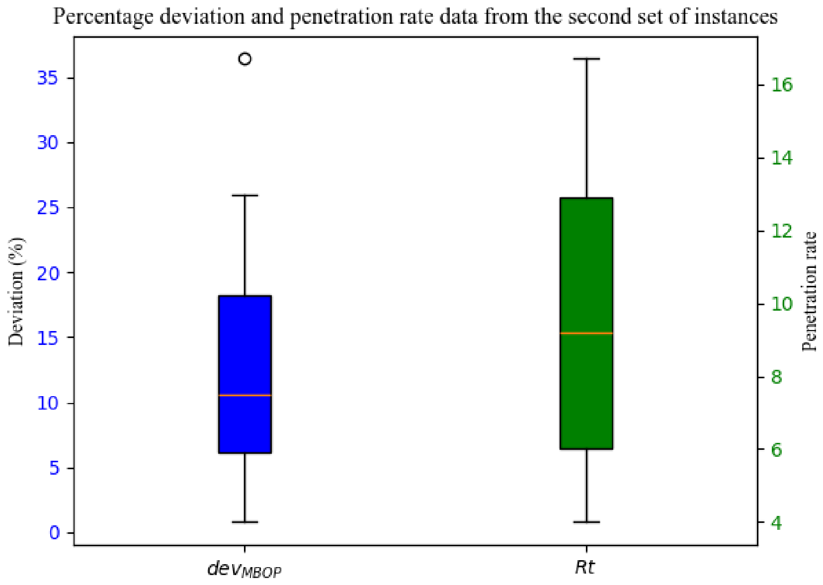
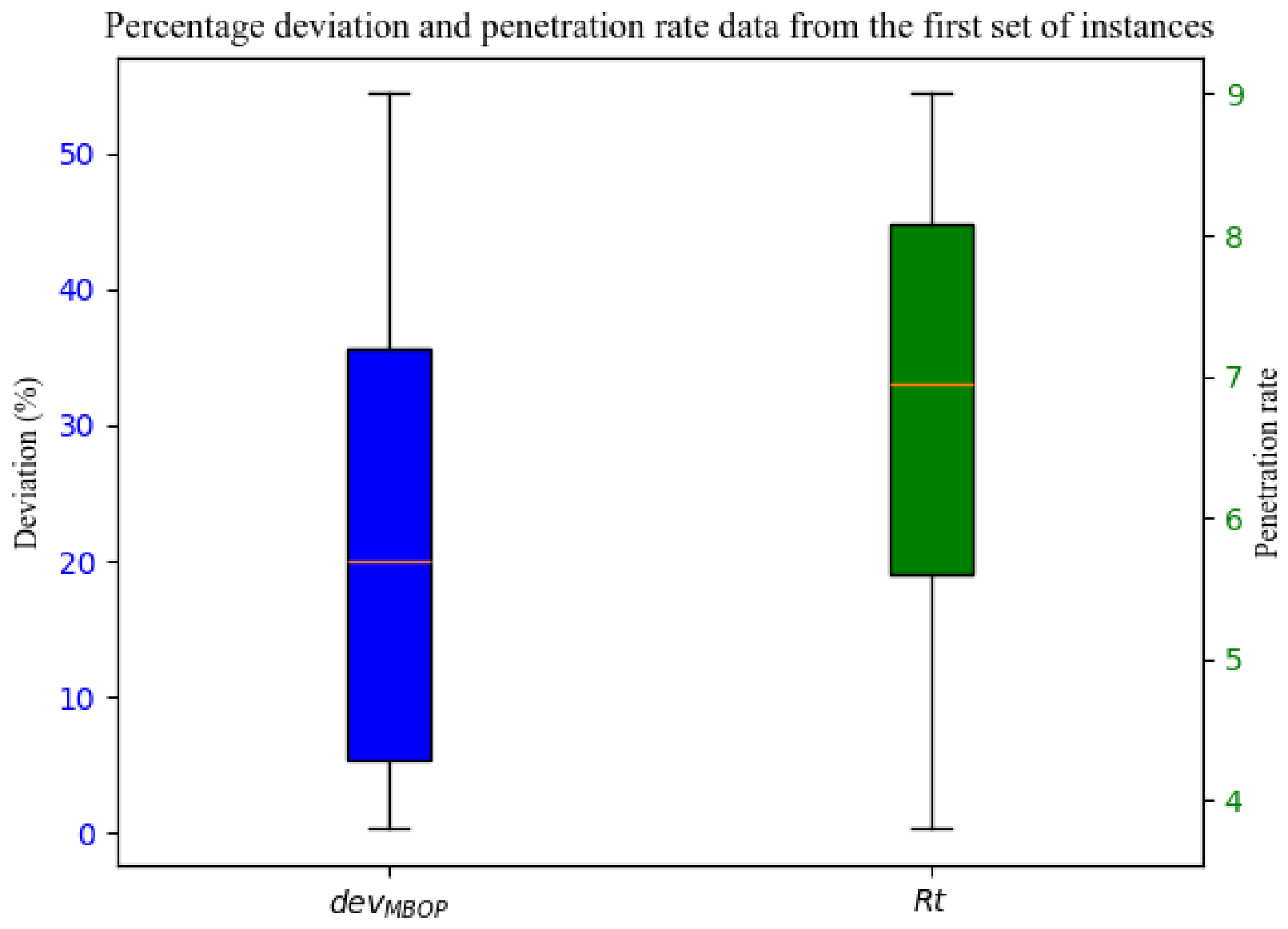
According to the computational results presented in this work, the smart meters had a ratio ($Rt$) with respect to the allocated data aggregators of 3.8 to 16.7. The $Rt$ is lower than the proportion presented in the paper of [11] that was between 28 and 36.25, without considering a maximum budget. Each data aggregator has several channels to receive data from smart meters, whose installation costs range from 100 to 152 thousand dollars. 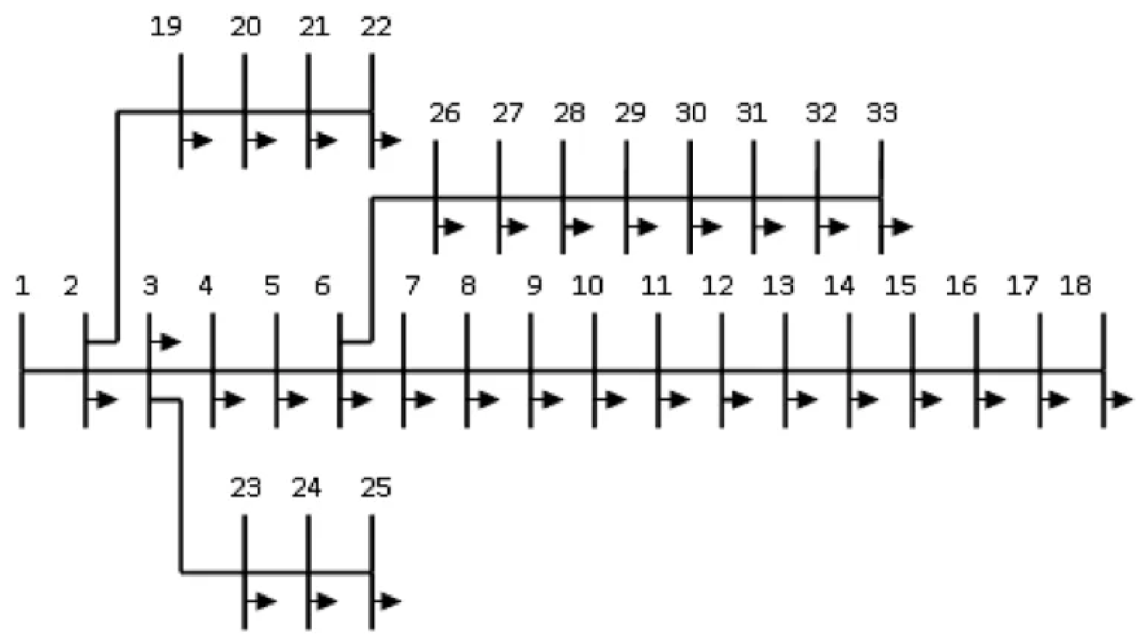Provided that $Rt$ was between 3.8 and 16.7, the constraints on the maximum budget cooperate with the costs of acquisition of data aggregators that will be acquired by the electricity utilities. Another point that can be highlighted is the computational times which were slightly shorter than 2 s for small-, medium-, and large-scale instances. The methodology was validated using the IEEE 33-bus radial distribution system, and the results were compared with existing literature.

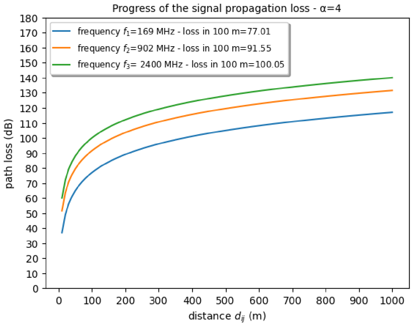
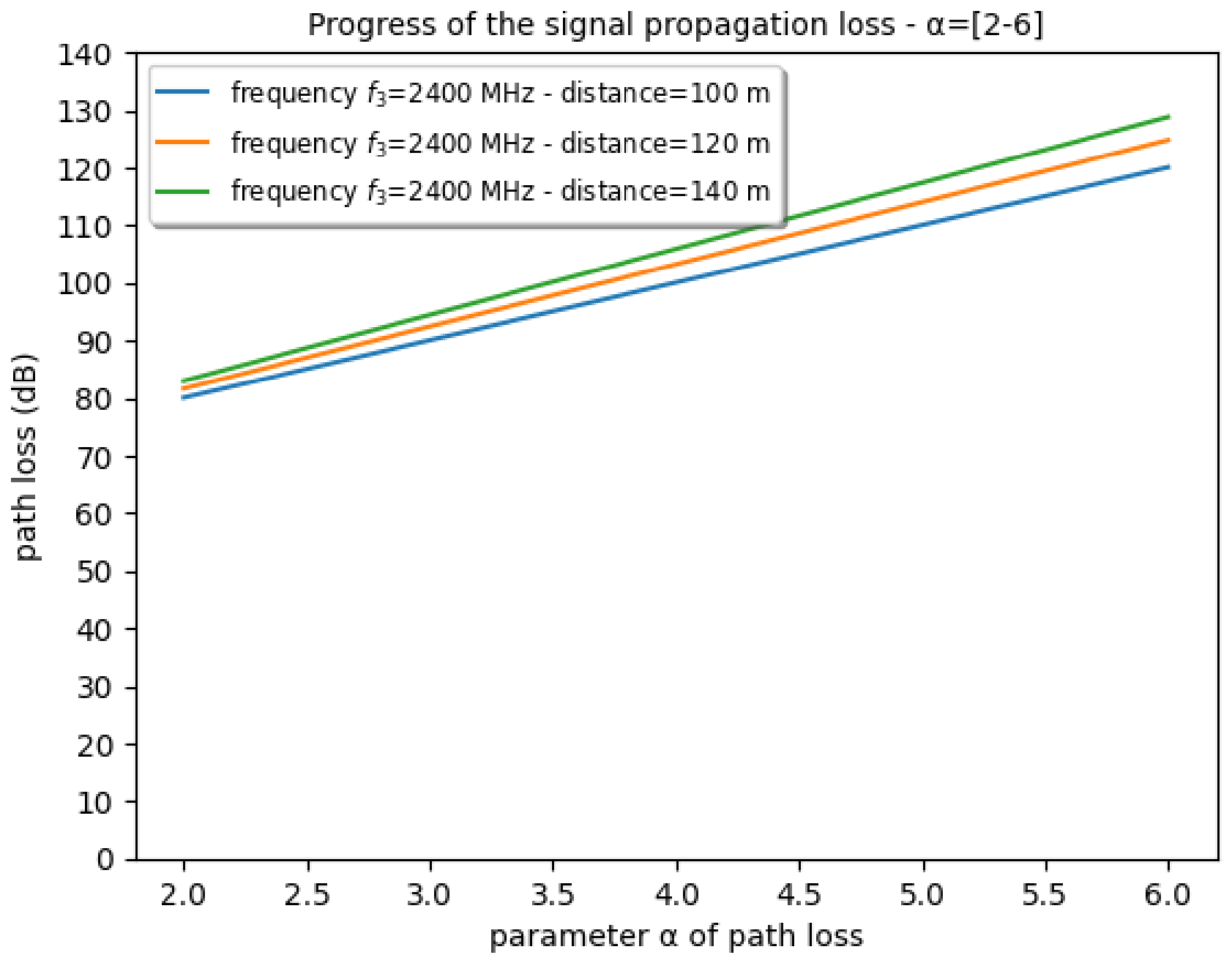
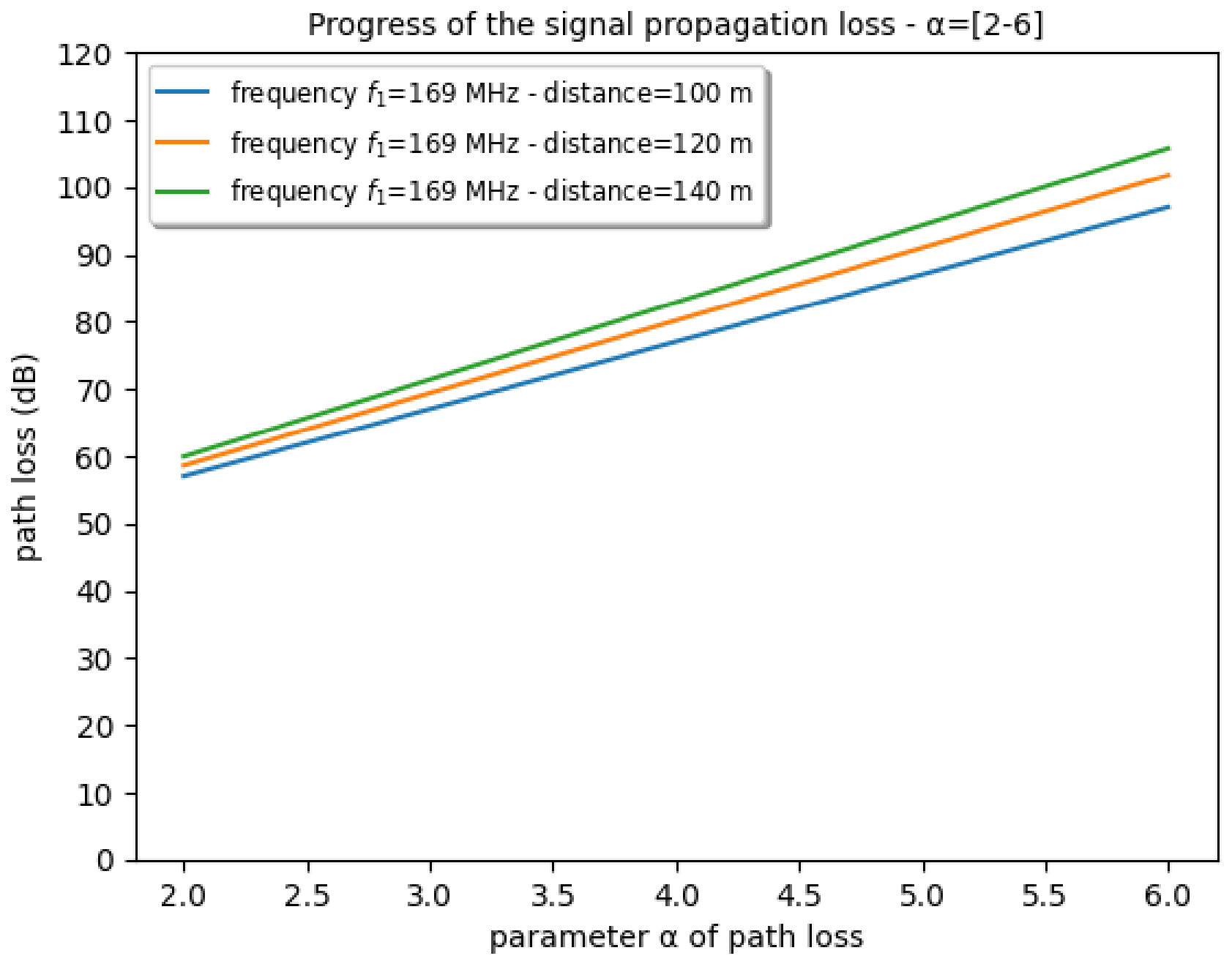
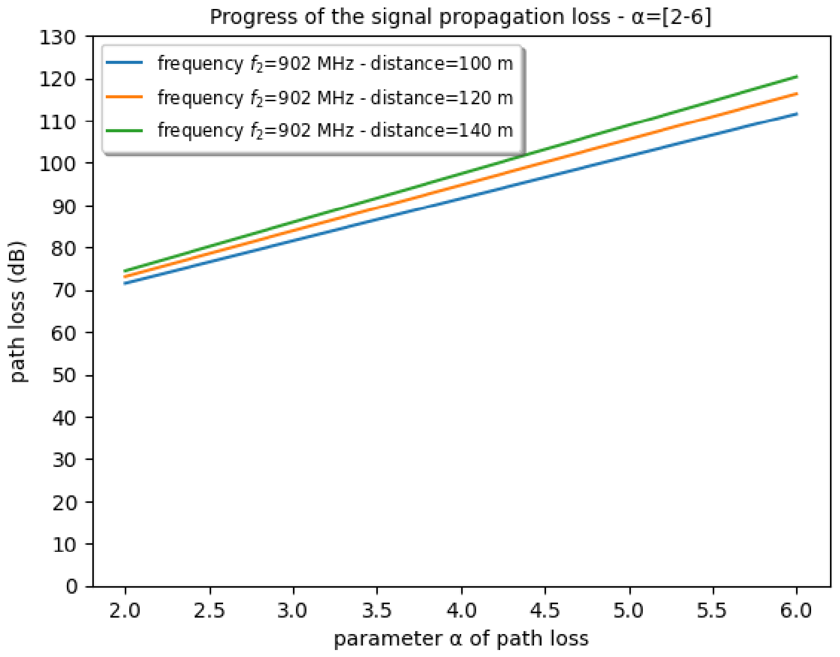
The signal received from data aggregators with two types of smart meters was also evaluated, in which data aggregators can receive information such as voltage and current measurements with a quality signal. Moreover, it was concluded that the premise of a maximum distance $md$ equal to 100 m is true and that it can be extended to 140 m. Signal propagation loss served as an evaluation metric and was integrated into the proposed model in a secondary role in the decision-making process, but ensures low latency in communication between smart meters and data aggregators.

In the literature, some authors claim that reproducibility obtains similar results by using the data and methods described in the papers. Secondly, as stated in ref. [47] and the work of [48], the reproducibility is essential in research to ensure the reliability and validity of scientific results.

To keep the reproducibility of proposed work, in this paper a model was presented as a binary integer nonlinear programming problem and the mathematical linearization technique applied to this model. Beyond that, the terms researched and the databases were described.

The generated instances in several scenarios and the transformation of the optimization problem into a decomposed problem, both according to the literature, were also presented. Other methods were presented to assess the robustness of optimization models in multiple situations. Finally, all technical parameters described below were given their descriptions:

• The cost of data aggregators in a discrete uniform distribution.
• The set of instances with the number of data aggregators and the number of smart meters.
• The area of the planar region.
• The minimum radial distance.
• The maximum budget.
• The Euclidean distances in a metric space.
• The frequencies of operation of the device, such as smart meters and data aggregators.
• All parameters to evaluate the signal propagation loss such as $\alpha$, $d_0$, power of devices, and so on, will be presented.
• Finally, all metrics used in the validation of the methodology will be defined.

In this sense, the reproducibility of the paper can be as ensured as the reliability and validity of the computational results presented.

7. Conclusions

As noted in [7], the smart grid is a novel method of efficiently transmitting power that provides enhanced resilience, flexibility, and reliability in the distribution of electrical power. Beyond that, the use of existing electrical assets is as improved as power management. In addition, the authors highlight that the smart grid is significantly less harmful to the environment than the standard power grid.

Using the concept of smart grid and renewable energy generation, consequently, greenhouse gas emissions can be reduced. Thus, the proposed mathematical model of optimization contributes to smart grids considering the sustainability footprint of electrical power systems.

In addition, this paper presented a new mathematical optimization model to minimize the number of data aggregators in smart grids and assign each smart meter to the data aggregators. A branch–bound algorithm was used to validate this model for several instances. The tests showed optimal performance of an algorithm with low computational time. In addition, the algorithm introduced herein bypasses the need for benchmarking against heuristics or alternative techniques, as it inherently precludes parameter tuning.

The smart meters obtained a ratio ($Rt$) in relation to the allocated data aggregators between 3.8 and 16.7 in the tests presented in this paper. These tests considered a maximum budget and consequently the ratio ($Rt$) was lower than the ratio presented in the literature. The ratio ($Rt$) was reduced due to the fact that the data aggregators were forced to connect more smart meters using the proposed model with budget maximum.

Smart meters are used to improve the quality of electricity and the cost of electricity bills for consumers. The installation of solar panels in their homes for the generation of photovoltaic energy and the adoption of the white tariff are advantageous for the implementation of smart grids. In this sense, smart meters will contribute to a paradigm shift, transforming residential consumers into prosumers.

On the other hand, devices such as data aggregators and smart meters will benefit electricity utilities by generating more profits by reducing non-technical losses and improving the management of the electricity distribution network. In addition, compliance with legal, regulatory and contractual obligations in obedience to ANEEL (National Electric Energy Agency in Brazil) will generate more benefits for the electric power companies. Finally, the model proposed in this work can establish a capital investment limit in the purchase of data aggregators, which will also help the electricity utilities industry.

To validate the proposed framework, simulations were conducted on the IEEE 33-bus radial distribution system, and the results were compared with existing benchmarks.

Moreover, several implications of the findings and practical insights into the results were observed, specifically regarding what these conclusions imply for the design of future architectures in smart grids. These findings have significant implications for the deployment of architectures with the use of data aggregators and smart meters because they prioritize scalability and low latency to accommodate the increasing volume of data from smart meter devices.

The results provide actionable insights for stakeholders involved in smart grid implementation, and offer a blueprint for engineers to optimize data flow within hierarchical grid structures like smart meters and data aggregators. From a practical point of view, the proposed study suggests that the integration of technology with the use of data aggregators is essential to improve the resilience of systems. The results highlight the need for interoperable frameworks that support various communication protocols.

In a wireless communication between a smart meter and a data aggregator, a maximum distance ($md$) is required between these two devices due to path loss. Using two types of smart meters, the signal received was evaluated by data aggregators, indicating that they can receive information with a high-quality signal in several frequencies. Additionally, it was concluded that the assumption of a maximum distance $md$ of 100 m is valid and can be extended to 140 m in the adopted direction.

Thus, for a successful implementation, it is recommended that data aggregators be placed at a maximum distance of 100 to 140 m to minimize packet loss. In addition, the practical insights gained here can guide the development of energy-efficient data processing units for both smart meters and data aggregators.

It was also emphasized that all parameters and strategies were used and presented in this paper to maintain the reproducibility of this work. The reliability and validity of the computational results presented can guarantee the reproducibility of the proposed paper.

The limitations of the paper are as follows: first, it was considered that every consumer has smart meters with wireless communication with good bandwidth; second, the encrypted data for communication between the data aggregators and smart meters was not considered in the proposed model.

Thus, the maximum budget and costs of data aggregators must be different in case the two limitations were considered. For more details on the security of smart grid infrastructures, we suggeste the work of [49] which discusses cybersecurity threats and attacks on smart grids.

Lastly, the optimization mathematical model presented in this paper is a $\mathcal{NP}$-hard problem and can be used in large-scale problems. In this case, metaheuristics can be used to solve large-scale instances with this model. Thus, for future work, we suggest the following metaheuristics: Genetic Algorithm [50] and Iterated Local Search [51]. In addition, the metaheuristics will ensure the following characteristics according to [52], such as exploration (diversification), exploitation (intensification), avoidance of premature convergence, and speed of convergence.