1. Introduction
Heavy metals remain among the most important chemical pollutants in aquatic environments because of their persistence, potential toxicity, and ability to accumulate in environmental compartments and food webs [
1,
2,
3]. In surface waters, metals such as cadmium, lead, and nickel are of particular concern because they may originate from multiple anthropogenic sources, including industrial discharges, mining activities, urban runoff, wastewater effluents, and diffuse catchment inputs [
4,
5,
6,
7,
8]. Their occurrence in rivers and lakes is therefore widely monitored within environmental surveillance frameworks and is frequently considered in water-quality assessment and pollution control [
8,
9,
10,
11].
At the same time, environmental research is increasingly supported by open monitoring databases that provide broad spatial and temporal coverage [
12,
13,
14]. Such datasets offer clear scientific advantages: they enable large-scale comparative analyses, improve reproducibility, facilitate secondary data use, and allow researchers to address questions that would be difficult to investigate within a single local monitoring program [
13,
15,
16,
17]. In water-pollution research, openly accessible monitoring records can therefore serve as an important basis for both descriptive assessments and methodological studies [
13,
14,
18,
19,
20].
However, the analytical value of open monitoring data depends strongly on how these data are prepared before interpretation [
21,
22,
23]. Environmental monitoring records are rarely fully uniform, and their direct use may be affected by differences in water-body categories, analyzed matrices, reporting units, missing values, observation-status codes, and the presence of implausible or otherwise non-comparable observations. In addition, large, harmonized datasets often contain censored measurements reported below the limit of quantification (LOQ), which creates a particularly important methodological problem [
24,
25,
26,
27,
28,
29]. Depending on whether such observations are excluded, replaced by a fraction of the quantification limit, or replaced by the full quantification limit, the resulting concentration summaries and inferred pollution patterns may differ substantially.
Common approaches to handling below-LOQ observations include omission of censored records, simple substitution procedures (e.g., using a fraction of the LOQ or the full LOQ), and more advanced methods for left-censored environmental data, such as regression on order statistics (ROS), Kaplan–Meier-type methods, or likelihood-based approaches [
30,
31,
32]. The choice among these approaches depends on study purpose, data structure, and the degree of censoring [
25,
33,
34]. In large open monitoring datasets, however, simple preprocessing rules remain common because they are transparent, easily reproducible, and directly implementable across heterogeneous records. For this reason, the present study focuses on three scenario-based treatments that reflect routine analytical practice while allowing their downstream effects to be compared explicitly.
This issue is especially relevant for metals monitored at low environmental concentrations, for which censored observations may represent a considerable proportion of the available records [
33,
35,
36,
37,
38]. Under such conditions, preprocessing is not a minor technical step but a factor that can directly influence the interpretation of spatial and temporal patterns. Yet, in many studies using open environmental data, preprocessing choices are reported only briefly, while their effect on the final conclusions is rarely examined systematically. As a result, differences between studies may reflect not only real environmental variation but also different analytical decisions applied before statistical summarization or hotspot identification. This problem is particularly relevant in large-scale water-quality assessments and other harmonized environmental monitoring studies based on secondary open datasets, where preprocessing decisions may substantially shape downstream inference [
22,
39,
40,
41].
A further complication is that open monitoring datasets may contain extreme values that are formally present in the database but are difficult to reconcile with the main empirical distribution and may reflect reporting inconsistencies, harmonization artefacts, or other data-quality problems [
42,
43,
44,
45]. When such values are combined with high proportions of below-LOQ observations, the inferred pollution picture may become highly sensitive to data-handling choices. This is particularly problematic in large-scale assessments intended to compare locations, identify hotspots, or summarize broad regional patterns.
The present study addresses this problem using open European monitoring data for cadmium, lead, and nickel in rivers and lakes. Cadmium, lead, and nickel were selected because they are environmentally relevant heavy metals, widely monitored in open European surface-water datasets [
46,
47,
48,
49]. Rather than treating preprocessing as a purely technical preliminary step, my work considers it a central analytical component of inference from open environmental data. Specifically, the study systematically examines how filtering decisions, treatment of below-LOQ observations, and aggregation choices influence concentration summaries, comparative interpretation across metals, and hotspot identification. In this sense, the systematic aspect of the study lies in the explicit comparison of alternative preprocessing pathways and in tracing how each of them propagates into the final analytical outcomes. The aim of this study was therefore to evaluate how preprocessing decisions influence inferred heavy-metal pollution patterns in open European surface-water monitoring data. Using publicly available records for cadmium, lead, and nickel in rivers and lakes, the study assessed the effects of data filtering, the exclusion of non-comparable observations, the treatment of measurements reported below the limit of quantification, and alternative aggregation strategies on the final statistical summaries and comparative interpretation of pollution patterns.
2. Materials and Methods
2.1. Data Source
The study was based on publicly available water-quality monitoring data obtained from the European Environment Agency (EEA) Waterbase database [
50]. The analysis used disaggregated monitoring records from the Waterbase water-quality dataset, which contains harmonized observations reported by European countries for different water-body categories, determinants, matrices, and sampling dates. The dataset was accessed in SQLite format.
The retained records covered the period 1974–2023. Because the analysis was based on a harmonized multi-country secondary database, the dataset did not reflect one uniform sampling frequency across all records. Instead, monitoring frequency varied across countries, sites, programs, and years, which is an inherent characteristic of large open monitoring compilations of this type [
12,
22,
51,
52].
It should also be noted that the study used secondary data from a harmonized open database and therefore did not rely on a single unified analytical protocol or instrument platform. The original measurements were produced by multiple monitoring authorities and laboratories across different countries and periods, so the underlying analytical methods and equipment may differ between records.
2.2. Selection of Water Categories and Determinants
The study focused on records for three heavy metals: cadmium, lead, and nickel, represented in the database as “Cadmium and its compounds”, “Lead and its compounds”, and “Nickel and its compounds”.
Cadmium, lead, and nickel were chosen due to their environmental relevance, extensive coverage in open European surface-water monitoring datasets, and suitability for a targeted methodological analysis [
46,
47,
48,
49]. In addition, these three determinants showed different proportions of below-LOQ observations, which made it possible to examine how preprocessing sensitivity varies across metals with different censoring structures while maintaining a coherent analytical framework.
The analysis was restricted to inland surface waters, specifically rivers and lakes, corresponding to the Waterbase categories RW (river water bodies) and LW (lake water bodies).
This restriction was introduced to improve comparability and reduce the heterogeneity associated with combining inland waters with coastal, transitional, or territorial waters, which may differ in hydrological characteristics, geochemical background, and monitoring practice. Rivers and lakes also represented the largest and most analytically useful subset of surface-water observations for the selected metals.
2.3. Initial Data Filtering
The first-stage analytical subset was created by retaining only records that met three criteria:
parameterWaterBodyCategory equal to RW or LW;
observedPropertyDeterminandLabel corresponding to cadmium, lead, or nickel;
concentration reported in µg/L.
Inspection of the reported matrices showed that the selected observations were mainly associated with the matrices W, W-DIS, and W-SPM. To avoid mixing whole-water or dissolved-water observations with suspended particulate matter measurements, records from W-SPM were excluded from the main analysis. The final matrix selection therefore retained only W and W-DIS.
Records with missing resultObservedValue were removed. Sampling dates were converted to calendar dates, and the sampling year was extracted for subsequent summarization.
2.4. Sanity Filtering of Implausible Extreme Values
A preliminary exploratory inspection of the filtered dataset revealed a small number of extremely high concentration values that were several orders of magnitude above the main empirical distribution. These observations were concentrated in a limited number of countries and monitoring series and included values that were not plausible for routine heavy-metal concentrations in surface water reported in µg/L. To reduce the influence of likely reporting inconsistencies, harmonization artefacts, or unit-related anomalies, observations with resultObservedValue > 1000 µg/L were excluded from the main dataset.
The threshold of 1000 µg/L was not intended to represent a regulatory, toxicological, or metal-specific environmental boundary. Instead, it was used as a conservative empirical sanity filter to exclude a very small subset of values located several orders of magnitude above the main observed distributions and concentrated in a limited number of countries and monitoring series. Within the scope of this study, the purpose of this step was to reduce the influence of likely reporting anomalies, harmonization artefacts, or unit-related inconsistencies rather than to define a universal concentration limit for environmental interpretation.
This step was intended as a conservative sanity check rather than a substantive environmental threshold. Its purpose was to remove only the most implausible values while preserving the upper tail of the realistic distribution.
2.5. Analytical Datasets
Two related analytical datasets were defined.
The main analytical dataset included all observations that remained after the selection of rivers and lakes, selection of cadmium, lead, and nickel, restriction to µg/L, retention of matrices W and W-DIS, removal of missing concentration values, and exclusion of implausible extreme values above 1000 µg/L. This dataset was used for dataset characterization, descriptive summaries, and evaluation of data retention across preprocessing steps.
The censoring-analysis dataset was derived from the main analytical dataset and used specifically to compare alternative treatments of below-LOQ observations. In this dataset, all observations not reported below the limit of quantification were retained, whereas observations flagged as below LOQ were retained only if a corresponding procedureLOQValue was available. Below-LOQ records without an available LOQ value were excluded from the censoring-scenario comparison.
2.6. Treatment of Below-LOQ Observations
Because a substantial proportion of observations for the selected metals were reported below the limit of quantification, three alternative censoring scenarios were compared:
Scenario A: removal of below-LOQ observations—all records flagged as below LOQ were excluded;
Scenario B: substitution with half the LOQ—for records flagged as below LOQ, the final concentration value was set to 0.5 × procedureLOQValue;
Scenario C: substitution with the full LOQ—for records flagged as below LOQ, the final concentration value was set to 1.0 × procedureLOQValue.
These scenarios were chosen to represent three common and transparent approaches to handling censored environmental observations. Their comparison allowed the sensitivity of inferred pollution patterns to be evaluated directly.
The scenarios were selected not as an exhaustive representation of all available statistical methods for censored environmental data but as simple and commonly encountered preprocessing strategies that remain relevant in routine data handling. This design was consistent with the aim of the study, namely, to evaluate how transparent and easily reproducible preprocessing choices influence downstream inference in open monitoring datasets.
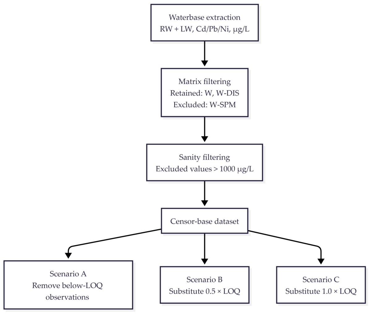
The overall preprocessing workflow applied in this study is summarized in
Figure 1. Starting from the Waterbase extraction for cadmium, lead, and nickel in rivers and lakes, the workflow included matrix-based harmonization, exclusion of implausible extreme values, construction of a censor-base dataset, and implementation of three alternative censoring scenarios for below-LOQ observations. This workflow was designed to treat preprocessing not as an implicit technical background step but as an explicit component of the analytical framework.
2.7. Descriptive and Comparative Analysis
The analysis focused on how preprocessing choices influenced the statistical description of concentration patterns for cadmium, lead, and nickel. For each scenario and each metal, the following descriptive measures were calculated: number of observations, median, mean, 90th percentile, 95th percentile, 99th percentile, and maximum value.
These summaries were used to compare how censoring treatment affected central tendency and upper-tail behavior. Additional descriptive comparisons were performed for rivers and lakes separately to evaluate whether the broad interpretation of results remained consistent across the two inland surface-water categories.
2.8. Sensitivity Framework
The study was designed as a methodological sensitivity analysis rather than a regulatory assessment of compliance status. Accordingly, the main objective was not to estimate definitive pollution levels for Europe but to examine the extent to which inferred patterns depend on preprocessing decisions. Sensitivity was assessed by comparing how alternative analytical choices changed the number of observations retained, the proportion of censored records, the resulting concentration summaries, and the comparative interpretation across metals and water-body categories.
This framework allowed preprocessing to be treated as an explicit object of analysis rather than an unreported technical background step.
2.9. Software
Data extraction, preprocessing, and statistical summarization were performed in Python 3.13.9 (Anaconda distribution) using standard data-processing tools for SQLite based workflows (SQLite version 3.51.0, via the Python sqlite3 module) and tabular analysis implemented in Spyder 6.1.0.
3. Results
3.1. Data Retention After Successive Filtering Steps
The effect of successive preprocessing steps on dataset size is summarized in
Table 1. The largest reductions in record number were associated with matrix harmonization and the construction of the censor-base dataset, whereas the exclusion of implausible extreme values affected only a small fraction of observations.
The initial analytical extraction from the Waterbase database included cadmium, lead, and nickel records from rivers and lakes, reported in µg/L. After restricting the dataset to the matrices W and W-DIS and removing observations with missing concentration values, the resulting dataset contained 1,478,614 observations. Further exclusion of implausible extreme values above 1000 µg/L yielded a main analytical dataset of 1,475,409 observations.
Within this dataset, nickel accounted for 520,366 observations, lead for 504,449, and cadmium for 450,594. Rivers clearly dominated the dataset, accounting for 1,484,161 observations in the pre-cleaned subset, whereas lakes contributed 185,296 observations. The filtered dataset covered a long temporal range, from 1974 to 2023, although most records were concentrated in more recent years. The median sampling year was 2015, with the interquartile range spanning approximately 2009 to 2018, indicating that the final dataset mainly reflects contemporary monitoring practice.
3.2. Prevalence of Below-LOQ Observations
The prevalence of below-LOQ observations and the completeness of LOQ metadata for the analyzed metals are presented in
Table 2.
A substantial proportion of the cleaned observations was reported below the limit of quantification. In the main analytical dataset, below-LOQ records accounted for 66.6% of cadmium, 57.3% of lead, and 36.1% of nickel observations. This confirms that censored observations were not a marginal feature of the selected data but a central structural characteristic of the dataset.
Because the comparison of censoring scenarios required an explicit LOQ value, a dedicated censoring-analysis dataset was created by retaining all non-censored observations and only those below-LOQ observations for which procedureLOQValue was available. This reduced the dataset to 1,259,636 observations. The excluded subset consisted entirely of below-LOQ observations without available LOQ values and amounted to 91,197 records for cadmium, 74,811 for lead, and 49,765 for nickel. Overall, 27.76% of below-LOQ observations in the cleaned dataset lacked an explicit LOQ value and could not be used in the scenario-based substitution analysis.
Even after this additional restriction, censored observations remained highly prevalent. In the censoring-analysis dataset, below-LOQ records represented 58.1% of cadmium observations, 49.8% of lead observations, and 29.4% of nickel observations, indicating that the influence of censoring treatment was expected to differ across metals.
3.3. Effect of Censoring Treatment on Concentration Summaries
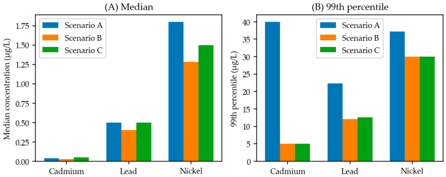
Observation-level concentration summaries under the three censoring-treatment scenarios are given in
Table 3 and visualized in
Figure 2.
The choice of censoring strategy clearly affected the inferred concentration distributions for all three metals, although the magnitude of this effect differed substantially between them. The strongest response was observed for cadmium. Under Scenario A, in which below-LOQ observations were removed, the median concentration was 0.040 µg/L, compared with 0.028 µg/L under Scenario B and 0.050 µg/L under Scenario C. The effect on upper-tail summaries was even more pronounced: the 99th percentile reached 40.0 µg/L under Scenario A, compared with 5.0 µg/L under both substitution scenarios.
Lead showed the same general pattern, although less strongly than cadmium. The median concentration was 0.500 µg/L under Scenario A, 0.400 µg/L under Scenario B, and 0.500 µg/L under Scenario C. The 99th percentile was 22.3 µg/L under Scenario A, compared with 12.1 µg/L and 12.6 µg/L under Scenarios B and C, respectively.
For nickel, censoring treatment still affected the results, but the magnitude of change was smaller. The median concentration was 1.800 µg/L under Scenario A, 1.280 µg/L under Scenario B, and 1.500 µg/L under Scenario C. The 99th percentile was 37.2 µg/L under Scenario A and 30.0 µg/L under both substitution scenarios.
Taken together, these results show that omission of below-LOQ observations systematically increased concentration summaries and that the magnitude of this effect was related to the proportion of censored records. Among the three metals analyzed, cadmium showed the strongest sensitivity to censoring treatment, followed by lead, whereas nickel was comparatively more stable.
The rank order of scenario sensitivity closely followed the censoring structure reported in
Table 2. Cadmium, which had the highest proportion of below-LOQ observations, showed the strongest upward shift under Scenario A, whereas nickel, with the lowest censoring percentage, showed the smallest scenario dependence. This pattern provides a mechanistic explanation for why removal of below-LOQ observations leads to the strongest distortion in metals with the greatest degree of censoring.
3.4. Comparison Between Rivers and Lakes
When the half-LOQ substitution scenario was used as a reference framework, the general patterns observed for rivers and lakes were broadly similar, although some quantitative differences were evident. For cadmium, the median concentration was 0.030 µg/L in rivers and 0.025 µg/L in lakes, while the 99th percentile was 5.0 µg/L in rivers and 3.0 µg/L in lakes. For lead, the median was 0.400 µg/L in rivers and 0.300 µg/L in lakes, whereas the 99th percentile reached 13.6 µg/L in rivers and 5.0 µg/L in lakes. For nickel, the medians were very similar in rivers and lakes (1.29 µg/L and 1.25 µg/L, respectively), whereas upper percentiles differed somewhat more, with the 99th percentile equal to 30.0 µg/L in rivers and 28.188 µg/L in lakes.
These results suggest that the broad comparative interpretation of the three metals was not fundamentally different between rivers and lakes, which supports the use of a combined inland surface-water analytical framework. At the same time, the somewhat higher upper-tail values observed in rivers, especially for cadmium and lead, indicate that water-body category may still influence the magnitude of inferred pollution patterns and should therefore be considered in supplementary comparisons.
3.5. Station-Year Concentration Summaries Under Alternative Censoring-Treatment Scenarios
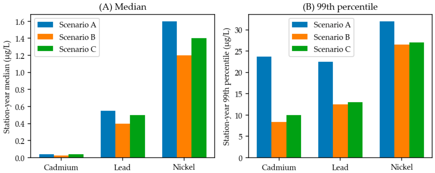
Table 4 and
Figure 3 show that the effect of censoring treatment remained evident after aggregation to the station-year level, indicating that preprocessing sensitivity was not limited to raw observation distributions.
The influence of censoring treatment remained evident after aggregation to the station-year level. Across all three metals, the removal of below-LOQ observations produced higher station-year medians and upper percentiles than substitution-based approaches. The strongest effect was again observed for cadmium, for which the station-year median increased from 0.025 µg/L under the half-LOQ scenario to 0.040 µg/L under the omission scenario, while the 99th percentile increased from 8.38 to 23.68 µg/L. Lead showed an intermediate response, whereas nickel remained comparatively more stable.
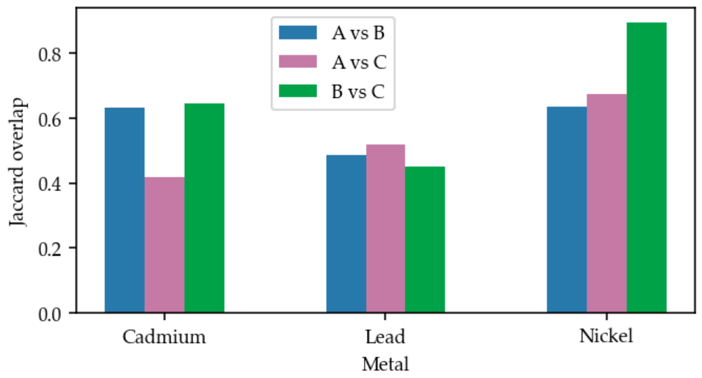
The effect of preprocessing was also visible in hotspot identification. When station-year units above the 95th percentile of station-year medians were treated as hotspots, the overlap between scenarios varied substantially across metals. For nickel, hotspot composition was highly stable between the half-LOQ and full-LOQ substitution scenarios (Jaccard overlap = 0.897). In contrast, cadmium and lead showed markedly lower overlap values, particularly when omission of below-LOQ observations was compared with substitution-based scenarios. These results indicate that preprocessing choices can affect not only concentration summaries but also the identification of locations and periods interpreted as the most polluted.
The overlap between station-year hotspot sets identified under the alternative censoring scenarios is summarized in
Table 5 and visualized in
Figure 4.
3.6. Summary of the Main Sensitivity Pattern
Across all analyses, the dominant source of variability in inferred concentration patterns was the treatment of observations reported below the limit of quantification. Other preprocessing steps, such as restriction to comparable water categories, exclusion of suspended-particulate measurements, removal of missing values, and filtering of implausible extremes, were necessary to establish a coherent analytical dataset. However, once this dataset was defined, censoring treatment became the main factor shaping the final statistical picture.
The sensitivity ranking was consistent across summary measures and closely followed censoring prevalence: cadmium showed the strongest response, lead an intermediate response, and nickel the lowest. This indicates that the proportion of below-LOQ observations is a key determinant of methodological stability in open monitoring-based pollution assessments.
4. Discussion
4.1. Influence of Censoring Treatment on Inferred Pollution Patterns
The study showed that preprocessing choices substantially influence the interpretation of open inland surface-water monitoring data for heavy metals. Although the analyzed Waterbase records provided broad spatial and temporal coverage and a very large number of observations, the final statistical picture proved highly sensitive to how the dataset was filtered and, above all, how censored observations were handled. This confirms that open environmental data are not analytically neutral and that their large scale does not eliminate the need for careful methodological control.
A central finding of this study is that observations reported below the limit of quantification were not a minor technical detail but a dominant structural feature of the dataset. Even after harmonization and cleaning, below-LOQ records accounted for 66.6% of cadmium observations, 57.3% of lead observations, and 36.1% of nickel observations in the main analytical dataset. As a result, concentration summaries derived from such data depend, at least in part, on the censoring strategy applied. The results clearly showed that omission of below-LOQ observations systematically shifted concentration summaries upward, especially for cadmium and, to a lesser extent, for lead. In practical terms, analyses based only on detected values may overstate both central tendency and upper-tail distribution properties when censoring is widespread.
Beyond the simple LOQ substitution rules compared here, more advanced approaches for left-censored environmental data, such as regression on order statistics (ROS), Kaplan–Meier-type methods, or likelihood-based techniques, could provide a useful additional benchmark [
30,
33,
34]. However, the present study was designed primarily to evaluate how simple, transparent, and still commonly used preprocessing choices affect downstream inference in open monitoring datasets. For this reason, the analysis deliberately focused on three scenario-based treatments that are easy to interpret, reproducible, and directly relevant to routine analytical practice. A more formal benchmark against censored-data modeling approaches remains an important direction for future work.
The strongest sensitivity was observed for cadmium, which is consistent with its highest proportion of censored observations. Lead showed an intermediate response, whereas nickel was comparatively more stable. This pattern suggests that methodological sensitivity is closely related to censoring prevalence: the more frequently a determinant is reported below LOQ, the more strongly the final interpretation depends on the handling rule applied.
This also points to a broader analytical gap in environmental monitoring. The substances of greatest toxicological concern are often those monitored at very low environmental concentrations and therefore those most strongly affected by censoring [
33,
53,
54]. In practical terms, the metals of greatest interpretive concern may simultaneously be those for which analytical limitations and preprocessing choices exert the strongest influence on the final statistical picture.
The comparison between censoring scenarios also has a practical implication for the interpretation of pollution summaries. The removal of censored observations produced the highest medians and upper percentiles for all three metals, whereas substitution-based approaches yielded lower and generally more stable summaries. Such behavior indicates that the removal of below-LOQ observations does not simply reduce sample size, it also alters the shape of the retained distribution by selectively discarding low-end observations. Consequently, analyses that do not explicitly report how censored data were treated may be difficult to compare, even when they rely on the same underlying monitoring source.
4.2. Sensitivity After Station-Year Aggregation and Hotspot Identification
Importantly, the dependence on censoring treatment did not disappear after aggregation to the station-year level. This matters because station-year summaries represent a more integrated analytical unit that is closer to practical monitoring interpretation than individual measurements. Even after aggregation, omission of below-LOQ observations produced higher medians and upper percentiles than substitution-based scenarios, and the same sensitivity ranking (cadmium > lead > nickel) remained evident.
Preprocessing choices also affected hotspot identification. When station-year units at or above the 95th percentile of station-year medians were treated as hotspots, the overlap between hotspot sets varied substantially across censoring scenarios (
Table 5,
Figure 4). Hotspot composition was highly stable for nickel between the two substitution approaches, whereas cadmium and lead showed markedly lower overlap when omission-based and substitution-based workflows were compared. This demonstrates that preprocessing can influence not only the magnitude of inferred concentrations but also the identity of the locations and periods interpreted as most pollution-prone, i.e., an outcome with practical relevance for screening, prioritization, and comparative interpretation.
4.3. Harmonization and Data-Quality Issues in Open Monitoring Datasets
The analysis also illustrates that meaningful use of large open monitoring databases requires explicit harmonization beyond censoring alone. The initial extraction contained multiple water-body categories, different analyzed matrices, missing values, and a small subset of implausibly high observations. Restriction to inland surface waters (rivers and lakes), exclusion of non-comparable matrices (notably W-SPM), and removal of missing concentration values were necessary to establish an analytically coherent dataset. The additional sanity filtering of extreme values served to prevent clearly unrealistic observations—potentially reflecting reporting inconsistencies, harmonization artefacts, or unit anomalies—from dominating summary statistics.
These steps highlight a general point: open monitoring data provide scale and coverage, but they also embed heterogeneity in sampling design, reporting conventions, and metadata completeness. Treating preprocessing as an explicit part of the analytical framework is therefore essential for interpretability and reproducibility, particularly when datasets are reused by different researchers under different conventions.
The comparison between rivers and lakes suggests that combining the two inland categories is acceptable for a methodological sensitivity analysis of this type. Under the reference substitution scenario, rivers tended to show somewhat higher upper-tail values than lakes for some metals, but the relative behavior across censoring scenarios remained broadly consistent. For the present purpose, i.e., quantifying sensitivity to preprocessing rather than producing category-specific typologies, this combined inland framework is therefore justified.
4.4. Limitations
An important limitation of the censoring analysis is that not all below-LOQ observations could be retained. More than one quarter of censored records lacked an explicit LOQ value and therefore could not be incorporated into substitution-based scenarios. This appears to reflect metadata incompleteness in the harmonized source database rather than an analytical decision introduced in the present study. In other words, some observations were flagged as being below LOQ, but the corresponding procedureLOQValue field was not populated in the available record. This limitation is itself informative, because it shows that even when a dataset explicitly indicates censoring, the information required for transparent downstream handling may still be incomplete.
My study should also be interpreted considering its intended scope. The goal was not to produce a definitive regulatory assessment of heavy-metal pollution in Europe, nor to identify policy-relevant exceedances for specific sites. Instead, the analysis was designed to evaluate the sensitivity of inferred concentration patterns to preprocessing decisions. For that reason, the study focused on transparent descriptive summaries, scenario comparison, and hotspot stability rather than on regulatory thresholds, ecological classification schemes, or formal exposure assessment. This delimitation is important because it clarifies that the main contribution lies in methodological inference. The results therefore do not replace formal status assessments, but they do show that the preprocessing pipeline can meaningfully alter the evidence base on which broader interpretations might be built.
A further limitation is that the analysis was intentionally restricted to three metals and two inland surface-water categories. This was done to improve comparability and maintain a focused methodological design, but it also means that the results should not automatically be generalized to all pollutant classes or all water-body types represented in the source database. Similarly, although the study included broad European coverage, it did not attempt a country-specific decomposition of the observed patterns. Part of the sensitivity documented here may therefore reflect differences in national monitoring practice, reporting conventions, or metadata completeness, rather than only differences intrinsic to the behavior of the analyzed metals.
4.5. Implications and Future Research
From a broader perspective, the shown findings support a more explicit culture of reporting in open-data environmental research. When large monitoring datasets are reused, it is often assumed that scale and official provenance are sufficient to ensure interpretive robustness. The present results suggest otherwise. Open monitoring data can indeed provide strong analytical value, but only when the workflow used to prepare them is described in enough detail to allow readers to judge how the conclusions were produced. At minimum, such reporting should include the selected water categories, matrices, units, treatment of missing values, criteria for excluding implausible observations, and explicit handling of below-LOQ records. Without such transparency, apparent differences between studies may reflect workflow choices as much as environmental reality.
My study also opens several directions for future work. First, the effect of preprocessing could be tested on additional metals or other groups of pollutants with high censoring prevalence. Second, aggregation choices could be explored further at other analytical levels, such as station, station-year, or regional summaries, to determine whether hotspot identification is more sensitive than global descriptive statistics across different spatial scales. Third, country-level or region-specific subsets could be analyzed separately to investigate whether part of the observed methodological instability reflects differences in pollution level, national monitoring practice, reporting conventions, or metadata completeness rather than only pollutant behavior. Such extensions would help distinguish between intrinsic statistical sensitivity and dataset-structure sensitivity.
The general framework used in this study is not limited to cadmium, lead, and nickel and may also be applied to other heavy metals or, more broadly, to other monitored chemical determinants. However, the relative importance of preprocessing steps is likely to depend on the environmental concentration regime of the analyzed substance. For elements that typically occur at very low concentrations, such as mercury or arsenic [
55,
56,
57], high proportions of below-LOQ observations may make the results even more sensitive to censoring treatment. In contrast, for elements that may occur at much higher concentrations, such as iron in groundwater or mining-influenced waters [
58,
59], censoring may play a smaller role, while other preprocessing decisions, including plausibility filtering and matrix comparability, may become more important.
For applied researchers using large open monitoring datasets, the main practical implication is that datasets with high proportions of below-LOQ observations should not be interpreted solely after removing nondetects, because this approach can systematically inflate concentration summaries and alter hotspot identification. At minimum, studies should report the censoring percentage, explicitly state the handling rule used for below-LOQ observations and, where feasible, compare more than one preprocessing scenario. Such reporting would improve both interpretability and comparability across studies using harmonized open environmental data.
Overall, the main message is clear: preprocessing is not a peripheral technical step in the analysis of open monitoring data but a central determinant of the conclusions that can be drawn from them. In the present dataset, handling censored observations was the dominant driver of variation in concentration summaries, and this effect was strongest for the metal with the highest proportion of below-LOQ values. The effect persisted after station-year aggregation and influenced hotspot identification. Therefore, any comparative interpretation of open heavy-metal monitoring data should be accompanied by explicit and reproducible reporting of preprocessing choices, particularly those involving LOQ-related decisions.
5. Conclusions
The study performed showed that the interpretation of open inland surface-water monitoring data for heavy metals is strongly influenced by preprocessing decisions. Using publicly available European records for cadmium, lead, and nickel in rivers and lakes, it was demonstrated that data filtering, the exclusion of non-comparable observations, sanity control of implausible extremes, and especially the treatment of below-LOQ measurements can substantially alter concentration summaries and inferred pollution patterns.
The final analytical dataset remained very large after harmonization and cleaning, confirming the substantial value of open monitoring resources for large-scale environmental analysis. At the same time, the results showed that the dataset structure itself creates important methodological challenges. A high proportion of observations was reported below the limit of quantification, reaching 66.6% for cadmium, 57.3% for lead, and 36.1% for nickel. In addition, more than one quarter of below-LOQ records lacked an explicit LOQ value and therefore could not be used in substitution-based scenarios.
Among the examined preprocessing choices, censoring treatment was the dominant source of analytical sensitivity. Removal of below-LOQ observations systematically increased medians and upper percentiles relative to substitution-based approaches, with the strongest effect observed for cadmium, an intermediate effect for lead, and the lowest effect for nickel. This ranking remained consistent after aggregation to the station-year level, indicating that the sensitivity was not limited to raw measurements but also affected more integrated summaries relevant to practical monitoring interpretation.
The analysis further showed that preprocessing choices influence not only descriptive statistics but also hotspot identification. The composition of station-year hotspot sets varied across censoring scenarios, particularly for cadmium and lead, demonstrating that alternative handling of censored observations may change which locations and periods are interpreted as the most pollution-prone. This finding reinforces the conclusion that preprocessing is not a purely technical background step but a central component of inference from open monitoring data.
Overall, the study supports three main conclusions. First, open environmental monitoring databases provide a powerful basis for pollution research, but they require explicit harmonization and quality control before interpretation. Second, the handling of censored observations must be treated as a methodological decision with direct consequences for the final results. Third, transparent and reproducible reporting of preprocessing workflows is essential if studies based on open monitoring data are to remain interpretable and comparable.
Although the present analysis was restricted to rivers and lakes, the general methodological framework may also be transferred to other monitored water environments, including groundwater and spring systems. In such cases, the workflow would need to be adapted to the specific hydrochemical background, concentration ranges, monitoring design, and matrix comparability of the studied system. Therefore, the approach should be understood as transferable but not universally identical in its practical implementation.
In particular, datasets with high proportions of below-LOQ observations should not be interpreted solely after removing nondetects, because this approach may systematically inflate concentration summaries and alter hotspot identification. For applied use, a practical hierarchy of preprocessing should begin with the explicit reporting of censoring prevalence, followed by clear documentation of the rule used for handling below-LOQ records and, where feasible, comparison of more than one preprocessing scenario.
In practical terms, future studies using large open water-quality datasets should report, at minimum, the selected water categories, analyzed matrices, units, missing-data treatment, criteria for excluding implausible observations, and exact rule used for handling below-LOQ records. Without such transparency, differences between studies may reflect workflow choices as much as real environmental variation.