Ultrasonic Frequency Analysis of Adhesively Bonded Joints ^†

Abstract

Bonded joints are commonly used for aircraft construction. The non-destructive testing of these components for debonds can be performed using traditional NDI. However, in the case of weak bonds and “kissing bonds”, inspection becomes more difficult. In this work, we have investigated weak bonds that have been produced by contaminating the bondline interface with different release agents. By carrying out an analysis of ultrasonic data from the frequency domain, the bondline thickness can be determined. Additionally, indications of the presence of contaminants/weak bonds can be detected at specific frequencies, while the effects of a non-uniform bondline thickness can be suppressed by averaging the power around the selected frequency. Mechanical testing at different locations showed that indications in the frequency domain were able to find one weak bond, while the other indications showed no decrease in lap shear strength.

1. Introduction

The use of adhesively bonded metals in aircraft structures has become increasingly popular in recent years, particularly in the construction of fuselages and empennages. This joining technique offers several advantages over traditional mechanical fastening methods, including a reduced weight, increased structural integrity, and improved fatigue resistance. In aircraft fuselages, adhesively bonded metals are used to join stringers, frames, and skin panels, creating a strong and lightweight structure. The adhesive bonding process allows for the creation of complex geometries and the joining of dissimilar materials, enabling the design of optimized structural components.

To ensure the integrity of adhesively bonded joints in aircraft structures, various NDI techniques are employed, such as ultrasonic testing, X-ray Radiography, and Resonance testing (e.g., the Fokker Bond tester). Depending on the defect type, one or another technique may more suitable. The main challenge for NDI techniques lies in detecting weak or “kissing bonds”, where the bonds have less strength than normal but are overlooked when using traditional NDI techniques. Traditionally, the Fokker Bond tester has been used to detect debonds between adhesively bonded metal sheets, as by using Fokker Bond tester correlation graphs the approximate cohesive strength of the bond can be determined [1]. However, the Fokker Bond tester is an old, time-consuming, and manual technique, so alternatives are being sought. Using ultrasonic pulse-echo data and machine learning has been shown to be a potential technique for detecting weak and/or kissing bonds [2]. Additionally, the combination of different techniques also shows potential [3].

In this work, ultrasonic through-transmission (TT) has been carried out on adhesively metal bonded sheets. This analysis is performed in the frequency domain, providing more information that is potentially useful for detecting weak and/or “kissing bonds”.

2. Materials and Methods

Reference specimens were supplied by GKN Aerospace, Papendrecht, The Netherlands. Two types of reference specimens will be discussed. Both types of reference specimens are made of two 400 × 400 × 1.6 mm³ aluminum sheets (AA 2024–T3 AL clad) that are bonded together using the 3M^tm Scotch-Weld^tm structural adhesive film AF163-2K.06WT, which has a nominal thickness of 0.15 mm. The first type of reference specimen contains inserts of flash breaker tape and the backing paper of the adhesive film; these samples are called insert panels. Figure 1a shows the size and location of the inserts. The flash breaker tape was put on top of the adhesive, while adhesive was cut up in order to incorporate the backing paper into the structure. This panel was cured in an autoclave using a standard procedure. As for the second type of panel, contaminants were added onto the adhesive in order to reduce its strength; these panels are called “Kissing bond” (KB) panels. The first type of contaminant was a release agent, Marbocoat 227. The second type was silicon oil. Figure 1b shows the pattern of how these contaminants were applied to the panel. Due to the presence of silicon oil, the panel was not cured in the production autoclave, instead a heated press was used.

Two types of methods have been employed to investigate the panels: ultrasonic through-transmission (TT) and 3D structured-light scanning. Ultrasonic TT was performed using the USL C-scan system. Squirters with a nozzle diameter of 6 mm were used. Scanning was performed at an index of 1 mm with a sample frequency of 250 MSPS. Broad-band transducers with nominal frequencies of 1, 5, and 10 MHz have been used. Three-dimensional structured-light scanning was carried out using the Zeiss ATOS5, with a measuring volume of MV 320 × 240 × 240 mm³, in order to measure the thickness of the samples. Data processing was performed in Matlab. Single lap shear tensile testing was performed using an Instron 68FM-100 tensile machine. The lap shear samples had a width of 25 mm and a total length of 187.5 mm. The overlap area had a length of 12.5 mm, resulting in an overlap area of 25 × 12.5 mm². The testing speed was set to 1.00 mm/min.

3. Results

3.1. Standard Through-Transmission

Figure 2 shows the results of the TT signal for the Insert and KB panels, respectively. The maximum amplitude of the rectified A-scans are plotted as a C-scan. In this though-transmission (TT) scan, all the inserts included in the insert panel can be detected, with an attenuation of about −13 dB. In the pristine area of the insert panel, clear banding can be seen, indicating areas of low and high attenuation. In the KB panel, a large debond is detected where the large circular spot of Marbocoat 227 was applied; the other areas that were contaminated show little-to-no attenuation.

3.2. Three-Dimensional Structured-Light Scanning

Three-dimensional structured-light scanning was performed to assess the total thickness of the samples. Figure 3 shows the results for the insert and KB panels. The insert panel shows a lot of deviation in its total thickness. Its minimum thickness measured is as 3.31 mm and its maximum thickness amounts to 3.51 mm in the center of the panel. Before gluing, the single sheets were also measured and were within tolerance (±0.05 mm) and quite straight. Therefore, the thickness variation in the insert panel can only be attributed to a change in bondline (BL) thickness. In the insert panel, the BL thickness ranges from 0.09 at the edges to 0.31 mm at the center. The KB panel, which was made in a press, shows a much more uniform thickness compared to the insert panel. For this panel, the BL thickness ranges from 0.10 to 0.22 mm.

The banding in Figure 2 occurs due to the difference in the thickness of the BL, and will be explained in more detail in Section 3.3.

3.3. Frequency Analysis

All the ultrasonic volume data for the panel were captured, such that the A-scan data for each pixel are available. This enables a frequency analysis of the A-scan signal at each pixel shown within the C-scan. The A-scan was recorded over 7500 samples (30 µs). A Fourier transformation was applied in Matlab, giving the amplitude at each frequency interval (Δf = 33.3 kHz). First, for each of the transducer pairs (1, 5, and 10 MHz) the A-scan signal was recorded without a panel in between the transducer pair, resulting in the total response of the system, as shown in Figure 4a for 10 MHz. Subsequently, the sample was put in between the transducers and the overall gain of the system was modified such that the maximal signal reached about 80% of the full screen height. Figure 4b shows the results for the two 10 MHz transducers, and the spectrum of the sample was taken from a pristine spot. The signal has a center frequency of 7.78 MHz and a −6 dB bandwidth of 4.12 MHz, without the aluminum reference sample in between.

The aluminum bonded sample that was put between the transducers acts as a frequency filter, suppressing a lot of frequencies that are present in the water-to-water path. In this case, the frequencies inside of a single sheet of material are dominated by multiples of ½ a wavelength (~2, 4, 6, 10, 12, 14 MHz). Resonance frequencies from the bondline are also visible in the graph (marked by the red circles), and these frequencies are mainly determined by the thickness of the BL. By identifying these resonance peaks, the thickness of the BL can be calculated. Figure 5a shows the frequency of the resonance peak between 4.5 and 5.6 MHz from the insert panel. The center of the panel shows a resonance peak that is close to 4.5 MHz and this frequency increases farther away from the center. Using the frequency of this resonance peak, the thickness of the BL can be calculated by assuming a constant speed in the epoxy, which is taken to be 2800 m/s. The maximum BL thickness is calculated (d_BL = ½ × v_epoxy/f_res) to be 0.31 mm in the center of the panel and decreases closer to the edges; see Figure 5b. The obtained pattern closely resembles the 3D scan shown in Figure 3. If the assumption is made that the metal sheets have a combined thickness of 3.2 mm, the maximum thickness from the UT data corresponds to 3.5088 mm, which is in agreement with the 3D scan in terms of both the values and the overall picture. In this case, only the frequency range between 4.5 and 5.6 MHz was selected, such that the resonance peaks of the 1.6 mm sheets were skipped. When the resonance frequency of the BL corresponds to the sheet thickness it difficult to distinguish the resonance peaks of the BL. The BL thickness in the areas close to the edges of the sheet is lower, resulting in higher resonance frequencies which are not taken into account with this method. This section shows that by tracking the resonance frequencies, the BL thickness in a single-bondline sheet can be determined using a frequency analysis of its ultrasonic TT signal. This same phenomena produces the banding that is visible in the “standard” UT TT images.

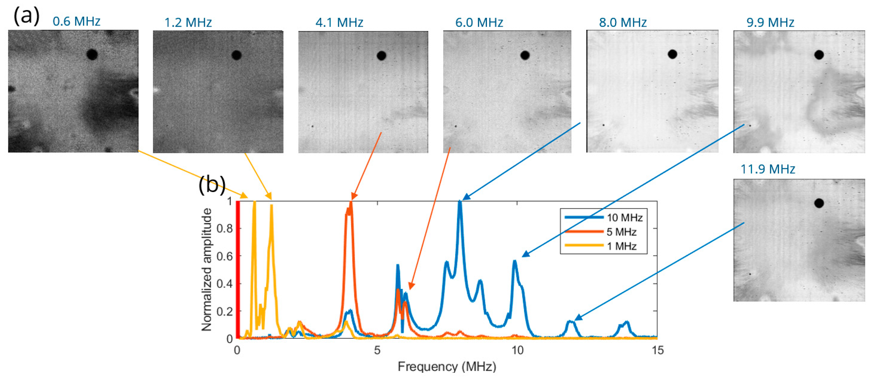
Figure 6 shows the amplitude images at specific frequencies (normalized at each frequency step for better visibility) for the KB panel. All transducers were used and the frequency spectrum in the center of the panel is plotted in the figure as well. With the 1 MHz transducer, two peaks can be seen. The image at 8.0 MHz more or less corresponds to the TT image shown in Figure 2, since the TT image uses the maximum in the time domain and the 8 MHz plot uses the global maximum in the frequency domain. When looking at the other pictures, the results look similar. All images show a debond in the right upper corner of the panel, and at high frequencies the larger total thickness on the right side of the sample can also be seen.

However, the amplitude images at the shoulders of the main peaks show a lot more information.

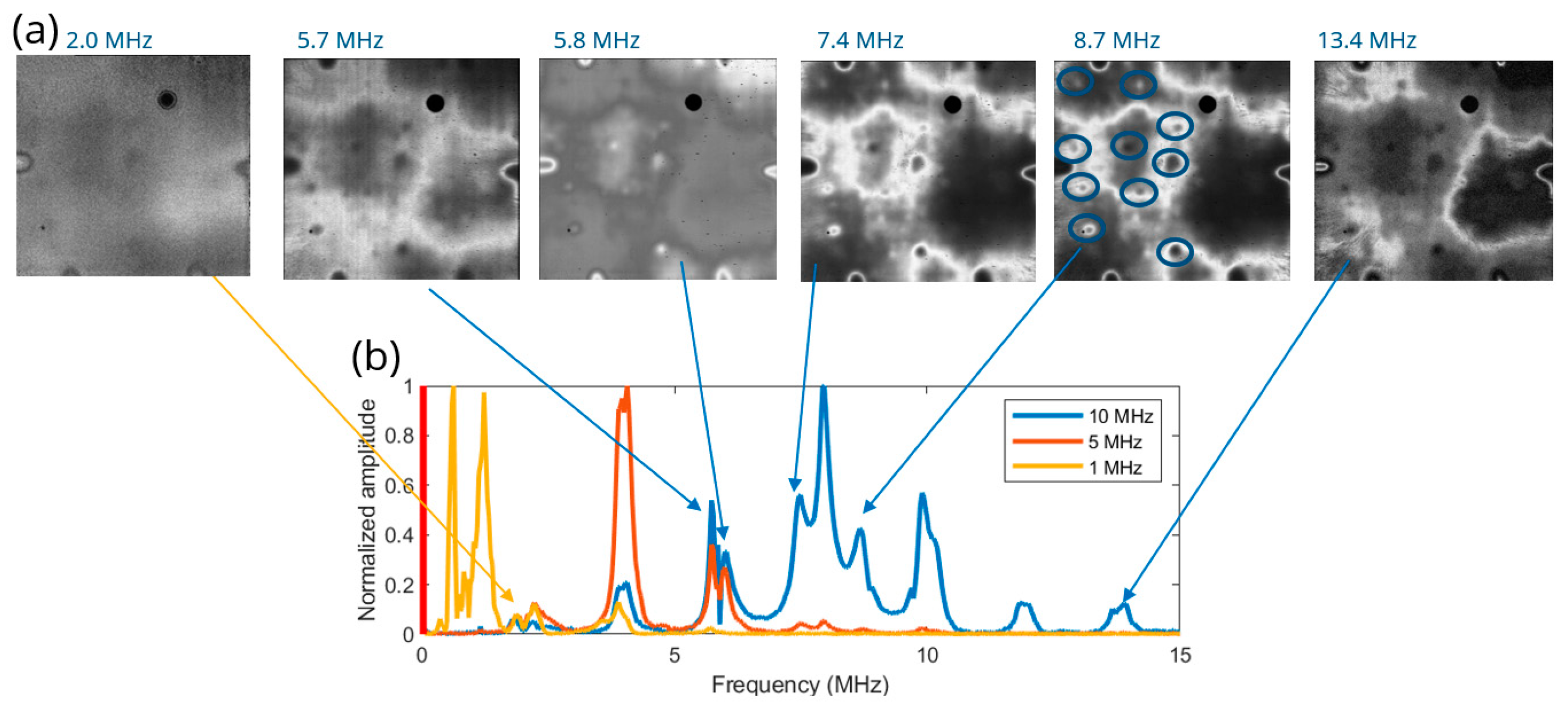
Figure 7 shows the normalized amplitude images at specific shoulder frequencies. These images are very different from the standard TT images, showing a lot more features. As with the insert panel case, lines that are bright can be traced on top of the surface, which can be attributed to a change in thickness. A similar pattern can be seen in the 3D scan of the KB panel. However, in these images, black or white spots are also present which cannot be attributed to changes in BL thickness and are also not present in the insert panel. When looking at the pattern of these spots, it more or less corresponds to the locations of the contaminants. By averaging the total amount of power over a specific frequency band, the white lines that are due to differences in BL thickness can be suppressed.

Figure 8 shows the result of averaging the frequency signal over a specific frequency range for the KB panel. The white bands in the images are not present anymore, but black and white spots can still be seen on the surface. The authors believe that it is these black spots than are an indication of the contaminants that were put on the surface (physical origin still unknown). In order to investigate this, tensile testing was carried out at the locations of these white and black spots.

3.4. Tensile Testing

Tensile testing was performed according to the TH14.5170-12E lap shear test. The samples were taken from subsections of the KB panel, as specified in Figure 9. In total, 11 samples were made, with 4 reference samples not containing any contamination indications in the frequency analysis and specified as KB-2-ref-xx. The other specimens cover a location that shows an contamination indication in the frequency analysis, either as a black spot or a white spot.

The results from the four reference samples are quite consistent, showing an mean load of 10.9 kN with a standard deviation of 0.08 kN. The maximum shear stress of the reference samples is 34.45 MPa with a standard deviation of 0.47 MPa. All reference samples have failed cohesively. Of the seven samples containing a contamination indication, only the KB-01 sample showed a reduction in adhesive strength. The other six had a mean maximum shear stress similar to the reference samples. All six of these samples failed cohesively. Sample KB-2-01 is the only one that showed a reduction in its maximum shear stress, with a total max load of 8.36 kN, resulting in a maximum shear stress of 26.15 MPa instead of 34.45 MPa, which is 75.9% of the maximum shear stress in the other samples. The failure mechanism is mixed-mode, with adhesive and cohesive failure seen. 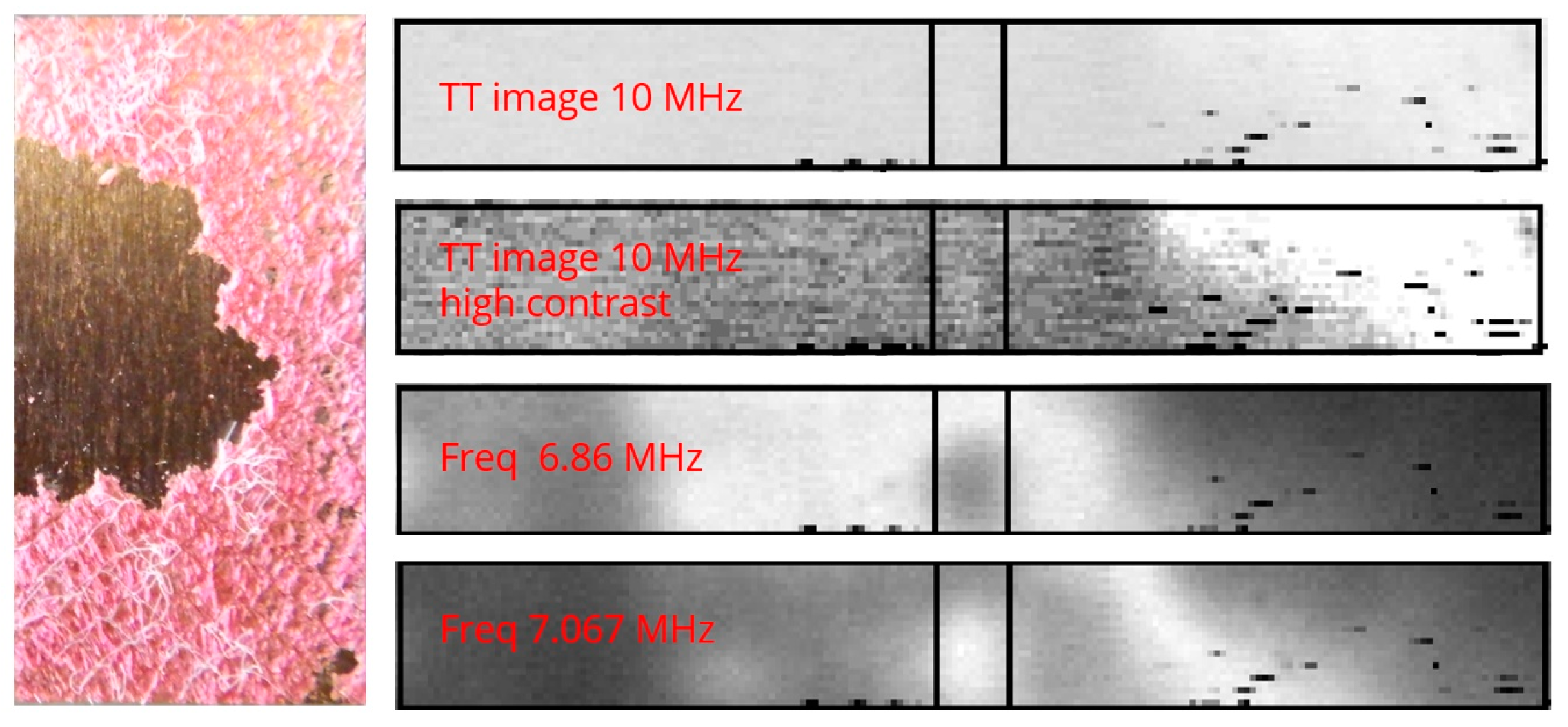Figure 10 shows a photograph of the failed interface and the corresponding C-scans of that location.

From the figure it can be seen that a part of the tested area failed adhesively, while the other part failed cohesively. From the “standard” TT C-scan results no indication of contamination is detected in the area that was tensile-tested. However, when performing the frequency analysis, a clear indication of contamination in the center of the tested interface can be detected, corresponding to the optical photograph of the tensile specimen. From the optical photograph, the area that has adhesively failed can be determined by image thresholding. This area corresponds to 27% of the total area. If this area is subtracted from the maximum shear stress calculations, the total strength would amount to 73% of a properly joined area. In testing, this amounted to 75.9%, indicating that the area that has failed contributed marginally to the total strength of the lap shear specimen. All other samples that also showed an indication of contamination in the frequency domain did not lead to a reduction in maximum shear stress.

4. Discussion

In this work, only two sheets of metal were bonded together, resulting in a single BL. It is shown that the adhesive’s thickness can be determined from the UT frequency data. However, real samples often contain multiple BLs and multiple stacks of sheets. It remains to be seen if the adhesive BL thicknesses can be extracted from multiple-BL panels.

The “kissing bond” panel shown in this work was produced multiple times. Results in the frequency domain are very consistent between the panels, meaning that each location that has been marked in the panel as a contamination indication also appears in the other panels, albeit at a slightly different location and size. Figure 11 shows this consistency in the amplitude data at 8.7 MHz.

For six of the seven tensile specimens no reduction in maximum shear stress was identified, while there were indications of contamination in the ultrasonic frequency analysis. The indications appeared as a change in amplitude with respect to the surrounding material. There are a number of ways in which this amplitude can vary, like differences in the speed of sound (due to different curing approaches), differences in adhesive thickness, and the presence of contaminants. Work is still ongoing in order to better classify when a change in amplitude can be considered a weak bond.

5. Conclusions

Normal TT C-scanning is able to detect all the inserts in the insert panel. However, there are differences in attenuation which can be contributed to the non-uniform thickness of the BL. By moving into the frequency domain, the shift in frequencies due to this change in thickness can clearly be seen. The frequency spectrum shows that the panel acts as a frequency filter, easily passing frequencies that are in resonance with the thickness of a single plate. The resonance frequencies also enable the measuring of the thickness of the BL. For the kissing bond panel, minor differences in the attenuation of the ultrasonic signal can be seen. The maximum of its TT signal suppresses a lot of information about the BL. By going into the frequency domain, the amplitude at the shoulders of the frequency peaks contains a lot more information. Bands that appear due to a thickness change in the BL can easily be detected, but bright and dark spots are also visible on these images. By taking the average of the frequency spectrum around a specific frequency, the banding due to a change in BL thickness can be suppressed, leaving only the bright and dark spots in the images as an indication that something is different. The pattern more or less matches the locations where the contaminations were placed. Single shear lap testing was performed on the locations that showed an indication of contamination in the frequency analysis. One of these locations showed a reduction in maximum shear stress, while the other indications had no reduction in shear stress. A weak bond was therefore successfully detected in the frequency analysis. However, the accuracy of this approach is still low, since it also identified six locations that had no reduction in maximum shear stress. More work needs to be carried out to improve the selectivity of this method.

References

- Guyott, C.C.H.; Cawley, P.; Adams, R.D. Use of the Fokker Bond tester on Joints with Varying Adhesive Thickess. Proc. Insitution Mech. Eng. Part B Manag. Eng. Manuf. 1987, 201, 41–49. [Google Scholar]
- Samaitis, V.S.; Yilmaz, B.; Jasiũniene, E. Adhesive bond quality classification using machine learning algorithms based on ultrasonic pulse-echo immersion data. J. Sound Vib. 2023, 546, 117457. [Google Scholar] [CrossRef]
- Jasiũniene, E.; Yilmaz, B.; Smagulova, D.; Bhat, G.A.; Cicénas, V.; Žukauskas, E.; Mažeika, L. Non-Destructive Evaluation of the Quality of Adhesive Joints Using Ultrasound, X-ray and Feature-Based Data Fusion. Appl. Sci. 2022, 12, 12930. [Google Scholar] [CrossRef]