On the Edge Model-Aided Machine Learning GNSS Interference Classification with Low-Cost COTS Hardware ^†

Abstract

Interference signals can disrupt global navigation satellite system (GNSS) receivers and degrade or deny a position-velocity-time (PVT) solution. After detecting an interference signal, classifying its type can provide insight into its cause and help determine the necessary next steps to counteract it. In this paper, we present a method for interference detection and a resource-efficient model-aided on-the-edge machine learning (ML) model for interference signal classification running on low-cost commercial-off-the-shelf (COTS) hardware, enabling a highly cost-effective spectral monitoring solution. The choice of detection metrics is justified based on real-world spectral monitoring data from a German highway and the capability of the ML model to generalize across different environments is demonstrated in an outdoor field test. Overall, we present an operationally ready GNSS interference detection and classification system.

1. Introduction

Interference signals can disrupt global navigation satellite system (GNSS) receivers [1]. The ability to classify the type of interference source helps counteract and eliminate an interference source after its detection. External electronic devices may generate harmonics that could explain a single-tone signal [2]; on the other hand, the illegal use of a privacy protection device (PPD) jammer may be the reason for receiving a chirp-type signal [3]. Some other signal types can indicate interference through legitimate spectral coexistence with different radio frequency systems [4,5,6]. Knowledge about the type of interference source gained through classification can give insight into the legitimacy and intent of the interference. This knowledge can then guide further steps towards its localization and, finally, its elimination.

Previously, van der Merwe et al. introduced a GNSS interference monitoring, detection, and classification system built around low-cost commercial-off-the-shelf (COTS) sensor hardware utilizing an external server for interference signal type classification [7]. This paper extends previous research by implementing an entirely local interference detection and classification on the low cost (LC) COTS sensor. We show that combining the previous detection strategy with an energy detector enhanced by noise floor compensation offers improved detection performance while reducing the need for manual calibration. Further, the proposed method exploits synergies between conventional statistical signal processing and machine learning (ML), allowing real-time interference signal classification without external processing. In addition, we present an end-user-oriented interface that enables non-expert users to operate the sensor intuitively. We conclude with an in-the-field sensor evaluation under real-world conditions, demonstrating its operational readiness with entirely local detection and classification capabilities.

2. Methods

2.1. Hardware Changes

The LC sensor comprises a Raspberry Pi 4B single board computer (SBC) (manufactured by the Raspberry Pi Foundation, Cambridge UK) for signal processing and system interfacing, a GNSS Raspberry Pi hat (pHat) for time synchronization and carrier-to-noise density ratio (CN0) monitoring, and an NeSDR SMArt v5 (manufactured by Nooelec, Wheatfield USA) as a software defined radio (SDR) radio-frequency front-end (RFFE). 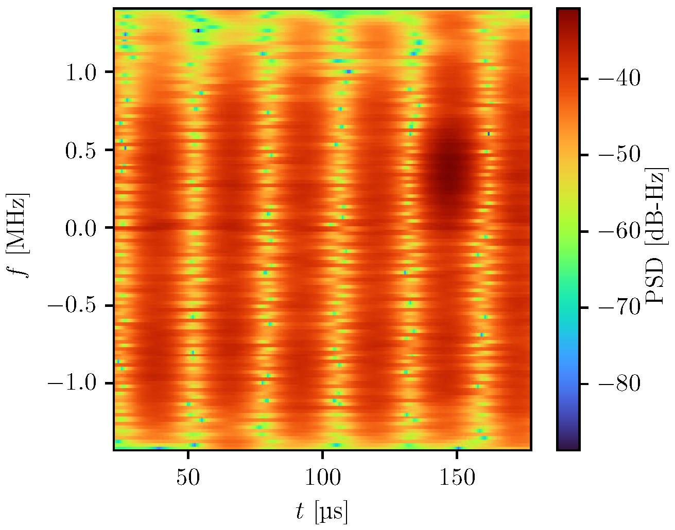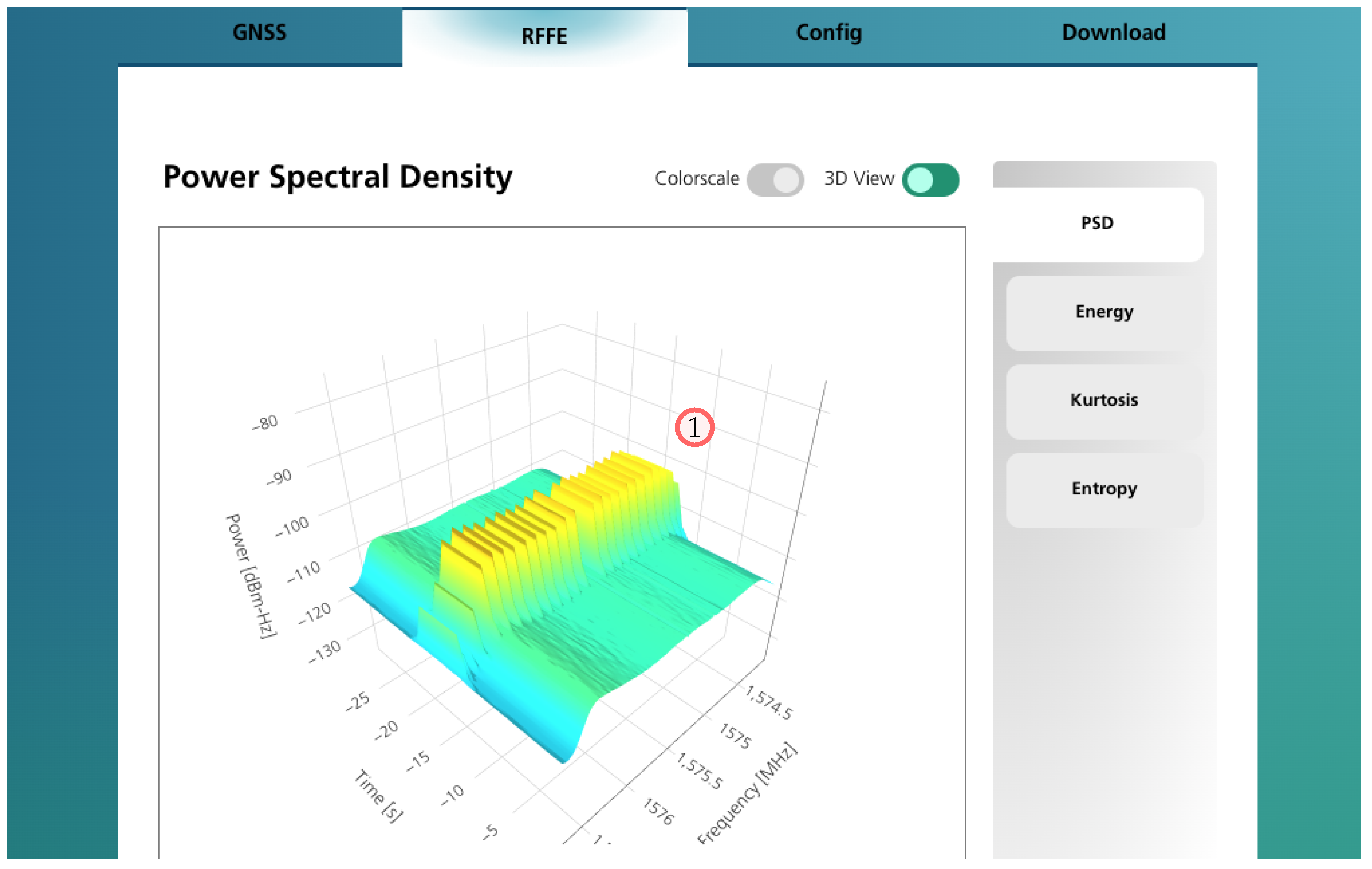We process the SDR samples in batches of $1\mathrm{s}$ to facilitate efficient processing. While detection and classification are possible in this configuration, a spectrogram with high time resolution, which might be of interest for manual identification of an interference source, can not be obtained. Therefore, a secondary NeSDR SMArt v5 works as a snapshot receiver. On trigger of the interference detection, the sensor stores a $20\mathrm{m}\mathrm{s}$ snapshot of unprocessed IQ samples, providing the maximum possible flexibility for subsequent analysis of a captured interference signal. 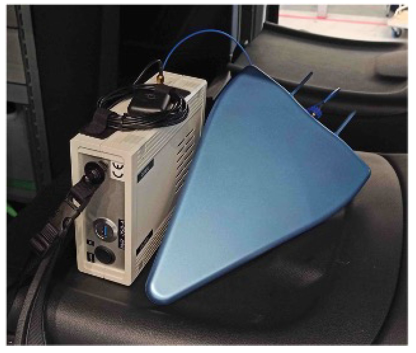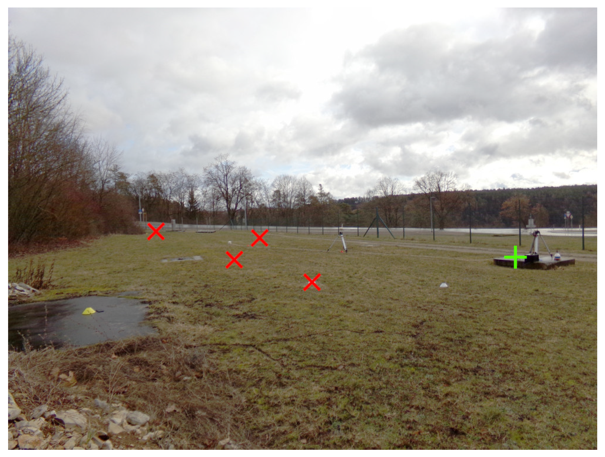An example spectrogram of a GNSS interference snapshot obtained with this SDR is shown in Figure 1. Three setups follow the described configuration: a battery-powered hand-held, a vehicle-mounted, and a stationary version optimized for long-term operation. The battery-powered hand-held version of the sensor is shown in Figure 2. Both SDRs have a sampling rate of $2.86\mathrm{MHz}$. Given the accumulation of samples for $1\mathrm{s}$, the computation for the features, the detection, and classification inferences are at a rate of $1\mathrm{Hz}$.

2.2. Interference Detection

Two popular approaches to interference detection previously discussed in the context of the LC COTS sensor are CN0 monitoring and a tuned energy detector [7]. Additionally, van der Merwe et al. explored in detail the usability of spectral entropy and spectral kurtosis for interference signal classification [6]. They show that these metrics can yield improved classification performance, even with limited bandwidth, such as the used SDR.

Given the input signal $x\left[k\right]$, the sampling time $T_s$ and an integration count M, the energy can be computed as [6]:

$$E=T_s\sum _{k=0}^{M-1}x\left[k\right]x^{*}\left[k\right]$$

(1)

For the spectral entropy, let $X_m\left[n\right]$ represent the n-th bin of the m-th short-time Fourier transform (STFT) of length N of $x\left[k\right]$. In addition, let K be the integration count, related to the integration count of the energy by $M=KN$. Then, the normalized spectral entropy with base 2 is computed as [6]

$$H_s=-{\displaystyle \frac{1}{{log}_{2}N}}\sum _{k=0}^{N-1}{s}_y\left[k\right]{log}_2{s}_y\left[k\right]$$

(2)

with the PSD normalized as a probability density function as [6]:

$$s_y\left[n\right]={\displaystyle \frac{{\displaystyle \sum _{k=0}^{K-1}}{\left|X_k\left[n\right]\right|}^2}{{\displaystyle \sum _{m=0}^{N-1}}{\displaystyle \sum _{k=0}^{K-1}}{\left|X_k\left[m\right]\right|}^2}}$$

(3)

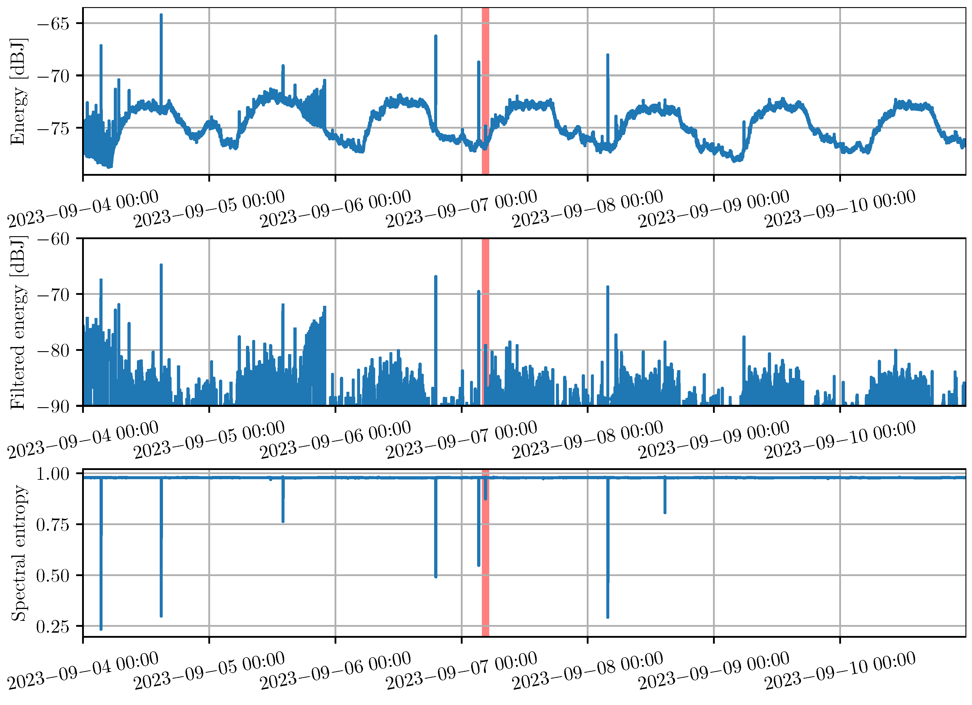
During the initial in-the-field evaluation of the LC sensor on German highways, we observed a daily oscillating pattern in the energy measurement—an example of this observation throughout one week is evident in Figure 3. This oscillatory behavior could, for instance, be due to daily fluctuations in traffic intensity and temperature. The energy measurement shows several large spikes that indicate the presence of an interfering signal. However, due to the large fluctuations as well as measurement noise, it is not apparent how to choose a fixed threshold for interference detection. The energy measurement shows peaks that correlate with a drop in entropy and, therefore, clearly indicate the presence of an interference signal. Yet the measured energy spike is vastly below the daily fluctuation level. One example is marked in Figure 3 by the shaded red area. While the energy peaks over the short-term noise floor during the interference event, it sits below the average long-term noise floor. Therefore, setting a fixed energy detection threshold will either yield many missed detections, as the threshold will need to sit above the maximum of the noise floor oscillation or lead to constant false positives when the noise floor rises beyond the threshold.

A second insight from Figure 3 is that the spectral entropy exhibits highly stable behavior, remaining nearly constant except for several sharp drops that mostly correlate with measured energy increases. A fixed threshold can easily detect these drops in spectral entropy. It is visible that not every strong entropy drop has a correspondingly large energy peak and vice versa. Van der Merwe et al. exploit this phenomenon to enable classification and discuss the sensitivity of the metrics to different interference signal types [6].

Accordingly, detection can be implemented as a mixed-decision process based on the spectral entropy $H_s$ and noise floor-compensated energy $\dot{E}$. By compensating for the noise floor’s long-term oscillation, setting a fixed threshold on the energy measurement becomes feasible again. The noise floor estimation is equivalent to a long-term exponentially weighted moving average over the linearized energy. We calculate the filtered energy by subtracting the noise floor estimate from the linearized energy. After compensating for unity gain at high frequencies, this is equivalent to applying a high-pass filter with the transfer function

$$G\left(z\right)={\displaystyle \frac{(1+\alpha )(1-z^{-1})}{2(1-\alpha z^{-1})}}$$

(4)

to the linearized energy E, where $\alpha$ determines the cut-off frequency. Empirically, an $\alpha =0.998$ value compensates correctly for the oscillatory behavior observed in Figure 1. Fundamentally, this approach assumes that interference signals appear and disappear quickly. An interference signal rising slowly in power would not be detected. Similarly, suppose an interfering signal is present for a long duration. In that case, the compensation mechanism will eventually compensate for its presence and not detect it after an initial correct detection. The sensor is intended to operate in a highway scenario, where interference sources, such as PPD jammers, are likely inside moving vehicles and therefore appear and disappear quickly. Therefore, this mechanism is suitable for the intended application.

As is visible in Figure 3, setting a threshold sufficiently low for triggering on the event marked by the red area in Figure 3 will lead to a significant number of triggers. For example, a noise-like rise in filtered energy is visible towards the end of 5 September 2023 or the beginning of the time series. However, upon close inspection of those areas in the dataset, periodic spikes in the measured energy are indeed present during those times. Therefore, several triggers of those events are, in fact, expected behavior. Given the normalized spectral entropy measurement $H_s$, a filtered energy measurement $\dot{E}$, the null-hypothesis ${\mathcal{H}}_0$ meaning “no interference is present”, and the alternate hypothesis ${\mathcal{H}}_1$ meaning “an interference is present”, the following decision rule is applied:

$$\begin{array}{c}\hfill \begin{array}{cc}\hfill H_s<{\gamma }_{H_s}\vee \dot{E}>{\gamma }_{\dot{E}}& :{\mathcal{H}}_1\hfill \\ \hfill H_s\ge {\gamma }_{H_s}\wedge \dot{E}\le {\gamma }_{\dot{E}}& :{\mathcal{H}}_0\hfill \end{array}\end{array}$$

(5)

The respective thresholds ${\gamma }_{H_s}$ and ${\gamma }_{\dot{E}}$ can be determined empirically for this set of features. They were obtained via grid search optimization of the $F_1$-score in the training dataset from the indoor testing hall that will be introduced in the classification section. Over the full training set, the mixed-decision detector with $F_1$-optimal thresholds achieves a precision of 89.9% and a recall of 83.0%, thus yielding $F_1\approx 0.863$. The thresholds resulting from the optimization are ${\gamma }_{\dot{E}}\approx -110.3\mathrm{d}\mathrm{BJ}$ and ${\gamma }_{H_s}\approx 0.992$. It should be noted that the value for ${\gamma }_{\dot{E}}$ is normalized to a reference level different from the one displayed in Figure 3. A common reference level can be established between the sensors through calibration.

2.3. Interference Classification

The typical approach for interference classification uses the STFT to create a spectrogram, where convolutional neural networks (CNNs) treat the spectrograms as images to classify the interference [8,9,10]. This approach attempts to exploit CNNs’ spatial invariance for generalization. However, the resulting network tends to be complex and extensive to achieve accurate classification. An alternate proposal involves using well-studied signal processing approaches combined with ML for a simpler processing pipeline while maintaining accurate classification [11]. Van der Merwe et al. designed an inference system that synergizes statistical signal processing with ML [6].

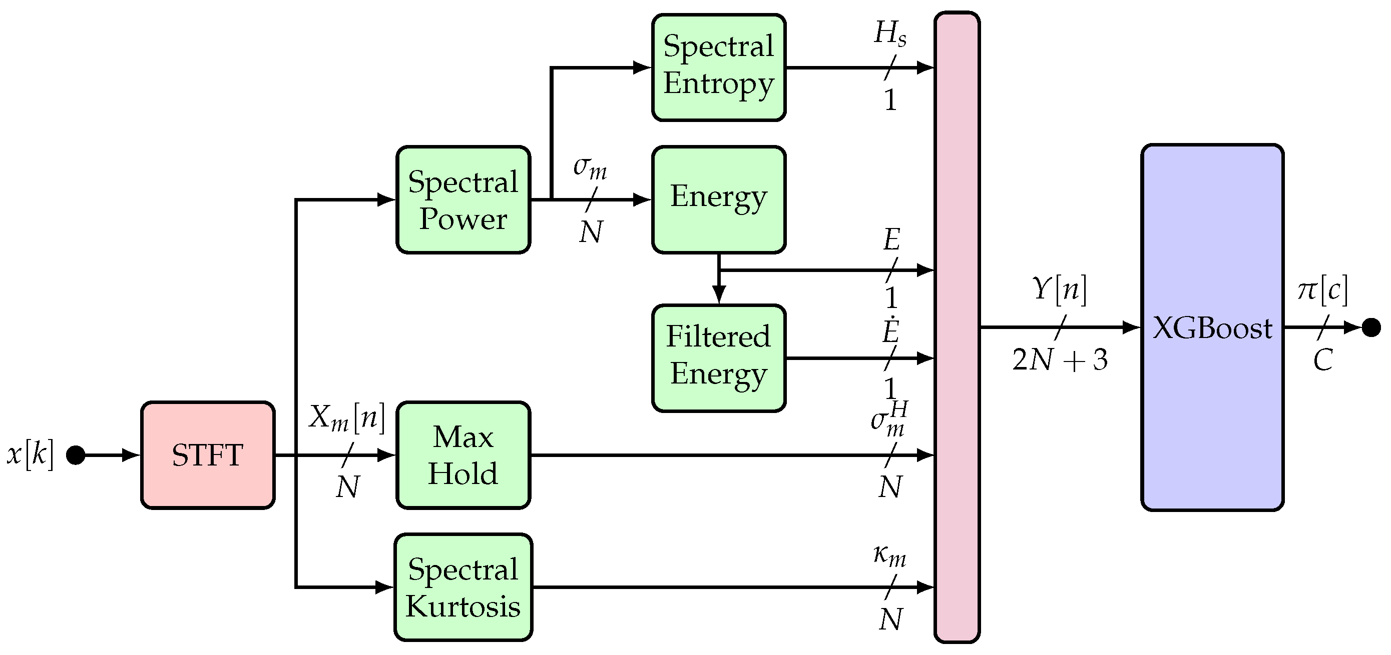
The processing model calculates the STFT to derive the spectral entropy and spectral kurtosis; the defined implementation calculates the STFT over 128 frequency bins. We also used the novel filtered energy metric as an additional statistical feature. Remember that for efficient processing, the system processes the samples to calculate the features in batches of 1 s; for the spectrum, a max-hold function keeps the highest value per channel for each batch; this is usually useful for short-lived signals when doing spectral monitoring. It then utilizes these spectral statistical features as input for the ML process. We selected extreme gradient boosting (XGBoost) as the underlying model because it has demonstrated remarkable performance in interference classification tasks and is an excellent classifier and regressor for tabular data [6,12,13]. Figure 4 gives a general overview of the classification pipeline.

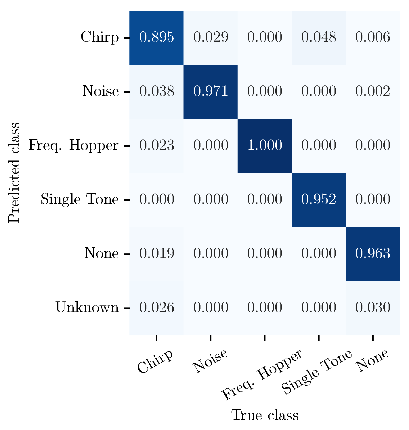
The model gives a probability distribution over the possible interference classes, including “None”, which means there is no interference. We observed a specific behavior on initial system tests when the system faced previously unseen signals: indecision between two classes, jumping between them in each sample, i.e., on each inference. To overcome this class uncertainty, the nearest neighbor distance ratio (NNDR) further restricts the inference; if the NNDR is below an empirically defined threshold, the system labels the class as “Unknown”. This certainty test restricts the system from classifying a signal only when there is absolute certainty and classifying the signal as unknown when there is not enough certainty on a specific class [14].

2.4. Learning Considerations

It is well known that a robust data-driven solution relies on a rich and representative dataset. For training, we set up a single LC sensor with an AAR HL 7040 antenna for high directionality inside the “Test and Application Center LINK” of Fraunhofer IIS in Nuremberg [15]; a signal generator played a variety of signals with a slow power sweep of −20 to 20 dBm lasting $1\mathrm{h}$ each sweep, changing the relative location of the signal generator to the sensor. To represent a variety of cases, the signal types used were single complex tone, linear chirp, parabolic chirp, frequency hoppper, and band-limited noise.

Lastly, the biggest challenge in this type of system lies in the sensor variability problem; this means that a model learns quite well the specific sensor on which the training data are recorded but fails to extrapolate or generalize the inference to other sensors; this is due to particular hardware imperfections to which ML models overfit. The solution is to use a class of domain adaptation [16,17,18]. The adaption we used extends the training dataset with “null” data from the target sensor. The model is thus trained on interference signals recorded on one sensor and from long-term recordings of multiple sensors with a 50-ohm resistor connected to the RFFE instead of an antenna. The recordings of the sensors with the resistor will only have information on the RFFE without any received signal; as such, the expectation is that the model can learn how the interference signals look given the features and how multiple RFFE front ends look without them. We call this learning process “null learning”. To test the capabilities of these generalizations, we perform real-world tests on sensors that never recorded interference signals but only “null” data and on various signals with configurations slightly different to those used during recording, e.g., chirp rate or single-tone center frequency.

2.5. End-User Optimization

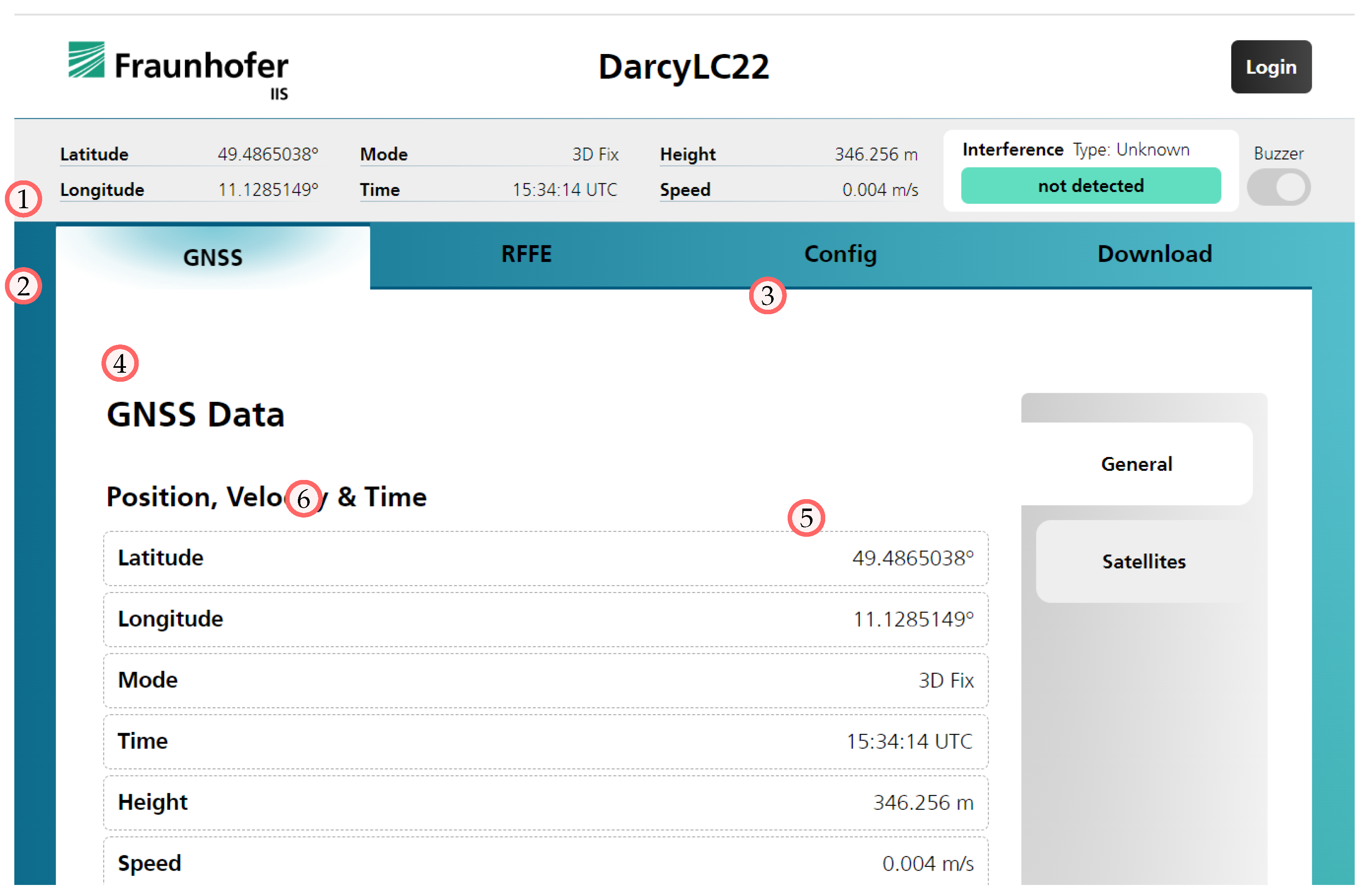
The general goal of the user interface is to simplify the interaction with the sensor. It should provide an intuitive operation without requiring a user with significant expertise. The general functional requirements were to visualize the spectral features and GNSS performance indicators clearly and offer a convenient and well-documented way to configure the sensor and download recorded features and raw snapshots as files. The end-user needs to see whether the system detected an interference quickly. As there is also a hand-held version of the sensor, it is also essential to use the interface on mobile devices such as a tablet or smartphone, i.e., responsive user interface design. Furthermore, there were less specific quality characteristics like reliability, performance, and basic security to consider.

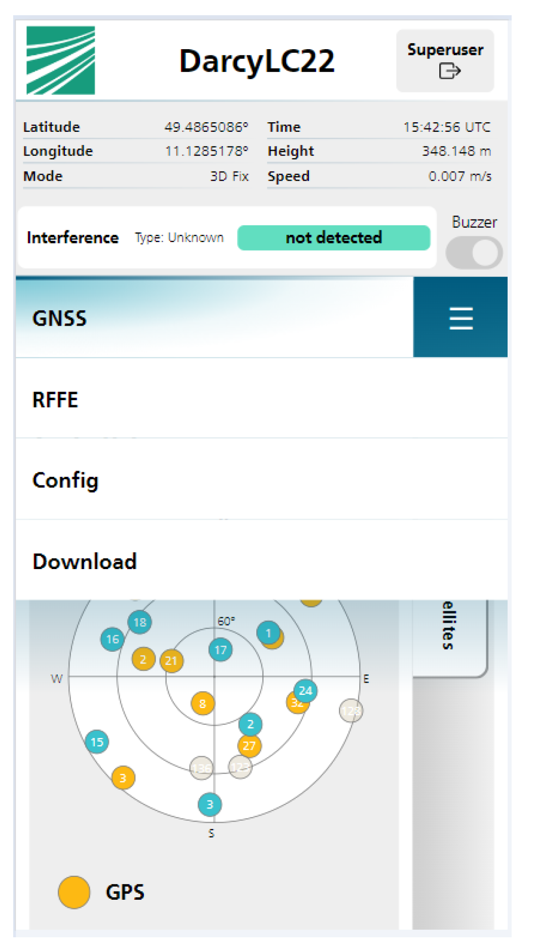
The final client application is a single-page web application (spa) running in the user’s device’s local browser. The sensor runs a web server to deliver the static spa files and the current sensor data to display in the application. Figure 5 shows the overall structure of the user interface. The header is a fixed component and displays data that need to be quickly visible. The interference detection and classification indicator (3) turns red and shows the classification result when an interference is detected. The central part of the spa is structured into four different pages (4), each further divided into subpages (5), to provide a clear overview of the available data and functionality the end-user can utilize. The user interface displayed on a mobile device such as a smartphone is shown in Figure 6.

The RFFE page contains the visualizations of the spectral features as can be seen in Figure 7. The Config page includes several sensor configuration forms. Every form provides a description and input validation of the single configurable parameters, as well as user feedback for the operation’s success. The whole application’s layout is responsive to the device’s screen size and, therefore, eligible for large-format Desktop screens as well as smartphones (see Figure 6).

3. Results

We validated all the sensor systems under realistic conditions with an outdoor field test. Since all training data of the ML model consist of recordings from an indoor testing hall and the “null” data, this test is a crucial indication of the ability of the model to generalize across different propagation environments. The test was hosted by German authorities and carried out in a restricted area where it could be conducted legally. The usage of the testing area put certain time constraints on the field test. Therefore, the test consisted of limited samples for each interference signal class. While this raises the uncertainty in the observed performance for some classes, the results still represent the achievable performance with the proposed methods.

Figure 8 shows the test setup. The distance between the jammer and the sensor antenna was approximately $10\mathrm{m}$. Using a COTS chirp jammer, additional tests were performed with a variation in the distance between 10 and $50\mathrm{m}$. Ranges beyond $50\mathrm{m}$ were not tested due to the space restrictions of the testing area. Additionally, an effective radius of 50 m is sufficient for the sensor’s initially intended application for spectral monitoring on highways.

The sensor produces feature sets and detection and classification results at $1\mathrm{Hz}$. The ground truth corresponding to the data was obtained by hand-labeling based on correlating the sensor data timestamps with the known timestamps of interference signal generation. In cases where the recorded data clearly indicate an offset of one or two seconds between the recorded timestamps of the interference and the interference actually being visible in the data, the boundaries were manually corrected to account for delays and errors in the manual recording of the timestamps.

Table 1. Sample counts of all classes in the dataset. “None” corresponds to no interference.

Chirp	Noise	Freq. Hopper	Single Tone	None
266	34	25	21	1790

shows the number of samples for each class in the dataset. The mixed-decision detector achieves a precision of 91.7%, a recall of 98.8%, and an $F_1\approx 0.951$ over these data, using the detection thresholds obtained through numerical optimization on the indoor training set. Figure 9 shows the classification performance.

In addition to evaluating 34 noise samples with a bandwidth of $2\mathrm{MHz}$, we also recorded 35 samples of a different noise signal with a bandwidth of $20\mathrm{MHz}$. Those additional samples were manually excluded from the evaluation because only the former noise signal was present in the training set. Including the wide-band noise samples would lead to a decreased correct classification percentage of approximately 63.8%, with most misclassifications attributed to the chirp class. Later tests show correct classification and generalization of a previously unseen, i.e., not part of the training data, COTS PPD chirp jammer. Characterizing the extent to which the model can generalize the learned classes remains an open question for future investigation.

4. Conclusions

We demonstrated a deployment-ready, low-cost COTS GNSS interference detection and classification sensor utilizing resource-efficient, on-the-edge model-aided machine learning. Filtered energy and spectral entropy were proposed as detection features that overcome the non-idealities of plain energy measurements in a real-world application. Outdoor field tests show the sensor’s operational readiness and the ML’s generalization ability across different environments. Examining the ML’s ability to generalize within the learned classes as well as integration of the CN0 into the current pipeline are interesting areas of future study.

References

1. Dovis, F. (Ed.) GNSS Interference, Threats, and Countermeasures; Artech House GNSS Technology and Applications Series; Artech House: Boston, MA, USA, 2015. [Google Scholar]
2. Hegarty, C.J.; Bobyn, D.; Grabowski, J.; Van Dierendonck, A. An overview of the effects of out-of-band interference on GNSS receivers. Navigation 2020, 67, 143–161. [Google Scholar] [CrossRef]
3. Van Der Merwe, J.R.; Rugamer, A.; Garzia, F.; Felber, W.; Wendel, J. Evaluation of mitigation methods against COTS PPDs. In Proceedings of the 2018 IEEE/ION Position, Location and Navigation Symposium (PLANS), Monterey, CA, USA, 23–26 April 2018; pp. 920–930. [Google Scholar] [CrossRef]
4. Xingxin Gao, G. DME/TACAN interference and its mitigation in L5/E5 bands. In Proceedings of the 20th International Technical Meeting of the Satellite Division of the Institute of Navigation 2007 ION GNSS 2007, Fort Worth, TX, USA, 25–28 September 2007. [Google Scholar]
5. Schütz, A.; Kraus, T.; Lichtenberger, C.A.; Pany, T. A Case Study for Potential Implications on the Reception of Galileo E6 by Amateur Radio Interference on German Highways Considering Various Transmitter-receiver-signal Combinations. In Proceedings of the 34th International Technical Meeting of the Satellite Division of The Institute of Navigation (ION GNSS+ 2021), St. Louis, MO, USA, 20–24 September 2021; pp. 1687–1696. [Google Scholar] [CrossRef]
6. Van Der Merwe, J.R.; Franco, D.C.; Feigl, T.; Rügamer, A. Optimal machine learning and signal processing synergies for low-resource GNSS interference classification. IEEE Trans. Aerosp. Electron. Syst. 2024, 60, 2705–2721. [Google Scholar] [CrossRef]
7. Van Der Merwe, J.R.; Contreras Franco, D.; Hansen, J.; Brieger, T.; Feigl, T.; Ott, F.; Jdidi, D.; Rügamer, A.; Felber, W. Low-Cost COTS GNSS Interference Monitoring, Detection, and Classification System. Sensors 2023, 23, 3452. [Google Scholar] [CrossRef] [PubMed]
8. Brieger, T.; Raichur, N.L.; Jdidi, D.; Ott, F.; Feigl, T.; van der Merwe, J.R.; Rügamer, A.; Felber, W. Multimodal Learning for Reliable Interference Classification in GNSS Signals. In Proceedings of the 35th International Technical Meeting of the Satellite Division of the Institute of Navigation (ION GNSS+ 2022), Denver, CO, USA, 19–23 September 2022. [Google Scholar] [CrossRef]
9. Morales Ferre, R.; de la Fuente, A.; Lohan, E.S. Jammer Classification in GNSS Bands Via Machine Learning Algorithms. Sensors 2019, 19, 4841. [Google Scholar] [CrossRef] [PubMed]
10. Mehr, I.A.E.; Dovis, F. A Deep Neural Network Approach for Detection and Classification of GNSS Interference and Jammer. TechRxiv 2023. [Google Scholar] [CrossRef]
11. Dahrouj, H.; Alghamdi, R.; Alwazani, H.; Bahanshal, S.; Ahmad, A.A.; Faisal, A.; Shalabi, R.; Alhadrami, R.; Subasi, A.; Al-Nory, M.T.; et al. An Overview of Machine Learning-Based Techniques for Solving Optimization Problems in Communications and Signal Processing. IEEE Access 2021, 9, 74908–74938. [Google Scholar] [CrossRef]
12. Grinsztajn, L.; Oyallon, E.; Varoquaux, G. Why do tree-based models still outperform deep learning on typical tabular data? In Proceedings of the Thirty-Sixth Conference on Neural Information Processing Systems Datasets and Benchmarks Track, Virtual, 28 November 2022. [Google Scholar]
13. Shwartz-Ziv, R.; Armon, A. Tabular data: Deep learning is not all you need. Inf. Fusion 2022, 81, 84–90. [Google Scholar] [CrossRef]
14. Mendes Júnior, P.R.; de Souza, R.M.; Werneck, R.d.O.; Stein, B.V.; Pazinato, D.V.; de Almeida, W.R.; Penatti, O.A.B.; Torres, R.d.S.; Rocha, A. Nearest neighbors distance ratio open-set classifier. Mach. Learn. 2017, 106, 359–386. [Google Scholar] [CrossRef]
15. Aaronia, A.G. Logper Antennas Hyperlog 70 Series; Aaronia, A.G.: Strickscheid, Germany, 2023. [Google Scholar]
16. Han, Z.; Sun, H.; Yin, Y. Learning Transferable Parameters for Unsupervised Domain Adaptation. IEEE Trans. Image Process. 2022, 31, 6424–6439. [Google Scholar] [CrossRef] [PubMed]
17. Hussein, A.; Hajj, H. Domain Adaptation with Representation Learning and Nonlinear Relation for Time Series. ACM Trans. Internet Things 2022, 3, 1–26. [Google Scholar] [CrossRef]
18. Zhao, A.; Ding, M.; Lu, Z.; Xiang, T.; Niu, Y.; Guan, J.; Wen, J.R. Domain-Adaptive Few-Shot Learning. In Proceedings of the 2021 IEEE Winter Conference on Applications of Computer Vision (WACV), Waikoloa, HI, USA, 3–8 January 2021; pp. 1389–1398. [Google Scholar] [CrossRef]
Figure 1. Short excerpt of a spectrogram generated from a raw IQ snapshot from the LC sensor. The presence of an interfering chirp signal is visible. Due to the limited sampling rate of the SDR, the waveform appears similar to that of a pulsed signal. The power spectral density (PSD) is not normalized to a fixed reference level.
Engproc 88 00051 g001
Figure 2. The battery-powered hand-held sensor (left) connected to a directional antenna (right). The user carries the sensor with a carrying strap and can access the user interface via a smartphone or tablet which connects to the sensor’s WiFi access point.
Engproc 88 00051 g002
Figure 3. Energy and spectral entropy in part of the E1 band and filtered energy as recorded by the LC sensor over one week at a German highway during the initial in-the-field evaluation of the sensor. The energy and filtered energy are not normalized to a fixed energy reference level. The red bar highlights an interference event that is difficult to detect using a fixed threshold on the unfiltered energy.
Engproc 88 00051 g003
Figure 4. Feature processing and classification pipeline. N stands for the number of frequency bins processed with the STFT. At the end of the pipeline, the model outputs a probability π for each of the defined C number of classes.
Engproc 88 00051 g004
Figure 5. The user interface on a normal-sized notebook screen. (1) first header bar with logo, name, login and info button, (2) Current PVT data, (3) interference detection and classification indicator, (4) tabs, (5) tabs for the subpages, (6) content of the subpage “General” of the GNSS page.
Engproc 88 00051 g005
Figure 6. Mobile view of the user interface with extended burger menu.
Engproc 88 00051 g006
Figure 7. The “RFFE” page with the PSD plot. (1) a peak in the plot indicating a temporarily occurring jammer.
Engproc 88 00051 g007
Figure 8. Layout of the field test. The tested jammer positions are marked with an “x”, the sensor antenna position is marked with a “+”.
Engproc 88 00051 g008
Figure 9. Confusion matrix for the classification during the field test.
Engproc 88 00051 g009